
Quantifying Changes of Villages in the Urbanizing Beijing Metropolitan Region: Integrating Remote Sensing and GIS Analysis


1
State Key Laboratory of Urban and Regional Ecology, Research Center for Eco-Environmental Sciences, Chinese Academy of Sciences, Beijing 100085, China
2
University of Chinese Academy of Sciences, Beijing 100049, China
3
Chinese Academy for Environmental Planning, Beijing 100012, China
4
Beijing Institute of Surveying and Mapping, Beijing 100038, China
*
Author to whom correspondence should be addressed.
Remote Sens. 2017, 9(5), 448; https://doi.org/10.3390/rs9050448
Submission received: 15 March 2017
/
Revised: 16 April 2017
/
Accepted: 3 May 2017
/
Published: 6 May 2017
(This article belongs to the Special Issue Remote Sensing of Urban Ecology)
Abstract
:Rapid urbanization has resulted in great changes in rural landscapes globally. Using remote sensing data to quantify the distribution of rural settlements and their changes has received increasing attention in the past three decades, but remains a challenge. Previous studies mostly focused on the residential changes within a grid or administrative boundary, but not at the individual village level. This paper presents a new change detection approach for rural residential settlements, which can identify different types of rural settlement changes at the individual village level by integrating remote sensing and Geographic Information System (GIS) analyses. Using multi-temporal Landsat TM image data, this approach classifies villages into five types: “no change”, “totally lost”, “shrinking”, “expanding”, and “merged”, in contrast to the commonly used “increase” and “decrease”. This approach was tested in the Beijing metropolitan area from 1984 to 2010. Additionally, the drivers of such changes were investigated using multinomial logistic regression models. The results revealed that: (1) 36% of the villages were lost, but the total area of developed lands in existing villages increased by 34%; (2) Changes were dominated by the type of ‘expansion’ in 1984–1990 (accounted for 43.42%) and 1990–2000 (56.21%). However, from 2000 to 2010, 49.73% of the villages remained unchanged; (3) Both topographical factors and distance factors had significant effects on whether the villages changed or not, but their impacts changed through time. The topographical driving factors showed decreasing effects on the loss of rural settlements, while distance factors had increasing impacts on settlement expansion and merging. This approach provides a useful tool for better understanding the changes in rural residential settlements and their associations with urbanization.

1. Introduction
Rapid urbanization has led to great changes in rural landscapes [1,2,3]. During the process of urbanization, many villages grow into towns and cities, or become part of a city due to urban expansion [4,5]. In addition, rural households far from the city are increasingly moving into cities and finding seasonal or permanent employment, and sending remittances back to the villages [6]. This increased connectivity between urban and rural areas may also lead to great changes in rural villages [6,7]. These changes have marked ecological and environmental impacts, such as the loss of habitat and increased habitat fragmentation, loss of biodiversity, farmland loss and fragmentation, and urban heat islands [8,9,10,11,12,13]. Understanding how rural villages have changed over time and the drivers of change is crucially important for quantification of ecological and environmental impacts.
Remote sensing has been widely used for change analysis on rural landscapes, or more specifically, rural residential settlements (i.e., the artificial lands in rural areas), with the advantages of explicitly and periodically providing their spatial pattern over a large geographic area [14,15,16,17]. These studies may be loosely classified into two categories based on their analytical unit: grid-based and administrative boundary-based. The former uses a grid with a certain size as the unit of analysis to quantify the proportional cover of rural residential settlements and their changes [18,19,20,21]. For example, Tian et al. [19] used a grid of one kilometer and land use/land cover (LULC) maps derived from 30 m Landsat TM imagery to quantify changes in rural residential settlements and differences among 33 rural landscapes in China during the 1990s. A vegetation index, such as the Enhanced Vegetation Index (EVI) from the MOD13Q1 product, was also used to estimate impervious surfaces and their change in rural areas [17]. Another frequently used approach in previous studies was to quantify the proportional cover of rural residential settlements and their changes within the administrative units, ranging from county to prefecture city, and even to the national scale [22,23,24]. For example, Long et al. [21] investigated five regions of the Yangtze River watershed from the lower to the upper reaches using an administrative unit approach and found different phases of transitions in rural settlement land.
Previous studies only identified the increase or decrease of rural settlements at the administrative or grid level [4,17,25]. However, few studies have examined the changes at the village scale; that is, using the individual rural settlements as the unit of analysis. In fact, such information is crucially important for understanding the fate of each individual rural settlement, but is not available from the abovementioned analyses or methods. For example, how many villages (or what proportion of villages) were totally lost, expanded, or shrunken during the process of urbanization? Or, are villages close to the city (i.e., in the peri-urban areas) more likely to become part of the city or expand to become another town or city?
Here, we present a new approach to identify different types of changes at the individual rural settlement level by integrating remote sensing and GIS analyses. We further applied this approach to quantify the spatiotemporal patterns of rural residential settlements in the Beijing metropolitan area from 1984 to 2010. Additionally, we investigated the drivers of such changes. Specifically, we addressed two research questions: (1) What are the spatiotemporal patterns of rural residential settlement change in the Beijing metropolitan area? (2) what are the driving forces of rural residential settlement change, their relative importance, and their temporal dynamics? We used Landsat TM data collected in 1984, 1990, 2000, and 2010, in combination with other GIS layers for the analysis of settlement dynamics. We used multinomial logistic regression models to examine the effects of the driving forces on changes.
2. Materials and Methods
2.1. Study Area
Beijing is the capital of China, located in the North China Plain, between 39°28′–41°25′N and 115°25′–117°30′E (Figure 1). It has a total area of approximately 16,410 km2. The western and northern parts of Beijing are mountainous and the other parts are plains with very high density of rural residential lands [19]. Since the implementation of the Reform and Opening policy, Beijing has been experiencing rapid urbanization, associated with unprecedented land use/land cover changes: the proportion of urban population in Beijing increased from 54.96 to 86.42% during 1978–2014, and the developed land area increased from 1536 km2 to 3075 km2. By 2014, Beijing contained 3937 villages, with a total rural permanent resident population of 2.93 million [26].
With rapid urbanization, rural residential settlements in Beijing have also experienced dramatic changes since the 1980s. In Fengtai district, for example, the total area of rural residential settlements increased by 949.8 hm2 during 1984–1999, from 2059.7 hm2 to 3009.5 hm2, and its proportion increased from 6.87% to 10.03% [27]. In Beijing, there are four types of functional zones with different functional orientation and policy. The Capital Function Area (CFA) includes Dongcheng and Xicheng districts; the Urban Function Expansion Area (UFEA) includes the districts of Chaoyang, Haidian, Fengtai and Shijingshan; the Urban Development Area (UDA) includes the districts of Changping, Shunyi, Tongzhou, Daxing, and Fangshan; and the Ecological Conservation Zones (ECZ) includes the districts of Huairou and Pinggu, and counties of Yanqing and Miyun. At present, the administrative hierarchy of a city in China has three main administrative levels: City-County (district)-Township. Accordingly, the built-up area is usually classified into City Built-up Area (CiBA) and County Built-up Area (CoBA), which are the political-economic centers in the city and county, respectively.
2.2. Data Sources
Data used in this study included Landsat TM imagery, digital elevation models (DEM) and transportation maps. Landsat TM imagery of 1984, 1990, 2000, and 2010 was acquired from the United States Geological Survey (USGS), which has been widely used to investigate spatial changes of human settlements [19,28]. We acquired the SRTMDEMUTM 90-m resolution DEM products from the Computer Network Information Center, Chinese Academy of Sciences (http://www.gscloud.cn), which were used to measure the elevation and slope of rural settlements. The transportation maps were from Baidu Map™, which included a point layer that had the center positions of cities, counties, towns and villages (i.e., rural settlements), and a layer of linear features of roads. A vector layer of different levels of administrative boundaries was also used in this study.
2.3. Land Use/Land Cover Classification
An object-based backdating approach that integrates the backdating approach with an object-based method was used for Land Use/Land Cover (LULC) classifications, which included six classes; namely forest, grassland, farmland, water, artificial area (i.e., developed land), and bare land [16]. With this approach, the LULC maps from 1984 to 2010 were generated by the following three steps:
- (1)
- Creating the reference map: We first derived the 2010 LULC map from 2010 Landsat TM imagery by an object-based classification approach. The multi-resolution segmentation algorithm using a bottom-up region merging technique was used for the segmentation [29]. We created three levels of objects by setting different scale parameters; that is, 10 (level 1) for extracting water, grass and bare land; 30 (level 2) for extracting farmland and artificial land; and 50 (level 3) for identifying forest. A decision tree approach was used and the rulesets were created based on the spectral information, spatial relations and geometric characteristics. Extensive manual editing was conducted to further refine the classifications in order to obtain a highly accurate reference LULC map. We conducted accuracy assessment by selecting 300 random points using a stratified sampling method, with at least 30 samples for each category. We used 2.4 m QuickBird images and 2.5 m SPOT 5 images as reference data for accuracy assessment. The overall accuracy of the 2010 LULC map was 96% [16].
- (2)
- Creating LULC maps for other years: Using this 2010 LULC map as the reference map, the LULC classification maps in 2000, 1990, and 1984 were derived separately by an object-based backdating approach [16]. Taking the 2000 LULC map for example, we first used change vector analysis to identify the areas with changes from 2000 to 2010, which were then classified using the object-based classification method. For the areas with no change, the LULC type in 2010 was backdated to the map of 2000. More details about the classification approach can be found in Yu et al. [16]. Similarly, for the 1990 and 1984 LULC maps, we also used the 2010 LULC map as a reference map to reduce the error propagation.
- (3)
- Accuracy assessment: Accuracy assessment was also conducted for the LULC classification maps in 2000, 1990 and 1984, using the same procedure as that for the 2010 LULC. We used high spatial resolution satellite images and historical aerial photos as reference data for the years 2000 and 1990. The 1984 LULC classification was mostly evaluated based on visual interpretation of the Landsat TM data, because of the lack of historical aerial photos. The overall accuracies of these 3 classification maps were 86.11% in 1984, 85.87% in 1990, and 88.03% in 2000.
2.4. Change Analysis on Rural Residential Settlements
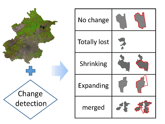
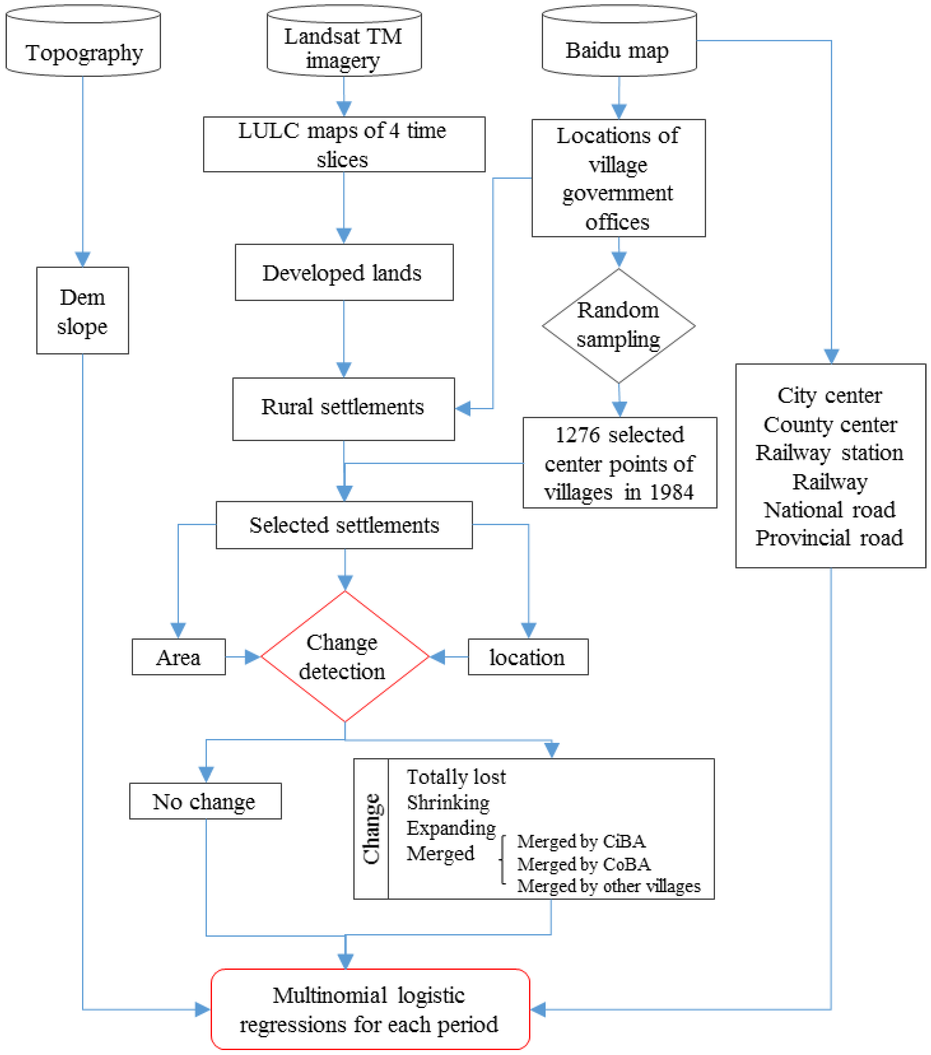
To detect the change of rural residential settlements, we first randomly selected a subset of rural residential settlements from the 1984 LULC map, based on the center points of village government offices in the database of Baidu Map. We then developed a new approach to detect the area changes of these settlements in 1984–1990, 1990–2000, and 2000–2010, respectively. This approach classified the changes of the residential settlements into 5 types: “no change”, “totally lost”, “shrinking”, “expanding”, and “merged”. Additionally, “merged” was further divided into 3 sub-classes: “merged by CiBA”, “merged by CoBA”, and “merged with other villages” (Figure 2).
2.4.1. Select Rural Residential Settlement Patches
Random sampling of the center points of villages: There were 4326 villages in Beijing in 1984, with much higher density in the plain region, but sparse in the mountain area. To reduce the effects of spatial autocorrelation of different explanatory variables and to maximize the number of samples, we selected a subset of the villages using a random sampling approach with a minimum threshold of 400 m for distance [30,31,32]. Consequently, we randomly selected 1276 center points of villages in 1984, based on the database of Baidu Map, historical Landsat images collected in 1984 and some ancillary historical maps, 30% of the total, and the average of the distances between neighboring villages was 1585 m.
Extracting the rural residential settlements: We focused on the changes in the rural residential settlement of the villages, which were defined in this research as spatially continuous artificial areas in the village, and where the local government office of a village was typically located in Beijing. Specifically, the rural residential settlements were identified and selected in three steps: (1) We selected the class objects “artificial area” from the LULC maps as potential rural residential settlements; (2) The rural residential settlements in each year (1984, 1990, 2000, and 2010) were separated from cities and towns using the vector layer of points of cities, towns, and villages; (3) A subset of the rural residential settlements in 1984 were identified and selected by the 1276 center points mentioned above, which were used in the further change analysis from 1984–1990, 1990–2000, and 2000–2010, respectively.
2.4.2. Classifying Change Types
Defining the change types of rural settlements: Rural residential settlements were classified into 2 classes—“change” or “no-change” (Example a in Table 1). Residential settlements with changes were further classified into 4 types: “totally lost”, “shrinking”, “expanding”, and “merged”. The class “totally lost” refers to the settlements that were totally transformed into the other LULC types (Example b). The class “shrinking” refers to the settlements that were partly removed and where the size of the patch became smaller (Example c). The class “expanding” refers to the settlements whose size became larger (Example d). The class “merged” means a settlement merged with other settlements, including 3 sub-types: “merged by CiBA”, “merged by CoBA”, and “merged with a town center or other village(s)” (Example e, f, and g in Table 1).
Detecting the change types of rural settlements: The first four change types were identified by examining the area changes of each rural residential settlement (i.e., patch or polygons) between two time slices. We set 3600 m2 (the size of 4 pixels of Landsat TM data) as the threshold for change, because typically only a land cover object larger than 4 pixels can be readily recognized from the remote sensing image [33,34]. By contrast, the “merged” type—the last but special type of “change”—was examined using both the spatial position and attribution information of each rural residential settlement. Taking the settlement change in 1984–1990 as an example, detecting the type of “merged” was carried out by following 4 steps: (1) We first assigned each rural residential settlement a unique identification (ID) number. We did this separately for the years 1984 and 1990; (2) We created a new point layer using the geographic center point of each settlement in 1984, and the same ID number of the settlement (polygon) was used for each point; (3) Each center point in 1984 was then appended to the polygon layer of the 1990 settlements based on spatial location. The case that more than two center points with different IDs in 1984 were located in one polygon (i.e., settlement) in 1990 indicated that these two initially separated rural settlements in 1984 were merged into one in 1990; (4) Finally, the class “merged” was further separated into 3 sub-types, based on the information of the merged settlement in 1990 (e.g., the name and administrative level), as described above.
2.5. Potential Driving Factors for Rural Settlement Change
We selected both topographical and distance variables as potential predictors (Table 2). These variables were selected based on previous studies [25,35]. Specifically, we chose two topographical variables, elevation and slope, which have been considered as the foundation for people to settle down since ancient agricultural times [1]. These two variables were calculated from the DEM products.
In addition, we selected six distance (or proximity) variables: (1) Distance to city center (D2CiC); (2) Distance to county center (D2CoC); (3) Distance to rail station (D2RaS); (4) Distance to railway (D2RaW); (5) Distance to national road (D2NaR); and (6) Distance to provincial road (D2PrR) (Table 2, Figure 3). Compared to the relatively constant topographical conditions, distance variables may have more important effects on landscape changes, especially in residential areas with intensive human activities [36,37]. These distance factors have been widely used in previous studies and significantly affect land use change [2,25,38,39,40,41]. These variables were calculated based on land cover/land use maps and road layers in 1984, 1990, 2000, and 2010, using Spatial Analyst in ArcGIS™ 10.2. We did not consider the population, income, investment, and policy in this study, because the resolution of these data was too coarse for our village-scale research [37,42,43].
2.6. Statistical Analysis
Logistic regression has been widely used in quantifying the effects of the driving factors on LULC change [30,39,44,45]. In order to deal with the multiple change types of rural residential settlement (i.e., the four types of change and no change) (Table 2), we selected multinomial logistic regression (MLR) to investigate the effects of several selected variables on the probability of different possible outcomes of changes for each time period. MLR generalizes logistic regression to multiclass problems, i.e., with more than two possible discrete outcomes [46].
Assume that we have possible outcomes with multinomial probabilities . The probabilities are parameterized as
and
The log-odds interpretation of the logistic regression model takes the following form:
where group 1 in this study is the type of settlement of “no change” that was used as the standard/reference category; P1 is the probability of settlement with “no change”, and pk is that of type K; ak is the intercept, βk is the partial regression coefficient. After variable standardization, a larger absolute value of βk indicated greater influence on . x are driving factors, and g is the total number of possible outcomes.
Percent Correct Predictions (PCP) and Nagelkerke’s R2 were used to evaluate the performance of the logistic regression models. These both indicate the performance of the model, with maximum values of 1, meaning perfect fit. It should be noted that PCP is more frequently used to evaluate the performance of the model, and that the R2 in multinomial logistic regression is usually much lower than that in linear regression [47]. The case of R2 > 0.2 indicates a relatively good fit [48].
3. Results
3.1. Spatiotemporal Patterns of Rural Residential Settlements
While the number of rural residential settlements decreased sharply, the total area greatly increased. The randomly selected 1276 rural settlements in 1984 decreased rapidly to 812 in 2010, a loss of 36% of the villages over thirty years (Table 3). A total of 221 villages were lost during 1984–1990, 129 in 2000–2010, and 114 in 1990–2000. In contrast, the total area of artificial land for existing rural residential settlements increased by 128 km2 during 1984–2010, an increase of 34% of artificial land. The largest increase of 85 km2 occurred during 2000–2010 (Table 3).
The number of rural residential settlements in different change types varied with time, and the main change type shifted from ‘expansion’ to ‘no change’ (Table 4). During 1984–1990 and 1990–2000, only 132 (or 10.3%) and 94 (or 8.91%) of the rural settlements remained unchanged. From 2000 to 2010, however, 468 of the sampled villages (or 49.7%) remained unchanged. In contrast, the number of settlements that were totally lost or shrunken continually decreased. In all the three time periods, great proportions of villages were expanding and fewer villages merged with other villages or cities.
Spatially, most of the rural residential settlements with changes were located in the plain, especially in the Urban Development Areas (UDA) (Figure 4). The total number of settlements in UDA were 859 in 1984–1990, 741 in 1990–2000, and 658 in 2000–2010, consisting of 67.32%, 70.24%, and 69.93% of all the sampled settlements in Beijing, respectively (Table 5). Additionally, settlements that expanded or were merged in UDA both increased with time. For example, the total numbers of expanding settlements in UDA were 358, 409, and 239 in each time period, accounting for 64.62%, 68.97%, and 73.54% of all the sample villages that experienced expansion in Beijing, respectively. Similarly, the total expanded areas of rural residential settlements in UDA were 82.72 km2, 82.83 km2, and 190.99 km2 in each time period, accounting for 53.79%, 58.51%, and 86.98% of the total area of expanded rural settlements, respectively (Table 6). In contrast, the number of total settlements in the Urban Function Expansion Area (UFEA) decreased continuously from 90 (or 7.05%) to 40 (or 4.25%). There was no settlement in the Capital Function Area (CFA) during the study period.
3.2. The Relative Importance of the Driving Forces in Different Time Periods
The multinomial logistic regression models explained the variance in changes of rural settlements well (Table 7). All these models were significant at the 0.01 level (p < 0.001). The values of percentage correctly predicted (PCP) were 61.2%, 68.5%, and 66.4% for the models in 1984–1990, 1990–2000, and 2000–2010, respectively. The explained variances of the probability (Nagelkerke’s R2) were 0.31, 0.33, and 0.32. The MLR for 2000–2010 included only 3 change types, because the number of villages with “totally lost” and “shrinking” was too small. In general, all these change types in rural settlements were significantly affected by both the topographical and distance factors, as detailed below.
For the type of settlements of “totally lost”, slope and distance to railway (D2RaW) had a significantly positive effect during the time period of 1984–1990, suggesting that villages at that time period were more likely to be lost if they had greater slope and were further away from railways. In 1984–2000, the distance to railway station (D2RaS) had a significant negative relationship with “totally lost” and the absolute value of the standardized coefficient increased from 5.768 to 7.340. This indicated that the effect of D2RaS on the loss of village was increased. However, the variable slope was no longer significantly related in 1990–2000, indicating that the importance of topographical factors on the total loss of rural settlements decreased through time.
The type of settlements of “shrinking” was mostly affected by distance factors. The distance to railway station (D2RaS) had significantly negative effects on “shrinking” consistently throughout 1984–2000, suggesting that settlements close to railway stations had a greater probability of shrinking over all time periods. In addition, the distance to national road (D2NaR) in 1984–1990 showed a significantly positive influence, indicating the settlements far from the national roads were more likely to shrink. However, slope became the most important factor during 1990–2000 (β = −9.391) and showed negative impacts on settlement shrinking, implying that villages with low slope at that time had a higher possibility to shrink.
Similarly, the “expanding” type villages were more affected by distance variables than topographical factors. In 1984–1990, settlement expansion was significantly and negatively affected by slope and distance to rail station (D2RaS), suggesting that villages were more likely to expand if they had low slope and were close to railway stations. In addition, most of the distance variables showed significantly negative impacts on village expansion during 1990–2010, such as the distances to railway stations (D2RaS) in 1990–2000, and the distances to city centers (D2CiC), the distances to county centers (D2CoC) and to provincial roads (D2PrR) in 2000–2010, indicating that settlements near economic and transportation centers had greater possibility to expand.
As for settlements that “merged”, distance variables were the dominant factors, with negative influences during the entire study period. The results indicated that villages were more likely to merge if they were close to Beijing satellite cities and national and provincial roads. The influences of these two variables increased from 1984 to 2010, indicated by the increase of the coefficients of D2CiC and D2CoC by 5.259 and 7.812, respectively. In addition, there were an increased number of distance factors that significantly affected whether villages merged or not.
4. Discussion
4.1. A New Approach for Better Understanding Changes in Rural Settlements
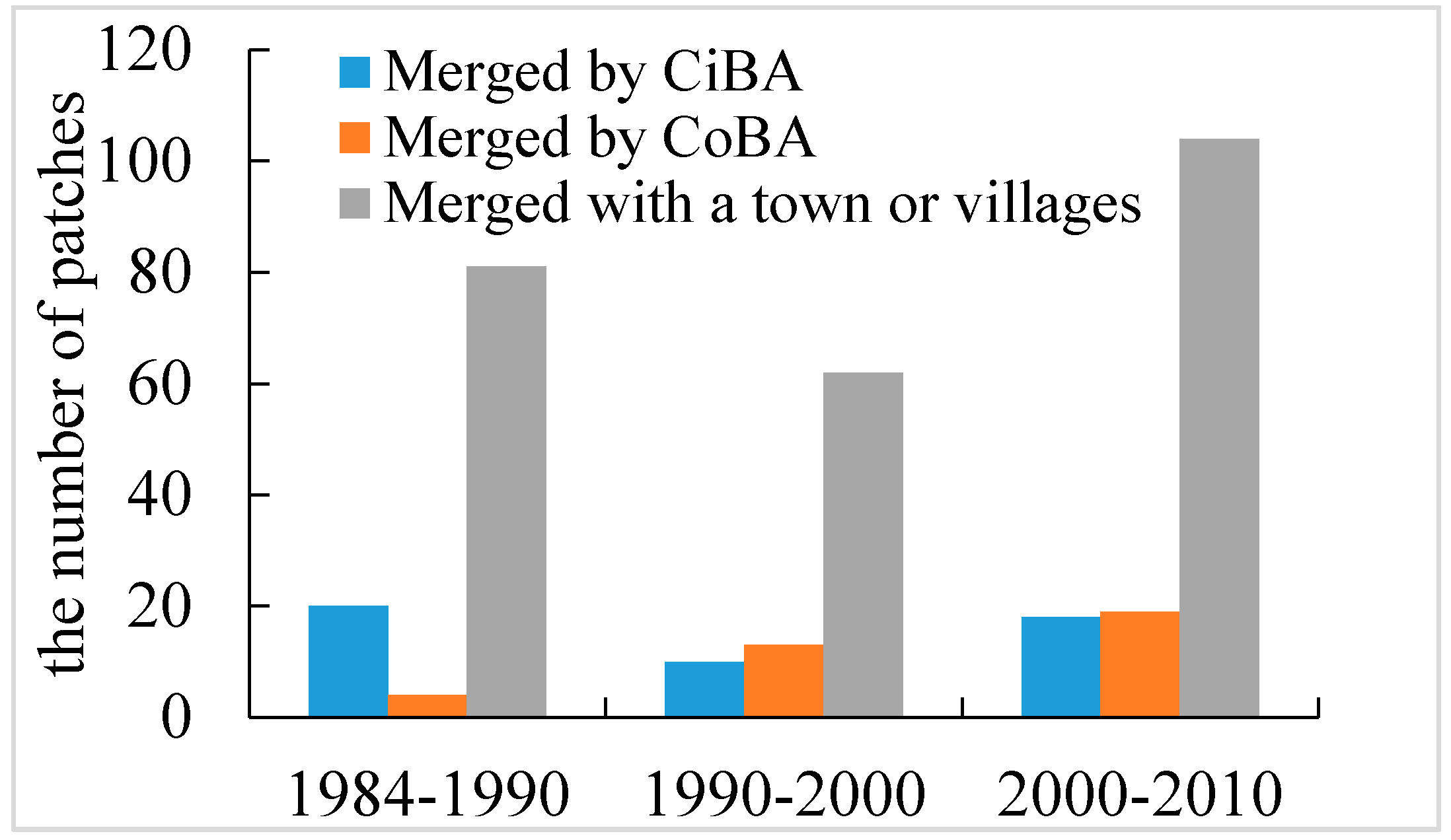
In this study, we developed a new approach to detect the changes of rural residential settlement at the village scale. In addition to the information about the changes of areas in rural settlements that most of the previous studies revealed [22,23,24], our approach allowed us to quantify the changes in the numbers of the rural settlements, and further classified the rural settlement changes into 5 types based on changes, including “no-change”, “totally lost”, “shrinking”, “expanding” and “merged”. Information provided by this approach enhanced our understanding of the changes of rural settlements during the process of rapid urbanization. For example, we found that from 1984 to 1990, merged villages were mostly merged into the city built-up area of Beijing, but the number of settlements that merged into county built-up areas (i.e., satellite cities) increased continuously since 1990 (Figure 5). These results reflected the changes of the urban development policy in Beijing, and more broadly, in China. Before 1990, the policy of developing big cities was implemented in China, but the policy was changed to coordinated development of small towns and cities, with medium-sized and large cities starting in 1990 [49,50,51].
Another example is classification of different types of villages based on their changes, which was not considered in the previous studies [4,52]. With this approach, we revealed that the total number of settlements that were totally lost or shrunken decreased sharply during the past 30 years, while that of settlements with no change and merged types both presented “U-shaped” increasing curves. In addition, most of the rural residential settlements with changes were spatially located in urban development areas, consisting of 67.32%, 70.24%, and 69.93% of all sampled settlements in Beijing in different time periods. While we only tested this approach in the Beijing metropolitan area, we would expect that this approach could be applied in other metropolitan areas for better understanding of changes in rural residential settlements and their associations with urbanization.
4.2. The Effects of Driving Forces on Changes Varied by Time
The observed changes in rural residential settlements in Beijing were affected by both topographical and distance factors, but their impacts changed through time and varied by types of change. For example, the settlements that were totally lost were affected by both topographical and distance factors, but settlements that were expanded or merged were mostly affected by distance factors. These results were consistent with previous findings that the topographical conditions such as elevation and slope increasingly played a less important role affecting where impervious surface expansion occurs, because the advancement of technology has greatly reduced the construction costs in areas with high elevation and steep slope [30,53]. Meanwhile, villages that were closer to cities or transportation typically experienced more development. This result is consistent with findings from many previous studies [2,54].
Additionally, distance to county (or satellite city) center and to provincial road showed increasing influence on settlement expansion through time compared to distance to railways or rail stations. This shift is due to the great changes in means of transportation. For instance, the railway passenger volume in Beijing has increased 3-fold from 38.77 million in 1984 to 126.09 million in 2014. In contrast, the highway passenger volume grew 16-fold from 32.87 million to 523.54 million in the same period [26].
4.3. Limitations and Future Research
The accurate mapping and identification of rural settlements is the basis for settlement change analysis. In order to better understand the change of rural settlement in Beijing over a long time series, we used Landsat TM images from 1984 to 2010 to obtain the rural residential settlements in this study. Although we employed the object-based classification approach to improve the classification accuracy [16], the use of the relatively coarse spatial resolution of 30 m is likely to miss some detailed information of fine-scale changes in rural settlements [43,55]. The availability of very high spatial resolution images with sub-meter spatial resolution, such as QuickBird, and Worldview image data, can provide data to detect fine-scale changes in rural settlements [4,52,56]. Analysis based on such data is highly desirable in future studies.
In addition, while the PCP of the multinomial logistic regressions (MLR) indicated acceptable performance of the models [47,48,57,58], the R2 values of these models were relatively low, which suggested that there are other factors affecting the change of village settlements that were not included. Including more socioeconomic driving factors—such as population, household income and education—could potentially improve the performance of these regression models.
5. Conclusions
Globally, urban expansion has resulted in dramatic changes in rural landscapes, which have marked social and eco-environmental consequences. Understanding how rural villages have changed over time and the drivers of change is crucially important to assess such consequences. Using remote sensing data to quantify the distribution of rural settlements and their changes has received increasing attention in the past three decades, but remains a challenge. This study presents a new approach that can identify five different types of changes at the individual village level by integrating remote sensing and GIS analyses, using multi-temporal Landsat TM image data. We applied this approach to quantify the spatiotemporal patterns of rural residential settlements in the Beijing metropolitan area from 1984 to 2010. We found: (1) 36% of the villages were lost, but the total area of developed lands in existing villages increased by 34%; (2) Changes were dominated by the type of ‘expansion’ in 1984–1990 (accounting for 43.42%) and 1990–2000 (56.21%). However, from 2000 to 2010, 49.73% of the villages remained unchanged; (3) both topographical factors and distance factors had significant effects on whether the villages changed or not, and the types of changes they had; but their impacts changed through time. The topographical driving factors showed decreasing effects on the loss of rural settlements, while distance factors had increasing impacts on settlement expansion and merging. Results from this study can enhance our understanding of the changes in rural residential settlements and their associations with urbanization in the Beijing metropolitan area. While only tested in Beijing, this approach can be applied in other metropolitan areas as well.
Acknowledgments
This research was funded by the National Natural Science Foundation of China (Grant No. 41422014 and 41590841), the project “Developing key technologies for establishing ecological security patterns at the Beijing-Tianjin-Hebei urban megaregion” of the National key research and development program (2016YFC0503004), the Key Research Program of Frontier Sciences, CAS (QYZDB-SSW-DQC034), the One Hundred Talents program and the strategic environmental assessment of key regions and industry development (2110203). We would like to thank Nicholas Weller at Arizona State University, whose comments helped improve the early draft of this manuscript.
Author Contributions
Weiqi Zhou and Kun Wang designed this research. Kun Wang, Weiqi Zhou, Hanmei Liang and Wenjuan Yu conducted the analysis. Kun Wang, Weiqi Zhou, Kaipeng Xu, Hanmei Liang, Wenjuan Yu, and Weifeng Li wrote the paper.
Conflicts of Interest
The authors declare that there is no conflict of interest.
References
- Gude, P.H.; Hansen, A.J.; Rasker, R.; Maxwell, B. Rates and drivers of rural residential development in the Greater Yellowstone. Landsc. Urban Plan. 2006, 77, 131–151. [Google Scholar] [CrossRef]
- Liu, Z.; Robinson, G.M. Residential development in the peri-urban fringe: The example of Adelaide, South Australia. Land Use Policy 2016, 57, 179–192. [Google Scholar] [CrossRef]
- Hersperger, A.M.; Bürgi, M. Going beyond landscape change description: Quantifying the importance of driving forces of landscape change in a Central Europe case study. Land Use Policy 2009, 26, 640–648. [Google Scholar] [CrossRef]
- Tan, M.; Li, X. The changing settlements in rural areas under urban pressure in China: Patterns, driving forces and policy implications. Landsc. Urban Plan. 2013, 120, 170–177. [Google Scholar] [CrossRef]
- Shan, Y. On extraction and fractal of urban and rural residential spatial pattern in developed area. Acta Geogr. Sin. 2000, 6, 671–678. [Google Scholar]
- McHale, M.; Pickett, S.; Barbosa, O.; Bunn, D.; Cadenasso, M.; Childers, D.; Gartin, M.; Hess, G.; Iwaniec, D.; McPhearson, T.; et al. The New Global Urban Realm: Complex, Connected, Diffuse, and Diverse Social-Ecological Systems. Sustainability 2015, 7, 5211–5240. [Google Scholar] [CrossRef]
- Pickett, S.T.A.; Zhou, W. Global urbanization as a shifting context for applying ecological science toward the sustainable city. Ecosyst. Health Sustain. 2015, 1, 5. [Google Scholar] [CrossRef]
- Kauppi, P.E.; Ausubel, J.H.; Fang, J.; Mather, A.S.; Sedjo, R.A.; Waggoner, P.E. Returning forests analyzed with the forest identity. Proc. Natl. Acad. Sci. USA 2006, 103, 17574–17579. [Google Scholar] [CrossRef] [PubMed]
- Shi, L.; Zhao, S.; Tang, Z.; Fang, J. The changes in China’s forests: An analysis using the forest identity. PLoS ONE 2011, 6, e207786. [Google Scholar] [CrossRef] [PubMed]
- Sitzia, T.; Semenzato, P.; Trentanovi, G. Natural reforestation is changing spatial patterns of rural mountain and hill landscapes: A global overview. For. Ecol. Manag. 2010, 259, 1354–1362. [Google Scholar] [CrossRef]
- Sanchez-Cuervo, A.M.; Aide, T.M.; Clark, M.L.; Etter, A. Land cover change in Colombia: Surprising forest recovery trends between 2001 and 2010. PLoS ONE 2012, 7, e439438. [Google Scholar] [CrossRef] [PubMed]
- Zhou, W.; Qian, Y.; Li, X.; Li, W.; Han, L. Relationships between land cover and the surface urban heat island: Seasonal variability and effects of spatial and thematic resolution of land cover data on predicting land surface temperatures. Landsc. Ecol. 2014, 29, 153–167. [Google Scholar] [CrossRef]
- Zhou, W.; Huang, G.; Pickett, S.T.A.; Cadenasso, M.L. 90 years of forest cover change in an urbanizing watershed: Spatial and temporal dynamics. Landsc. Ecol. 2011, 26, 645–659. [Google Scholar] [CrossRef]
- Comber, A.; Balzter, H.; Cole, B.; Fisher, P.; Johnson, S.; Ogutu, B. Methods to quantify regional differences in land cover change. Remote Sens. Basel 2016, 8, 176. [Google Scholar] [CrossRef]
- Tewkesbury, A.P.; Comber, A.J.; Tate, N.J.; Lamb, A.; Fisher, P.F. A critical synthesis of remotely sensed optical image change detection techniques. Remote Sens. Environ. 2015, 160, 1–14. [Google Scholar] [CrossRef]
- Yu, W.; Zhou, W.; Qian, Y.; Yan, J. A new approach for land cover classification and change analysis: Integrating backdating and an object-based method. Remote Sens. Environ. 2016, 177, 37–47. [Google Scholar] [CrossRef]
- Tsutsumida, N.; Comber, A.; Barrett, K.; Saizen, I.; Rustiadi, E. Sub-pixel classification of MODIS EVI for annual mappings of impervious surface areas. Remote Sens. 2016, 8, 143. [Google Scholar] [CrossRef]
- Deadman, P.; Brown, R.D.; Gimblett, H.R. Modelling rural residential settlement patterns with Cellular Automata. J. Environ. Manag. 1993, 37, 147–160. [Google Scholar] [CrossRef]
- Tian, G.; Yang, Z.; Zhang, Y. The spatio-temporal dynamic pattern of rural residential land in China in the 1990s using landsat TM images and GIS. Environ. Manag. 2007, 40, 803–813. [Google Scholar] [CrossRef] [PubMed]
- Tian, G.; Liu, J.; Zhuang, D. The temporal-spatial characteristics of rural residential land in China in the 1990s. Acta Geogr. Sin. 2003, 58, 651–658. [Google Scholar]
- Long, H.; Heilig, G.K.; Li, X.; Zhang, M. Socio-economic development and land-use change: Analysis of rural housing land transition in the transect of the Yangtse River, China. Land Use Policy 2007, 24, 141–153. [Google Scholar] [CrossRef]
- Cai, W.; Tang, H.; Chen, Y.; Zhang, F. Landscape Pattern of Rural Residential Areas in Yellow River Delta in Recent 20 Years. Resour. Sci. 2004, 26, 89–97. [Google Scholar]
- Li, H.; Zhang, X.; Wu, J.; Zhu, B. Spatial pattern and its driving mechanism of rural settlements in Southern Jiangsu. Sci. Geogr. Sin. 2014, 34, 438–446. [Google Scholar]
- Hu, X.; Yang, G.; Zhang, X.; Qiu, J. The change of land use for rural residency and the driving forces: A case study in Xiantao city, Hubei Province. Resour. Sci. 2007, 29, 191–197. [Google Scholar]
- Plieninger, T.; Draux, H.; Fagerholm, N.; Bieling, C.; Bürgi, M.; Kizos, T.; Kuemmerle, T.; Primdahl, J.; Verburg, P.H. The driving forces of landscape change in Europe: A systematic review of the evidence. Land Use Policy 2016, 57, 204–214. [Google Scholar] [CrossRef]
- Beijing Bureau of Statistics. Statistical Yearbook of Beijing; China Statistic Press: Beijing, China, 2015.
- Xu, Y.; Shen, H.; Gan, G.; Guo, T. Rural residential land use change and its correlative model with population in Fengtai district of Beijing. Acta Geogr. Sin. 2002, 57, 569–576. [Google Scholar]
- Tian, G.; Qiao, Z.; Zhang, Y. The investigation of relationship between rural settlement density, size, spatial distribution and its geophysical parameters of China using Landsat TM images. Ecol. Model. 2012, 231, 25–36. [Google Scholar] [CrossRef]
- Baatz, M.; Schäpe, A. Multiresolution segmentation: An optimization approach for high quality multi-scale image segmentation. Angew. Geogr. Informationsverarb. XII 2000, 58, 12–23. [Google Scholar]
- Li, X.; Zhou, W.; Ouyang, Z. Forty years of urban expansion in Beijing: What is the relative importance of physical, socioeconomic, and neighborhood factors? Appl. Geogr. 2013, 38, 1–10. [Google Scholar] [CrossRef]
- Steen-Adams, M.M.; Mladenoff, D.J.; Langston, N.E.; Liu, F.; Zhu, J. Influence of biophysical factors and differences in Ojibwe reservation versus Euro-American social histories on forest landscape change in northern Wisconsin, USA. Landsc. Ecol. 2011, 26, 1165–1178. [Google Scholar] [CrossRef]
- Crk, T.; Uriarte, M.; Corsi, F.; Flynn, D. Forest recovery in a tropical landscape: what is the relative importance of biophysical, socioeconomic, and landscape variables? Landsc. Ecol. 2009, 24, 629–642. [Google Scholar] [CrossRef]
- Qian, Y.; Zhou, W.; Li, W.; Han, L. Understanding the dynamic of greenspace in the urbanized area of Beijing based on high resolution satellite images. Urban For. Urban Green. 2015, 14, 39–47. [Google Scholar] [CrossRef]
- Lillesand, T.M.; Kiefer, R.W.; Chipman, J.W. Remote Sensing and Image Interpretation; John Wiley & Sons: Hoboken, NJ, USA, 2004. [Google Scholar]
- Bürgi, M.; Hersperger, A.M.; Schneeberger, N. Driving forces of landscape change—Current and new directions. Landsc. Ecol. 2004, 19, 857–868. [Google Scholar] [CrossRef]
- Seto, K.C.; Fragkias, M.; Guneralp, B.; Reilly, M.K. A meta-analysis of global urban land expansion. PLoS ONE 2011, 6, e23777. [Google Scholar] [CrossRef] [PubMed]
- Wu, Y.; Li, S.; Yu, S. Monitoring urban expansion and its effects on land use and land cover changes in Guangzhou city, China. Environ. Monit. Assess. 2016, 188, 54. [Google Scholar] [CrossRef] [PubMed]
- Batisani, N.; Yarnal, B. Urban expansion in Centre County, Pennsylvania: Spatial dynamics and landscape transformations. Appl. Geogr. 2009, 29, 235–249. [Google Scholar] [CrossRef]
- Dendoncker, N.; Rounsevell, M.; Bogaert, P. Spatial analysis and modelling of land use distributions in Belgium. Comput. Environ. Urban Syst. 2007, 31, 188–205. [Google Scholar] [CrossRef]
- Luo, J.; Wei, Y.H. D. Modeling spatial variations of urban growth patterns in Chinese cities: The case of Nanjing. Landsc. Urban Plan. 2009, 91, 51–64. [Google Scholar] [CrossRef]
- Reilly, M.K.; O Mara, M.P.; Seto, K.C. From Bangalore to the Bay Area: Comparing transportation and activity accessibility as drivers of urban growth. Landsc. Urban Plan. 2009, 92, 24–33. [Google Scholar] [CrossRef]
- Zank, B.; Bagstad, K.J.; Voigt, B.; Villa, F. Modeling the effects of urban expansion on natural capital stocks and ecosystem service flows: A case study in the Puget Sound, Washington, USA. Landsc. Urban Plan. 2016, 149, 31–42. [Google Scholar] [CrossRef]
- Kuang, W.; Liu, J.; Dong, J.; Chi, W.; Zhang, C. The rapid and massive urban and industrial land expansions in China between 1990 and 2010: A CLUD-based analysis of their trajectories, patterns, and drivers. Landsc. Urban Plan. 2016, 145, 21–33. [Google Scholar] [CrossRef]
- Long, Y.; Gu, Y.; Han, H. Spatiotemporal heterogeneity of urban planning implementation effectiveness: Evidence from five urban master plans of Beijing. Landsc. Urban Plan. 2012, 108, 103–111. [Google Scholar] [CrossRef]
- Dubovyk, O.; Sliuzas, R.; Flacke, J. Spatio-temporal modelling of informal settlement development in Sancaktepe district, Istanbul, Turkey. ISPRS J. Photogramm. Remote Sens. 2011, 66, 235–246. [Google Scholar] [CrossRef]
- Ledolter, J. Multinomial Logistic Regression. In Data Mining and Business Analytics with R; John Wiley & Sons, Inc.: Somerset, NJ, USA, 2013; pp. 132–149. [Google Scholar]
- Zhang, W. Advanced SPSS statistical Analysis Tutorial; Higher Education Press: Beijing, China, 2004. [Google Scholar]
- Shu, B.R.; Zhang, H.H.; Li, Y.L.; Qu, Y.; Chen, L.H. Spatiotemporal variation analysis of driving forces of urban land spatial expansion using logistic regression: A case study of port towns in Taicang City, China. Habit. Int. 2014, 43, 181–190. [Google Scholar] [CrossRef]
- Song, W.; Pijanowski, B.C.; Tayyebi, A. Urban expansion and its consumption of high-quality farmland in Beijing, China. Ecol. Indic. 2015, 54, 60–70. [Google Scholar] [CrossRef]
- Liu, Y.; Yue, W.; Fan, P.; Song, Y. Suburban residential development in the era of market-oriented land reform: The case of Hangzhou, China. Land Use Policy. 2015, 42, 233–243. [Google Scholar] [CrossRef]
- Fang, C. A review of Chinese urban development policy, emerging patterns and future adjustments. Geograp. Res. 2014, 33, 674–686. [Google Scholar]
- Lu, D.; Tian, H.; Zhou, G.; Ge, H. Regional mapping of human settlements in southeastern China with multisensor remotely sensed data. Remote Sens. Environ. 2008, 112, 3668–3679. [Google Scholar] [CrossRef]
- Ye, Y.; Zhang, H.; Liu, K.; Wu, Q. Research on the influence of site factors on the expansion of construction land in the Pearl River Delta, China: By using GIS and remote sensing. Int. J. Appl. Earth Obs. 2013, 21, 366–373. [Google Scholar] [CrossRef]
- Ibrahim Mahmoud, M.; Duker, A.; Conrad, C.; Thiel, M.; Shaba Ahmad, H. Analysis of settlement expansion and urban growth modelling using geoinformation for assessing potential impacts of urbanization on climate in Abuja City, Nigeria. Remote Sens.-Basel 2016, 8, 220. [Google Scholar] [CrossRef]
- Myint, S.W.; Gober, P.; Brazel, A.; Grossman-Clarke, S.; Weng, Q. Per-pixel vs. object-based classification of urban land cover extraction using high spatial resolution imagery. Remote Sens. Environ. 2011, 115, 1145–1161. [Google Scholar] [CrossRef]
- Guo, W.; Lu, D.; Wu, Y.; Zhang, J. Mapping Impervious Surface Distribution with Integration of SNNP VIIRS-DNB and MODIS NDVI Data. Remote Sens. 2015, 7, 12459–12477. [Google Scholar] [CrossRef]
- Tian, Y.; Xu, Y.; Guo, H.; Wu, Y. Simulation of farmland use pattern in Zhangjiakou based on multinomial logistic regression model. Res. Sci. 2012, 34, 1493–1499. [Google Scholar]
- Pontius, R.G., Jr.; Schneider, L.C. Land-cover change model validation by an ROC method for the Ipswich watershed, Massachusetts, USA. Agri. Ecosyst. Environ. 2001, 85, 239–248. [Google Scholar] [CrossRef]
Figure 1.
The study area–Beijing metropolitan area–includes four different types of functional zones. The City Built-up Area (CiBA) and County Built-up Area (CoBA) in Beijing in 2010 are shown in this map from Baidu MapTM, a popular map service in China similar to Google Maps™.
Figure 1.
The study area–Beijing metropolitan area–includes four different types of functional zones. The City Built-up Area (CiBA) and County Built-up Area (CoBA) in Beijing in 2010 are shown in this map from Baidu MapTM, a popular map service in China similar to Google Maps™.
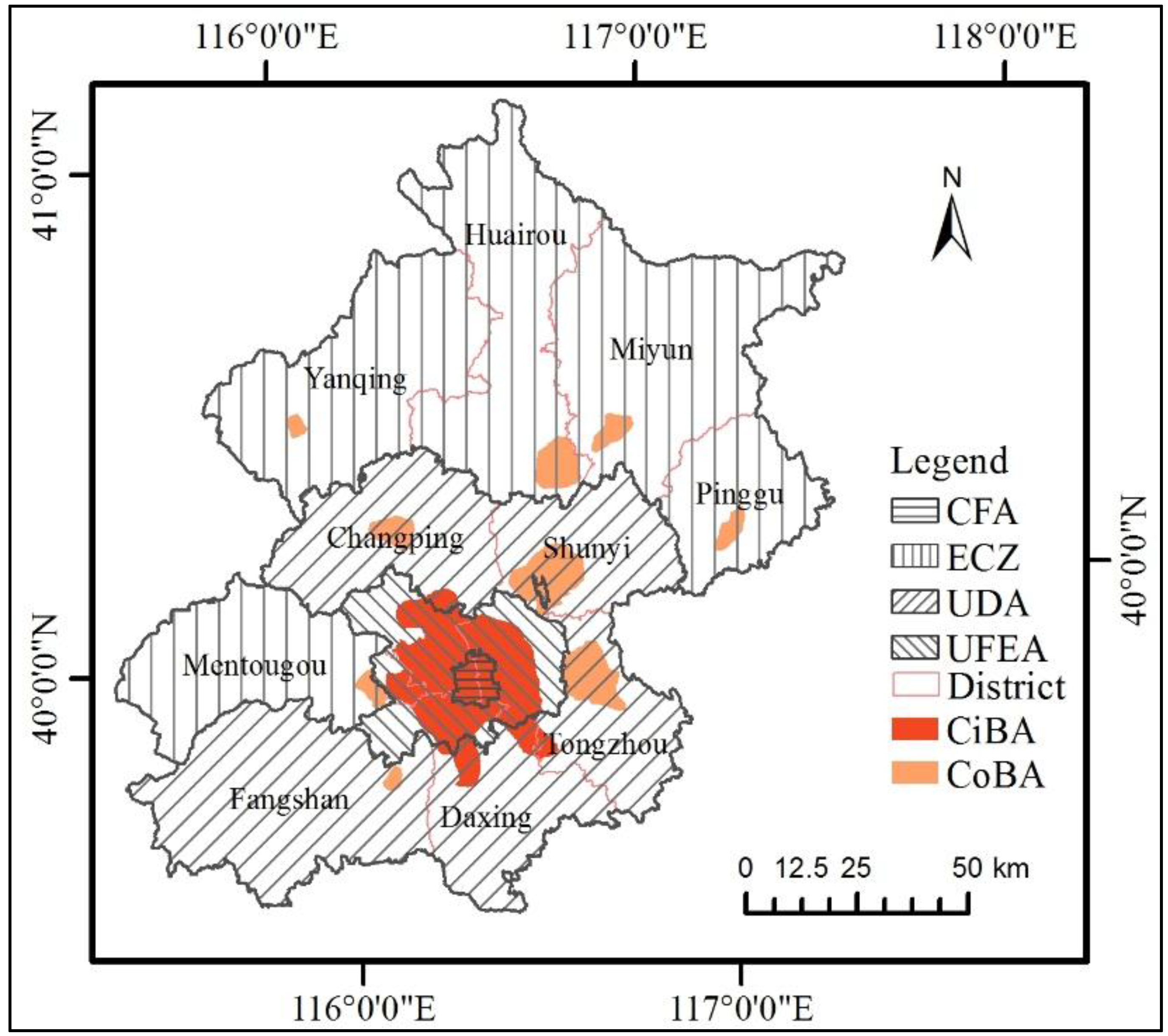
Figure 2.
Flow chart of change detection and driving analysis of rural settlements.

Figure 3.
The spatial distribution of the selected driving factors for 1984–1990.
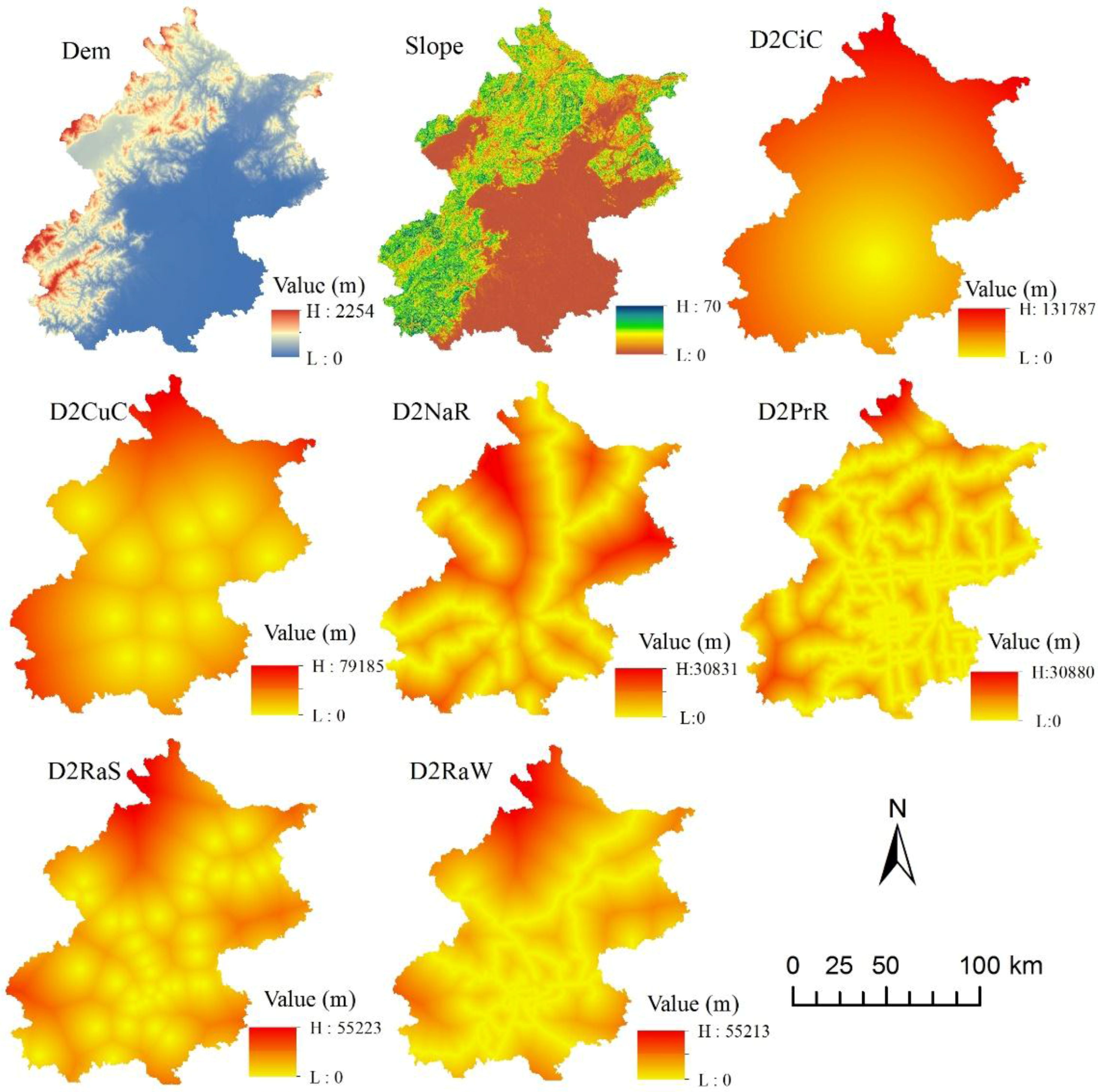
Figure 4.
The spatial distribution of sampled settlements with different types of changes in Beijing.
Figure 4.
The spatial distribution of sampled settlements with different types of changes in Beijing.
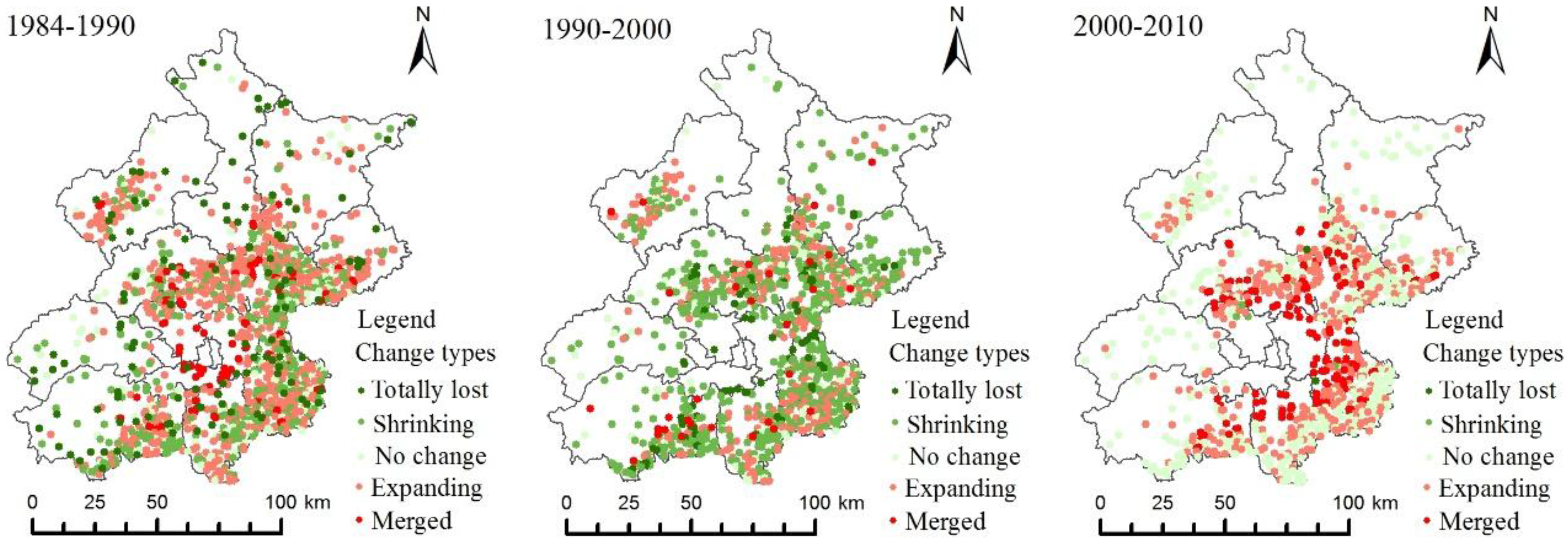
Figure 5.
The variation of settlement in different merge types.


Table 1.
The change types of rural residential settlement.
| Change Classes | Change Types | Sub-Change Types | Description | Examples | |
|---|---|---|---|---|---|
| Time I (Grey Polygon) | Time II (Red Polygon ) | ||||
| No change | No change | The change in size is less than 3600 m2. | a  | ||
| Change | Totally lost | The patch rural settlement is totally lost. | b  | ||
| Shrinking | Part of the patch is removed, and the size of the patch becomes smaller. | c  | |||
| Expanding | The patch of rural settlement becomes larger. | d  | |||
| Merged | Merged by CiBA | The patch of rural settlement is merged with the city built-up area of Beijing. | e  | ||
| Merged by CoBA | The patch of rural settlement is merged with the county built-up area. | f  | |||
| Merged with a town or villages | The patch of rural settlement is merged with a town center or other rural settlement. | g  | |||
Table 2.
List of the selected drivers of rural residential settlement change.
| Category | Variables | Description |
|---|---|---|
| Topographical factors | Dem (m) | Elevation |
| Slope | Slope | |
| Distance factors | D2CiC (m) | Distance to city center |
| D2CoC (m) | Distance to county center (satellite city) | |
| D2RaS (m) | Distance to rail station | |
| D2RaW (m) | Distance to railway | |
| D2NaR (m) | Distance to national road | |
| D2PrR (m) | Distance to provincial road |
Table 3.
The numbers of villages and total areas of developed land in different time slices and their changes.
Table 3.
The numbers of villages and total areas of developed land in different time slices and their changes.
| Year | Total Number | Total Area (km2) | Period | Changes in Number | Changes in Total Area (km2) |
|---|---|---|---|---|---|
| 1984 | 1276 | 379 | |||
| 1990 | 1055 | 385 | 1984–1990 | −221 | 6 |
| 2000 | 941 | 422 | 1990–2000 | −114 | 37 |
| 2010 | 812 | 507 | 2000–2010 | −129 | 85 |
Table 4.
The numbers of villages in different types of change.
| Change Types | 1984–1990 | 1990–2000 | 2000–2010 | |
|---|---|---|---|---|
| No Change | 132 | 94 | 468 | |
| Change | Totally lost | 125 | 30 | 2 |
| Shrinking | 359 | 253 | 5 | |
| Expanding | 554 | 593 | 325 | |
| Merged | 106 | 85 | 141 | |
Table 5.
The number of settlements in different change types in different areas.
| Period | 1984–1990 | 1990–2000 | 2000–2010 | |||||||
|---|---|---|---|---|---|---|---|---|---|---|
| Functional zones | UFEA | UDA | ECZ | UFEA | UDA | ECZ | UFEA | UDA | ECZ | |
| No change | 1 | 93 | 38 | 2 | 61 | 31 | 6 | 305 | 157 | |
| Change | Totally lost | 7 | 65 | 53 | 2 | 24 | 4 | 1 | 1 | |
| Shrinking | 18 | 278 | 63 | 4 | 179 | 70 | 3 | 2 | ||
| Expanding | 33 | 358 | 163 | 37 | 409 | 147 | 13 | 239 | 73 | |
| Merged | 31 | 65 | 10 | 8 | 68 | 9 | 18 | 111 | 12 | |
| Total villages in each zone | 90 | 859 | 327 | 53 | 741 | 261 | 40 | 658 | 243 | |
| Proportion (%) | 7.05 | 67.32 | 25.63 | 5.02 | 70.24 | 24.74 | 4.25 | 69.93 | 25.82 | |
Table 6.
The area changes of settlements in urban development areas.
| Types | 1984–1990 | 1990–2000 | 2000–2010 | |||
|---|---|---|---|---|---|---|
| Change Area (km2) | Proportion | Change Area (km2) | Proportion | Change Area (km2) | Proportion | |
| Totally lost | −16.32 | 75.18% | −13.46 | 75.51% | −0.55 | 48.84% |
| Shrinking | −16.46 | 71.95% | −15.46 | 85.38% | −0.17 | 46.35% |
| Expanding | 82.72 | 53.79% | 82.83 | 58.51% | 190.99 | 86.98% |
Table 7.
The effects of driving factors on the changes of rural settlements.
| Period | Variables | Totally Lost | Shrinking | Expanding | Merged | ||||
|---|---|---|---|---|---|---|---|---|---|
| β | OR | β | OR | β | OR | β | OR | ||
| 1984–1990 | Dem | 0.987 | 2.684 | −0.412 | 0.662 | −0.051 | 0.951 | 0.098 | 1.102 |
| Slope | 4.026 * | 56.010 | 0.161 | 1.175 | −4.642 * | 0.010 | −5.313 | 0.005 | |
| D2CiC | 0.260 | 1.297 | −1.591 | 0.204 | 0.533 | 1.704 | −4.660 ** | 0.009 | |
| D2CoC | −0.312 | 0.732 | 0.181 | 1.199 | −1.119 | 0.327 | −4.332 * | 0.013 | |
| D2RaS | −5.768 ** | 0.003 | −3.525 * | 0.029 | −4.157 * | 0.016 | −1.206 | 0.299 | |
| D2RaW | 4.497 * | 89.719 | 1.921 | 6.828 | 2.397 | 10.994 | −3.282 | 0.038 | |
| D2NaR | 0.143 | 1.154 | 1.205 * | 3.338 | 0.865 | 2.375 | 0.077 | 1.080 | |
| D2PrR | −0.641 | 0.527 | 1.674 | 5.332 | −0.850 | 0.427 | −5.701 ** | 0.003 | |
| 1990–2000 | Dem | 0.599 | 1.820 | 1.754 | 5.780 | −0.024 | 0.976 | −4.251 | 0.014 |
| Slope | −0.183 | 0.833 | −9.391 ** | 0.000 | 0.200 | 1.221 | −3.143 | 0.043 | |
| D2CiC | −1.138 | 0.320 | −0.667 | 0.513 | −0.872 | 0.418 | −2.129 | 0.119 | |
| D2CoC | −0.297 | 0.743 | −0.114 | 0.892 | −1.128 | 0.324 | −2.142 | 0.117 | |
| D2RaS | −7.340 ** | 0.001 | −4.403 ** | 0.012 | −5.567 ** | 0.004 | −8.677 ** | 0.000 | |
| D2RaW | 1.816 | 6.150 | 2.076 | 7.970 | 4.535 ** | 93.190 | 3.167 | 23.746 | |
| D2NaR | 1.428 | 4.169 | 0.540 | 1.715 | 1.414 * | 4.114 | −0.123 | 0.884 | |
| D2PrR | 0.962 | 2.617 | −1.063 | 0.345 | −0.597 | 0.550 | −4.567 * | 0.010 | |
| 200–2010 | Dem | −0.414 | 0.661 | −2.395 | 0.091 | ||||
| Slope | −0.477 | 0.621 | −3.206 | 0.041 | |||||
| D2CiC | −2.345 ** | 0.096 | −10.319 ** | 0.000 | |||||
| D2CoC | −3.105 ** | 0.045 | −12.153 ** | 0.000 | |||||
| D2RaS | −0.798 | 0.450 | 5.854 ** | 348.475 | |||||
| D2RaW | 0.622 | 1.862 | −2.828 | 0.059 | |||||
| D2NaR | −0.455 | 0.634 | −1.364 * | 0.256 | |||||
| D2PrR | −2.783 ** | 0.062 | −4.413 ** | 0.012 | |||||
Reference category is “no change”, OR is the relative odd’s ratio, * p < 0.05, ** p < 0.01. Red means significant positive effect, while green means significant negative effect.
© 2017 by the authors. Licensee MDPI, Basel, Switzerland. This article is an open access article distributed under the terms and conditions of the Creative Commons Attribution (CC BY) license (http://creativecommons.org/licenses/by/4.0/).
Share and Cite
MDPI and ACS Style
Wang, K.; Zhou, W.; Xu, K.; Liang, H.; Yu, W.; Li, W. Quantifying Changes of Villages in the Urbanizing Beijing Metropolitan Region: Integrating Remote Sensing and GIS Analysis. Remote Sens. 2017, 9, 448. https://doi.org/10.3390/rs9050448
AMA Style
Wang K, Zhou W, Xu K, Liang H, Yu W, Li W. Quantifying Changes of Villages in the Urbanizing Beijing Metropolitan Region: Integrating Remote Sensing and GIS Analysis. Remote Sensing. 2017; 9(5):448. https://doi.org/10.3390/rs9050448
Chicago/Turabian StyleWang, Kun, Weiqi Zhou, Kaipeng Xu, Hanmei Liang, Wenjuan Yu, and Weifeng Li. 2017. "Quantifying Changes of Villages in the Urbanizing Beijing Metropolitan Region: Integrating Remote Sensing and GIS Analysis" Remote Sensing 9, no. 5: 448. https://doi.org/10.3390/rs9050448
Note that from the first issue of 2016, this journal uses article numbers instead of page numbers. See further details here.