Article

Land Surface Temperature and Emissivity Retrieval from Field-Measured Hyperspectral Thermal Infrared Data Using Wavelet Transform

1
University of Chinese Academy of Sciences, Beijing 100049, China
2
State Key Laboratory of Resources and Environment Information System, Institute of Geographic Sciences and Natural Resources Research, Chinese Academy of Sciences, Beijing 100101, China
3
Jiangsu Center for Collaborative Innovation in Geographical Information Resource Development and Application, Nanjing 210023, China
4
Key Laboratory of Quantitative Remote Sensing Information Technology, Academy of Opto-Electronics, Chinese Academy of Sciences, Beijing 100094, China
5
Xinjiang Institute of Ecology and Geography, Chinese Academy of Sciences, Urumqi 830011, China
6
ICube, UdS, CNRS, 300 Bld Sébastien Brant, CS10413, 67412 Illkirch, France
*
Authors to whom correspondence should be addressed.
Remote Sens. 2017, 9(5), 454; https://doi.org/10.3390/rs9050454
Submission received: 9 March 2017 / Revised: 21 April 2017 / Accepted: 3 May 2017 / Published: 7 May 2017

Abstract

:
Currently, the main difficulty in separating the land surface temperature (LST) and land surface emissivity (LSE) from field-measured hyperspectral Thermal Infrared (TIR) data lies in solving the radiative transfer equation (RTE). Based on the theory of wavelet transform (WT), this paper proposes a method for accurately and effectively separating LSTs and LSEs from field-measured hyperspectral TIR data. We show that the number of unknowns in the RTE can be reduced by decomposing and reconstructing the LSE spectrum, thus making the RTE solvable. The final results show that the errors introduced by WT are negligible. In addition, the proposed method usually achieves a greater accuracy in a wet-warm atmosphere than that in a dry-cold atmosphere. For the results under instrument noise conditions (NE∆T = 0.2 K), the overall accuracy of the LST is approximately 0.1–0.3 K, while the Root Mean Square Error (RMSE) of the LSEs is less than 0.01. In contrast to the effects of instrument noise, our method is quite insensitive to noises from atmospheric downwelling radiance, and all the RMSEs of our method are approximately zero for both the LSTs and the LSEs. When we used field-measured data to better evaluate our method’s performance, the results showed that the RMSEs of the LSTs and LSEs were approximately 1.1 K and 0.01, respectively. The results from both simulated data and field-measured data demonstrate that our method is promising for decreasing the number of unknowns in the RTE. Furthermore, the proposed method overcomes some known limitations of current algorithms, such as singular values and the loss of continuity in the spectrum of the retrieved LSEs.

Graphical Abstract

1. Introduction

Land surface temperature (LST) and land surface emissivity (LSE) are two key variables in quantitative remote sensing that play roles in both environmental and geological fields [1,2,3]. For example, having an accurate LST map is an important input parameter for building and driving climate models at various scales [4]. In contrast, LSE can be regarded as a critical indicator of the structure and composition of the Earth’s surface and is particularly useful in mineralogical and geological mapping, as well as in land surface classifications [5,6,7].
In recent decades, researchers have made great efforts to estimate the LST and LSE from remote sensed thermal infrared (TIR) data. One of the key problems, as Realmuto mentioned in 1990, is to solve the ill-posed radiation transfer equation (RTE) to separate the land surface temperature and emissivity [8]. That is, there are always N spectral measurements of radiance to solve N + 1 unknowns (N LSEs, one LST). Moreover, the unknowns increase due to atmospheric presence. Although many methods to estimate LST and LSE have been developed from multispectral TIR data, such as the split-window algorithm and Day/Night algorithm for Moderate Resolution Imaging Spectroradiometer (MODIS) data and the Temperature/Emissivity Separation method for Advanced Spaceborne Thermal Emission and Reflection Radiometer (ASTER) data [9,10,11], they typically require various assumptions to be made about LSE, such as a certain emissivity at a particular wavelength, a fixed maximum emissivity, an approximation of the Planck function, and so forth. [5,8,12,13,14,15,16].
The increasing use of hyperspectral imagers [17,18,19,20] provides a new direction for retrieving the LST and LSE by using a larger number of TIR channels. Several algorithms have been proposed in recent years that build some constraints or adopt some simple assumptions. For example, based on the fact that the typical LSE spectrum is smoother than the LSE with atmospheric features, Borel proposed the Iterative Spectrally Smooth Temperature and Emissivity Separation (ISSTES) algorithm to simultaneously retrieve the LST and LSE [21]. Inspired by the theory behind the ISSTES algorithm, Wang et al. proposed a Linear Emissivity Constraint Temperature and Emissivity Separation (LECTES) algorithm by using several linear functions to reshape the LSE spectrum [22]. Other algorithms for hyperspectral TIR data include the Downwelling Radiance Residual Index (DRRI) algorithm, the Stepwise Refining Temperature and Emissivity Separation (SRTES) algorithm, and the Fast Line-of-Sight Atmospheric Analysis of Spectral Hypecubes Infrared (FLASHH-IR) method, etc. [23,24,25,26,27,28].
Among these algorithms, the most common is the ISSTES algorithm; however, the key problem of the ISSTES is the singular problem that is caused by using the simple inversion of the RTE to estimate the LSEs [21]. Consequently, extreme LSE values will be found when the LST is close to the effective air temperature. In addition, the ISSTES algorithm requires the assumption of a smooth LSE spectrum [22]. Although the singular problem can be reduced to some extent in LECTES, it has been reported that the LECTES algorithm loses the continuity of the LSE spectrum, particularly for surfaces with a fluctuating spectrum, and the LSE shape assumption is still required [22,26]. Similar problems also exist in other algorithms. To develop a more efficient method to accurately retrieve the LST and LSE from hyperspectral TIR data, this paper proposes a Wavelet-transformed Temperature and Emissivity Separation (WTTES) algorithm based on the wavelet transform theory. Because the atmospheric influence can be corrected by several methods such as the Radiative Transfer Model (RTM) method, Autonomous Atmospheric Compensation (AAC) method, In-Scene Atmospheric Compensation (ISAC) method, and Water Vapor Scale (WVS) method [29,30,31,32,33,34], this work mainly focuses on retrieving the LST and LSE from field-measured TIR data; airborne and satellite data will be addressed in future work. The sections in this paper are organized as follows: Section 2 briefly explains the basic theory and describes the details of our method and the experimental data used in this paper. Section 3 provides the results of the experiments and discussions. Section 4 presents the conclusions and future work.

2. Methodology and Data

2.1. Radiative Transfer Theory

Based on Wien’s Law, the radiant contribution of the Sun is small in the TIR range and can be ignored, without introducing obvious errors. Therefore, under clear conditions, the RTE at ground level for each TIR channel can be described in [2,3]:
L i , g = ε i , s B i ( T s ) + ( 1 ε i , s ) L i , d o w n
where i denotes the TIR channel; Li,g is the radiance measured at ground level; εi,s is the land surface emissivity; Ts is the land surface temperature; Li,down is the atmospheric downwelling radiance; and Bi(Ts) is the Planck Function with a temperature of Ts, whose formulation is as follows [2,3]:
B i ( T ) = C 1 λ i 5 ( e C 2 λ i T 1 ) 1
where λi is the wavelength in μm; and C1 and C2 are the constants, respectively. (C1 = 1.191 × 10⁸ W∙µm4∙sr−1∙m−2 and C2 = 1.439 × 104 µm∙K).
From this RTE, it is obvious that the equation is still ill-posed, even if the atmospheric downwelling radiance is known in advance. That is, for the observed radiance at N channels, there are always N + 1 (N channel LSE and 1 LST) unknowns. These unknowns form the key problem in retrieving LSTs and LSEs.

2.2. Wavelet Transform Method for Temperature and Emissivity Separation (WTTES)

Wavelet Transform (WT) is a tool for dividing a dataset, function, or operator into different frequency components: high- and low-frequency wavelet coefficients. In the wavelet domain, the high-frequency wavelet coefficients of a continuum time (space) series signal usually represent noise, while the low-frequency wavelet coefficients contain the bulk of the information in the original signal [35,36,37,38]. Based on this theory, the LSEs can then be recovered from the low-frequency wavelet coefficients alone.
ε r = D W T 1 ( C a , d b , n )
where εr represents the recovered LSEs and DWT−1 is the inversion of the discrete wavelet transform function. Because the LSEs are always obtained from certain channels, a discrete wavelet transform is used instead of a continuum wavelet transform. Ca represents the low-frequency wavelet coefficients, db is the selected wavelet, and n denotes the number of wavelet transform levels. Ca can be estimated from the original LSEs as follows:
[ C a , C d ] = D W T ( ε s , d b , n )
where Cd represents the high-frequency wavelet coefficients and εs denotes the original LSEs.
Here, by substituting (3) into (1), the at-ground radiances Lg can be then rewritten, as shown below:
L g = D W T 1 ( C a , d b , n ) B ( T s ) + ( 1 D W T 1 ( C a , d b , n ) ) L d o w n
Clearly, by using the wavelet transform on LSEs, the separation of temperature and emissivity is now converted to one of retrieving the Ts and the low-frequency wavelet coefficients (Ca) of LSEs; thus obviously reducing the unknowns in the RTE. For example, for N channels, there are only N/2 + 1 unknowns, N/2 Ca and 1 LST, in (5), when n = 1. The number of unknowns will be reduced further if a higher wavelet level is adopted.
However, because the analytical expression of the LST and Ca cannot be deduced, an iterative solution is used to determine the unknowns in (5) and minimize the cost function defined in (6), which is based on the fact that the optimal LSTs and LSEs always correspond to the least difference between the estimated and measured radiance [38]:
E c o s t = σ ( L g ' L g )
where Ecost is the cost function, σ is the standard deviation, L’g is the estimated radiance at ground level, and Lg is the measured radiance at ground level.
The detailed steps required to separate the LSTs and LSEs from field-measured hyperspectra TIR data are given below: First, an initial LST must be given, such as the maximum of the LSTs calculated with a constant LSE using the normalization emissivity method. Next, an initial LSE spectrum is obtained using the inversion of the RTE with the estimated initial LST. Subsequently, the low-frequency wavelet coefficients (Ca) of the LSEs can be acquired using the wavelet transform in (4). The Newton Method is then used to solve the nonlinear equation in (5). That is, the initial LST and Ca are iteratively adjusted according to the calculated value of Ecost defined in (6). After the Ecost attains its minimum value, the iterative calculation is terminated, and the current LST and Ca are regarded as the optimal values. The final LSEs can be then recovered from Ca through the inversion of the DWT, using (3).

2.3. Simulated Data

To fully evaluate the performance of the WTTES algorithm, simulated data were used in this paper, providing a comprehensive dataset that includes various possible atmosphere and surface conditions. The spectral interval used in this paper is 1 cm−1, and the selected TIR spectral range was 800 to 1000 cm−1.
In total, six MODTRAN standard atmosphere profiles were selected that include temperature, moisture, and ozone profiles [39]. The bottom atmospheric temperature (Tbottom, the near ground air temperature at approximate 1013 hPa) in the six profiles ranges from 257.2 K to 299.7 K, while the total water vapor (TWV) ranges from 0.42 to 4.08 g/cm2. Table 1 lists the details of these profiles.
After preparing the atmospheric information, the MODTRAN was used to obtain the corresponding atmospheric parameters, such as the atmospheric downwelling/upwelling radiance and the atmospheric transmittance [29]. In addition, 65 land surface materials containing information concerning the soil, vegetation, water, etc. (Figure 1) were selected from the ASTER Spectral Library [40]. For each land surface material, the corresponding LST varies from −5 to 15 K with a 5 K step for the bottom atmospheric temperature Tbottom ≥ 290 K. For the situation of Tbottom < 290 K, the LST varies from −5 to 5 K, with a 5 K step [41].

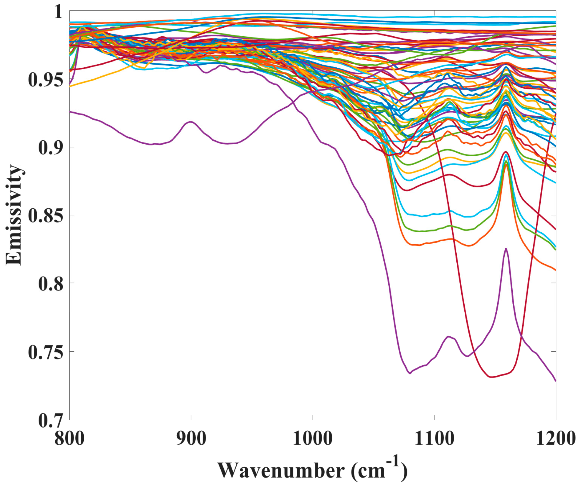
2.4. Field-Measured Data

In addition to the simulated data, field-measured data were also used to evaluate our proposed method. The field-measured data were obtained from a field campaign that occurred over three weeks in June 2004 at the ONERA (Office National d’Etudes et de Recherches Aérospatiales) center of Fauga-Mauzac [42].
This experiment measured 11 samples of a variety of surface types such as soil, stone, wood, sand, and even man-made materials. The LSEs of each sample were measured a minimum of 10 times in the laboratory by a BRUCKER-EQUINOX spectrometer equipped with an integrating sphere. The spectral radiances (from 700 to 3000 cm−1) were measured outdoors by a BOMEM (MR 250 Series) Fourier transform interferometer with a spectral resolution of 4 cm−1 and a sampling rate of 2 cm−1. The spectroradiometer was held at 1.2 m above the ground and pointed at a horizontal surface via a 45° gold mirror. The total path length from the surface to the sensor was about two meters and a 20 cm diameter footprint was provided by an AMY08 lens. In addition, a labsphere infragold plate was systematically measured before each sample to estimate the environmental downwelling radiance. The temperature of the infragold plate was recorded by a thermocouple, and the LSEs of the plate were measured in the laboratory. Because of the high values of the infragold reflectance, the self-emission term of the plate was very small. Therefore, a large uncertainty in the infragold plate’s temperature could be tolerated when estimating the environment downwelling radiance.
To obtain the real LSTs of the samples, the KT19, a broadband longwave infrared (LWIR) radiometer with a channel range of 9.5–11.5 µm and an overall estimate of uncertainty in 0.5 K, was used to record the surface leaving radiance and then used to estimate the LST by correcting for the effects of LSE and environmental downwelling radiance. The LWIR Radiometer was calibrated on a M345 MIKRON black body and the overall radiance difference between the simulated radiances and the reference radiometer measurements was less than 1%, indicating that the radiometric quality of the interferometer calibration process was high.
However, some obvious differences between the measurements of LSEs were found for certain samples in [42]. To ensure the reliability of the results, nine samples were finally selected. The details of these are listed in Table 2.

2.5. Algorithms for Evaluation

To mathematically evaluate the retrievals, this study adopted the root mean square error (RMSE) and bias. The calculations of these parameters for the LST and LSE are as follows:
R M S E T = i = 1 N S ( T i , e s t T i . a c t ) 2 N S B I A S T = i = 1 N S ( T i , e s t T i , a c t ) N S
R M S E ε = i = 1 N S j = 1 N W ( ε i , j , e s t ε i , j , a c t ) 2 N S N W B I A S ε = i = 1 N S j = 1 N W ( ε i , j , e s t ε i , j , a c t ) N S N W
where Ti,est and Ti,act are the estimated and actual LST for sample i, respectively; NS is the total number of samples during the simulation; NW is the number of wavenumbers in the selected spectral domain; and εi,j,est and εi,j,act are the estimated and actual LSE for sample i at wavenumber j, respectively.
Similar to the method described in Kanani et al. [27] for evaluating the retrievals from field-measured data, the formulas used in this paper are as follows:
σ T = 1 N M 1 i = 1 N M ( ( T i , e s t T i , a c t ) Δ T M ) 2 Δ T M = 1 N M i = 1 N M ( T i , e s t T i , a c t )
σ ε = 1 N M N W 1 i = 1 N M j = 1 N W ( ( ε i , j , e s t ε i , j , a c t ) Δ ε i , j , M ) 2 Δ ε i , j , M = 1 N M N W i = 1 N M j = 1 N W ( ε i , j , e s t ε i , j , a c t )
Δ ε max = max ( ε i , j , e s t ε i , j , a c t ) Δ ε min = min ( ε i , j , e s t ε i , j , a c t )
where NM is the number of measurements for a certain sample, NW is the number of wavenumbers in the selected TIR range, σT is the standard deviation of the difference between the estimated and actual LST, σε is the standard deviation of the difference between the estimated and actual LSEs, and Δεmax and Δεmin are the maximum and minimum of LSE channel differences, respectively.

3. Results and Discussion

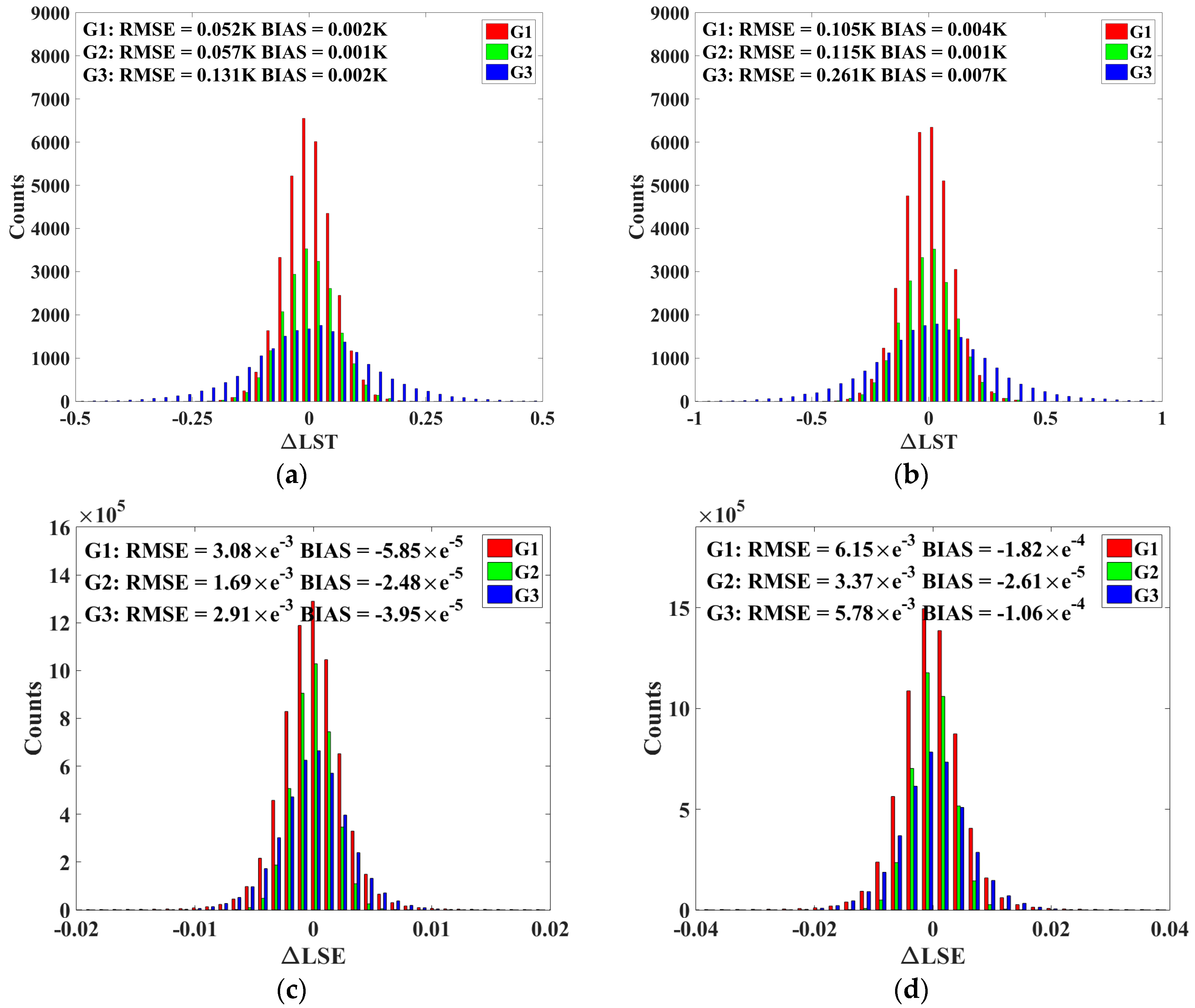
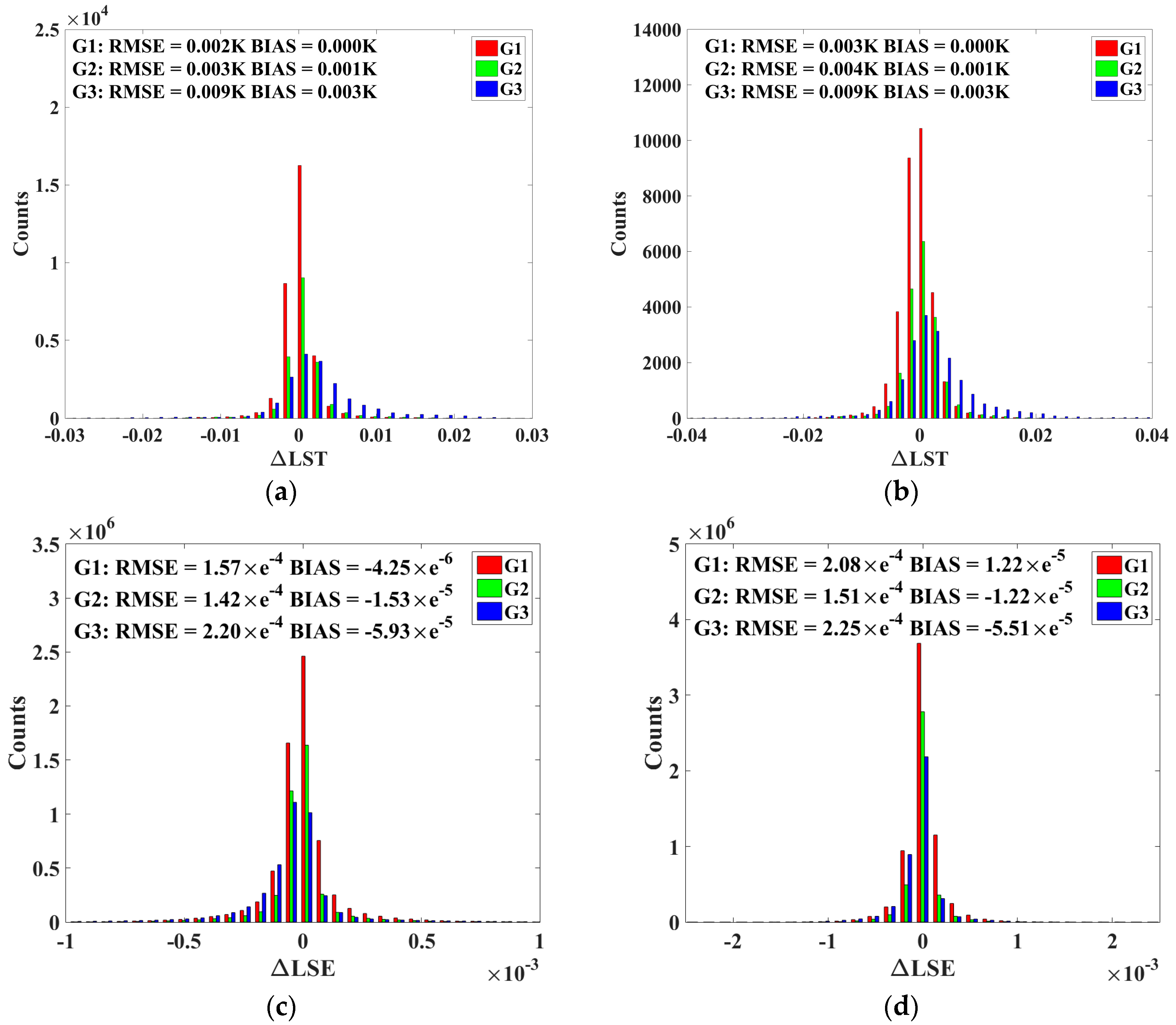
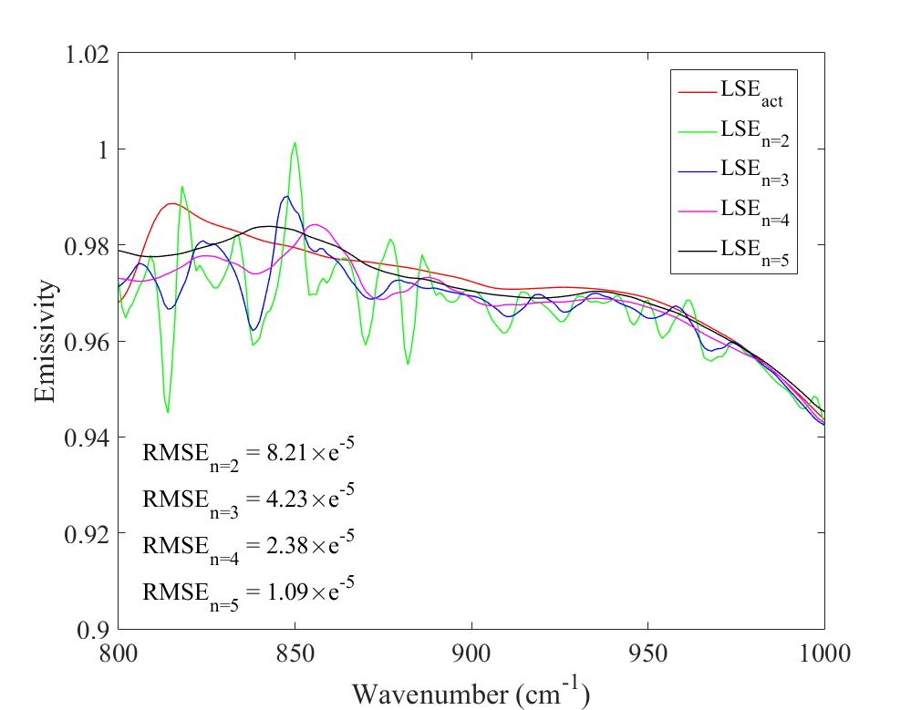
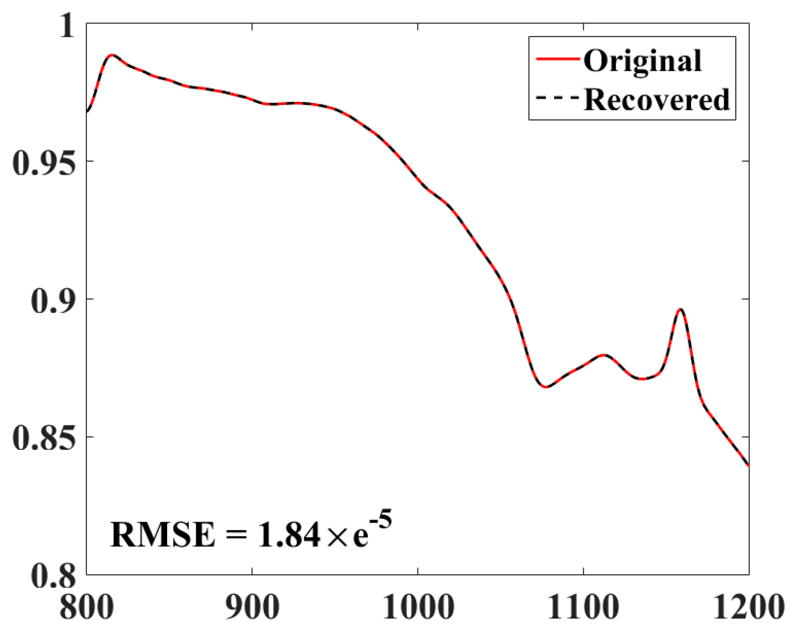
3.1. Errors introduced by the Wavelet Transform (WT)

In essence, our method simply decomposes the LSE spectrum into different frequency parts, the high- and low-frequency wavelet coefficients, and then recovers the LSEs from the low-frequency part. Because it requires no extra assumptions or prior knowledge, the only error that might be introduced is from abandoning the high-frequency part. Here, Figure 2 shows a simple example, comparing the original and recovered LSE spectrum. The sample material is one of the soils selected from the ASTER Spectral Library.
Figure 2 shows that the differences between the original and recovered LSEs are quite slight; the RMSE is only approximately 1.84 × e−5. Similar conclusions were found for various land surface materials, indicating that wavelet transform is a feasible method to reduce the unknowns in the RTE.
To better evaluate the performance of the proposed method under different atmospheric conditions, the six standard profiles were sorted into three sub-groups according to their bottom atmospheric temperatures. Group-1 (G1) consists of the Tropical and Mid-Latitude Summer Profiles, which have a relatively higher Tbottom. Group-2 (G2) consists of the 1976 US Standard and Sub-Arctic Summer Profiles, which have a moderate Tbottom. Group-3 (G3) includes the Mid-Latitude Winter and Sub-Arctic Winter Profiles, which have the lowest Tbottom.
Figure 3 shows the detailed results of the retrieved LSTs and LSEs from our proposed method under the no-error condition. The abscissas in Figure 3a,b denote the errors of the LSTs and LSEs, respectively. The different colors in Figure 3 indicate the different sub-groups. Note that because the overall accuracy improves slightly by using a higher wavelet level, more time is consumed, and a wavelet level of n = 2 is actually used in this paper, unless otherwise specified.
The results in Figure 3 show that the overall difference between the original and recovered LSEs is quite small; the RMSEs are only 1.38 × e−4 for G1, 1.40 × e−4 for G2, and 2.18 × e−4 for G3, and the maximum error is below 0.1%. For LST retrievals, the corresponding RMSEs are 0.002 K for G1, 0.003 K for G2, and 0.009 K for G3. Clearly, the accuracy of G3 is lower than that of the others; however, the value of RMSE is still quite small and can be ignored. From Figure 3, all the bias values are shown to be close to zero, which indicates that our method can give a no-bias estimate of the LSTs and LSEs under a no-error condition.
The results in Figure 3 confirm that the LSEs can be better recovered from the low-frequency wavelet coefficients by using the wavelet transform. However, due to the features of the wavelet transform, this approach is more suitable for hyperspectral data.

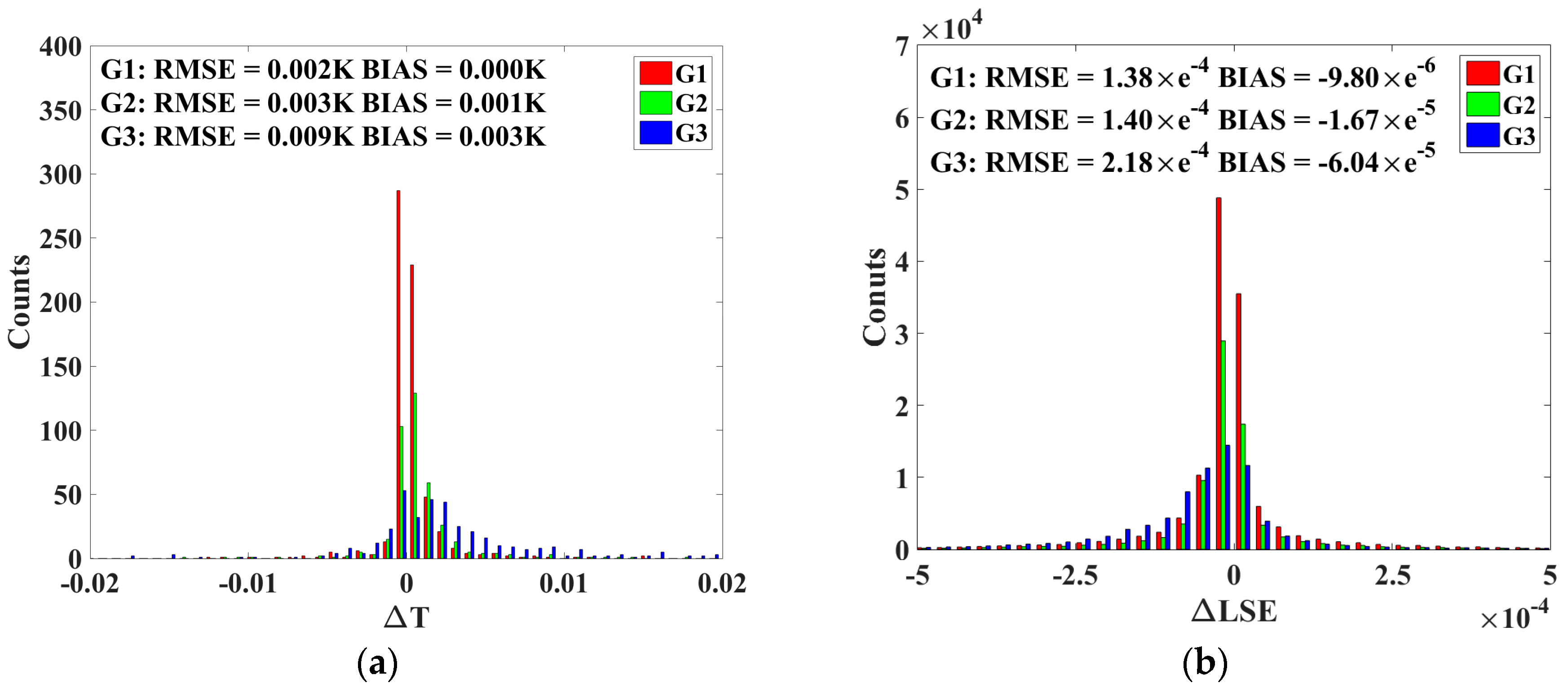
3.2. Sensitivity to Instrument Noise

In this section, instrument noise is considered to further evaluate the performance of the WTTES algorithm. To improve the accuracy evaluation, two different levels of error (0.1, 0.2 K) in the form of NE∆T were finally used, and all errors were added to the at-ground radiance. Note that all the errors in this paper are considered with no bias.
Figure 4 shows histograms of the LST and LSE errors with different levels of instrument noise: NE∆T = 0.1 K and NE∆T = 0.2 K. The abscissa denotes the errors in the LSTs and LSEs, and the ordinate denotes the number of elements.
According to Figure 4, when NE∆T = 0.1 K, the RMSEs of the retrieved LSTs in each sub-group are 0.052, 0.057, and 0.131 K, respectively, with almost no bias. When NE∆T = 0.2 K, they are 0.105, 0.115, and 0.261 K, respectively, with almost no bias. It is quite clear that the retrieval accuracy from G3 is slightly lower than that from G1 and G2, which agrees with the conclusions in Section 3.1. This result occurs because the water vapor contents of the profiles in G3 are the lowest of the six selected profiles. Because water vapor is the main absorbent in the TIR range, the atmospheric features of the LSE spectrum will be weakened, making it difficult to find the optimal LSTs and LSEs through the iterative process, especially under conditions with errors. Even so, the overall accuracy of G3 for LST is still below 0.3 K when NE∆T = 0.2 K. Compared with the LST, our method always achieves a better accuracy for the LSEs, all of which are below 1% with different levels of errors. Furthermore, all the LSEs are still estimated in an un-biased fashion, which demonstrates the high anti-noise properties of our method.
One reason for the high anti-noise robustness of our algorithm is because of the use of the least-squares technique in solving the nonlinear RTE, which has been shown to be effective in reducing such white noise. The other reason is because the added instrument noise is contained in the retrieved spectral emissivity, and this error can be further reduced through the use of WT.

3.3. Sensitivity to the Atmospheric Downwelling Radiance

In addition to instrument noise, varying error levels of atmospheric downwelling radiance are considered in this section to evaluate our proposed method. To directly compare the performance with instrument errors, the same approach for adding errors is used here. The final results are shown in Figure 5.
Compared with the errors of at-ground radiance, our method is obviously insensitive to the uncertainty of atmospheric downwelling radiance. For both levels of error, the RMSEs of the estimated LST range from 0.002 to 0.009 K, with almost no bias. The accuracy of the un-biased LSEs is between 1.42 × e−4 and 2.25 × e−4. Similar to the previous results, the overall accuracy of the retrievals from G3 is still lower than the others. However, no obvious influence on the accuracy of the estimated LSTs and LSEs can be found by increasing the NE∆T from 0.1 to 0.2 K. In other words, in most cases, it is reasonable to ignore the errors caused by the uncertainty of the atmospheric downwelling radiance for most typical surfaces. The possible reasons for the low sensitivity of the WTTES algorithm to the atmospheric downweling may be either that: (1) most selected materials have an LSE of larger than 0.9, which makes the contribution of the atmospheric downwelling radiance small compared with that of the surface-emitted radiance; or that (2) only white noise from atmospheric downwelling radiance is considered in this paper, which can be removed more efficiently by using the least-squares technique.

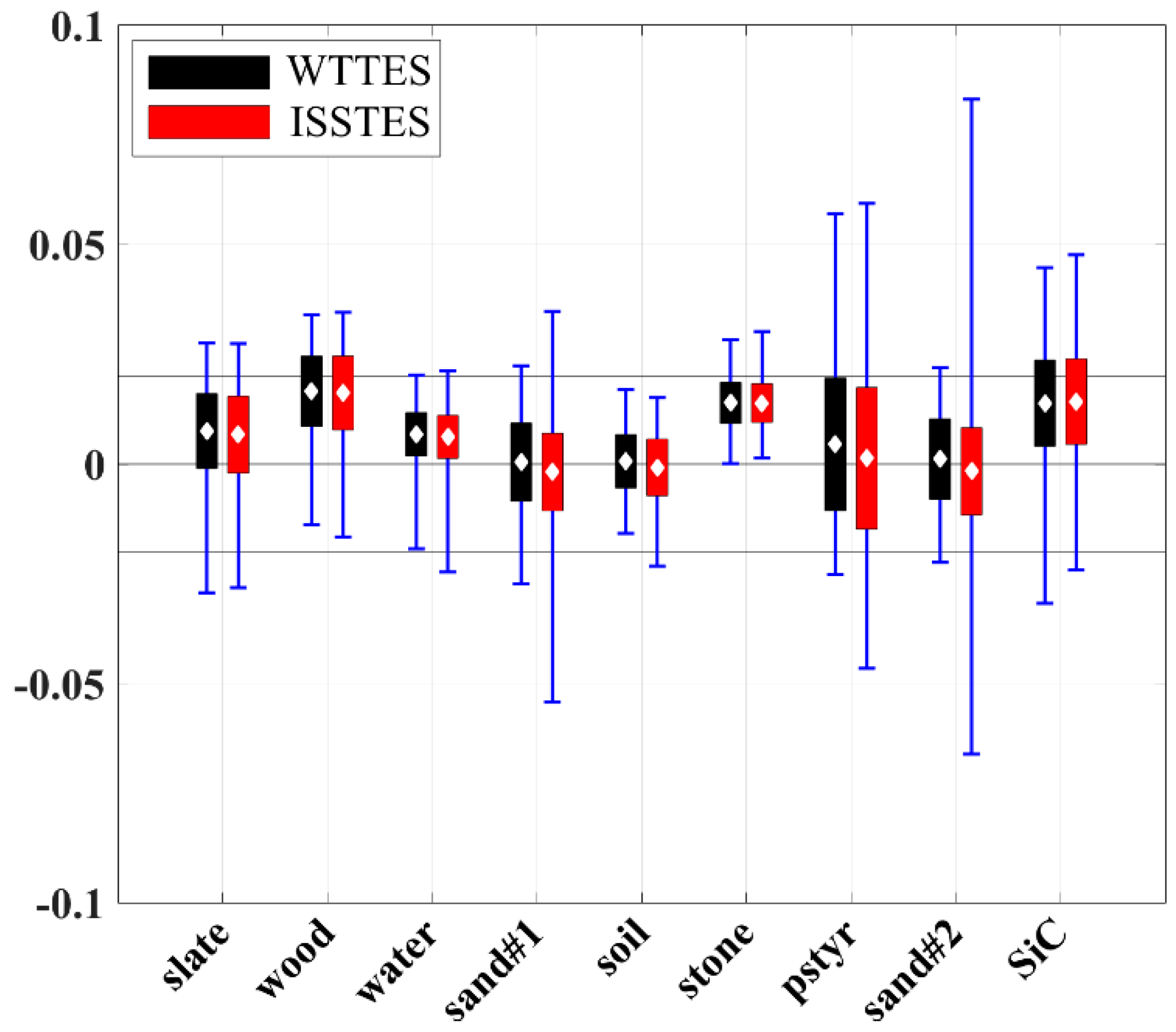
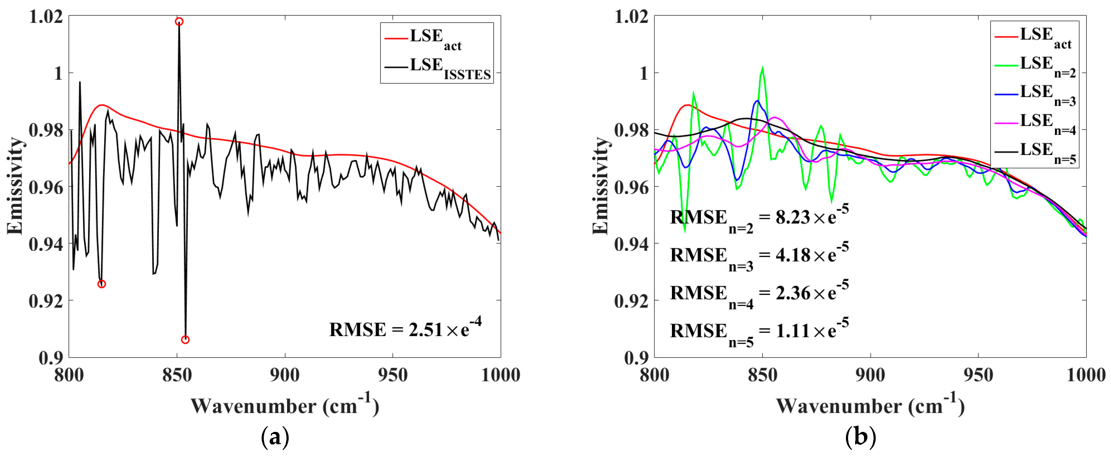
3.4. Comparison of the WTTES Algorithm with the ISSTES Algorithm

Currently, the ISSTES algorithm is the most widely used algorithm for separating LSTs and LSEs from hyperspectral TIR data. Therefore, this section shows a comparison of the performance of our method and that of the ISSTES algorithm. All the results in this section are obtained from the same data used in the previous sections. Additionally, a higher level of noise (NE∆T = 0.5 K) is also adopted in this section for further analysis and comparison. The final results are given in Table 3.
From the results in Table 3, our method clearly achieves an accuracy comparable to the ISSTES algorithm. In most cases, the differences between these two algorithms are below approximately 0.05 K for LSTs and 0.1% for LSEs. However, our method achieves slightly better results than the ISSTES algorithm when the error increases. When NE∆T = 0.1 K, the maximum difference for the LST is only approximately 0.03 K; however, it becomes approximately 0.1–0.2 K when the NE∆T increases to 0.5 K. Moreover, as noted above, both algorithms are suitable for a wet-warm profile
In fact, the present ISSTES method can only ensure the overall accuracy of the LSEs. There are usually numerous peaks and valleys, and even some obvious singular points, in the retrieved LSE spectrum when obvious instrument noise is present. A simple example is shown in Figure 6a.
The LSEs retrieved by ISSTES have an RMSE of only 2.51×e-4; however, their spectral shapes fluctuate wildly and some obvious singular points, encircled with red, can also be found. To overcome this problem, our proposed method introduces the parameter n to determine the wavelet transform levels.
Based on Formulas (3) and (4), one can change the value of n according to a specific requirement along with the noise level. To put it simply, if one needs the details of LSE spectral information or no obvious instrument noise is found, a value of n = 2 is recommended (this value was the number used in the previous sections). If the overall shape of the LSE spectrum is needed or obvious noise is present, then a higher number of n is expected.
From the results in Figure 6b, the obvious conclusion is that our method is better at removing the singular points from the LSE spectrum through the selection of a suitable n. In addition, the LSE spectrum obtained with our method is quite smooth compared to that of ISSTES and no obvious RMSE of LSEs is found. However, because only a simple test is performed in this section, the performance of our method with different levels (n) has not been fully evaluated. A known limitation is that, for a fluctuating LSE spectrum, a level of n = 5 in this paper will lose some spectral features in certain channels, such as the retrieved LSEs in the range of 800–850 cm−1 in Figure 6b. Nevertheless, because most of the land surface materials have a smooth spectrum in the 800–1000 cm−1 range, the effect of using a larger number of n might be decreased to some extent.

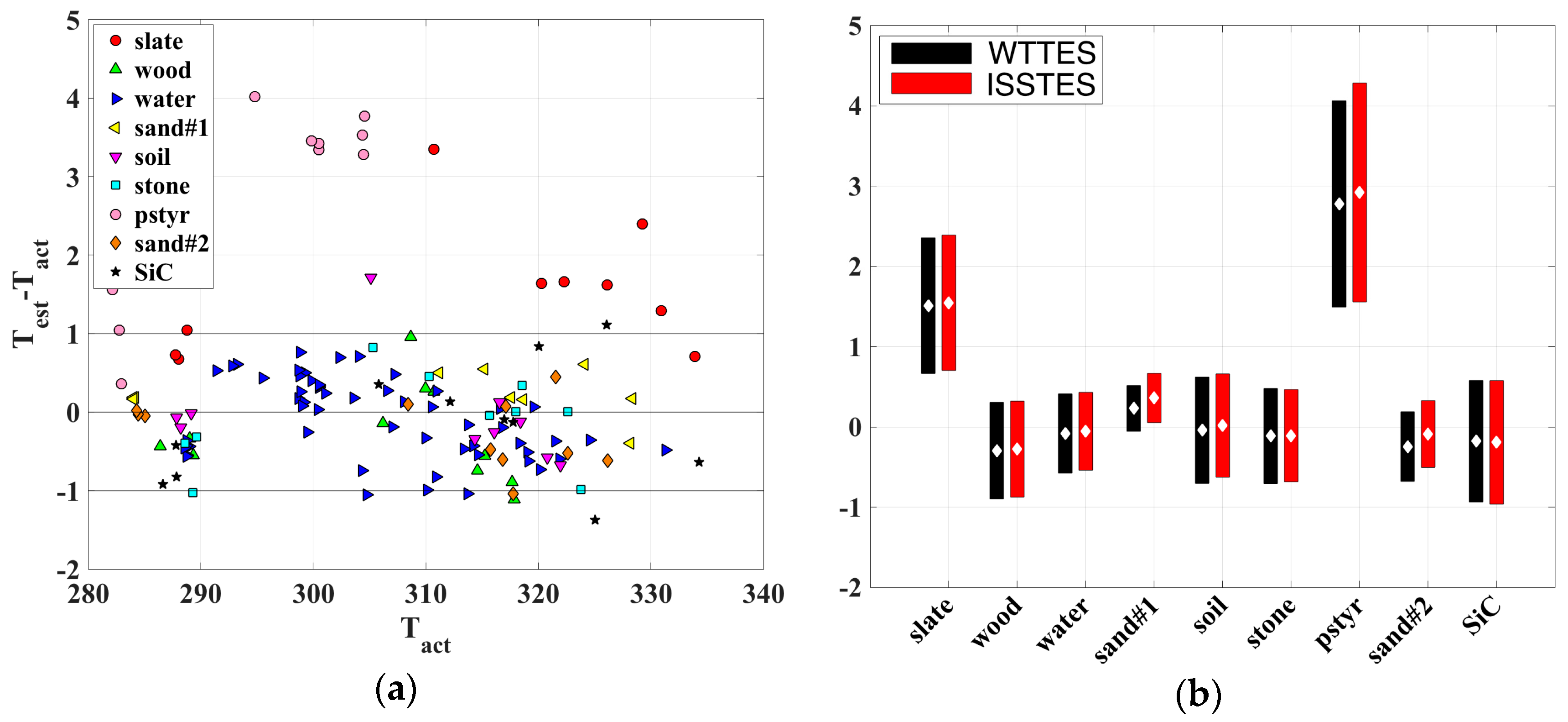
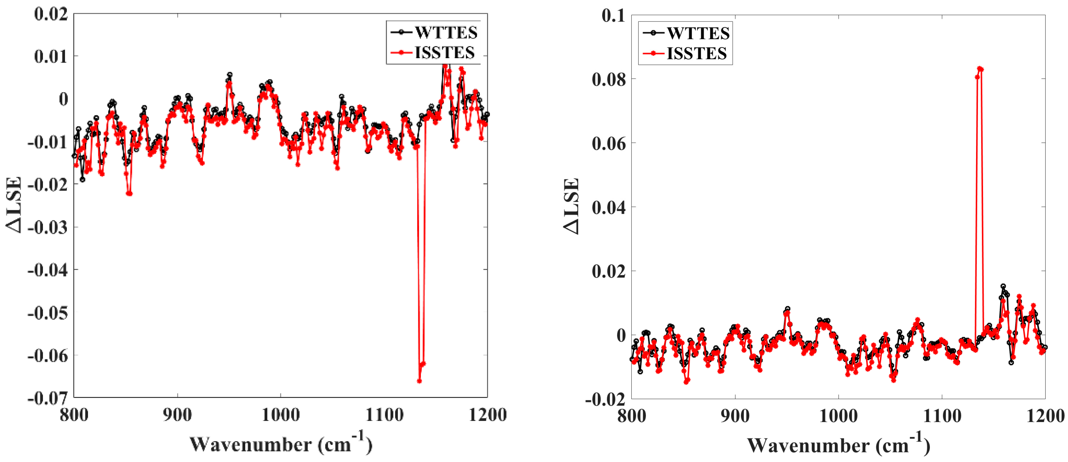
3.5. Evaluation with Field-Measured Data

In this section, field-measured data are used to evaluate our proposed method, including a comparison with the ISSTES algorithm. It should be noted that, for each sample, the averages of all LSEs measured in the laboratory are taken as the actual LSEs. The LST results from the WTTES and ISSTES algorithms are shown in Figure 7.
Consistent with the previous conclusions from simulated data, no obvious difference could be found between these two algorithms (Figure 7). According to the actual LSTs, 114 of 138 measurements have an LST difference of less than 1 K from the WTTES algorithm, while 117 measurements show the same accuracy as that from the ISSTES algorithm. The results indicate that both these algorithms provide relatively accurate LST retrievals from field-measured data. However, for some special materials, the LST differences are much larger, especially for the manmade material of pstyr. Most of the LST errors for pstyr are larger than 3 K.
Figure 8 gives the results of the estimated LSEs from both algorithms.
According to the retrievals, the RMSEs of the estimated LSEs could be within 1% for the samples of slate, water, sand#1, soil, and sand#2, whereas, for the samples of wood, stone, pstyr, and SiC, the RMSEs increase to approximately 1.5%–1.9%. These larger RMSEs for both the LST and LSE may be caused by the different IFOVs of instruments, the different sample locations, or the uncertainty of each measurement.
However, similar to the LST results, the overall accuracy of the LSEs retrieved by these two algorithms is quite consistent. The ISSTES algorithm will still lead to some singular channel LSEs when considering the performance at each channel, especially for the sand#2 sample used in this paper. The maximum value of the differences in the channel LSEs is approximately 0.08.
To clearly demonstrate the singular problem, the sample of sand#2 was chosen to show the error spectrum. In total, there were 11 measurements of sand#2, measured 11 times in one day. While there was little difference between nine of the measurements, two were found with singular points because of the measurement circumstances, as shown in Figure 9.
From Figure 9, some larger differences can clearly be found in the 1130–1140 cm−1 range when using the ISSTES algorithm. This phenomenon may occur when the surface-emitted radiance Bi(Ts) is close to the environmental downwelling radiance Li,down. Similar results were found for the sand#1 and pstyr samples used in this paper. However, it should be noted that the singular points problem in the ISSTES algorithm has nothing to do with the type of surface. Instead, it is caused primarily by the measurement conditions.

4. Conclusions

This paper proposed a WTTES algorithm that can accurately and effectively separate the LSTs and LSEs from field-measured hyperspectral TIR data. By decomposing the LSEs and then reconstructing them from the low-frequency wavelet coefficients, the process of temperature and emissivity separation has been changed to one of calculating the temperature and low-frequency wavelet coefficients, a procedure that obviously reduces the unknowns in the RTE. No prior knowledge or assumptions are necessary in our method, making it much more efficient. Moreover, because the spectral emissivity is directly recovered from the low-frequency wavelet coefficients instead of the simple inversion of the RTE, both the singular problem and the discontinuity problem can be solved effectively.
To evaluate the performance of our method, different kinds and levels of error were considered in this paper. Examples include errors of instrument noise and atmospheric downwelling radiance in the form of NE∆T (0.1 and 0.2 K). The results show that the errors introduced by the WT are negligible. The overall accuracy of our method, with no errors, is between 0.002 and 0.009 K for LSTs and between 1.38 × e−4 and 2.18 × e−4 for LSEs. When instrument noise exists, the accuracy will be decreased somewhat. However, compared with the instrument noise, errors from atmospheric downwelling radiance are sufficiently small that no obvious change can be found in the RMSEs for either the LSTs or LSEs. In other words, our method is quite insensitive to the uncertainty of atmospheric downwelling radiance for typical surfaces such as soil, vegetation, and water. Additionally, the results also indicate that the performance of our method is usually better under wet-warm atmospheric conditions than under a dry-cold atmospheric profile. Compared to the current ISSTES algorithm, our method not only obtains comparable accuracy in most cases, but also eliminates singular points. Furthermore, a multi-level solution is also available in our method to adapt it to different requirements, without losing the overall accuracy. For field measurements, the overall RMSEs of the retrieved LSTs and LSEs are approximately 1.1 K and 1%, respectively. No obvious differences were found between the WTTES and ISSTES algorithms, which might have been be caused by the high signal-to-noise ratio (SNR) in the measured data. However, while some obvious singular channel LSEs can still be found in the ISSTES retrievals, our proposed method removes them.
This investigation of the WTTES algorithm for field-measured TIR data is encouraging. We plan to perform extensive tests in the near future to investigate the performance of the WTTES algorithm for airborne and satellite data.

Acknowledgments

This study was supported by National Key Basic Research Program of China (973 Program, 2013CB733402); National Natural Science Foundation of China (41331171, 41571352 and 41471297); Innovation Project of LREIS (O88RA801YA).

Author Contributions

Yu-Ze Zhang, Hua Wu, and Xiao-Guang Jiang conceived this work, conducted the analyses, and wrote the paper; Ya-Zhen Jiang contributed to the data processing; Zhao-Xia Liu provided theoretical guidance for this work and the paper; Franҫoise Nerry provided the field-measured data and supervision of the methods employed; All authors helped in the editing and revision of the manuscript.

Conflicts of Interest

The authors declare no conflict of interest.

References

  1. Dash, P.; Olesen, F.S.; Fischer, H. Land surface temperature and emissivity estimation from passive sensor data: Theory and practice-current trends. Int. J. Remote Sens. 2002, 23, 2563–2594. [Google Scholar] [CrossRef]
  2. Li, Z.L.; Wu, H.; Wang, N.; Shi, Q.; Sobrino, J.A.; Wan, Z.; Tang, B.H.; Yan, G. Land surface emissivity retrieval from satellite data. Int. J. Remote Sens. 2013, 34, 3084–3127. [Google Scholar] [CrossRef]
  3. Li, Z.L.; Tang, B.H.; Wu, H.; Ren, H.Z.; Yan, G.J.; Wan, Z.M.; Trigo, I.F.; Sobrino, J.A. Satellite-derived land surface temperature: Current status and perspectives. Remote Sens. Environ. 2013, 131, 14–37. [Google Scholar] [CrossRef]
  4. Quattrochi, D.A.; Goel, N.S. Spatial and temporal scaling of thermal infrared remote sensing data. Remote Sens. Rev. 1995, 12, 255–286. [Google Scholar] [CrossRef]
  5. Hook, S.J.; Gabell, A.R.; Green, A.A.; Kealy, P.S. A comparison of techniques for extracting emissivity information from thermal infrared data for geologic studies. Remote Sens. Environ. 1992, 42, 123–135. [Google Scholar] [CrossRef]
  6. Hook, S.J.; Karlstrom, K.E.; Miller, C.F.; McCaffrey, K.J.W. Mapping the Piute Mountains, California, with thermal infrared multi- spectral scanner (TIMS) images. J. Geophys. Res. 1994, 99, 15605–15622. [Google Scholar] [CrossRef]
  7. Salisbury, J.W.; D’Aria, D.M. Emissivity of terrestrial materials in the 8–14 μm atmospheric window. Remote Sens. Environ. 1992, 42, 83–106. [Google Scholar] [CrossRef]
  8. Realmuto, V.J. Separating the effects of temperature and emissivity: Emissivity spectrum normalization. In Proceedings of the 2nd TIMS Workshop, Pasadena, CA, USA, 6 June 1990. [Google Scholar]
  9. Wan, Z.; Dozier, J. A generalized split-window algorithm for retrieving land-surface temperature from space. IEEE Trans. Geosci. Remote Sens. 1996, 34, 892–905. [Google Scholar]
  10. Wan, Z.; Li, Z.L. A physics-based algorithm for retrieving land-surface emissivity and temperature from EOS/MODIS data. IEEE Trans. Geosci. Remote Sens. 1997, 35, 980–996. [Google Scholar]
  11. Gillespie, A.; Rokugawa, S.; Matsunaga, T.; Cothern, J.S.; Hook, S.; Kahle, A.B. A temperature and emissivity separation algorithm for Advanced Spaceborne Thermal Emission and Reflection Radiometer (ASTER) images. IEEE Trans. Geosci. Remote Sens. 1998, 36, 1113–1126. [Google Scholar] [CrossRef]
  12. Kahle, A.B.; Madura, D.P.; Soha, J.M. Middle infrared multispectral aircraft scanner data: analysis for geological applications. Appl. Opt. 1980, 19, 2279–2290. [Google Scholar] [CrossRef] [PubMed]
  13. Barducci, A.; Pippi, I. Temperature and emissivity retrieval from remotely sensed images using the “Grey body emissivity” method. IEEE Trans. Geosci. Remote Sens. 1996, 34, 681–695. [Google Scholar] [CrossRef]
  14. Gillespie, A.R. Lithologic mapping of silicate rocks using TIMS (Thermal Infrared Multispectral Scanner). In Proceedings of the Thermal Infrared Multispectral Scanner Data User’s Workshop, Pasadena, CA, USA, 18–19 June 1985. [Google Scholar]
  15. Mao, K.; Shi, J.; Tang, H.; Li, Z.L.; Wang, X.; Chen, K.S. A neural network technique for separating land surface emissivity and temperature from ASTER imagery. IEEE Trans. Geosci. Remote Sens. 2008, 46, 200–208. [Google Scholar] [CrossRef]
  16. Li, Z.L.; Becker, F.; Stoll, M.P.; Wan, Z. Evaluation of Six Methods for Extracting Relative Emissivity Spectra from Thermal Infrared Images. Remote Sens. Environ. 1999, 69, 197–214. [Google Scholar] [CrossRef]
  17. Aumann, H.H.; Chahine, M.T.; Gautier, C.; Goldberg, M.D.; Kalnay, E.; McMillin, L.M.; Revercomb, H.; Rosenkranz, P.W.; Smith, W.L.; Staelin, D.H.; et al. AIRS/AMSU/HSB on the Aqua mission: Design, science objectives, data products, and processing systems. IEEE Trans. Geosci. Remote Sens. 2003, 41, 253–264. [Google Scholar] [CrossRef]
  18. Chalon, G.; Cayla, F.; Diebel, D. IASI-An advanced sounder for operational meteorology. In Proceedings of the 52nd IAF, International Astronautical Congress, Toulouse, France, 1–5 October 2001. [Google Scholar]
  19. Siméoni, D.; Singer, C.; Chalon, G. Infrared atmospheric sounding interferometer. Acta Astronaut. 1997, 40, 113–118. [Google Scholar] [CrossRef]
  20. Glumb, R.J.; Mantica, P. Development of the Crosstrack Infrared Sounder (CrIS) sensor design. Proc. SPIE Int. Soci. Opt. Eng. 2002, 4486, 411–424. [Google Scholar]
  21. Borel, C.C. Surface emissivity and temperature retrieval for a hyperspectral sensor. In Proceedings of the 1998 IEEE International Geoscience and Remote Sensing Symposium (IGARSS), Seattle, WA, USA, 6–10 July 1998; pp. 546–549. [Google Scholar]
  22. Wang, N.; Wu, H.; Nerry, F.; Li, C.; Li, Z.L. Temperature and emissivity retrievals from hyperspectral thermal infrared data using linear spectral emissivity constraint. IEEE Trans. Geosci. Remote Sens. 2011, 49, 1291–1303. [Google Scholar] [CrossRef]
  23. Wang, X.; Ouyang, X.; Tang, B.; Li, Z.L.; Zhang, R. A New Method for Temperature/Emissivity Separation from Hyperspectral Thermal Infrared Data. In Proceedings of the 2008 IEEE International Geoscience and Remote Sensing Symposium (IGARSS), Boston, MA, USA, 8–11 July 2008. [Google Scholar]
  24. Cheng, J.; Liang, S.; Wang, J.; Li, X. A Stepwise Refining Algorithm of Temperature and Emissivity Separation for Hyperspectral Thermal Infrared Data. IEEE Trans. Geosci. Remote Sens. 2010, 48, 1588–1597. [Google Scholar] [CrossRef]
  25. Adler-golden, S.; Conforti, P.; Gagnon, M.; Tremblay, P.; Chamberland, M. Long-wave infrared surface reflectance spectra retrieved from Telops Hyper-Cam imagery. In Proceedings of the SPIE-The International Society for Optical Engineering, Baltimore, MD, USA, 5 May 2014; pp. 90880U:1–90880U:8. [Google Scholar]
  26. Wu, H.; Li, Z.L.; Tang, B.H.; Tang, B.L. Evaluation of the improved linear emissivity constraint temperature and emissivity separation method by using the simulated hyperspectral thermal infrared data. In Proceedings of the 2015 SPIE 9808, International Conference on Intelligent Earth Observing and Applications, Guilin, China, 23 October 2015. 98082L. [Google Scholar]
  27. Wu, H.; Wang, N.; Ni, L.; Tang, B.H.; Li, Z.L. Practical retrieval of land surface emissivity spectra in 8–14 μm from hyperspectral thermal infrared data. Opt. Express 2012, 20, 24761–24768. [Google Scholar] [CrossRef] [PubMed]
  28. Zhou, L.; Goldberg, M.; Barnet, C.; Cheng, Z.; Sun, F.; Wolf, W.; Divakarla, M. Regression of Surface Spectral Emissivity from Hyperspectral Instruments. IEEE Trans. Geosci. Remote Sens. 2008, 46, 328–333. [Google Scholar] [CrossRef]
  29. Berk, A.; Anderson, G.P.; Bernstein, L.S.; Acharya, P.K.; Dothe, H.; Matthew, M.W.; Adler-Golden, S.M.; Chetwynd, J.H.; Richtsmeier, S.C.; Pukall, B.; et al. MODTRAN4 radiative transfer modeling for atmospheric correction. Proc. SPIE Int. Soc. Opt. Eng. 1999, 3756, 348–353. [Google Scholar]
  30. Gu, D.; Gillespie, A.R.; Kahle, A.B.; Palluconi, F.D. Autonomous Atmospheric Compensation (AAC) of high-resolution hyperspectral thermal infrared remote-sensing imagery. IEEE Trans. Geosci. Remote Sens. 2000, 38, 2557–2570. [Google Scholar]
  31. Young, S.J.; Johnson, B.R.; Hackwell, J.A. An in-scene method for atmospheric compensation of thermal hyperspectral data. J. Geophys. Res. Atmos. 2002, 107, ACH 14-1–ACH 14-20. [Google Scholar] [CrossRef]
  32. Tonooka, H. An atmospheric correction algorithm for thermal infrared multispectral data over land-a water-vapor scaling method. IEEE Trans. Geosci. Remote Sens. 2001, 39, 682–692. [Google Scholar] [CrossRef]
  33. Tonooka, H.; Palluconi, F.D. Validation of ASTER/TIR Standard Atmospheric Correction Using Water Surfaces. IEEE Trans. Geosci. Remote Sens. 2005, 43, 2769–2777. [Google Scholar] [CrossRef]
  34. Tonooka, H. Accurate atmospheric correction of ASTER thermal infrared imagery using the WVS method. IEEE Trans. Geosci. Remote Sens. 2005, 43, 2778–2792. [Google Scholar] [CrossRef]
  35. Farge, M. Wavelet Transforms and their Applications to Turbulence. Annu. Rev. Fluid. Mech. 1992, 24, 395–457. [Google Scholar] [CrossRef]
  36. Daubechies, I. The wavelet transform, time-frequency localization and signal analysis. IEEE Trans. Inf. Theory 1990, 36, 961–1005. [Google Scholar] [CrossRef]
  37. Daubechies, I. Ten Lectures on Wavelets; Society for Industrial and Applied Mathematics: Philadelphia, PA, USA, 1992. [Google Scholar]
  38. Borel, C. Error analysis for a temperature and emissivity retrieval algorithm for hyperspectral imaging data. Int. J. Remote Sens. 2008, 29, 5029–5045. [Google Scholar] [CrossRef]
  39. Berk, A.; Anderson, G.P.; Acharya, P.K.; Bernstein, L.S.; Matthew, M.W.; Golden, S.M. MODTRAN4 User’s Manual; Air Force Research Laboratory, Space Vehicles Directorate: HANSCOM AFB, MA, USA, 1999. [Google Scholar]
  40. Baldridge, A.M.; Hook, S.J.; Grove, C.I.; Rivera, G. The ASTER spectral library version 2.0. Remote Sens. Environ. 2009, 113, 711–715. [Google Scholar] [CrossRef]
  41. Tang, B.H.; Bi, Y.Y.; Li, Z.L.; Xia, J. Generalized Split-Window Algorithm for Estimate of Land Surface Temperature from Chinese Geostationary FengYun Meteorological Satellite (FY-2C) Data. Sensors 2008, 8, 933–951. [Google Scholar] [CrossRef] [PubMed]
  42. Kanani, K.; Poutier, L.; Nerry, F.; Stoll, M.P. Directional effects consideration to improve out-doors emissivity retrieval in the 3–13 µm domain. Opt. Express 2007, 15, 12464–12482. [Google Scholar] [CrossRef] [PubMed]
Figure 1. All 65 LSE spectra from the ASTER spectral Library. The abscissa is the wavenumber in cm−1, and the ordinate shows the LSE values.
Remotesensing 09 00454 g001
Figure 2. Comparison of the original LSE spectrum and the recovered LSE spectrum from wavelet transform. The abscissa is the wavenumber in cm−1, and the ordinate is the LSEs. The sample material is one of the soils selected from the ASTER Spectral Library.
Remotesensing 09 00454 g002
Figure 3. Details of the errors introduced by the WT method for 65 LSEs under the six standard profiles. The abscissas in (a) and (b) denote the LST and LSE errors, respectively, and the ordinate shows the numbers of elements for (a) LST and (b) LSE.
Remotesensing 09 00454 g003
Figure 4. Histograms of LST and LSE errors caused by different levels of instrument noise. The abscissa denotes the LST and LSE errors, and the ordinate denotes the numbers of elements. (a) NE∆T = 0.1 K for LST; (b) NE∆T = 0.2 K for LST; (c) NE∆T = 0.1 K for LSE; (d) NE∆T = 0.2 K for LSE.
Remotesensing 09 00454 g004
Figure 5. Histograms of LST and LSE errors caused by the uncertainty of atmospheric downwelling radiance. The abscissa denotes the LST and LSE errors, and the ordinate denotes the numbers of elements: (a) NE∆T = 0.1 K for LST; (b) NE∆T = 0.2 K for LST; (c) NE∆T = 0.1 K for LSE; (d) NE∆T = 0.2 K for LSE.
Remotesensing 09 00454 g005
Figure 6. Plots of the retrieved LSE spectra with an error of NE∆T = 0.2 K for Li,g from the (a) ISSTES algorithm and (b) WTTES algorithm. The different colors indicate the results with different wavelet transform levels: n = 2, 3, 4, and 5.
Remotesensing 09 00454 g006
Figure 7. (a) Differences between the estimated and actual LST from the field-measured data with the WTTES algorithm. The abscissa is the actual LST (Tact), and the ordinate is the difference between the estimated LST (Test) and the actual LST; (b) Comparison of the LST errors with the WTTES and ISSTES algorithms. The center point of each bar is equal to ΔTM, and the half-length of the bar is equal to σT.
Remotesensing 09 00454 g007
Figure 8. Comparison of the estimated LSEs with the actual LSEs from the field-measured data with the WTTES algorithm and ISSTES algorithm. The bars are centered on Δεi,j,M, and the half-length of the bar is equal to σε. The endpoints of the blue line are equal to Δεmin, and Δεmax, respectively.
Remotesensing 09 00454 g008
Figure 9. Differences between the estimated and actual LSEs of the sand#2 sample (2 measurements) at each channel from 800 to 1200 cm−1 from the WTTES and ISSTES algorithms.
Remotesensing 09 00454 g009
Table 1. Details of the six profiles selected for the simulations.
ProfilesTotal Water Vapor (g/cm2)Bottom Atmospheric Temperature (K)Latitude ( ° )
1976 US Standard Atmosphere1.42288.1--
Tropical Atmosphere4.08299.715 North
Mid-Latitude Summer2.91294.245 North
Mid-Latitude Winter0.82272.245 North
Sub-Arctic Summer2.08287.260 North
Sub-Arctic Winter0.42257.260 North
Table 2. Details of the selected samples.
NameDescription
slateHomogeneous and flat piece of slate.
Composition: SiO2 (60%), Al2O3 (17%), Fe2O3 (7.6%), K2O (3.9%), MgO (2.5%), …
woodPlywood.
waterWater.
sand#1Morocco sand. Red color. Various grain sizes < 750 μm.
Composition: SiO2 (96.3%), Al2O3 (1%), ...
soilSoil from the Negev desert. Various grain sizes < 2 mm.
Composition: SiO2 (42.2%), CaO (22.8%), Al2O3 (5.5%), Fe2O3 (2.7%), ...
stone#2Flat rough and homogenous rock.
Composition: SiO2 (77%), Al2O3 (12.6%), K2O (4.6%), Na2O (3.1%), Fe2O3 (1.2%), ...
sand#2Fontainebleau type sand. Various grain sizes < 750 μm.
Composition: SiO2 (98.4%), Al2O3 (0.6%), ...
pstyrExtruded polystyrene.
SiCSiC Powder. Grain size ~ 120 μm.
Table 3. RMSEs of estimated LSTs and LSEs using the ISSTES and WTTES algorithms with different levels of error on Li,g.
GroupMethodNE∆T = 0.1 KNE∆T = 0.2 KNE∆T = 0.5 K
G1ISSTES
WTTES
0.07 K
0.05 K
0.13 K
0.10 K
0.35 K
0.29 K
RMSETG2ISSTES
WTTES
0.07 K
0.06 K
0.14 K
0.11 K
0.41 K
0.34 K
G3ISSTES
WTTES
0.16 K
0.13 K
0.31 K
0.26 K
0.85 K
0.70 K
G1ISSTES
WTTES
0.41%
0.31%
0.79%
0.62%
1.87%
1.48%
RMSEεG2ISSTES
WTTES
0.21%
0.17%
0.40%
0.34%
1.00%
0.84%
G3ISSTES
WTTES
0.35%
0.29%
0.69%
0.58%
1.79%
1.49%

