
Improving the Impervious Surface Estimation from Hyperspectral Images Using a Spectral-Spatial Feature Sparse Representation and Post-Processing Approach

School of Information Science and Engineering, Yanshan University, Qinhuangdao 066004, China
*
Authors to whom correspondence should be addressed.
Remote Sens. 2017, 9(5), 456; https://doi.org/10.3390/rs9050456
Submission received: 26 February 2017
/
Revised: 1 May 2017
/
Accepted: 4 May 2017
/
Published: 8 May 2017
Abstract
:Impervious surfaces have been widely recognized as an indicator for urbanization and environment monitoring. Plenty of methods have been proposed to extract impervious surfaces using remote sensing images. However, accurately extracting impervious surface is still a challenging task due to the confusion between impervious surface and bare soil. Thus, this paper presents a hybrid approach consisting of spectral-spatial feature sparse representation (SS-SR) and post-processing to extract urban impervious surface from hyperspectral images. We first extracted spectral and spatial features from hyperspectral images. Then, the spectral and spatial information of a pixel is represented by the vector stacking strategy. Each pixel vector can be represented by a linear combination of a few atoms from a learned dictionary, which is more suitable for impervious surface estimation. The sparse coefficients were automatically learned and then used for extracting impervious surface. The proposed impervious surface extraction method was evaluated with four hyperspectral datasets. We compared our algorithms with the state-of-the-art per-pixel based impervious surface extraction methods. The encouraging experimental results demonstrate the SS-SR algorithm generally outperforms the classic support vector machines and random forest. The improvement is more significant when combining SS-SR with post-classification approach.
1. Introduction
Impervious surfaces, such as houses, cement or asphalt roads, parking lots and other artificial surface, are defined as anthropogenic features through which water cannot infiltrate into soil [1]. Due to the impermeable feature, impervious surfaces heavily affect the urban hydrological and energy balances. Accurately extracting the extent and spatial distribution of impervious surfaces is crucial for urban heat island analysis, land use change, and climate modeling. Meanwhile, improving the impervious surface estimation is important but challenging due to the complexity of urban surface.
The remote sensing technique has become a very important research tool in the study of urban impervious surface [2,3,4,5]. In general, there are three types of datasets for estimating impervious surface in terms of spectral resolution: single band satellite images (i.e., Defense Meteorological Satellite Program’s Operational Line-scan System (DMSP-OLS)) [5,6,7,8], multispectral images [9,10,11,12] and hyperspectral images [13,14,15]. Multispectral satellite images, especially from the Landsat platforms, have been extensively studied for mapping impervious surface because they are easy to obtain globally. Initially, Ridd (1995) proposed the vegetation, impervious surface, soil (VIS) model using multispectral remote sensing data. Urban land surface is composed as a linear combination of the three kinds of features at a certain ratio [16]. Then, Wu used vegetation, high-albedo, low-albedo and soil as endmembers, and impervious surface abundance was obtained by high albedo and low albedo abundances [17]. Deng and Wu proposed a spatially adaptive spectral mixture analysis technique to extract and synthesize endmembers; results indicated that the method performed well in mapping sub-pixel impervious surface abundance [18]. Deng and Wu also proposed a method, which combines pixel-based support vector machine (SVM) classification and multiple endmember spectral mixture analysis [19]. The results demonstrate the significantly better performance of the method. Song and Sexton used a logistic model that characterized impervious cover change from time series Landsat imagery, which reliably derived the magnitude, timing, and duration of impervious surface change at a per-pixel basis [12]. Besides the sub-pixel based method, Xu introduced a per-pixel based impervious surface mapping method using decision tree [20]. Based on these rules, impervious surfaces were effectively extracted. Zhang used multiband optical and SAR data to improve the mapping accuracy of impervious surfaces with random forest [4]. Zhang and Weng applied dense time series Landsat imagery and decision tree classifier to extract annual impervious surface, which was effective and efficient in mapping impervious surface changes [10]. Shao characterized impervious surfaces by fusing the Gao Fen-1 (GF-1) and Sentinel-1A at the decision level with random forest, which reduced the confusions between low reflectance of impervious surfaces and the low reflectance of the bare land and water [21]. Li and Lu used linear spectral mixture analysis, decision tree and post-processing to extract Hangzhou impervious surface area and its dynamic change [11]. The research illustrated the spatial patterns of urban distribution and expansion in different directions. These studies have contributed to the study of impervious surfaces.
With the development of earth observation technology, hyperspectral data will globally be acquired on a timely and frequent basis. Given the advantages of spectral information for describing different surface land cover types, the hyperspectral images become important data sources for impervious surface extraction [22,23]. A number of sub-pixel [2,24,25] and per-pixel [26] based methods have been proposed to extract the impervious surface from hyperspectral images. Among these approaches, support vector machine (SVM) has shown a good performance for impervious surface extraction when a limited number of training samples is available. Okujeni explored support vector regression approach to map sub-pixel impervious surface, and illustrated the superiority of the hyperspectral dataset for improved impervious surface mapping compared to multispectral data [22]. Linden used the airborne imaging spectrometer hyperspectral mapper (HyMap) and SVM to estimate per-pixel impervious surface [26]. The aforementioned methods can effectively use the spectral information; however, they do not consider the spatial context. Recent trends indicate that spatial information can further reduce the labeling uncertainty in hyperspectral image classification [27]. On the other hand, accurately estimating impervious surface from hyperspectral images is still a challenging problem to be solved in the study area. Although SVM has been a powerful tool to solve the impervious surface estimation problem [28], it is worthwhile to notice that they are no longer efficient for the processing of high-dimensional data due to the so-called curse of dimensionality. To train a SVM classifier, it is necessary to select a small and complete subset of features. However, it is time consuming and difficult to manually select all the representative features from images.
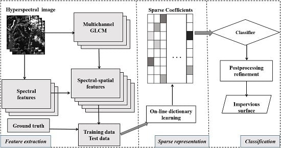
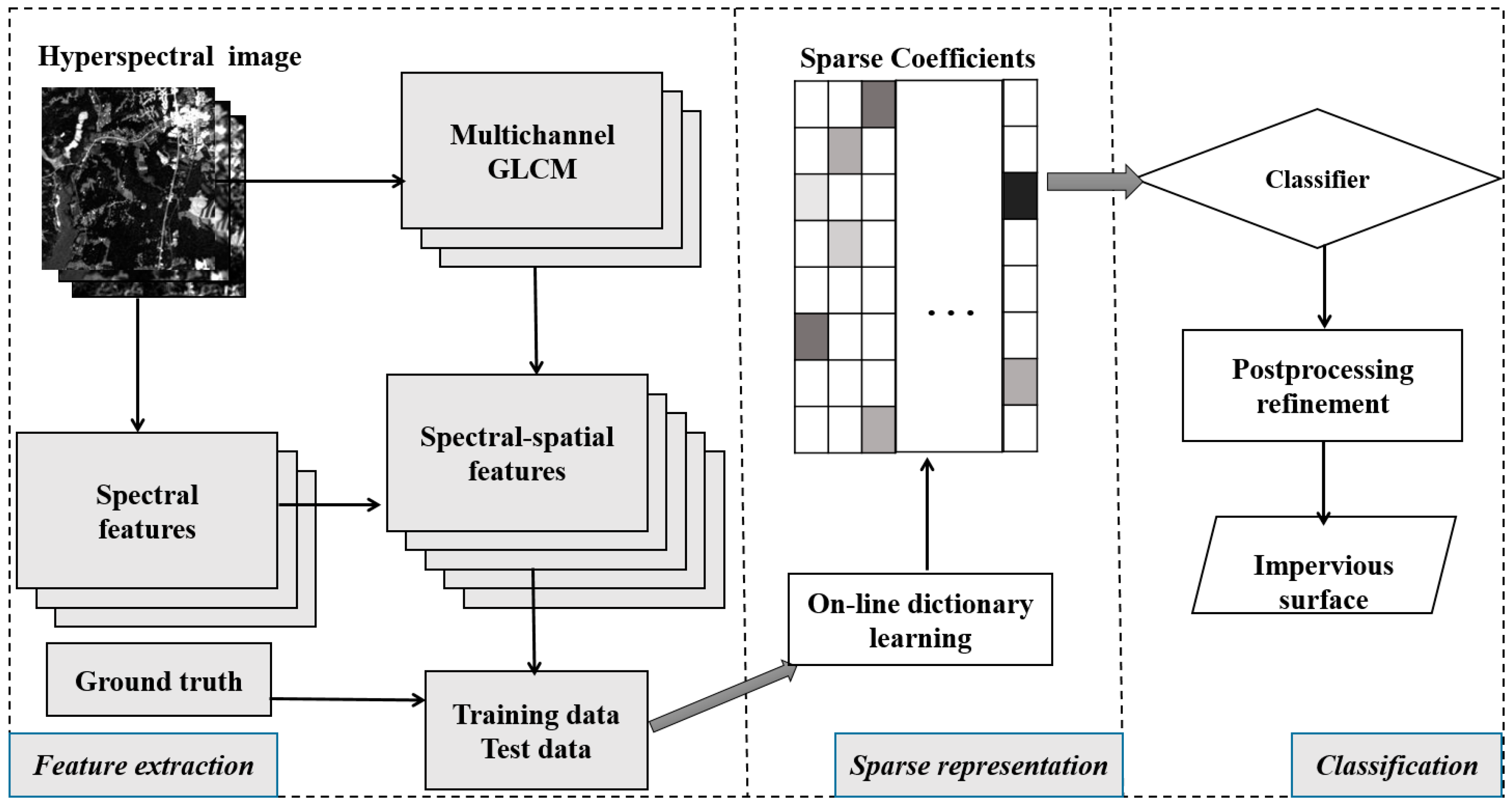
More recently, sparse representation has been applied to unmixing [29,30,31] and classification [32,33] tasks with state of the art results. However, it has been investigated less frequently to improve the impervious surface extraction accuracy. Thus, we develop a per-pixel estimation algorithm using spectral-spatial sparse representation for automatically selecting representative features in hyperspectral images. The sparse feature selection procedure can avoid overfitting and improve model performance [34]. Hyperspectral images can be compactly represented by a few atoms that carry most of the information from a certain basis vectors called a dictionary [35]. An unknown pixel is approximately represented by a sparse linear combination of atoms from the dictionary. Pixels with similar spectral-spatial properties will have similar sparse coefficients which represent the positions of selected atoms and related weight values. Therefore, the impervious surfaces areas of test samples can be determined according to the estimated sparse coefficients. The characteristics of our proposed method are listed as follows: (1) the strategy of combining the spectral features with multichannel gray level co-occurrence matrix (GLCM) spatial features can well reveal the land cover properties; (2) a spectral-spatial feature sparse coding algorithm is introduced to increase the discrimination among impervious surface, bare soil and muddy water; and (3) the proposed sparse representation model is combined with post-classification processing to further enhance impervious surface estimation performance.
The remainder of this paper is organized as follows. Section 2 presents the datasets and the proposed spectral-spatial feature sparse representation (SS-SR) and post-processing approach in detail. Section 3 illustrates the experimental results and analysis, followed by the conclusion with some suggestions for future works.
2. Materials and Methods
2.1. Dataset and Preprocessing
Medium spatial resolution hyperspectral images were widely applied in impervious surface estimation. Few papers were published on impervious surface extraction using high spatial resolution hyperspectral images. In this paper, both medium spatial resolution (Earth Observing-1 (EO-1) Hyperion datasets) and high spatial resolution (ROSIS datasets) hyperspectral images were used in the study. One scene Hyperion image (Path/Row: 15/33) was acquired on 2 October 2006. Hyperion acquires 242 bands with spectral region from 356–2577 nm. Low quality bands are removed and remaining bands are: 8–57 (427–925 nm), 79 (933 nm), 83–119 (973–1336 nm), 133–164 (1477–1790 nm), 183–184 (1982–1992 nm), and 188–220 (2032–2355 nm). Radiometric correction is performed one the image using the calibration parameter file. Radiometric calibration is performed on the image using the Environment for Visualizing Images (ENVI) Radiometric calibration module. Then, we used ENVI Fast Line-of-sight Atmospheric Analysis of Hypercubes (FLAASH) module for atmospheric correction. Two subsets of the image are extracted for impervious surface estimation (Figure 1). The two datasets are located in the south-central part of Maryland, USA. One dataset of the image has a spatial coverage of 120 × 120 pixels. The other dataset of the image contains 200 × 190 pixels. In addition, reference data are collected from the 2006 National Land Cover Database (NLCD) products [36,37,38]. Based on NLCD, the dominating land cover classes in the study area are open water, open space (impervious surface account for less than 20% of total cover), low intensity (impervious surface account for 20% to 49% of total cover), medium intensity (impervious surface account for 50% to 79% of total cover) and high intensity (impervious surface account for 80% to 100% of total cover), deciduous forest, evergreen forest, cultivated crops and woody wetlands. In this paper, two types of land cover, which are medium intensity and high intensity developed areas, are obtained to build the reference impervious surface ground truth (Figure 1). Most of the two study areas are covered with non-impervious surface.
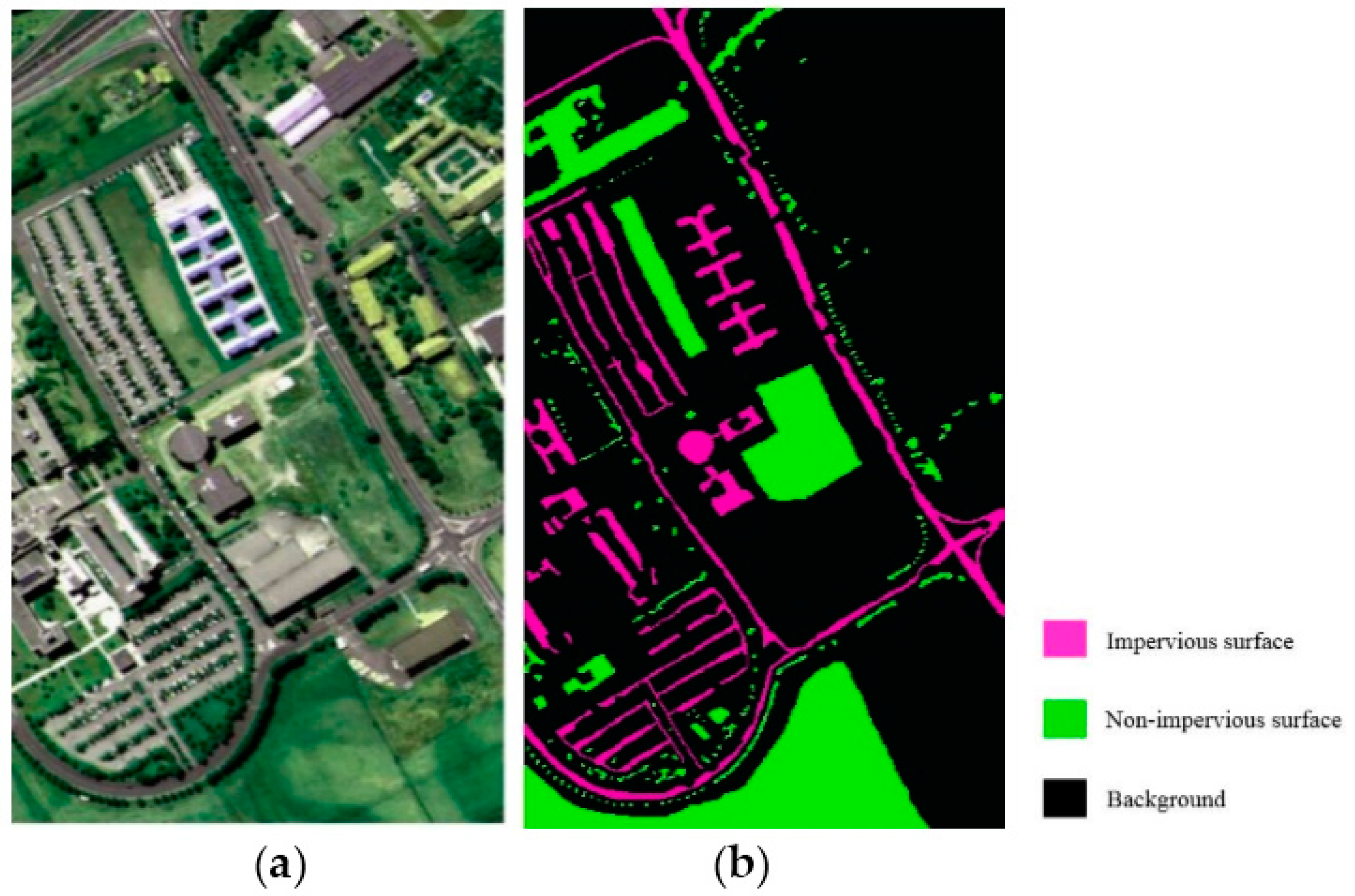
Another two images were acquired with the Reflective Optics System Imaging Spectrometer (ROSIS-03) sensor over an urban area surrounding the city of Pavia, Italy, on 8 July 2002 [27]. The original image provides 115 bands with a spectral range from 430 to 860 nm. The spatial resolution of the two datasets is 1.3 m per pixel. One of the ROSIS-03 sensor datasets was acquired near the Engineering School, University of Pavia [14]. The image has a spatial coverage of 610 × 340 pixels. Twelve spectral bands were removed due to noise, and 103 bands remained for the study. Three band false color composite image and the ground truth map are shown in Figure 2a. There are nine classes in the reference ground truth: asphalt, meadow, gravel, tree, metal sheet, bare soil, bitumen, brick and shadow. We reclassified the ground truth into two classes: impervious surface (asphalt, gravel, painted metal sheets, bitumen and self-blocking bricks) and non-impervious surface (meadows, trees and bare soil). Since shadow areas in the study area do not have corresponding ground truth, such as impervious surface (e.g., asphalt) or non-impervious surface (e.g., meadows and trees) [4], they are treated as background area in the classification. Figure 2b illustrates the reference land cover map of university of Pavia dataset.
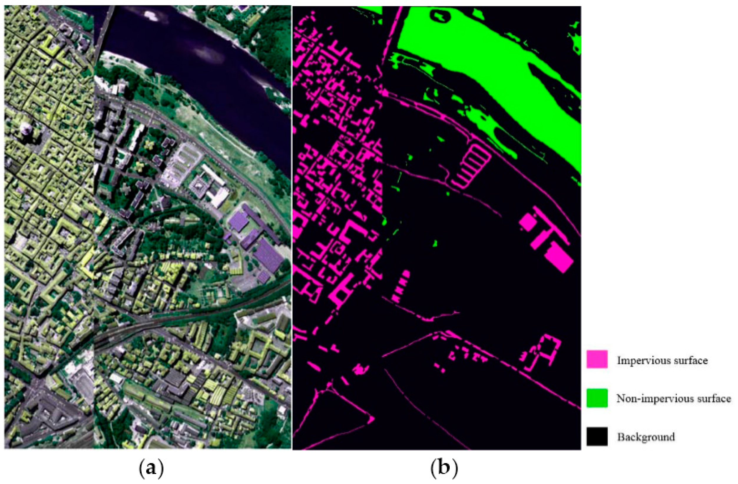
The second ROSIS-03 sensor dataset is the center of Pavia. The original image size was 1096 × 1096 pixels. A poor quality area in the image was removed. The remaining “two-part” image has a spatial coverage of 1096 × 715 pixels. Thirteen spectral bands were removed due to noise, and 102 bands remained for the study. Three bands false color composite image and the ground truth map are shown in Figure 3. There are nine classes in the original reference ground truth: bricks, asphalt, bitumen, tile, water, trees, meadows, soil and shadows. Then, bricks, asphalt, bitumen and tile are combined as impervious surface, while waters, trees, meadows and soil are combined as non-impervious surface. Figure 3b illustrates the reference land cover map of university of Pavia dataset.
2.2. Methods
Extracting impervious surface is very challenging given the high dimensional input data and the small amount of training data. In this paper, we propose a hybrid method for extracting impervious surface from hyperspectral images based on spectral-spatial sparse representation and post-classification. Different from the two-step (classification and combination) approach [4], the proposed method allows an “end to end” classification. The extraction of impervious surface is directly acquired without a combination procedure. We first extracted spectral and spatial features from hyperspectral images. We randomly selected training samples and test samples according to a certain percentage. Then, dictionary learning was carried out with an online dictionary learning algorithm [39]. Subsequently, the fast implementation of the LARS algorithm was used to learn the sparse coefficient. The least absolute shrinkage and selection operator (LASSO) algorithm [40] produces a sparse model with better prediction accuracy. We then applied the proposed sparsity-based algorithm to four hyperspectral datasets for impervious surface extraction. A majority filter was used for post-classification refinement procedure, helping to improve appearance of the estimation result. The method was finally evaluated using the reference ground truth data. A flowchart of the method is shown in Figure 4. All of the experiments were performed using MATLAB R2015b on an Intel Core i3-3220 3.3 GHz 12 GB RAM Windows 7 (64-bit) machine.
2.2.1. Feature Extraction
Normalized difference vegetation index (NDVI) and normalized difference water index (NDWI) are sensitive to vegetation and water [20]. These two extra bands were added to EO-1 Hyperion datasets to aid the spectral discrimination of vegetation and water from impervious surface and soil. Further, spatial feature is needed to reduce the classification uncertainty when only spectral feature is used. The popular gray level co-occurrence matrix (GLCM) is a spatial feature extraction approach, which is widely used for remote sensing image information extraction [41,42]. The widely used strategy is to get the GLCM from the first principal component of principal component analysis, which lost a lot of useful information. In this paper, a multichannel GLCM approach [35] is applied to analyze the spatial feature, which is more suitable for texture representation. In terms of the window size of texture measures, GLCM values are calculated with an inter-pixel distance of 1 and with three window size (3 × 3, 5 × 5, and 7 × 7). The literature calculates the statistics of the matrix in four directions (0°, 45°, 90° and 135°) and then computes the mean value. Moreover, two texture measures are chosen in the study: first moment and second moment. Extracting the first moment could be viewed as applying a low pass filter to the image, which can remove noise. The second moment feature is suitable for description of different urban land cover types [43].
2.2.2. Spectral-Spatial Sparse Representation
The problem of “curse of dimensionality”, resulting from numerous features and strong intra-feature correlations [44,45], makes the analysis of hyperspectral data fairly complicated and hard work. The fundamental scientific question is what is the appropriate representation of impervious surface that is rich enough to distinguish other land cover with hyperspectral feature. Therefore, this study introduce sparse representation theory to find a subspace for the high dimension spectral-spatial feature, which reduces the computational cost and increases feature discrimination between impervious surfaces and non-impervious surfaces. Because most pixels contain just a few materials, sparse representation models consider each pixel as a combination of just a few basis vectors from a dictionary [46]. The proposed methods involve two steps: dictionary learning and sparse representation. Let be the training set of a hyperspectral image, where m is band number and n denotes for training pixels. The linear model can be written as follows:
where D is a m × k dictionary of a few elements, αi is the sparse coefficients containing a k × 1 vector and ε is a m × 1 vector collecting the additive noise. The classical ordinary least squares (OLS) estimates are obtained by minimizing the squared error between and . The OLS estimates often have low prediction accuracy [40]. Then, the noise-tolerant sparse representation optimization is used in this paper:
where represents the ℓ0 norm of a, which computes the number of nonzero elements, and δ denotes the error tolerance due to the noise. Because of the NP-hard characteristic, the formula is difficult to solve. To tackle this issue, the ℓ0 norm can be replaced by ℓ1 norm. The optimization formula is transferred into:
where is the ℓ1 norm for the sparsity result. In theory, it has been proven that the solution of the above problem is unique when α is sparse enough, and it can have the same sparse solution instead of the ℓ0 norm. Optimizing the objective function can be written as a joint optimization problem about the dictionary D and sparse coefficients α. Depending on the particular application, dictionary learning may take different forms; we use the following equation:
where λ is a regularization parameter trading off between mean squared error and ℓ1 norm, and C is a constraint set for dictionary. In order to solve the dictionary learning problem, Julien Mairal (2010) proposed the online dictionary learning algorithm which has a low memory requirement and low computational cost [39]. Then, the fast implementation of the LARS algorithm [47] is adopted in our study to get the sparse coefficient associated with the learned dictionary. Given a matrix of X and a dictionary D, the algorithm returns a matrix of coefficients .
The algorithm is very efficient when the solution is very sparse and the problem size is reasonable. The coefficients are then used to classify the corresponding pixel using a linear support vector machine.
2.2.3. Classification Strategy and Accuracy Assessment
In this study, a hybrid approach is adopted to estimate impervious surfaces. Firstly, randomly chosen spectral-spatial sparse features and corresponding ground reference (impervious or non-impervious) are employed to train a classifier. Secondly, the classifier is directly used to predict the label (impervious or non-impervious) of test data. The test samples are classified using a linear SVM trained on the linear combination of coefficients, known as the sparse representation. In addition, post-classification refinement procedure was applied with majority filter, helping to overcome the minor salt and pepper appearance of the extraction result. Filtering is executed based on a sliding window, and the label of the central pixel is determined by the majority value of their neighboring pixels. In the study, the filter kernel is set to 3 × 3. An edge and corner pixel requires at least 4 and 3 similar value before replacement will occur. For inner pixels, the number of neighboring pixels of a similar value must be larger than 6; then a replacement can occur. The resulting value in the sliding window is assigned to the central pixel.
Five accuracy indices are adopted as the objective metrics to evaluate the accuracy of results. There are producer’s accuracy, user’s accuracy, overall accuracy (OA), average accuracy (AA), and the Kappa coefficient. The OA and Kappa are widely used to access the accuracy of impervious surface estimation [48,49]. The OA is calculated by the ratio between rightly classified impervious surface test samples and the total number of test samples. The AA is the average of the accuracy values for each class.
3. Results and Analysis
In this section, we provide a series of experimental results to evaluate the effectiveness of the proposed impervious estimation algorithms on four hyperspectral datasets. Because it takes a lot of time and labor to obtain ground truth data in reality, the experiments we designed are based on small training datasets. Support vector machine (SVM) and random forest (RF) have proven successful in extraction of impervious surface [50,51,52]. Hence, the extraction accuracies are compared visually and quantitatively with the following methods: SVM applied to spectral data with RBF kernel (SPE-SVM), SVM applied to spectral-spatial data with RBF kernel (SS-SVM), RF applied to spectral data (SPE-RF), RF applied to spectral-spatial data (SS-RF), spectral feature sparse representation (SPE-SR). For the SVM-based methods (SVM, SS-SVM) all parameters (RBF kernel parameter σ, regularization parameter C) are obtained by simple cross-validation. The optimal number of decision trees should be the first position when the kappa coefficient reaches the highest [4]. In our application, 20 decision trees are used for impervious surface extraction. The sparse regularization factor λ was allowed to take values from 0.1 to 0.9. To choose the number of dictionary atoms, values were chosen from (1/8, 1/4, 1/2) as the number of training data. The sparse representation of spectral-spatial features with these atoms is likely to exhibit discriminative capabilities.
3.1. Experiments with the Hyperion Data
As shown in Figure 1, Hyperion data refer to two datasets in this study. There are 1506 impervious surface pixels in dataset 1, and 12,894 non-impervious surface pixels. In our first experiment, 10% of the Hyperion dataset 1 are randomly used for training, and the remaining 90% are chosen for testing. The results are averaged over five runs. The images show impervious surfaces in hot pink and non-impervious surfaces in light green. The training and test data are visually illustrated in Figure 5a,b respectively. Figure 1c shows the ground truth classes. The classification maps on dataset 1 obtained from different algorithms are shown in Figure 5c–h. The circled area shows that the SS-SR yielded impervious surface closer to the reference ground truth map (Figure 1).
The estimation accuracy for impervious surface, the producer’s accuracy, user’s accuracy, overall accuracy, average accuracy, and the kappa coefficient are shown in Table 1 using different methods on the test data. In most cases, algorithms with spectral-spatial information outperforms the methods with only spectral information. The results of SPE-SVM are OA = 0.9337, and Kappa = 0.5834. The results of SS-SR are OA = 0.9402, and Kappa = 0.6570. The relatively low kappa values might be due to the training impervious surface sample size being too small to get better results. The accuracy assessment indicates that the proposed SS-SR method can produce higher accuracy than other methods in the estimation of impervious surface from hyperspectral imagery.
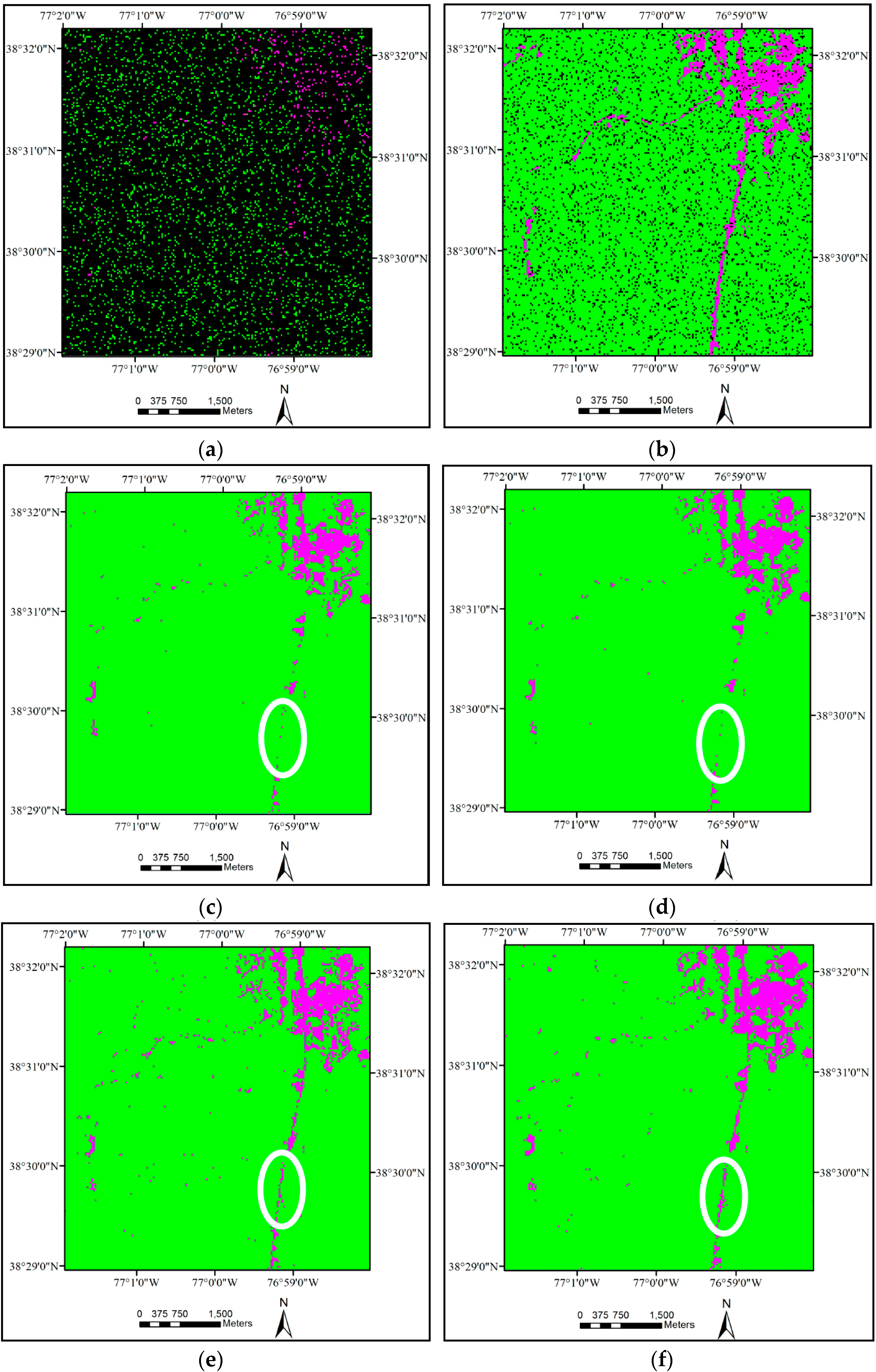
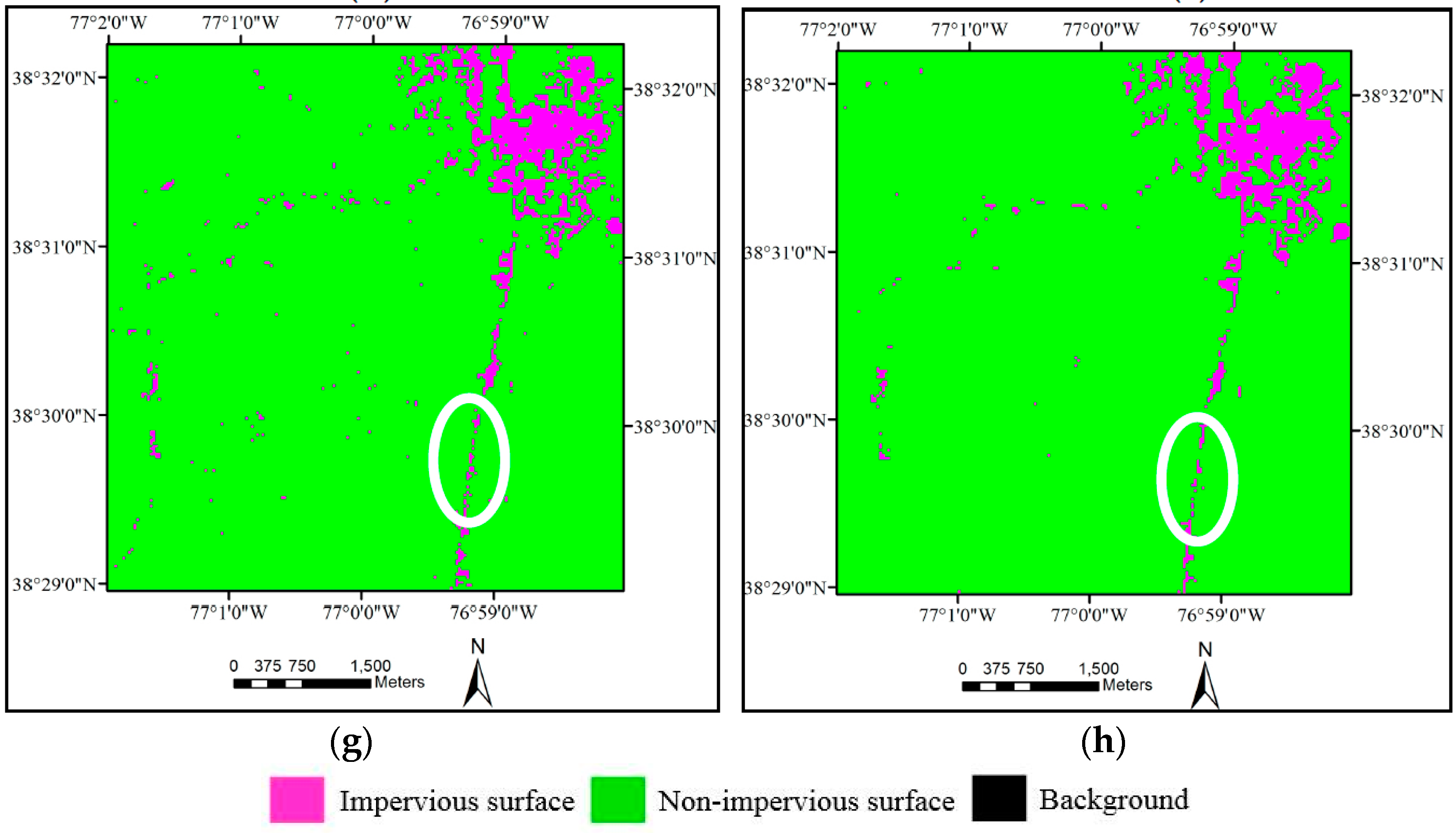
In the second experiment, there are 2747 impervious surface pixels in dataset 2, and 35,253 non-impervious surface pixels; 10% of the Hyperion dataset 2 are randomly selected for training, leaving 90% for testing. The training and testing sets are shown in Figure 6a,b, respectively. Figure 1e maps the ground-truth impervious and non-impervious surface. The circled area in Figure 6c,d illustrates the road was disconnected. The road shape of Figure 6e–h is more complete than that of Figure 6c,d. Figure 6e,f contains more “salt and pepper” noise than Figure 6g,h. Estimation maps for all algorithms depicted in Figure 6 with experiment results for the data are illustrated in Table 2.
Accuracy assessment results for Hyperion dataset 2 are shown in Table 2. The algorithms based only on spectral feature provide poor results compared with the other algorithms that take into account spatial information. The SS-SR provides better OA and Kappa results than the SS-SVM and SS-RF, which shows that SS-SR is successful in selecting discriminative spectral-spatial features of hyperspectral images. The results were OA = 0.9573 and Kappa = 0.6368.
3.2. Experiments with the University of Pavia Image
The next hyperspectral image used in our study is the University of Pavia image. About 1% of the image pixels are used for training, leaving 99% for testing. Figure 2b illustrates the ground-truth impervious and non-impervious surface. The estimation maps are presented in Figure 7c–h, and the accuracy assessment results are summarized in Table 3. Some impervious surface materials are made of rock, sand or clayish soil. Thus, impervious surfaces and soil exhibit similar spectral characteristics [53]. One can see from the circled area from Figure 7c–f that SVM and RF have difficulty in separating soil from impervious surfaces. The circled area shows bare soil pixels are wrongly classified as impervious surface. Figure 7g,h shows the visual results obtained by sparse representation method, the sparsity-based methods lead to a much finer estimation map than SVM algorithms.
We can see in Table 3 that Producer’s accuracy, User’s accuracy, OA, AA, and Kappa for the image are notably higher than the Hyperion datasets experiments. This is because the Pavia image has higher spatial resolution and lower spectral mixture. In this case, SPE-SR outperforms SPE-SVM and SPE-RF, and SS-SR outperforms SS-SVM and SS-RF. SS-SR yields the best results due to its ability to select representative spectral and spatial features.
3.3. Experiments with the Pavia Center Image
The fourth image, the Pavia center image, is also collected by the ROSIS sensor. In this experiment, around 1% of the labeled data are chosen as the training samples (Figure 8a), and the remaining 99% for testing (Figure 8b). The impervious and non-impervious surfaces estimation maps are drawn on Figure 8c–h. Figure 3b illustrates the ground-truth map. Some pixels of the lake are in a muddy state due to the lack of water circulation in the study area. This could result in stronger reflectance by water and increase the confusion between water and impervious surface. The misclassification in the extraction results of SPE-SVM and SS-SVM are due largely to the confusion between bare soil, water and impervious surface. The rectangular area depicts bare soil and muddy water pixels are recognized as impervious surface in Figure 8c–f. The confusion results of random forest mainly come from two aspects: bare soil and impervious surface, bricks and non-impervious surface. The circled area of Figure 8f shows the misclassification between bricks (impervious surface) and non-impervious surface. The proposed SPE-SR and SS-SR method can correctly recognize most of the impervious surface and remove bare soil and muddy water pixels in Figure 8g,h.
The extraction results using SPE-SVM, SS-SVM, SPE-RF, SS-RF, SPE-SR and SS-SR are summarized in Table 4. The SVM based algorithms provide poor results compared with the other algorithms. The SVM has difficulty in distinguishing muddy water from impervious surfaces using spectral-spatial features. SS-RF gets higher accuracy than SPE-RF. The SS-SR provides the best results. The results shows that SS-SR is successful in selecting discriminative spectral-spatial features of hyperspectral images.
Pavia center image was taken as a case study to show the selection of atoms from a dictionary. Figure 9 illustrates the sparse coefficients in the Pavia center image experiment. We constructed a dictionary made up of 690 atoms. After learning the dictionary, the algorithm returns a matrix of sparse coefficients, which are used as features to extract impervious surface. The coefficients represent the choice of dictionary atoms. We choose one pixel per class for impervious surface and non-impervious surface, shown in the following figures. Their locations are (732, 116) and (290, 462).
3.4. Post-Classification Refinement
Per-pixel based methods would result in the so-called “salt and pepper” effect in the estimation results. In this paper, a majority filter was used to weaken the “salt and pepper” appearance of the extraction results. The post-classification method was carried out directly on the four SS-SR classification results. Visual inspection shows that our method could further improve the impervious surface estimation. The salt and pepper effect can be clearly seen in Figure 10a,b,d,e. Compared with the raw result, the effect in Hyperion dataset 1 and dataset 2 is partly corrected by the majority filter. Meanwhile, a lot of misclassifications occurred between bare soil, muddy water and impervious surfaces, which can be seen in Figure 10g,h,j,k. The misclassifications are partly corrected by the post-classification refinement.
An accuracy assessment was conducted to compare the results. In the Hyperion dataset 1 experiment, the SS-SR with majority filter yields kappa of 0.6663, with the SPE-SVM kappa of 0.5834. In the University of Pavia experiment, the SS-SR with post-classification yields kappa of 0.9919, with the SPE-SVM kappa of 0.9519. The results of OA and Kappa indicate that all of the images achieved a relatively higher accuracy. The two other experiments also prove the superiority of this algorithm. The improvements could be due to the spatial information in the neighbor pixels being effectively used in the approach. It is demonstrated that the post-classification approach is capable of providing more accurate results than the raw classification. The detailed statistical results are presented in Table 5.
4. Discussion
4.1. The Classification Accuracy for Impervious Surface
Impervious surface, bare soil and muddy water from wide band reflectance data of multispectral remote sensing images are not spectrally distinct. It is difficult to distinguish impervious surface from bare soil with similar spectral signatures. Due to the urban land cover diversity and the spectral confusion of low spectral remote sensing images, hyperspectral images have become a promising approach to improve impervious surface estimation. In this study, EO-1 Hyperion and ROSIS image datasets were used to characterize and quantify the spatial patterns of impervious surfaces. The spectral and spatial features were combined by layer stacking method, which is easy to implement. In general, the combined use of hyperspectral images spectral and spatial features improved the Overall accuracy and Kappa compared to using only spectral information for extracting impervious surfaces. The spatial resolution of Hyperion images is coarse for mapping per-pixel impervious surface, especially in the complex urban land surface. The impervious surface areas are often underestimated in the rural area when using Hyperion datasets. Possible reasons could be that most of the land is covered by non-impervious surfaces in the rural area, the imbalanced impervious and non-impervious surfaces lead to the underestimation. The spatial resolution of ROSIS images is suitable for extracting per-pixel impervious surface. The higher extraction accuracy of ROSIS datasets than that of Hyperion is probably due to the higher spatial resolution of the former, which makes it more suitable to detect impervious surface details. When bare soil and muddy water are mixed with impervious surfaces, they are difficult to separate by RBF kernel SVM. The results of random forest are slightly less accurate than SS-SR, but run faster. In this study, it is found that the confusion between impervious and non-impervious surface (such as bare soil, etc.) can be significantly reduced using spectral-spatial sparse representation and majority filter. The results imply that our method of impervious surface estimation is consistent, and thus has the potential to be applied to other hyperspectral remote sensing images. Another issue is related to post-classification refinement. The size of majority filter kernel is an important parameter. When the land cover is complex, it is suitable to use a small window. This research shows that complete extraction of impervious surfaces are still difficult and post-processing methods are needed to further separate them from non-impervious surfaces. The increased accuracy of the hybrid approach could promote the development of land use change, heat island effect and urban expansion research.
4.2. The Computational Costs
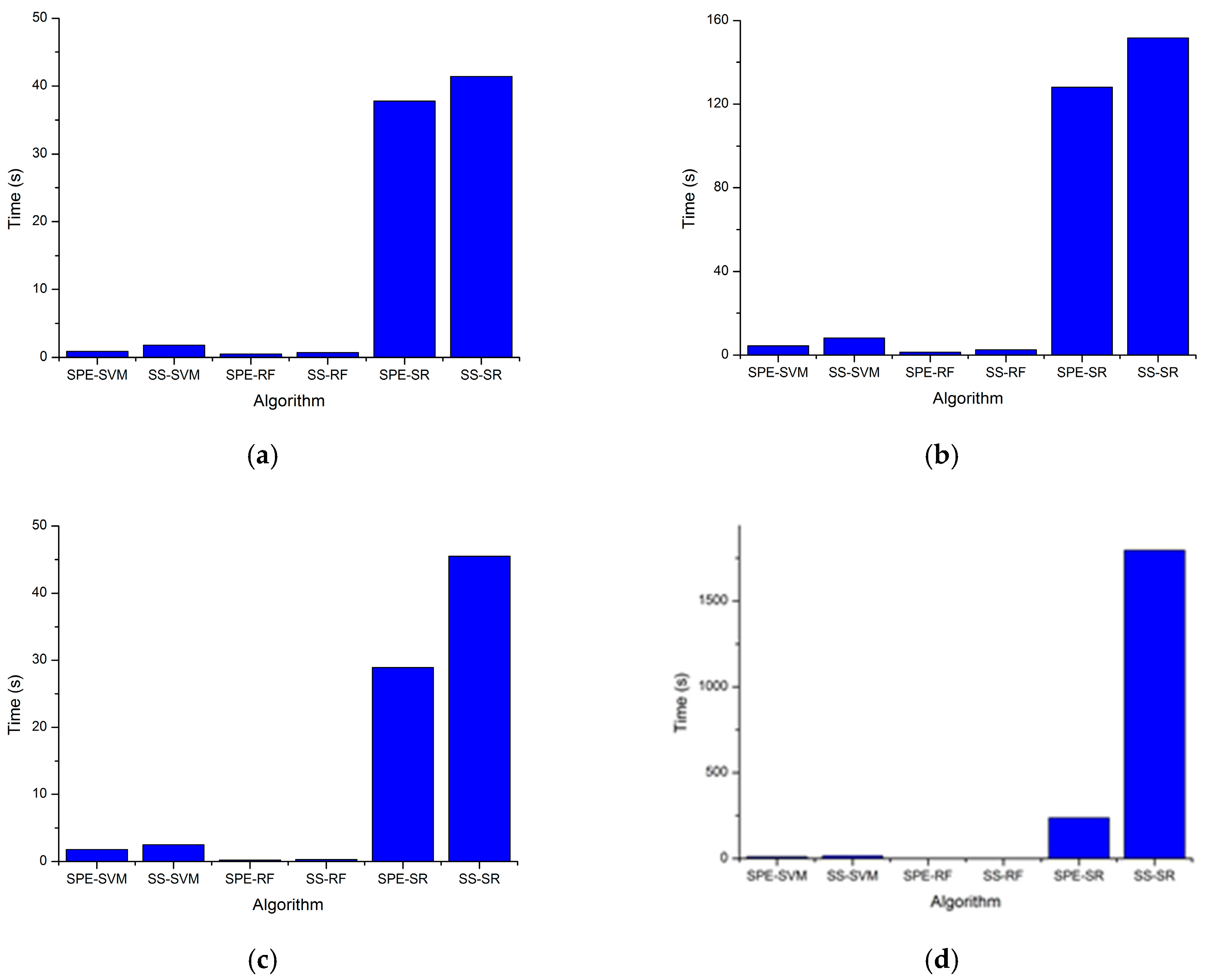
The computational costs were evaluated on four hyperspectral datasets. All of the experiments were performed using MATLAB R2015b. The results are illustrated in Figure 11. The computation times of SPE-SVM, SS-SVM, SPE-RF, SS-RF, SPE-SR and SS-SR were gradually increasing. We can see in Figure 11 that RF algorithm cost the shortest time. Compared with SVM and RF, the running time of SPE-SR and SS-SR were relatively long, but still the general computer can afford. Algorithms with spectral-spatial features took longer time than that with only spectral features. The calculation time of the majority filter is generally not more than 1 s. It is worth noting that the computational costs mainly from the computational complexity of the sparse representation algorithms. Further refinements can be done by optimizing the algorithm and adopting high performance computing hardware.
5. Conclusions
The major contribution of this study is to improve impervious surface estimation from hyperspectral images using sparse representation and post-processing refinement. To test the effectiveness of the SS-SR approach, four hyperspectral datasets were used to estimate the impervious surface. In the study, producer’s accuracy, user’s accuracy, overall accuracy (OA), average accuracy (AA), and the Kappa were used for accuracy assessment. The results show SS-SR yields better results due to its ability to select representative spectral and spatial features. The post-classification approach is capable of providing more accurate results than the raw classification. The combined use of SS-SR and majority filter algorithm is effective to improve the impervious surface mapping, by reducing the confusions between impervious surface and bare soil, as well as muddy water surface. Experimental results on four hyperspectral datasets demonstrate the superiority of the proposed hybrid method over several well-known impervious surface estimation algorithms. Compared with traditional SPE-SVM, the integration of SS-SR with majority filter enhanced the average kappa by 8.27% (EO-1 Hyperion datasets) and 6.23% (ROSIS Pavia datasets). Our hybrid approach increased the average kappa by 7.60% (EO-1 Hyperion datasets) and 2.35% (ROSIS Pavia datasets) compared with classical SPE-RF. Although the impervious surfaces can be extracted with relatively higher accuracy using our approach, the estimation process is found to be time-consuming. In the future study, we intend to focus on the computationally-efficient implementation of the proposed method.
Acknowledgments
This work was partly supported by the National Natural Science Foundation of China (61303128), Natural Science Foundation of Hebei Province (F2013203220 and F2017203169), Key Foundation of Hebei Educational Committee (ZD2017080), Youth Foundation of Hebei Educational Committee (QN2017146), Science and Technology Foundation for Returned Overseas People of Hebei Province (CL201621), and the Special Foundation for Basic Research Program of Yanshan University (16LGB009). The authors would like to thank the USGS for providing EO-1 Hyperion and NLCD dataset; P. Gamba for providing the ROSIS data over Pavia, Italy; Lin, C. for providing the LIBSVM toolbox; and Abhishek Jaiantilal for providing the Random Forest code. Additionally, we also thank the editor and the anonymous reviewers for their constructive comments and suggestions.
Author Contributions
Shuai Liu conceived and designed the paper, performed the experiments, and finished the manuscript. Guanghua Gu designed and revised the paper.
Conflicts of Interest
The authors declare no conflict of interest.
References
- Weng, Q. Remote sensing of impervious surfaces in the urban areas: Requirements, methods, and trends. Remote Sens. Environ. 2012, 117, 34–49. [Google Scholar] [CrossRef]
- Fan, F.; Fan, W.; Weng, Q. Improving urban impervious surface mapping by linear spectral mixture analysis and using spectral indices. Can. J. Remote Sens. 2015, 41, 1–10. [Google Scholar] [CrossRef]
- Ma, Q.; He, C.; Wu, J.; Liu, Z.; Zhang, Q.; Sun, Z. Quantifying spatiotemporal patterns of urban impervious surfaces in China: An improved assessment using nighttime light data. Landsc. Urban Plan. 2014, 130, 36–49. [Google Scholar] [CrossRef]
- Zhang, Y.; Zhang, H.; Lin, H. Improving the impervious surface estimation with combined use of optical and sar remote sensing images. Remote Sens. Environ. 2014, 141, 155–167. [Google Scholar] [CrossRef]
- Shao, Z.; Liu, C. The integrated use of DMSP-OLS nighttime light and modis data for monitoring large-scale impervious surface dynamics: A case study in the yangtze river delta. Remote Sens. 2014, 6, 9359–9378. [Google Scholar] [CrossRef]
- Liu, X.; Hu, G.; Ai, B.; Li, X.; Shi, Q. A normalized urban areas composite index (NUACI) based on combination of DMSP-Ols and MODIS for mapping impervious surface area. Remote Sens. 2015, 7, 17168–17189. [Google Scholar] [CrossRef]
- Jing, W.; Yang, Y.; Yue, X.; Zhao, X. Mapping urban areas with integration of DMSP/OLS nighttime light and MODIS data using machine learning techniques. Remote Sens. 2015, 7, 12419–12439. [Google Scholar] [CrossRef]
- Zhou, Y.; Smith, S.J.; Elvidge, C.D.; Zhao, K.; Thomson, A.; Imhoff, M. A cluster-based method to map urban area from DMSP/OLS nightlights. Remote Sens. Environ. 2014, 147, 173–185. [Google Scholar] [CrossRef]
- Wang, Z.; Gang, C.; Li, X.; Chen, Y.; Li, J. Application of a Normalized Difference Impervious Index (NDII) to extract urban impervious surface features based on landsat tm images. Int. J. Remote Sens. 2015, 36, 1055–1069. [Google Scholar] [CrossRef]
- Zhang, L.; Weng, Q. Annual dynamics of impervious surface in the pearl river delta, china, from 1988 to 2013, using time series landsat imagery. ISPRS J. Photogramm. Remote Sens. 2016, 113, 86–96. [Google Scholar] [CrossRef]
- Li, L.; Lu, D.; Kuang, W. Examining urban impervious surface distribution and its dynamic change in Hangzhou metropolis. Remote Sens. 2016, 8, 1–20. [Google Scholar] [CrossRef]
- Song, X.P.; Sexton, J.O.; Huang, C.; Channan, S.; Townshend, J.R. Characterizing the magnitude, timing and duration of urban growth from time series of landsat-based estimates of impervious cover. Remote Sens. Environ. 2016, 175, 1–13. [Google Scholar] [CrossRef]
- Tang, F.; Xu, H.Q. Comparison of performances in retrieving impervious surface between hyperspectral (hyperion) and multispectral (TM/ETM+) images. Spectrosc. Spectr. Anal. 2014, 34, 1075–1080. [Google Scholar]
- Tan, K.; Jin, X.; Du, Q.; Du, P.J. Modified multiple endmember spectral mixture analysis for mapping impervious surfaces in urban environments. J. Appl. Remote Sens. 2014, 8, 085096. [Google Scholar] [CrossRef]
- Shuai, L.; Qi, L. Composite kernel support vector regression model for hyperspectral image impervious surface extraction. J. Remote Sens. 2016, 20, 420–430. [Google Scholar]
- Ridd, M.K. Exploring a vis (vegetation-impervious surface-soil) model for urban ecosystem analysis through remote sensing: Comparative anatomy for cities. Int. J. Remote Sens. 1995, 16, 2165–2185. [Google Scholar] [CrossRef]
- Wu, C.; Murray, A.T. Estimating impervious surface distribution by spectral mixture analysis. Remote Sens. Environ. 2003, 84, 493–505. [Google Scholar] [CrossRef]
- Deng, C.; Wu, C. A spatially adaptive spectral mixture analysis for mapping subpixel urban impervious surface distribution. Remote Sens. Environ. 2013, 133, 62–70. [Google Scholar] [CrossRef]
- Deng, Y.; Wu, C. Development of a class-based multiple endmember spectral mixture analysis (C-MESMA) approach for analyzing urban environments. Remote Sens. 2016, 8, 349. [Google Scholar] [CrossRef]
- Xu, H. Rule-based impervious surface mapping using high spatial resolution imagery. Int. J. Remote Sens. 2013, 34, 27–44. [Google Scholar] [CrossRef]
- Shao, Z.; Fu, H.; Fu, P.; Yin, L. Mapping urban impervious surface by fusing optical and sar data at the decision level. Remote Sens. 2016, 8, 945. [Google Scholar] [CrossRef]
- Okujeni, A.; van der Linden, S.; Hostert, P. Extending the vegetation-impervious-soil model using simulated enmap data and machine learning. Remote Sens. Environ. 2015, 158, 69–80. [Google Scholar] [CrossRef]
- Weng, Q.; Hu, X.; Lu, D. Extracting impervious surfaces from medium spatial resolution multispectral and hyperspectral imagery: A comparison. Int. J. Remote Sens. 2008, 29, 3209–3232. [Google Scholar] [CrossRef]
- Roberts, D.A.; Gardner, M.; Church, R.; Ustin, S.; Scheer, G.; Green, R.O. Mapping chaparral in the santa monica mountains using multiple endmember spectral mixture models. Remote Sens. Environ. 1998, 65, 267–279. [Google Scholar] [CrossRef]
- Fan, F.; Deng, Y. Enhancing endmember selection in multiple endmember spectral mixture analysis (MESMA) for urban impervious surface area mapping using spectral angle and spectral distance parameters. Int. J. Appl. Earth Obs. 2014, 33, 290–301. [Google Scholar] [CrossRef]
- Van der Linden, S.; Hostert, P. The influence of urban structures on impervious surface maps from airborne hyperspectral data. Remote Sens. Environ. 2009, 113, 2298–2305. [Google Scholar] [CrossRef]
- Fauvel, M.; Tarabalka, Y.; Benediktsson, J.A.; Chanussot, J.; Tilton, J.C. Advances in spectral-spatial classification of hyperspectral images. Proc. IEEE 2013, 101, 652–675. [Google Scholar] [CrossRef]
- Zhang, H.; Lin, H.; Li, Y.; Zhang, Y.; Fang, C. Mapping urban impervious surface with dual-polarimetric sar data: An improved method. Landsc. Urban Plan. 2016, 151, 55–63. [Google Scholar] [CrossRef]
- Iordache, M.D.; Bioucas-Dias, J.M.; Plaza, A. Total variation spatial regularization for sparse hyperspectral unmixing. IEEE Trans. Geosci. Remote Sens. 2012, 50, 4484–4502. [Google Scholar] [CrossRef]
- Wei, T.; Zhenwei, S.; Ying, W.; Changshui, Z. Sparse unmixing of hyperspectral data using spectral a priori information. IEEE Trans. Geosci. Remote Sens. 2015, 53, 770–783. [Google Scholar]
- Iordache, M.D.; Bioucas-Dias, J.M.; Plaza, A.; Somers, B. Music-csr: Hyperspectral unmixing via multiple signal classification and collaborative sparse regression. IEEE Trans. Geosci. Remote Sens. 2014, 52, 4364–4382. [Google Scholar] [CrossRef]
- Yi, C.; Nasrabadi, N.M.; Tran, T.D. Hyperspectral image classification using dictionary-based sparse representation. IEEE Trans. Geosci. Remote Sens. 2011, 49, 3973–3985. [Google Scholar]
- Du, P.; Xue, Z.; Li, J.; Plaza, A. Learning discriminative sparse representations for hyperspectral image classification. IEEE J. Sel. Top. Signal Process. 2015, 9, 1089–1104. [Google Scholar] [CrossRef]
- Gui, J.; Sun, Z.; Ji, S.; Tao, D.; Tan, T. Feature selection based on structured sparsity: A comprehensive study. IEEE Trans. Neural Netw. Learn. 2016, 25, 1–18. [Google Scholar] [CrossRef] [PubMed]
- Huang, X.; Liu, X.; Zhang, L. A multichannel gray level co-occurrence matrix for multi/hyperspectral image texture representation. Remote Sens. 2014, 6, 8424–8445. [Google Scholar] [CrossRef]
- Xian, G.; Homer, C. Updating the 2001 national land cover database impervious surface products to 2006 using landsat imagery change detection methods. Remote Sens. Environ. 2010, 114, 1676–1686. [Google Scholar] [CrossRef]
- Nagel, P.; Yuan, F. High-resolution land cover and impervious surface classifications in the twin cities metropolitan area with naip imagery. Photogramm. Eng. Remote Sens. 2016, 82, 63–71. [Google Scholar] [CrossRef]
- Deng, C. Incorporating endmember variability into linear unmixing of coarse resolution imagery: Mapping large-scale impervious surface abundance using a hierarchically object-based spectral mixture analysis. Remote Sens. 2015, 7, 9205–9229. [Google Scholar] [CrossRef]
- Mairal, J.; Bach, F.; Ponce, J.; Sapiro, G. Online learning for matrix factorization and sparse coding. J. Mach. Learn. Res. 2010, 11, 19–60. [Google Scholar]
- Tibshirani, R. Regression shrinkage and selection via the lasso. J. R. Stat. Soc. B 1996, 58, 267–288. [Google Scholar]
- Su, H.; Yong, B.; Du, P.; Liu, H.; Chen, C.; Liu, K. Dynamic classifier selection using spectral-spatial information for hyperspectral image classification. J. Appl. Remote Sens. 2014, 8, 085095. [Google Scholar] [CrossRef]
- Li, N.; Bruzzone, L.; Chen, Z.; Liu, F. A novel technique based on the combination of labeled co-occurrence matrix and variogram for the detection of built-up areas in high-resolution sar images. Remote Sens. 2014, 6, 3857–3878. [Google Scholar] [CrossRef]
- Puissant, A.; Hirsch, J.; Weber, C. The utility of texture analysis to improve per-pixel classification for high to very high spatial resolution imagery. Int. J. Remote Sens. 2005, 26, 733–745. [Google Scholar] [CrossRef]
- Melgani, F.; Bruzzone, L. Classification of hyperspectral remote sensing images with support vector machines. IEEE Trans. Geosci. Remote Sens. 2004, 42, 1778–1790. [Google Scholar] [CrossRef]
- Sun, W.; Jiang, M.; Li, W.; Liu, Y. A symmetric sparse representation based band selection method for hyperspectral imagery classification. Remote Sens. 2016, 8, 238. [Google Scholar] [CrossRef]
- Charles, A.S.; Olshausen, B.A.; Rozell, C.J. Learning sparse codes for hyperspectral imagery. IEEE J. Sel. Top. Signal Process. 2011, 5, 963–978. [Google Scholar] [CrossRef]
- Efron, B.; Hastie, T.; Johnstone, I.; Tibshirani, R. Least angle regression. Ann. Stat. 2004, 32, 407–499. [Google Scholar]
- Hu, X.; Weng, Q. Impervious surface area extraction from ikonos imagery using an object-based fuzzy method. Geocarto Int. 2010, 26, 3–20. [Google Scholar] [CrossRef]
- Kotarba, A.Z.; Aleksandrowicz, S. Impervious surface detection with nighttime photography from the international space station. Remote Sens. Environ. 2016, 176, 295–307. [Google Scholar] [CrossRef]
- Li, E.; Du, P.; Samat, A.; Xia, J.; Che, M. An automatic approach for urban land-cover classification from Landsat-8 OLI data. Int. J. Remote Sens. 2015, 36, 5983–6007. [Google Scholar] [CrossRef]
- Samsudin, S.H.; Shafri, H.Z.M.; Hamedianfar, A.; Mansor, S. Spectral feature selection and classification of roofing materials using field spectroscopy data. J. Appl. Remote Sens. 2015, 9, 095079. [Google Scholar] [CrossRef]
- Fernandez, I.; Aguilar, F.J.; Aguilar, M.A.; Flor Alvarez, M. Influence of data source and training size on impervious surface areas classification using vhr satellite and aerial imagery through an object-based approach. IEEE J. Sel. Top. Appl. Earth Obs. Remote Sens. 2014, 7, 4681–4691. [Google Scholar] [CrossRef]
- Xu, H.Q.; Wang, M.Y. Remote sensing-based retrieval of ground impervious surfaces. J. Remote Sens. 2016, 20, 1270–1289. [Google Scholar]
Figure 1.
The geographic location of the Hyperion data: (a) true color composite image; (b) dataset 1; (c) dataset 1 ground truth; (d) dataset 2; and (e) dataset 2 ground truth.
Figure 1.
The geographic location of the Hyperion data: (a) true color composite image; (b) dataset 1; (c) dataset 1 ground truth; (d) dataset 2; and (e) dataset 2 ground truth.

Figure 2.
University of Pavia: (a) false color composite image; and (b) the reference image.

Figure 3.
Center of Pavia: (a) false color composite image; and (b) the reference image.

Figure 4.
The flowchart of SS-SR and Post-processing based impervious surface estimation.

Figure 5.
Hyperion dataset 1: (a) training data; and (b) test data. Estimation maps obtained by: (c) SVM applied to spectral data with RBF kernel (SPE-SVM); (d) SVM applied to spectral-spatial data with RBF kernel (SS-SVM); (e) RF applied to spectral data (SPE-RF); (f) RF applied to spectral-spatial data (SS-RF); (g) spectral feature sparse representation (SPE-SR); and (h) spectral-spatial feature sparse representation (SS-SR).

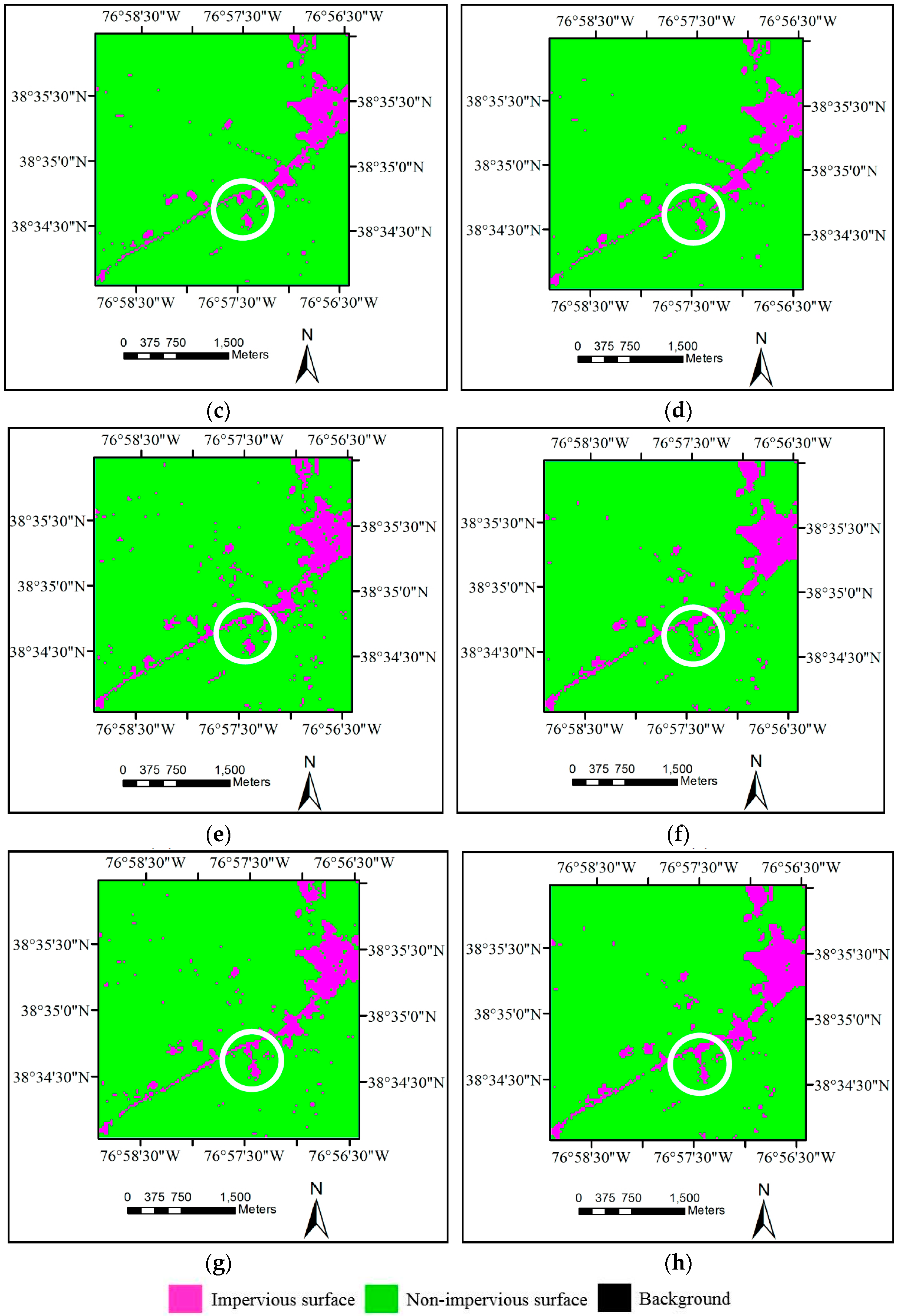
Figure 6.
Hyperion dataset 2: (a) training data; and (b) test data. Estimation maps obtained by: (c) SPE-SVM; (d) SS-SVM; (e) SPE-RF; (f) SS-RF; (g) SPE-SR; and (h) SS-SR.
Figure 6.
Hyperion dataset 2: (a) training data; and (b) test data. Estimation maps obtained by: (c) SPE-SVM; (d) SS-SVM; (e) SPE-RF; (f) SS-RF; (g) SPE-SR; and (h) SS-SR.


Figure 7.
University of Pavia image: (a) training data; and (b) test data. Estimation maps obtained by: (c) SPE-SVM; (d) SS-SVM; (e) SPE-RF; (f) SS-RF; (g) SPE-SR; and (h) SS-SR.
Figure 7.
University of Pavia image: (a) training data; and (b) test data. Estimation maps obtained by: (c) SPE-SVM; (d) SS-SVM; (e) SPE-RF; (f) SS-RF; (g) SPE-SR; and (h) SS-SR.
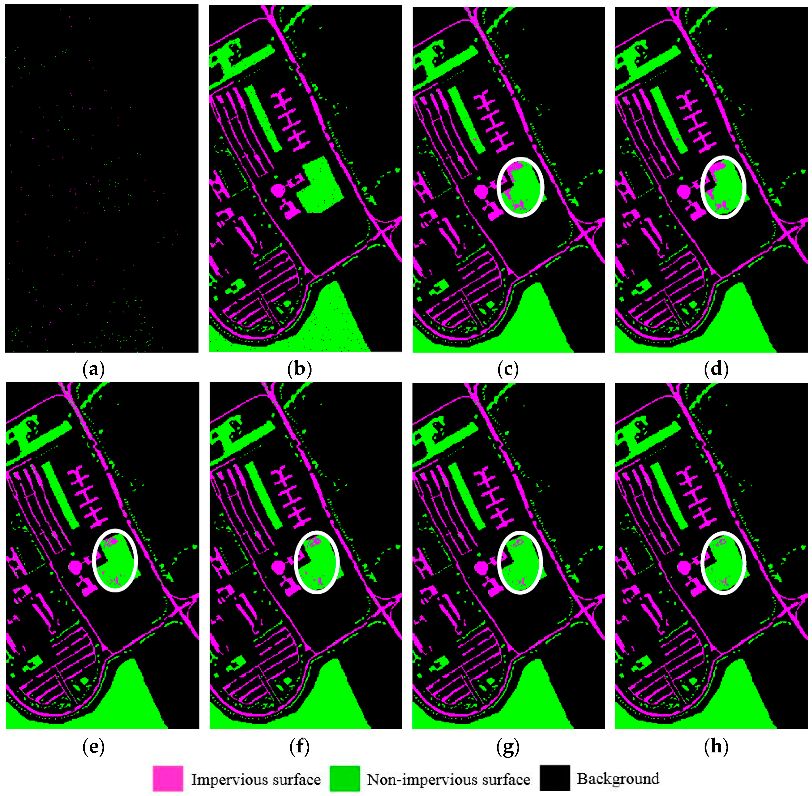
Figure 8.
Pavia center image: (a) training data; and (b) test data. Estimation maps obtained by: (c) SPE-SVM; (d) SS-SVM; (e) SPE-RF; (f) SS-RF; (g) SPE-SR; and (h) SS-SR.
Figure 8.
Pavia center image: (a) training data; and (b) test data. Estimation maps obtained by: (c) SPE-SVM; (d) SS-SVM; (e) SPE-RF; (f) SS-RF; (g) SPE-SR; and (h) SS-SR.

Figure 9.
Estimated sparse coefficients for impervious surface and non-impervious surface in the Pavia center image: (a) coefficient of pixel (732, 116); and (b) coefficient of pixel (290, 462).
Figure 9.
Estimated sparse coefficients for impervious surface and non-impervious surface in the Pavia center image: (a) coefficient of pixel (732, 116); and (b) coefficient of pixel (290, 462).
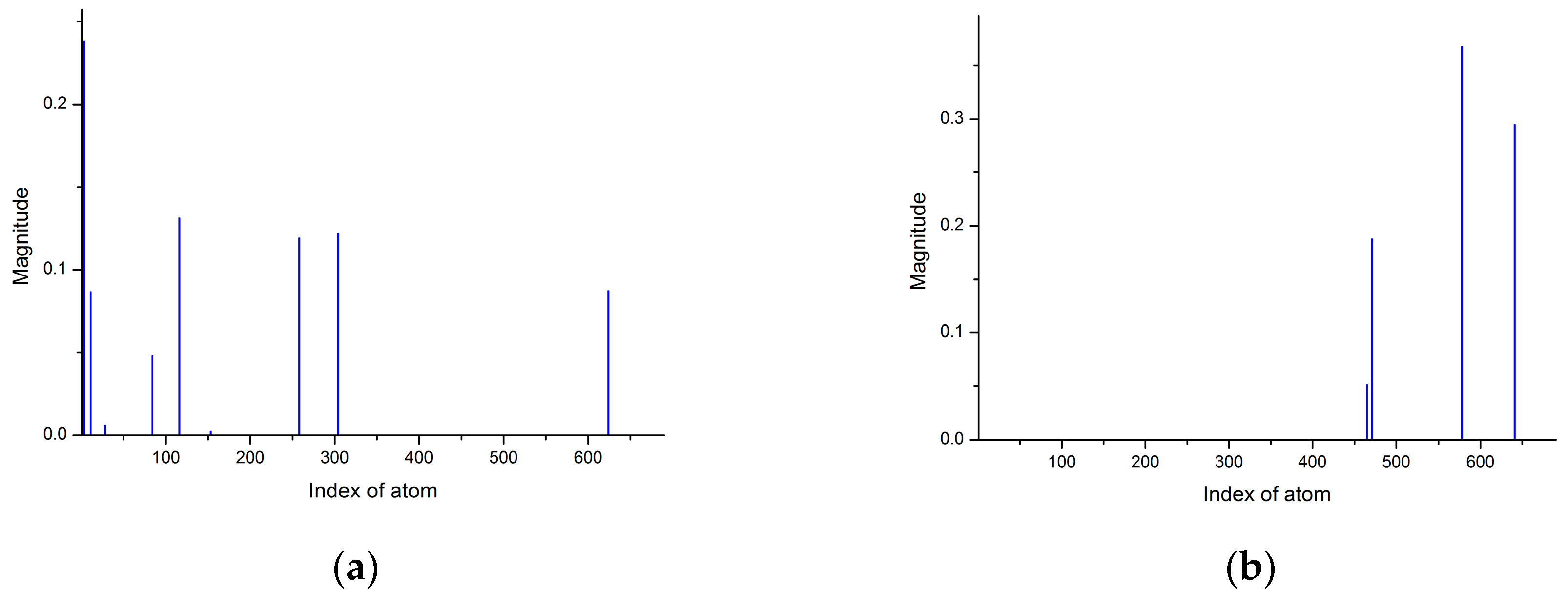
Figure 10.
Classification images: (a) SPE-SVM; (b) SPE-RF; (c) SS-SR with post-classification refinement; (d) SPE-SVM; (e) SPE-RF; (f) SS-SR with post-classification refinement; (g) SPE-SVM; (h) SPE-RF; (i) SS-SR with post-classification refinement; (j) SPE-SVM; (k) SPE-RF; and (l) SS-SR with post-classification refinement.
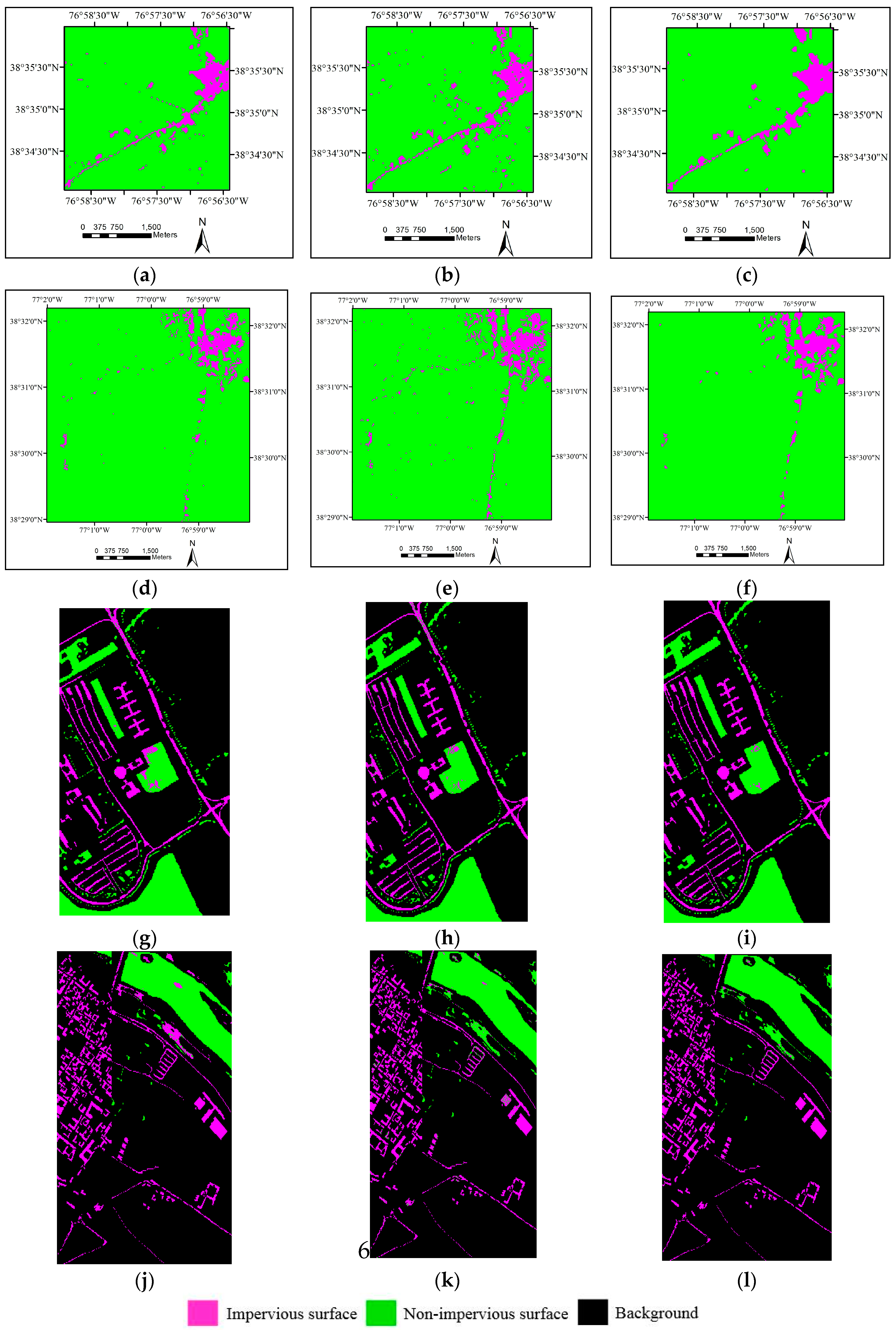
Figure 11.
Computation time of different algorithms: (a) Hyperion dataset 1; (b) Hyperion dataset 2; (c) University of Pavia; and (d) Pavia center.
Figure 11.
Computation time of different algorithms: (a) Hyperion dataset 1; (b) Hyperion dataset 2; (c) University of Pavia; and (d) Pavia center.

Table 1.
Accuracy assessment for Hyperion dataset 1.
| SPE-SVM | SS-SVM | SPE-RF | SS-RF | SPE-SR | SS-SR | |
|---|---|---|---|---|---|---|
| Producer’s Accuracy | 0.513 | 0.534 | 0.599 | 0.633 | 0.573 | 0.636 |
| User’s Accuracy | 0.777 | 0.784 | 0.697 | 0.729 | 0.778 | 0.754 |
| OA | 0.934 | 0.936 | 0.931 | 0.937 | 0.938 | 0.940 |
| AA | 0.748 | 0.759 | 0.784 | 0.803 | 0.777 | 0.806 |
| Kappa | 0.583 | 0.602 | 0.606 | 0.643 | 0.627 | 0.657 |
Table 2.
Accuracy assessment for Hyperion dataset 2.
| SPE-SVM | SS-SVM | SPE-RF | SS-RF | SPE-SR | SS-SR | |
|---|---|---|---|---|---|---|
| Producer’s Accuracy | 0.459 | 0.496 | 0.504 | 0.634 | 0.551 | 0.596 |
| User’s Accuracy | 0.790 | 0.788 | 0.672 | 0.689 | 0.708 | 0.779 |
| OA | 0.952 | 0.954 | 0.946 | 0.953 | 0.951 | 0.957 |
| AA | 0.725 | 0.743 | 0.742 | 0.806 | 0.767 | 0.779 |
| Kappa | 0.557 | 0.585 | 0.548 | 0.635 | 0.594 | 0.637 |
Table 3.
Accuracy assessment for University of Pavia image.
| SPE-SVM | SS-SVM | SPE-RF | SS-RF | SPE-SR | SS-SR | |
|---|---|---|---|---|---|---|
| Producer’s Accuracy | 0.972 | 0.972 | 0.989 | 0.990 | 0.993 | 0.996 |
| User’s Accuracy | 0.993 | 0.996 | 0.981 | 0.992 | 0.983 | 0.993 |
| OA | 0.978 | 0.980 | 0.981 | 0.989 | 0.984 | 0.993 |
| AA | 0.980 | 0.983 | 0.978 | 0.988 | 0.980 | 0.991 |
| Kappa | 0.952 | 0.957 | 0.959 | 0.976 | 0.965 | 0.984 |
Table 4.
Accuracy assessment for Pavia center image.
| SPE-SVM | SS-SVM | SPE-RF | SS-RF | SPE-SR | SS-SR | |
|---|---|---|---|---|---|---|
| Producer’s Accuracy | 0.911 | 0.910 | 0.985 | 0.989 | 0.989 | 0.990 |
| User’s Accuracy | 0.902 | 0.901 | 0.991 | 0.990 | 0.989 | 0.996 |
| OA | 0.951 | 0.951 | 0.987 | 0.989 | 0.988 | 0.992 |
| AA | 0.956 | 0.955 | 0.987 | 0.989 | 0.988 | 0.992 |
| Kappa | 0.902 | 0.901 | 0.973 | 0.978 | 0.975 | 0.984 |
Table 5.
Accuracy assessment for impervious surface estimation using different algorithm.
| OA Kappa (SPE-SVM) | OA Kappa (SS-SVM) | OA Kappa (SPE-RF) | OA Kappa (SS-RF) | OA Kappa (Our Hybrid Approach) | ||||||
|---|---|---|---|---|---|---|---|---|---|---|
| Hyperion dataset 1 | 0.934 | 0.583 | 0.936 | 0.602 | 0.931 | 0.606 | 0.937 | 0.643 | 0.943 | 0.666 |
| Hyperion dataset 2 | 0.952 | 0.557 | 0.953 | 0.585 | 0.946 | 0.548 | 0.953 | 0.635 | 0.958 | 0.640 |
| University of Pavia | 0.978 | 0.952 | 0.980 | 0.957 | 0.981 | 0.959 | 0.989 | 0.976 | 0.996 | 0.992 |
| Pavia center image | 0.951 | 0.902 | 0.951 | 0.901 | 0.987 | 0.973 | 0.989 | 0.978 | 0.993 | 0.987 |
© 2017 by the authors. Licensee MDPI, Basel, Switzerland. This article is an open access article distributed under the terms and conditions of the Creative Commons Attribution (CC BY) license (http://creativecommons.org/licenses/by/4.0/).
Share and Cite
MDPI and ACS Style
Liu, S.; Gu, G. Improving the Impervious Surface Estimation from Hyperspectral Images Using a Spectral-Spatial Feature Sparse Representation and Post-Processing Approach. Remote Sens. 2017, 9, 456. https://doi.org/10.3390/rs9050456
AMA Style
Liu S, Gu G. Improving the Impervious Surface Estimation from Hyperspectral Images Using a Spectral-Spatial Feature Sparse Representation and Post-Processing Approach. Remote Sensing. 2017; 9(5):456. https://doi.org/10.3390/rs9050456
Chicago/Turabian StyleLiu, Shuai, and Guanghua Gu. 2017. "Improving the Impervious Surface Estimation from Hyperspectral Images Using a Spectral-Spatial Feature Sparse Representation and Post-Processing Approach" Remote Sensing 9, no. 5: 456. https://doi.org/10.3390/rs9050456
Note that from the first issue of 2016, this journal uses article numbers instead of page numbers. See further details here.