
High Frequency Field Measurements of an Undular Bore Using a 2D LiDAR Scanner
by
 , ,
, ,
Kévin Martins
1,* ,
,
Philippe Bonneton
2,
Frédéric Frappart
3,4,
Guillaume Detandt
2,
Natalie Bonneton
2 and
Chris E. Blenkinsopp
1 1
Research Unit for Water, Environment and Infrastructure Resilience (WEIR), University of Bath, Bath BA2 7AY, UK
2
UMR EPOC (Université de Bordeaux/CNRS), Talence 33615, France
3
Géosciences Environnement Toulouse (GET), UMR 5563, CNRS/IRD/UPS, Observatoire Midi-Pyrénées (OMP), 14 Avenue Edouard Belin, Toulouse 31400, France
4
Laboratoire d’Études en Géophysique et Océanographie Spatiales (LEGOS), UMR 5566, CNRS/IRD/UPS, Observatoire Midi-Pyrénées (OMP), 14 Avenue Edouard Belin, Toulouse 31400, France
*
Author to whom correspondence should be addressed.
Remote Sens. 2017, 9(5), 462; https://doi.org/10.3390/rs9050462
Submission received: 24 March 2017
/
Revised: 28 April 2017
/
Accepted: 3 May 2017
/
Published: 10 May 2017
Abstract
:The secondary wave field associated with undular tidal bores (known as whelps) has been barely studied in field conditions: the wave field can be strongly non-hydrostatic, and the turbidity is generally high. In situ measurements based on pressure or acoustic signals can therefore be limited or inadequate. The intermittent nature of this process in the field and the complications encountered in the downscaling to laboratory conditions also render its study difficult. Here, we present a new methodology based on LiDAR technology to provide high spatial and temporal resolution measurements of the free surface of an undular tidal bore. A wave-by-wave analysis is performed on the whelps, and comparisons between LiDAR, acoustic and pressure-derived measurements are used to quantify the non-hydrostatic nature of this phenomenon. A correction based on linear wave theory applied on individual wave properties improves the results from the pressure transducer (Root mean square error, of m against m); however, more robust data is obtained from an upwards-looking acoustic sensor despite high turbidity during the passage of the whelps ( of m). Finally, the LiDAR scanner provides the unique possibility to study the wave geometry: the distribution of measured wave height, period, celerity, steepness and wavelength are presented. It is found that the highest wave from the whelps can be steeper than the bore front, explaining why breaking events are sometimes observed in the secondary wave field of undular tidal bores.

1. Introduction
For coastal and estuarine applications, the ability to accurately measure the surface elevation of long waves such as tides, tsunamis or infragravity waves is paramount. A commonly used approach is to deploy underwater pressure transducers on the seabed and reconstruct the surface elevation using the hydrostatic assumption. However, with the intensification of nonlinear interactions as the wave propagates into shallow water, the wave shape becomes more asymmetrical and the front steepens, potentially leading to the formation of dispersive shocks, also called undular bores (e.g., [1,2,3,4]). The hydrostatic assumption is no longer valid for these highly nonlinear processes ([5,6]). To monitor undular bores in the field, a new approach to obtain high-frequency direct measurements of the wave surface elevation is required.
The use of LiDAR technology has recently gained much interest for nearshore field studies (e.g., [7,8,9]). When deployed on beaches, LiDAR scanners use the time of flight of a light beam to directly measure the water surface or beachface evolution at high spatial and temporal resolution. In contrast to other remote sensing tools (e.g., RaDAR, video camera), 2D scanners are capable of accurately measuring surf zone wave geometry. In freshwater conditions where the presence of foam or air bubbles (required to scatter the incident laser) is scarcer, single point LiDAR has applications for steady water body monitoring [10] as well as for more dynamical systems such as flash floods [11]. In laboratory conditions, Martins, K. et al. [12] demonstrated the potential of 2D LiDAR to describe the geometry of breaking waves at prototype scale. This study indicated substantial differences between LiDAR and pressure-derived free-surface measurements at the individual wave scale, highlighting the limitations of linear wave theory in highly nonlinear conditions.
Despite the short time scale that characterizes their passage, undular bores have very distinctive phases that provide highly varying conditions for detection using a LiDAR scanner. Prior to the bore passage, the river water surface is glassy and steady with no significant roughness or surface bubbles to scatter the incident laser from the LiDAR. Although tidal bores generally generate and propagate in quite turbid environments [1], there may not always be sufficient particle density at the surface to reflect the infra-red laser. Hence, the laser will often penetrate the water column and be scattered by particles floating at some unknown depth below the surface that can vary with location (Tyndall effect, e.g., [10]). This issue has also been observed in laboratory studies using the same scanner deployed in the present study (LMS511 SiCK commercial scanners, [13]). Signal penetration was thought to be responsible for the bent edges of the LiDAR scanning profiles obtained for increasing grazing angles [13]. Although [13] suspected another underlying reason for the observed curved surface elevation (see Appendix A), they successfully applied an empirical correction based on an estimation of the distance of penetration. Despite obtaining a flat surface in the wave flume, they noticed an overestimation of the signal penetration distance, suspecting that the bending could also be associated with another unknown phenomenon. After the passage of the wave, the turbidity significantly increases due to the mixing occurring in the water column [14]. With the increased roughness at the water surface and potential presence of air bubbles in case of wave breaking, this changes the ability of the surface to scatter light back to the Lidar.
In this paper, the methodology to obtain 2D profiles of the undular tidal bore with a LiDAR scanner is presented. The field experiment is first described in Section 2; the procedure to obtain the surface elevation at hundreds of points is also presented. Section 3 presents the comparison of the LiDAR measurements at the nadir (directly below the LiDAR) with in situ acoustic and pressure measurements. A particular consideration is given to the non-hydrostatic nature of the tidal bore phenomenon. The LiDAR scanner provides a unique opportunity to study the geometrical shape of the front and secondary waves; this section also aims at presenting the different physical quantities than can be extracted from the LiDAR dataset. Finally, a correction based on linear wave theory at the individual wave scale is attempted on the pressure signal to correct for signal attenuation in the water column.
2. Material and Methods
2.1. Field Experiments Description
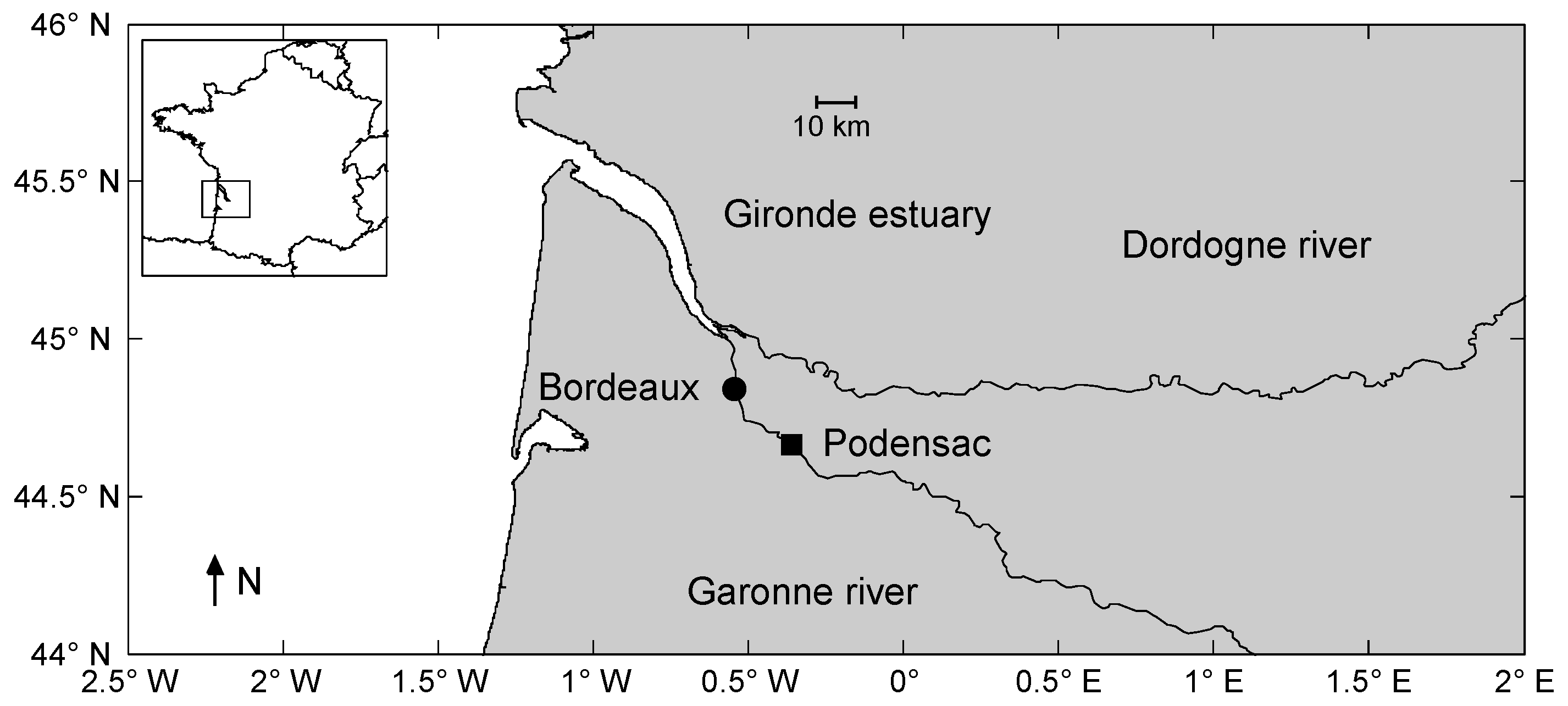
A 4-day experiment was conducted between the 16th and 19th of October 2016 on the Garonne River, at Podensac (see Figure 1). The Garonne River meets with the Dordogne River to form the Gironde estuary, where the so-called ’mascaret’ tidal bore forms [15]. This part of the Bay of Biscay coastline is a macrotidal environment with the tidal range at the field site in the range to m over the experiment period. Figure 2 shows the time-variation of the water depth over the whole experiment period, with the period of primary interest for this paper highlighted. For that particular tide (number 5), the Froude number was estimated to [5].
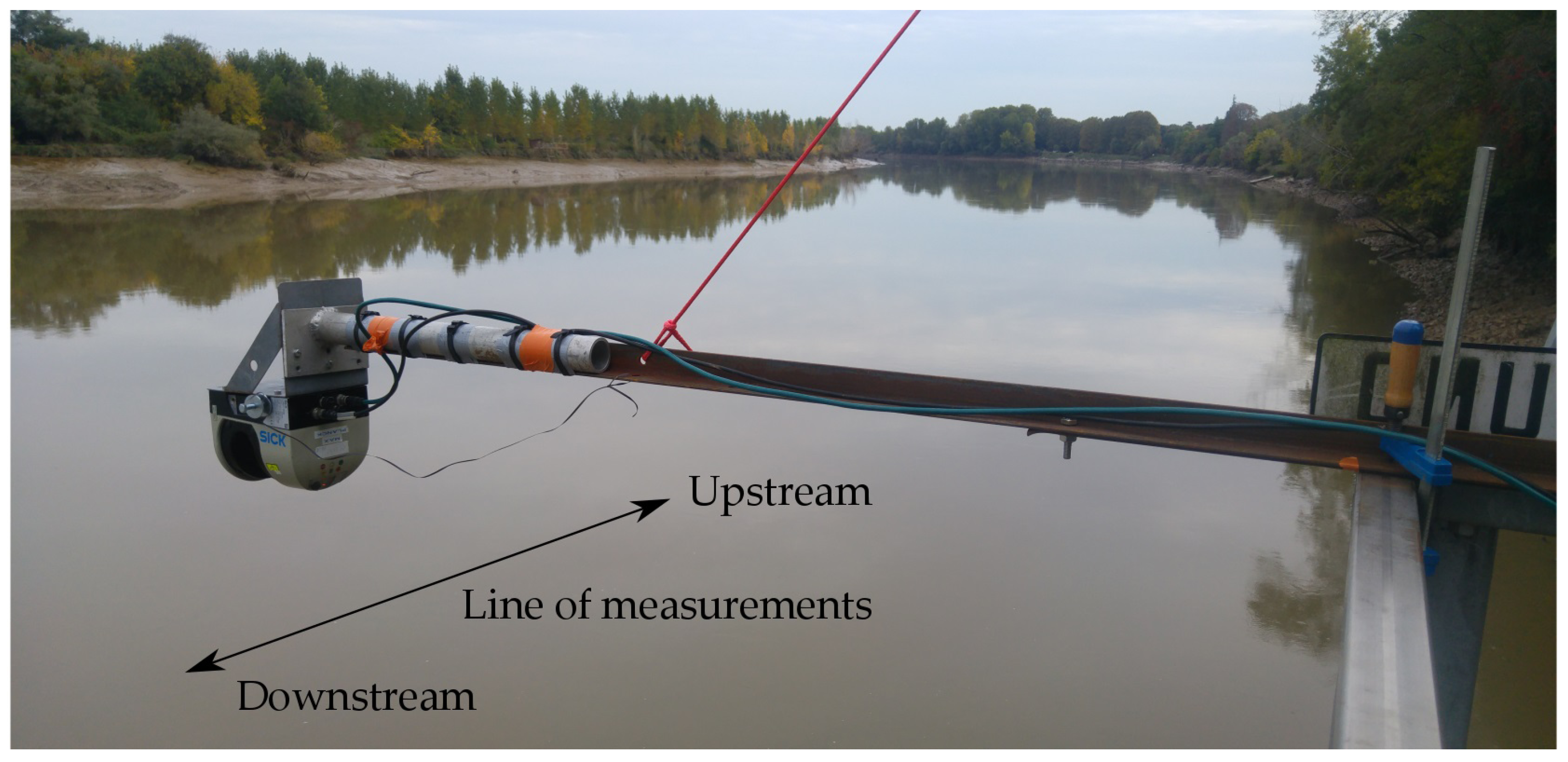
To measure the time-varying free surface during the passage of the tidal bore, a SICK LMS511 commercial 2D LiDAR scanner (SICK AG, Waldkirch, Germany) was cantilevered over the side of the field site platform (see Figure 3), extending m from the safety railing. The typical height of the scanner above the mean water level prior to the passage of the tidal bore was 8 m. A recent description of the working principle of the LiDAR can be found in [10]. A description of the 2D scanner used in the present study is provided in [9]. Data was collected at a sampling rate of Hz, with an angular resolution of 0.1667°. This corresponded to a spatial resolution during passage of the undular bores ranging from m at nadir to 0.05 m at the outer edges of the LiDAR scans.
On the same cross-section line as the LiDAR and at a distance of approximately 1.3 m from it, a Nortek Signature 1000 kHz current profiler (Nortek AS, Rud, Norway) was deployed together with a pressure transducer sampling at 10 Hz (Ocean Sensor Systems, Inc. Coral Springs, FL, USA). To reconstruct the time-varying surface elevation from the measured pressure signal, the hydrostatic relation has been used, as this provides the opportunity to study the non-hydrostatic nature of the mascaret:
where h is the water depth assuming hydrostatic pressure, p the measured pressure, the water density, g gravity and the atmospheric pressure. Additionally, an Optical Backscatter Sensor sampling at Hz (Campbell, Inc., Logan, UT 84321-1784, USA) was deployed to monitor the water turbidity at the bed. The Signature kHz also collects altimeter data using its vertical beam (hereafter referred to as the acoustic sensor, sampled at 8 Hz). Three different methods to detect the water surface location were therefore used and are compared in this paper: direct measurement by laser from the LiDAR, by an acoustic signal from the bottom-mounted Signature 1000 kHz and reconstructed from the pressure measurements at the bottom.
An undular bore is made up of a primary wave, i.e., a mean jump, between two different states of velocity and water depth, on which is superimposed secondary waves known as whelps when referring to a tidal bore. Bonneton, P. et al . [5,15] showed that the tidal bore mean jump is nearly uniform over the river cross section and that its intensity (or its Froude number) is mainly controlled by the local dimensionless tidal range , where is the tidal range and is the cross-sectionally averaged water depth. By contrast, a strong variability along the river cross section of the secondary wave field can be observed, with whelp amplitude generally larger at the banks than in the mid-channel [5,15]. This variability is due to the interaction between the secondary wave field and the gently sloping alluvial river banks. In the present paper, we analyse the non-breaking wave field close to the bank. Despite being relatively close to the river side, no breaking was observed below the LiDAR during the experiments.
2.2. Processing of the LiDAR Data
To track the tidal bore and its properties, the LiDAR measurements were first rotated to correct for the roll angle introduced at deployment. This was done by matching the data prior to the tidal bore passage to a horizontal free surface. The measurements are then interpolated onto a m regular along-stream grid. When carrying out this process, it was found that the mean free surface was slightly bent toward the edges of the scanning range (see Appendix A). The methodology of [13] to correct the bent edges was applied to a wave dataset by [16], but higher frequency waves seemed to be introduced in the surface elevation timeseries, showing that it might not be appropriate. As similar profile distortion was observed in the present study, some baseline measurements were performed on a solid horizontal surface with the same ranging distance to investigate this phenomenon for a case without the possibility of any signal penetration (see Appendix A). The results showed that the LiDAR profile curvature was entirely due to the deformation of the light beam on the surface for high incident angles, rather than signal penetration in the water column.
Based on these results, the free surface prior to the passage of the bore was extracted using the methodology described in the Appendix that uses the distinct peaks in elevation point distribution (corresponding to the ’real’ surface and sub-surface). Just after the passage of the tidal bore, no filter was applied to the measurements to correct for curvature or signal penetration. This is justified by the fact that the tidal bore mixes the water column [14], hence greatly increasing the turbidity and the surface roughness, which allows for more consistent detection of the ’real’ free surface. In fact, no rapid fluctuations in the surface timeseries were observed immediately after its passage (see Figure A1 for illustration). Note that the curvature only induces changes of m over a distance of m (1.5% of the first wave height), and does not affect the local wave properties (wave height H and celerity c).
3. Results
3.1. Comparison with In Situ Sensors
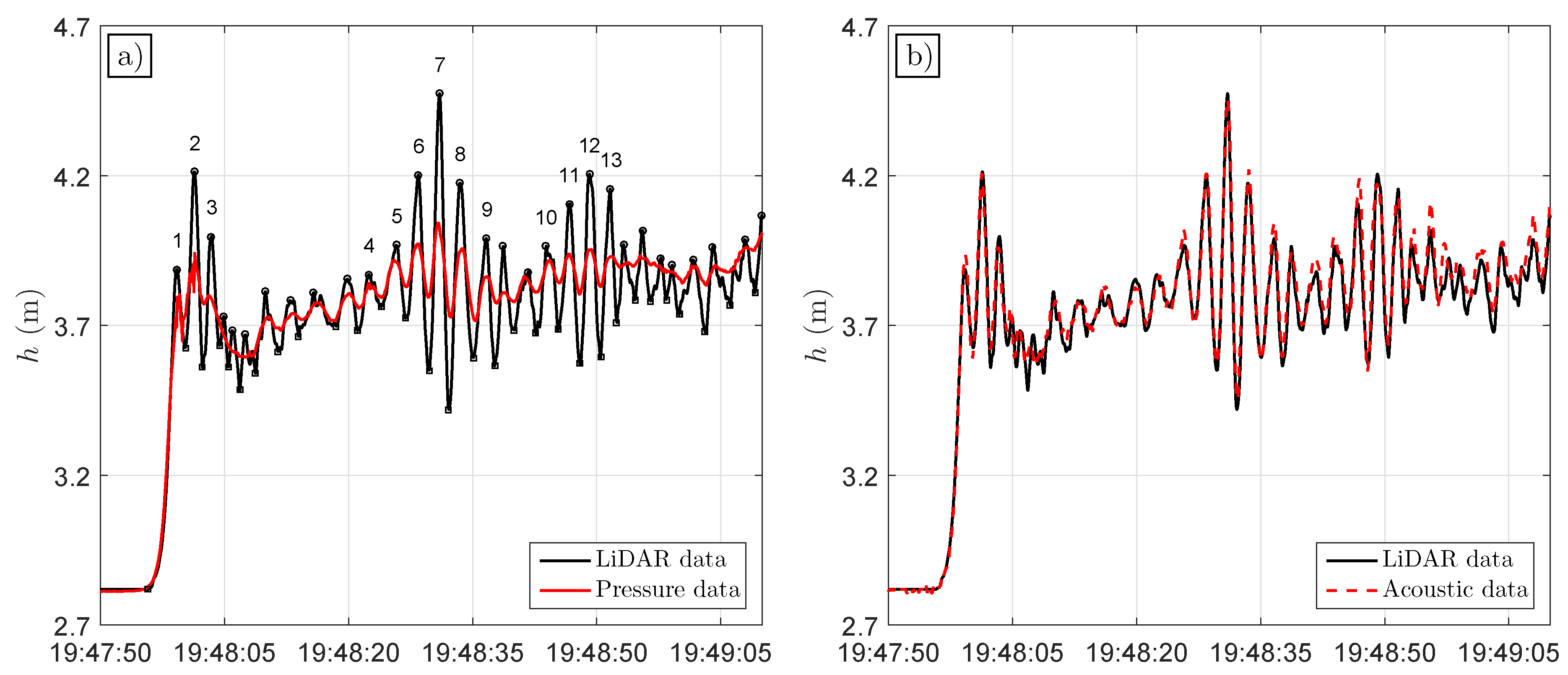
The water depth measured by the LiDAR scanner at the nadir was compared with the water depth derived from the pressure and acoustic sensors. Figure 4a shows the comparison with the pressure sensor and illustrates the non-hydrostatic nature of the tidal bore secondary wave field. The discussion here focuses on tide number 5 (see Figure 2), which provided the best LiDAR dataset: high tidal coefficient and low humidity, which minimizes signal losses. Indeed, due to the transient nature of the tidal bore and the innovative character of the experiments, the preceding tides were used to optimize the data collection process for tide 5. For instance, the early morning tides did not allow for the collection of usable data, due to strong fog conditions. It is worth noting that the present dataset was obtained without any atmospheric filter in the data collection software (SOPAS Engineering Tool©, SICK AG).
It is observed in Figure 4a that, except for the mean jump of the tidal bore, the signal reconstructed from the pressure using the hydrostatic assumption largely underestimates the wave amplitudes, regardless of their characteristics (wave height or wave length). For this comparison, a Root mean square error () of m is obtained, with a correlation coefficient and scatter index () of 0.03. By contrast, the agreement between acoustic-derived water depth and the LiDAR data, which both directly measure the time-varying water surface elevation is very good ( m, and ) (see Figure 4b). Despite the increasing turbidity levels as the tidal bore propagates, the surface is still accurately detected by the bottom-mounted sensor. A slight overestimation of the water depth measured by the acoustic sensor seems to occur after the second wave group passage. As the two measurements (LiDAR and acoustic) give very similar results far behind the bore front, this is mainly explained by an underestimation of the acoustic wave celerity when the turbidity is at its maximum in the water column, just a few minutes after the bore passage [14].
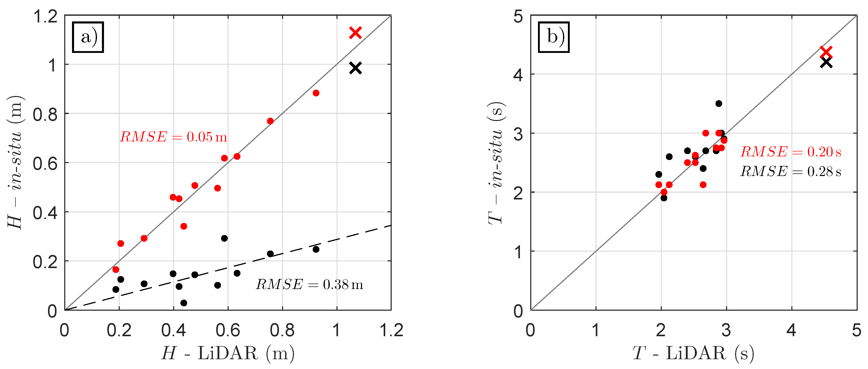
To further illustrate the non-hydrostatic nature of the bores, a wave-by-wave analysis was performed on the three datasets: individual waves were extracted by detecting wave crests and surrounding troughs [9]. The wave height H is defined as the vertical distance between crest and preceding trough while the wave period is defined as the time elapsed between the passages of the two surrounding troughs at the nadir of the LiDAR measurements. Figure 5 shows the comparison of H and T extracted from the three datasets for the thirteen waves numbered in Figure 4a. It is observed that differences up to m (75% of H) exist for the 6th wave between the pressure-derived and LiDAR datasets. Only small discrepancies (error of 8% of H) are observed for the primary wave front height. This is thought to be because the first wave front is effectively a surge where the mean water level suddenly increases and so is mostly captured using a hydrostatic assumption; however, this approach is unable to capture the more rapid surface fluctuations in the secondary wave field. Better agreement is found for H between the acoustic-derived and LiDAR datasets ( of m against m for the pressure data, see Figure 5). Similarly, a better fit between acoustic and LiDAR datasets than between pressure-derived and LiDAR is observed for the wave periods. This is mainly explained by the flatter troughs in the hydrostatic signal, which can delay the detection of the minimum, defining the wave trough. The relatively good fit between pressure-derived and LiDAR wave periods suggest that the pressure peaks at the river bottom coincide to those at the free surface.
3.2. Spatial Structure of the Tidal Bore
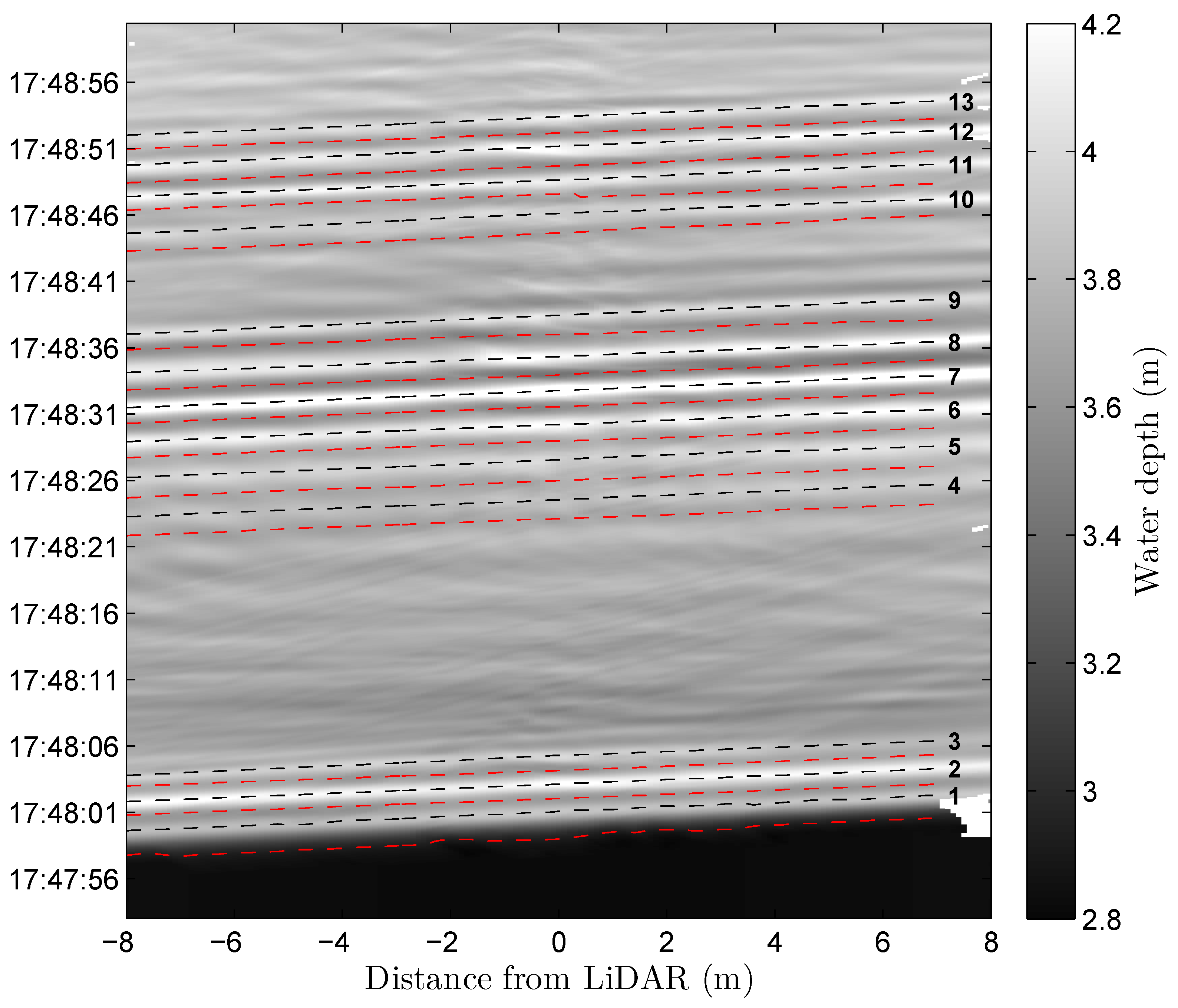
Individual waves and their properties were tracked using the wave-by-wave approach described in [12]. The methodology described in Section 3.1 to extract wave crests can be applied at different along stream positions, which enables the tracking of a wave and its properties in time and space. At every position of the 0.1 m regular grid, the wave crests were detected in the surface elevation timeseries using this procedure, allowing geometrical properties such as wave height H and wave period T to be studied in the direction of propagation (along-stream direction). Figure 6 displays the obtained wave tracks on a timestack of surface elevation profiles measured by the LiDAR. Because the spatial information of the waves is available at the same time as the temporal characteristics, the wave celerity can also be directly estimated. Table 1 presents the averaged individual wave properties and the standard deviation for every wave tracked in Figure 6. An interesting observation lies in the steep front observed in the highest wave of the first group (number 7). In the present conditions, this wave is actually steeper than the bore front, and this may explain why breaking sometimes occurs behind the tidal bore, while the front is not breaking.
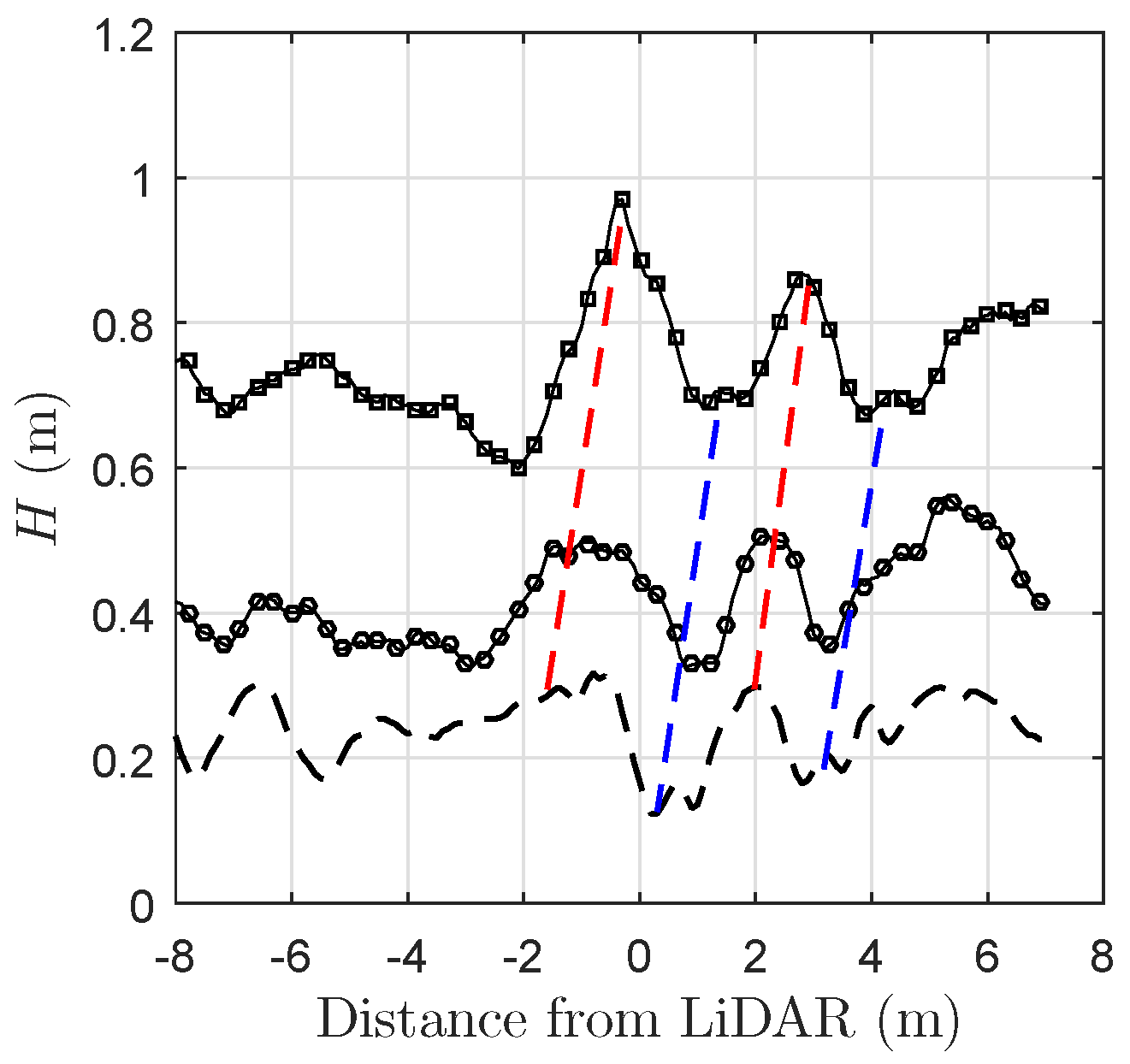
Figure 7 shows the evolving shape of the tidal bore front and the following wave (1 and 2 in Figure 4a). The tidal front wave is found to steepen just in front of the LiDAR platform (Figure 6a); this process is accompanied by a slight increase of the wave height (Figure 7b) and a decrease in local wave celerity (not shown). This is likely to be due to a shoaling effect caused by decreasing water depth under the platform, as measured by depth soundings obtained around the platform. The second wave is affected by the presence of a scattered wave, probably generated from the first wave either from the platform or from the river banks (reflection), which locally affects both the wave steepness and the wave height. When the crest of the scattered wave interferes with the crest of the second wave, the local wave height is enhanced (see at nadir, Figure 7b,d and when the scattered wave trough interferes with the crest, H decreases locally. This appears in the local wave steepness (Figure 7a) as rapid fluctuations of the order of 2–2.5°. This phenomenon is of the same nature as observed in [12], where it was shown that reflected waves caused intra-wave variability of individual wave properties in the surf zone of a prototype-scale laboratory beach. The wave profile evolution displayed in Figure 7d further illustrates this process of interaction with the steeper, larger wave detected around the nadir. In contrast, the tidal bore front wave shape is more stable (Figure 7c).
This interaction between scattered waves and whelps is also observable in the individual properties of the secondary waves. Figure 8 shows the along-stream evolution of the individual wave height from tracked waves numbers 5, 6 and 7 (Figure 4a). Since the waves are increasing in size, the paths of scattered wave crests and troughs are clearly observed. These interactions can also be seen in the timestack of Figure 6 with local fluctuations of the surface elevation. They have the effect of making the individual wave height and period fluctuate due to the propagation of scattered wave crests and troughs (Table 1).
4. Discussion
A tidal bore is a highly nonlinear wave accompanied by secondary waves that cannot be studied using the assumption of a hydrostatic pressure distribution (Figure 4a and Figure 5a). Depth attenuation of the pressure signal is typically corrected in datasets from coastal environments such as the surf zone (see e.g., [17]). In practice, the correction derived from linear theory is applied to each frequency of the surface elevation Fourier spectrum (denoted by ):
with the surface elevation around a mean derived with the hydrostatic assumption (Equation (1)). represents the transfer function applied for the frequency f and is defined as follows:
where is the height of the pressure sensor above the bed, the wavenumber associated to the frequency f and the mean water depth. As this relation needs the description of the surface elevation around a mean state, this formulation is not fully adapted to a tidal bore that is characterized by a mean jump. Another approach remains possible and consists of directly correcting the individual wave height from the pressure-derived dataset (Figure 5a) using the wavenumber estimated from the LiDAR scanner:
where is the transfer function for the measured individual wave defined as follows:
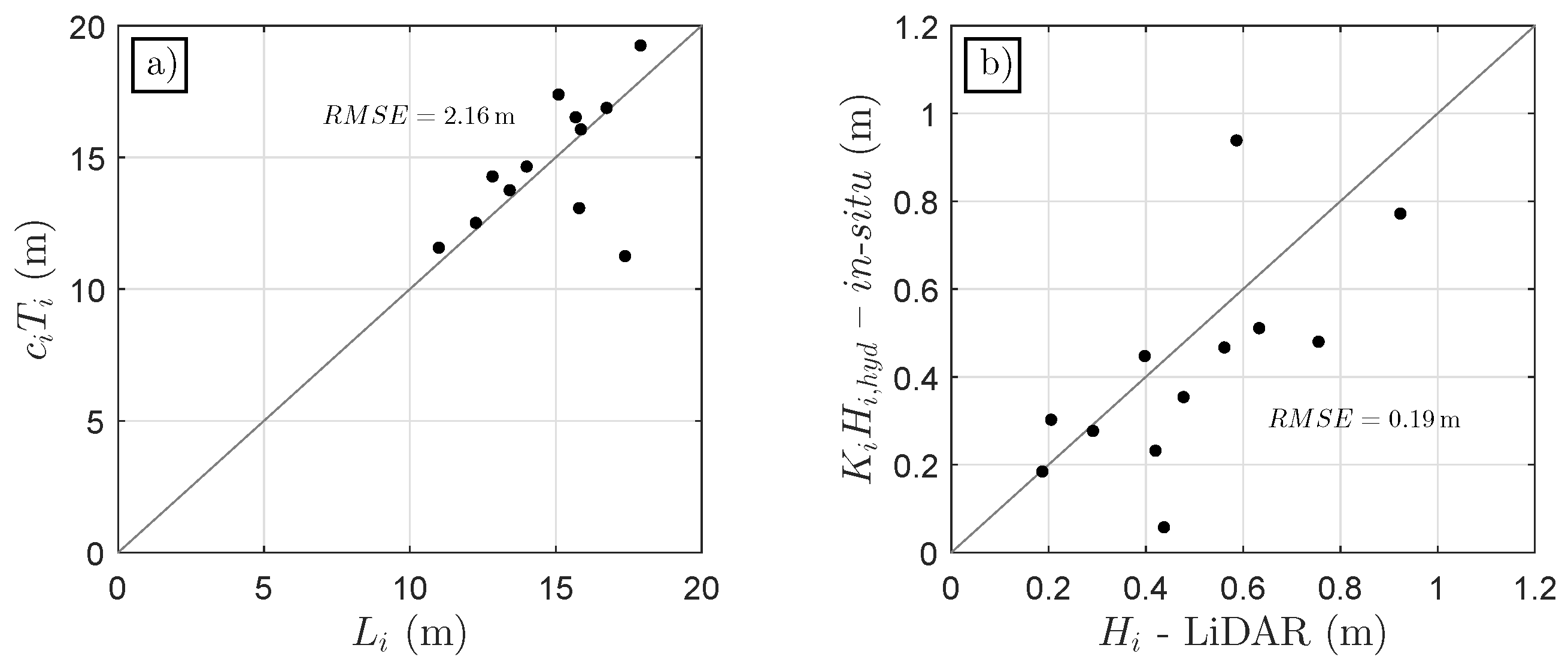
Equation (5) requires an estimate of an individual wavelength , which can be obtained by evaluating . The drawback of this method lies in the nonlinearity and unsteadiness of an individual wave: as shown before, can vary over small distances and can be influenced by the presence of scattered waves. When LiDAR data is available, the wavelength can be estimated directly, as the whole wave is visible when the crest is around the nadir. Figure 9a shows the comparison between measured wavelength (distance between two surrounding troughs) and . It is observed that generally overestimates the ’instantaneous’ wavelength directly estimated from the LiDAR but generally provides a good estimate. The comparison between corrected wave heights and measured wave heights by the LiDAR are shown in Figure 9b. Except for wave number 2 (see Figure 4a), the depth attenuation based on linear wave theory is able to reconstruct the wave height measured using the LiDAR ( of m against m without correction).
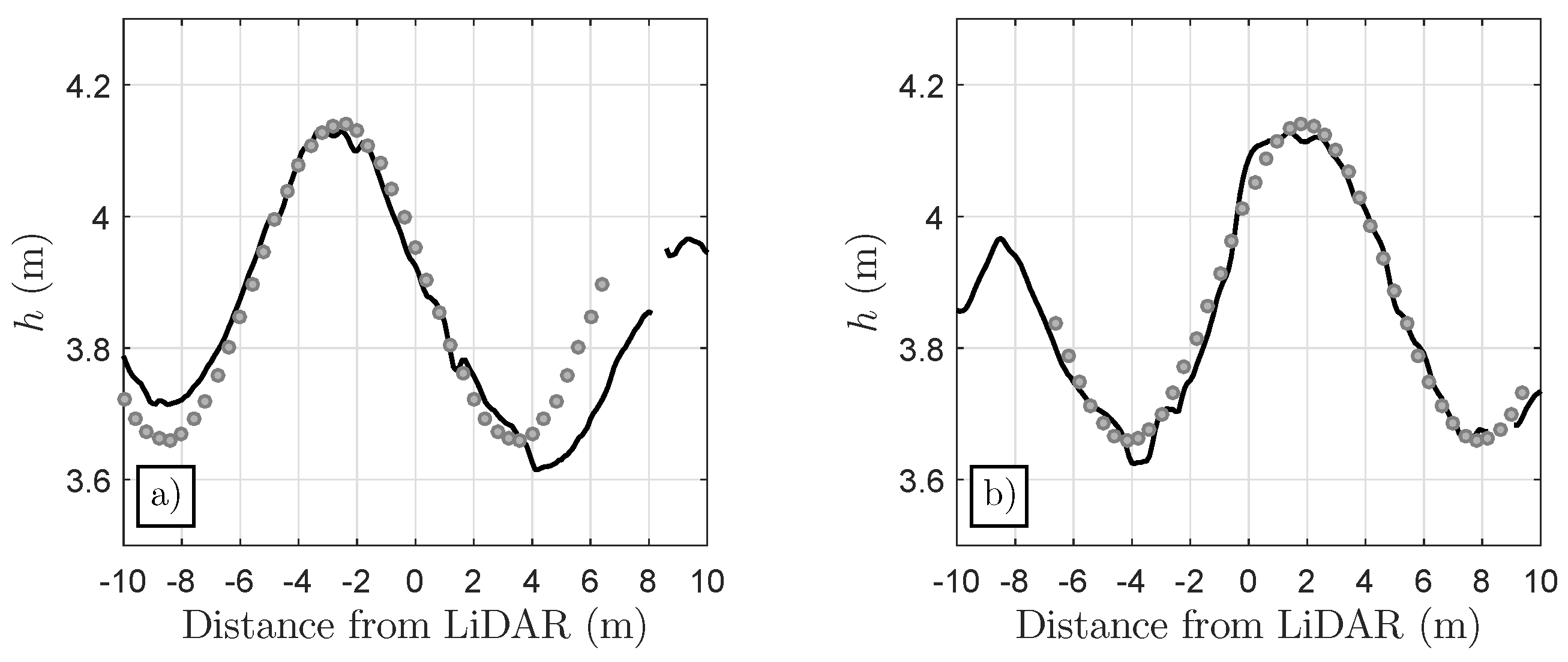
This is an interesting result as it would be expected that nonlinear effects could have an impact on the wave geometry, due to the nonlinear character of the tidal bore, but also to the interactions with the low-sloping estuarine banks [5]. Chanson, H. et al. [18] tried to fit wave profiles from linear wave and Boussinesq theory to measurements. Some discrepancies were observed in the wave shape, and especially its asymmetry. Similar comparisons were performed here and an example is displayed in Figure 10 for the tracked wave number 2. The linear wave profile was constructed using the mean individual wave properties presented in Table 1. While the comparisons in Figure 10a exhibit some clear discrepancies, especially in the asymmetric surrounding trough positions, the two profiles match very well at the later stage of the propagation (Figure 10b). The primary reason for this is the effect of the interactions discussed earlier (Figure 6, Figure 7 and Figure 8) between scattered waves and the secondary wave field. We can therefore hypothesize that, despite the nonlinear character of the tidal bore, the individual waves in the secondary wave field have a general form close to that described by linear wave theory. However, the presence of scattered waves can induce some asymmetry in the crest/trough locations and the wave steepness, inducing potential discrepancies with commonly used wave theory. Additionally, these interactions might, in turn, trigger some breaking events.
5. Conclusions
A 2D commercial LiDAR scanner has been deployed for the first time to monitor the undular tidal bore of the Garonne River, at high spatial and temporal resolution. The procedure to extract the water level prior to the passage of the bore has been described. This analysis showed that the bent edges of the scanning profiles previously observed with the scanner model for low incident angle are actually due to the displacement of the highest return point, when the light beam goes from a circle to an ellipse for high incident angles, and not to the signal penetration in the water column.
For this Froude number, it was shown that the pressure under the mean jump accompanying the tidal bore is approximately hydrostatic. However, the hydrostatic hypothesis is inadequate for reconstructing the secondary wave field: large differences are observed at the wave-by-wave scale, especially for the wave height ( of m over 13 waves). Despite the high levels of turbidity encountered, the acoustic sensor performed extremely well and was able to measure the individual wave characteristics accurately ( m). The results show that LiDAR technology can be used to obtain accurate measurements of undular tidal bore geometry, even in the absence of breaking events, which greatly contributes to the advancement of coastal ocean and riverine observing systems [19]. Here, the field deployment focused on the along-stream direction; the analysis highlighted the influence of scattered wave on individual wave properties and profile. However, the possibility of deploying a 2D LiDAR scanning in the cross-section direction seems very promising and could elucidate the variability of the secondary wave field along the cross-section direction.
Acknowledgments
The authors would like to acknowledge the financial assistance provided by Centre National d’Études Spatiales (CNES) through the Terre, Océan, Surfaces continentales, Atmosphère) (TOSCA) grant Global Navigation Satellite Systems (GNSS)-R Appliqué à l’Environnement Littoral (GRAEL). Kévin Martins was supported by the University of Bath, through a University Research Services (URS) scholarship. The assistance of G.s.m in facilitating access to the site platform is greatly appreciated. Finally, the three reviewers are greatly acknowledged for their constructive comments, which helped improving the manuscript.
Author Contributions
Kévin Martins deployed the LiDAR scanner with the assistance of Guillaume Detandt, did all the analysis related to the LiDAR scanner, and wrote the article. Philippe Bonneton, Natalie Bonneton and Frédéric Frappart designed the experiment and post-processed the in situ data from the sensors that Guillaume Detandt deployed. Chris Blenkinsopp and Philippe Bonneton supervised the analysis performed on the whelps and greatly contributed to the manuscript.
Conflicts of Interest
The authors declare no conflict of interest. The founding sponsors had no role in the design of the study; in the collection, analyses, or interpretation of data; in the writing of the manuscript, and in the decision to publish the results.
Appendix A. Accurate Detection of Steady Water Surface with a 2D LiDAR Scanner
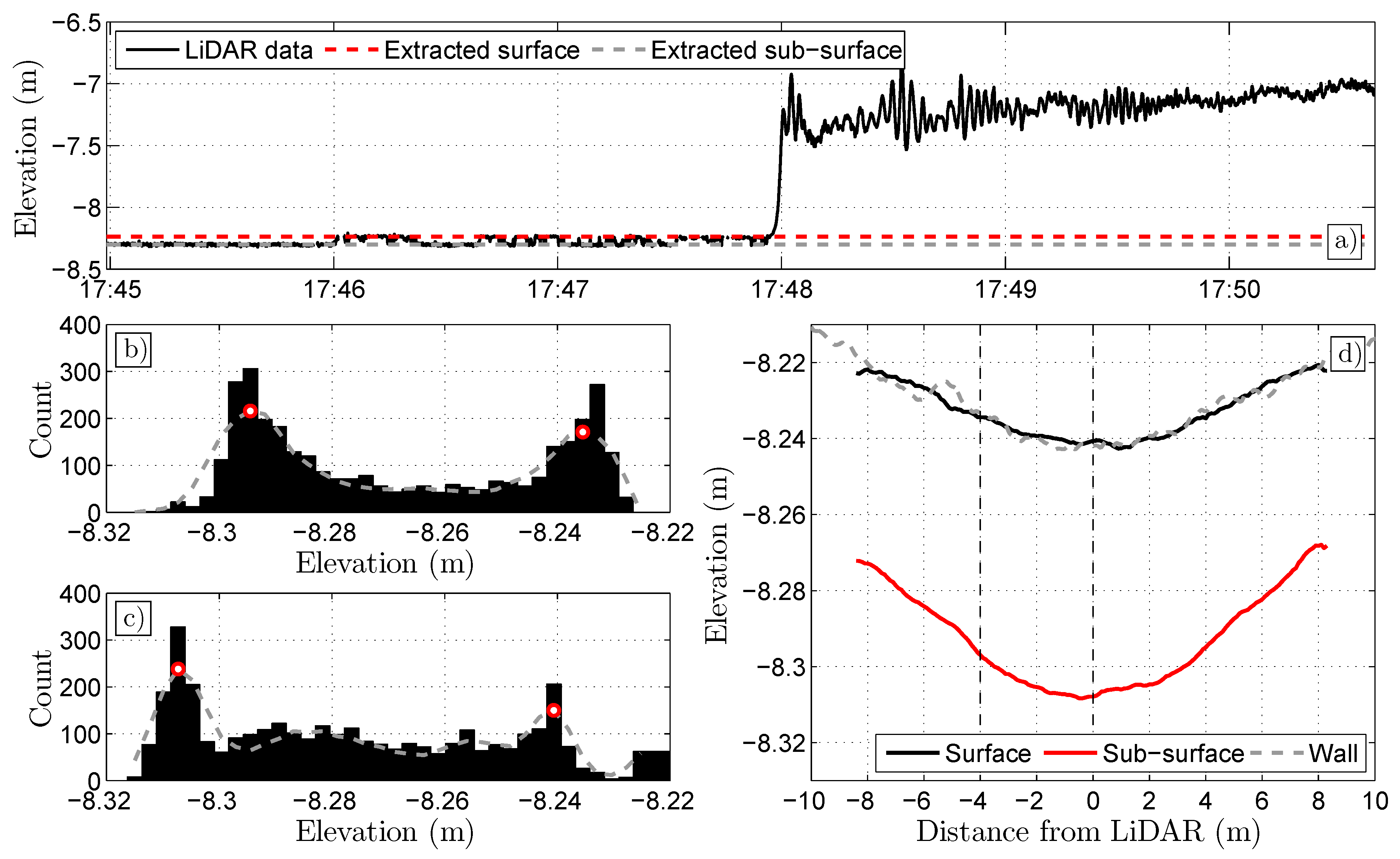
As the Garonne River is naturally turbid, the scanner beam may be reflected by the ’real’ free surface, or by particles in suspension at some depth below the surface (this is referred to as sub-surface hereafter). An example of this is shown at nadir in Figure A1a prior to the arrival of the bore front at 17:48. The elevation obtained from the LiDAR is observed to jump between two elevations approximately 0.06–0.07 m apart. If it is assumed that the real surface will always lie above the sub-surface, the correct elevation of the flat water surface prior to the passage of the mascaret can be resolved.
At each LiDAR measurement position, the distribution of the measured elevations LiDAR was computed (two examples shown in Figure A1b,c). Because the measurements typically oscillate between the real and sub-surface, the elevation distribution features two distinct peaks. The correct elevation of the real and sub-surface were estimated by detecting these two peaks. This process was performed at every measurement location and the resulting measured ’flat’ real and sub-surfaces are shown in Figure A1d.
To explain the bent edges of the measured surface profiles (see also in [13]) the surface of a wall at the same distance range was measured. This represents a ’no-penetration’ test, the results of which are also shown in Figure A1d. It is observed that the real free surface has the same curvature as the wall, which gives confidence to the method to separate the two surfaces. This result also suggests that the penetration of the signal observed with the same LiDAR scanner in previous studies was not the reason for the water surface curvature, as suspected by [13]. As the incident angle increases, the beam projection becomes an ellipse (see Figure A2) and we hypothesize that the energy spreads in this increased surface area [20]. The scanner then matches the strongest reflected signal to the theoretical position, located at the centre of the ellipse. However, in practice, the position of the strongest reflected signal moves away from the beam centre, as illustrated in Figure A2. This means that the distance measured is shorter than for the assumed measurement location. At high incident angle, this has the effect of introducing curvature into the measured surfaces.
The sub-surface has a slightly different curvature, due to the fact that closer to the nadir, the signal penetrates deeper into the water column since it is stronger for lower incident angle. The penetration extent ranges from m around the nadir to m at the outer edges of the LiDAR scans. Attempts to correct for the observed profile curvature were not performed for this study as the effect was considered negligible: the changes are small compared to the height of the bore front, and, after its passage, the turbidity and surface roughness significantly increase, which ensured that the scanner detected the real surface.
Finally, it is worth noting that the LiDAR scanners provide an output of the return signal strength index (RSSI). The RSSI was not found to vary significantly between no-penetration/penetrating cases, at a fixed along-stream position. In fact, for the present dataset (Tide 5), it was found to linearly increase from the downstream to upstream direction; the light conditions (nightfall in this case) are suspected to have influenced this quantity.
Figure A1.
Illustration of the methodology developed to extract the free surface elevation prior to the bore passage. (a) shows the surface elevation timeseries measured by the LiDAR scanner at the Nadir ( m); (b,c) show the distribution of the elevation points measured at and 0 m, respectively. The window-averaged distribution is shown as a dashed grey line. The two peaks, corresponding to the average position of the surface and sub-surface, are represented using red circles. (d) shows the curved real and sub-surface elevations extracted using the distribution peak methodology. Measurements of a horizontal wall at the same range as measured in the field are also provided. Note that the vertical, z datum is given relative to the LiDAR scanner (and not to the river bed).

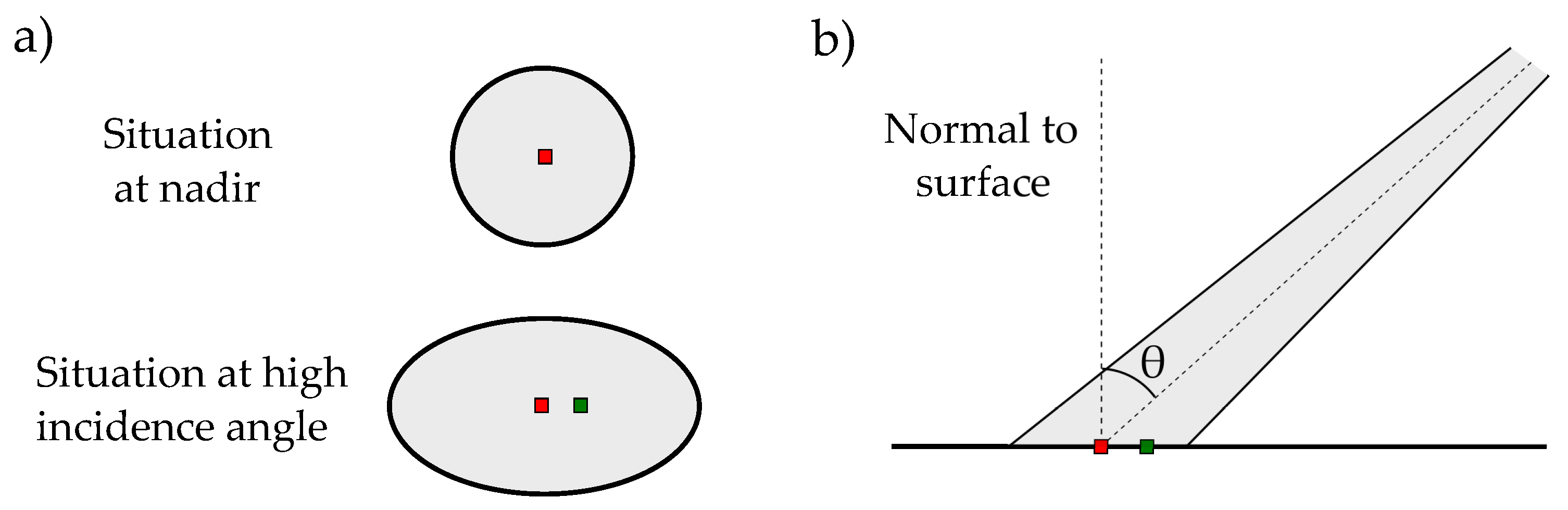
Figure A2.
Schematic of the LiDAR beam spot deformation at high incident angle : (a) shows a view from above the surface measured by the scanner; (b) shows the lateral view. The red squares represent the centre of the LiDAR beam, which is generally assumed to be the measurement location. The green squares represent the actual measurement location. Note that, at the nadir, these are the same.

References
- Bonneton, P.; Filippini, A.G.; Arpaia, L.; Bonneton, N.; Ricchiuto, M. Conditions for tidal bore formation in convergent alluvial estuaries. Estuar. Coast. Shelf Sci. 2016, 172, 121–127. [Google Scholar] [CrossRef]
- Madsen, P.A.; Fuhrman, D.R.; Schäffer, H.A. On the solitary wave paradigm for tsunamis. J. Geophys. Res. Oceans 2008, 113. [Google Scholar] [CrossRef]
- Tissier, M.; Bonneton, P.; Marche, F.; Chazel, F.; Lannes, D. Nearshore dynamics of tsunami-like undular bores using a fully nonlinear Boussinesq model. J. Coast. Res. 2011, 64, 603. [Google Scholar]
- Vignoli, G.; Toffolon, M.; Tubino, M. Non-linear frictional residual effects on tide propagation. In Proceedings of the XXX IAHR Congress, Thessaloniki, Greece, 1–31 August 2003. [Google Scholar]
- Bonneton, P.; Bonneton, N.; Parisot, J.-P.; Castelle, B. Tidal bore dynamics in funnel-shaped estuaries. J. Geophys. Res. Oceans 2015, 120, 923–941. [Google Scholar] [CrossRef]
- Frappart, F.; Roussel, N.; Darrozes, J.; Bonneton, P.; Bonneton, N.; Detandt, G.; Perosanz, F.; Loyer, S. High rate GNSS measurements for detecting non-hydrostatic surface wave. Application to tidal bore in the Garonne River. Eur. J. Remote Sens. 2016, 49, 917–932. [Google Scholar] [CrossRef]
- Blenkinsopp, C.E.; Mole, M.A.; Turner, I.L.; Peirson, W.L. Measurements of the time-varying free-surface profile across the swash zone obtained using an industrial (LIDAR). Coast. Eng. 2010, 57, 1059–1065. [Google Scholar] [CrossRef]
- Brodie, K.L.; Raubenheimer, B.; Elgar, S.; Slocum, R.K.; McNinch, J.E. Lidar and Pressure Measurements of Inner-Surfzone Waves and Setup. J. Geophys. Res. Oceans 2015, 32, 1945–1959. [Google Scholar] [CrossRef]
- Martins, K.; Blenkinsopp, C.E.; Zang, J. Monitoring Individual Wave Characteristics in the Inner Surf with a 2-Dimensional Laser Scanner (LiDAR). J. Sens. 2016, 1–11. [Google Scholar] [CrossRef]
- Tamari, S.; Guerrero-Meza, V. Flash Flood Monitoring with an Inclined Lidar Installed at a River Bank: Proof of Concept. Remote Sens. 2016, 8. [Google Scholar] [CrossRef]
- Tamari, S.; Guerrero-Meza, V.; Rifad, Y.; Bravo-Inclán, L.; Sánchez-Chávez, J.J. Stage Monitoring in Turbid Reservoirs with an Inclined Terrestrial Near-Infrared Lidar. Remote Sens. 2016, 8. [Google Scholar] [CrossRef]
- Martins, K.; Blenkinsopp, C.E.; Almar, R.; Zang, J. The influence of swash-based reflection on surf zone hydrodynamics: A wave-by-wave approach. Coast. Eng. 2017, 122, 27–43. [Google Scholar] [CrossRef]
- Streicher, M.; Hofland, B.; Lindenbergh, R.C. Laser Ranging For Monitoring Water Waves in the New Deltares Delta Flume. ISPRS Ann. Photogramm. Remote Sens. Spat. Inf. Sci. 2013, 2, 271–276. [Google Scholar] [CrossRef]
- Tessier, B.; Furgerot, L.; Mouazé, D. Sedimentary signatures of tidal bores: A brief synthesis. Geo-Mar. Lett. 2016, 1–7. [Google Scholar] [CrossRef]
- Bonneton, P.; Parisot, J.-P.; Bonneton, N.; Sottolichio, A.; Castelle, B.; Marieu, V.; Pochon, N.; van de Loock, J. Large Amplitude Undular Tidal Bore Propagation in the Garonne River, France. In Proceedings of the Twenty-First (2011) International Offshore and Polar Engineering Conference, Maui, HI, USA, 19–24 June 2011. [Google Scholar]
- Damiani, L.; Valentini, N. Terrestrial Laser Scanner as a measurement instrument for laboratory water waves. In SCORE@ POLIBA 2014; Cangemi Editore SPA: Roma, Italy, 2014; pp. 63–67. [Google Scholar]
- Bishop, C.T.; Donelan, M.A. Measuring waves with pressure transducers. Coast. Eng. 1987, 11, 309–328. [Google Scholar] [CrossRef]
- Chanson, H. Undular Tidal Bores: Basic Theory and Free-Surface Characteristics. J. Hydraul. Eng. 2011, 136, 940–944. [Google Scholar] [CrossRef]
- Liu, Y.; Kerkering, H.; Weisberg, R.H. Coastal Ocean Observing Systems; Elsevier (Academic Press): London, UK, 2015. [Google Scholar]
- Soudarissanane, S.; Lindenbergh, R.; Menenti, M.; Teunissen, P. Incidence angle influence on the quality of terrestrial laser scanning points. In Laser Scanning 2009; Bretar, F., Pierrot-Deseilligny, M., Vosselman, G., Eds.; International Society for Photogrammetry and Remote Sensing: Paris, France, 2009; Volume XXXVIII, pp. 183–188. [Google Scholar]
Figure 1.
Location map of the Gironde estuary in the Bay of Biscay. The field site of Podensac is shown as a black square.
Figure 1.
Location map of the Gironde estuary in the Bay of Biscay. The field site of Podensac is shown as a black square.

Figure 2.
Water depth evolution over the course of the experiments. The water depth was derived from the pressure measurements assuming hydrostatic pressure (Equation (1)). The present paper uses mainly data from the tide monitored number 5, which is highlighted by the grey region.
Figure 2.
Water depth evolution over the course of the experiments. The water depth was derived from the pressure measurements assuming hydrostatic pressure (Equation (1)). The present paper uses mainly data from the tide monitored number 5, which is highlighted by the grey region.
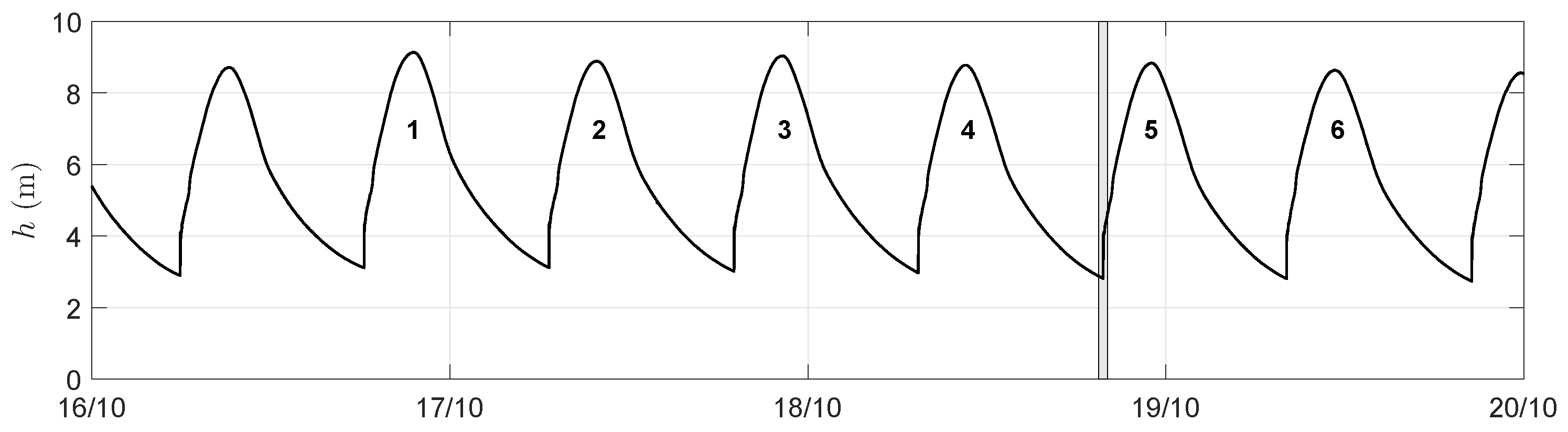
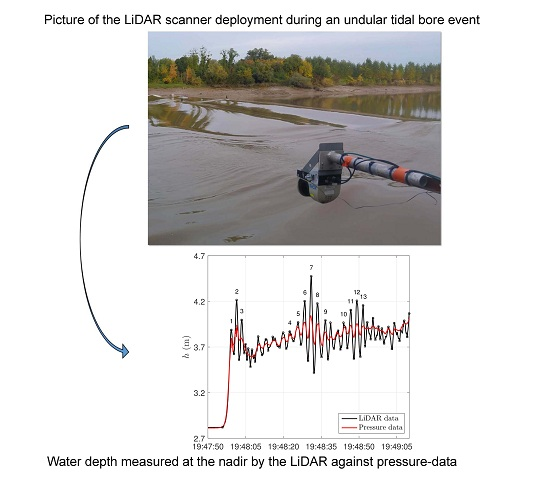
Figure 3.
Photograph of the LiDAR scanner deployment. The scanner was cantilevered over the platform edge, at a distance of approximately m. The scanning line was approximately m from the river bank at low tide.
Figure 3.
Photograph of the LiDAR scanner deployment. The scanner was cantilevered over the platform edge, at a distance of approximately m. The scanning line was approximately m from the river bank at low tide.

Figure 4.
Comparison of the measured water depths by the pressure, acoustic and LiDAR sensors at the nadir. (a) shows the pressure-derived water depth timeseries computed with the hydrostatic assumption (Equation (1)) from pressure data along with the LiDAR data for the tide number 5 (grey shaded region in panel Figure 3); (b) compares the acoustic-derived water depth with the LiDAR data for the same time period.

Figure 5.
Comparison of the 13 individual wave properties extracted from the LiDAR (Figure 3a) with in situ pressure-derived data (black dots) and acoustic sensor data (red dots). The root-mean square errors between the datasets are directly shown in the plots, in the corresponding colour; (a) shows the individual wave height H. For indication, the linear regression fit forced to pass in (0,0) performed on the secondary waves is shown for the pressure-derived data (slope of 0.28). (b) shows in the individual wave period T. The bore front properties are shown as a cross. The 1:1 lines are shown as gray line.

Figure 6.
Timestack of the water depth measured by the LiDAR scanner during the tide number 5 (grey region in Figure 3). The individual wave crest and trough tracks are shown as black and red dashed lines, respectively. The same numbering as in Figure 4 is shown.

Figure 7.
Spatial evolution of waves numbers 1 and 2 (see Figure 4). (a,b) show the wave front angle and height, respectively, for wave 1 (black continuous line) and wave 2 (black dashed line); (c,d) show the wave propagation of waves 1 and 2, respectively: the wave profile is shown when the crest is detected at m intervals. For clarity, each profile is drawn in a different colour: wave profiles are first shown as thick red lines (first profile shown as thick red lines) and evolve towards black at the nadir, and finally blue after having passed under the LiDAR. Note that the tidal bore propagates from left to right (axis positive in the upstream direction).
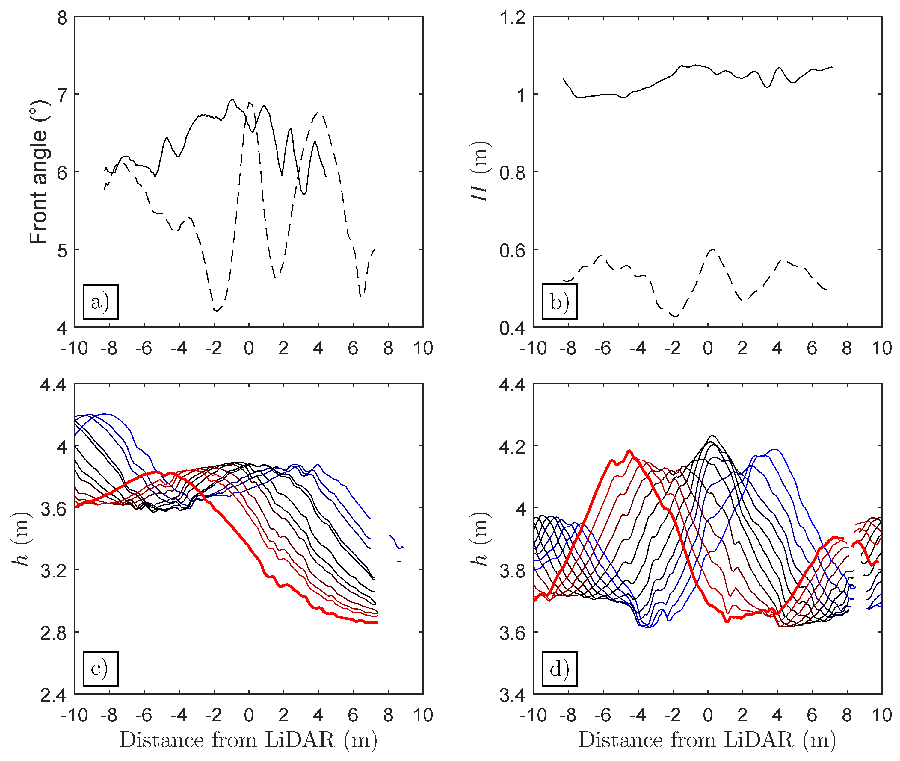
Figure 8.
Along-stream evolution of the individual wave height of wave numbers 5 (dashed black line), 6 (black line and circles) and 7 (black line and squares); see Figure 4a for wave numbering. The crest and trough paths of two scattered waves are shown as red and blue dashed lines, respectively.
Figure 8.
Along-stream evolution of the individual wave height of wave numbers 5 (dashed black line), 6 (black line and circles) and 7 (black line and squares); see Figure 4a for wave numbering. The crest and trough paths of two scattered waves are shown as red and blue dashed lines, respectively.

Figure 9.
Wave-by-wave depth attenuation correction of the pressure-derived wave heights. (a) shows the estimated individual wavelength as a function of the measured wavelength L estimated from the tracking algorithm (Section 4). In (b), the individual wave heights estimated from pressure measurements and corrected for depth attenuation are shown as a function of the wave height measured by the LiDAR. The 1:1 lines are shown by the gray line.

Figure 10.
Wave profile comparison between measurements (black line) and linear wave theory (gray dots) for wave number two (see Figure 4 or Figure 6), at two times: (a) when the wave crest is located at m; and (b) s after.

Table 1.
Mean () and standard deviation () values of every tracked individual wave from Figure 4a (see also Figure 6). The wavelength L is only estimated for wave crests located in the region to 2 m, since the wave trough can sometimes be out of the monitored area otherwise.
| Properties | 1 | 2 | 3 | 4 | 5 | 6 | 7 | 8 | 9 | 10 | 11 | 12 | 13 |
|---|---|---|---|---|---|---|---|---|---|---|---|---|---|
| (m/s) | 5.62 | 6.07 | 5.84 | 6.27 | 6.22 | 6.17 | 6.18 | 6.37 | 5.76 | 5.75 | 6.11 | 5.76 | 5.74 |
| (m/s) | 0.33 | 0.10 | 0.48 | 0.32 | 0.82 | 0.12 | 0.04 | 0.08 | 0.15 | 0.62 | 0.41 | 0.17 | 0.19 |
| (m) | 1.04 | 0.52 | 0.22 | 0.17 | 0.24 | 0.42 | 0.74 | 0.62 | 0.42 | 0.27 | 0.40 | 0.49 | 0.36 |
| (m) | 0.03 | 0.05 | 0.09 | 0.04 | 0.05 | 0.06 | 0.08 | 0.11 | 0.06 | 0.06 | 0.05 | 0.07 | 0.10 |
| (s) | 2.90 | 2.15 | 2.51 | 2.86 | 2.96 | 2.61 | 2.43 | 3.06 | 2.39 | 2.80 | 2.25 | 2.47 | 2.08 |
| (s) | 0.24 | 0.03 | 0.47 | 0.03 | 0.04 | 0.03 | 0.04 | 0.07 | 0.07 | 0.29 | 0.18 | 0.05 | 0.06 |
| (°) | 6.37 | 5.54 | 2.85 | 1.21 | 1.51 | 3.39 | 7.57 | 5.80 | 3.83 | 2.01 | 4.01 | 3.73 | 3.66 |
| (°) | 0.35 | 0.75 | 1.41 | 0.41 | 0.49 | 0.92 | 1.37 | 1.93 | 1.37 | 1.93 | 0.95 | 0.84 | 1.01 |
| (m) | - | 12.3 | 17.9 | 16.6 | 16.8 | 15.3 | 14.2 | 17.4 | 13.1 | 15.4 | 16.5 | 12.8 | 10.8 |
| (m) | - | 0.78 | 0.83 | 1.20 | 0.88 | 1.27 | 0.49 | 0.76 | 1.68 | 0.04 | 1.53 | 0.38 | 0.58 |
© 2017 by the authors. Licensee MDPI, Basel, Switzerland. This article is an open access article distributed under the terms and conditions of the Creative Commons Attribution (CC BY) license (http://creativecommons.org/licenses/by/4.0/).
Share and Cite
MDPI and ACS Style
Martins, K.; Bonneton, P.; Frappart, F.; Detandt, G.; Bonneton, N.; Blenkinsopp, C.E. High Frequency Field Measurements of an Undular Bore Using a 2D LiDAR Scanner. Remote Sens. 2017, 9, 462. https://doi.org/10.3390/rs9050462
AMA Style
Martins K, Bonneton P, Frappart F, Detandt G, Bonneton N, Blenkinsopp CE. High Frequency Field Measurements of an Undular Bore Using a 2D LiDAR Scanner. Remote Sensing. 2017; 9(5):462. https://doi.org/10.3390/rs9050462
Chicago/Turabian StyleMartins, Kévin, Philippe Bonneton, Frédéric Frappart, Guillaume Detandt, Natalie Bonneton, and Chris E. Blenkinsopp. 2017. "High Frequency Field Measurements of an Undular Bore Using a 2D LiDAR Scanner" Remote Sensing 9, no. 5: 462. https://doi.org/10.3390/rs9050462
Note that from the first issue of 2016, this journal uses article numbers instead of page numbers. See further details here.