
Evaluating Consistency of Snow Water Equivalent Retrievals from Passive Microwave Sensors over the North Central U. S.: SSM/I vs. SSMIS and AMSR-E vs. AMSR2

Abstract
:
1. Introduction
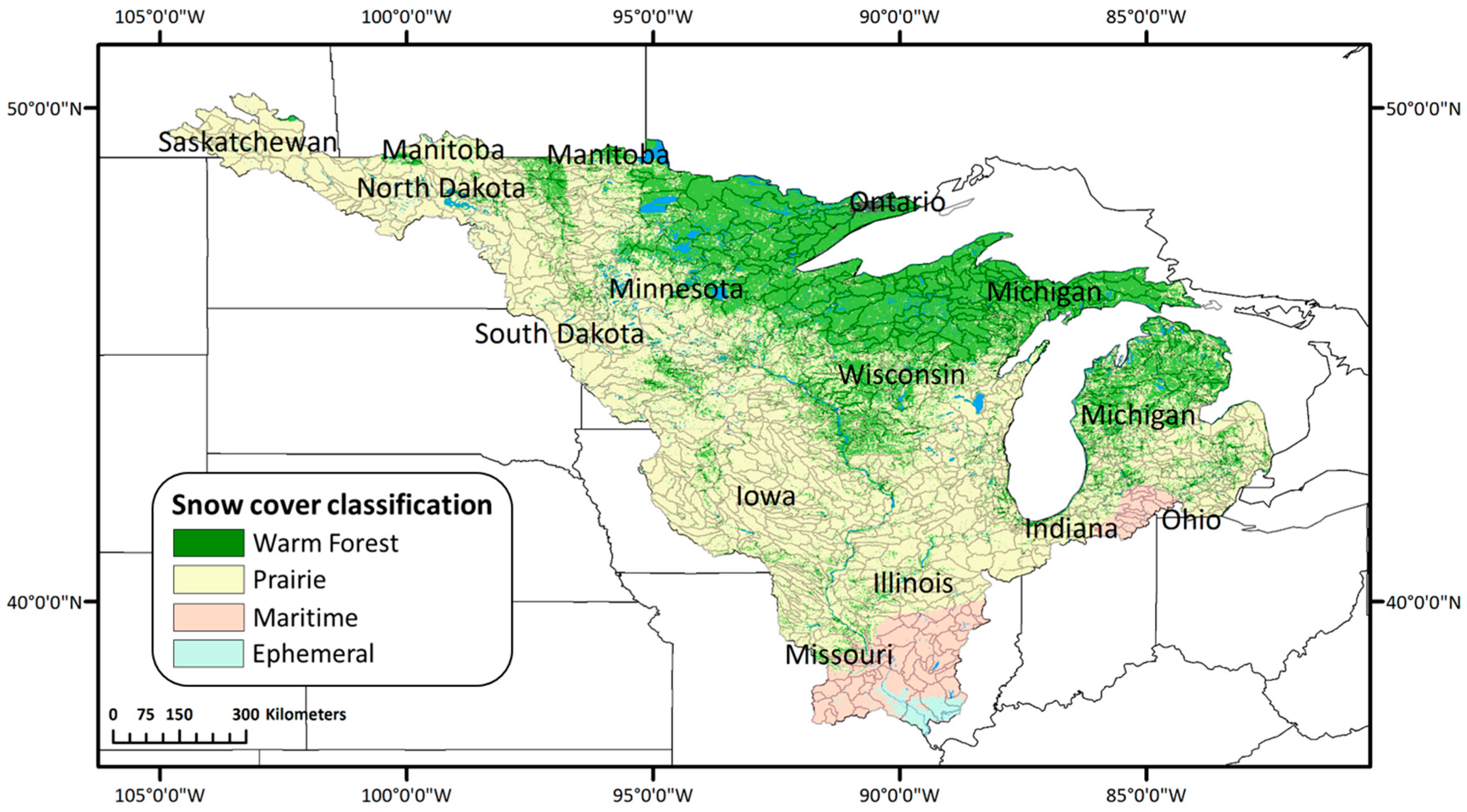
2. Study Area
3. Data and Preprocessing
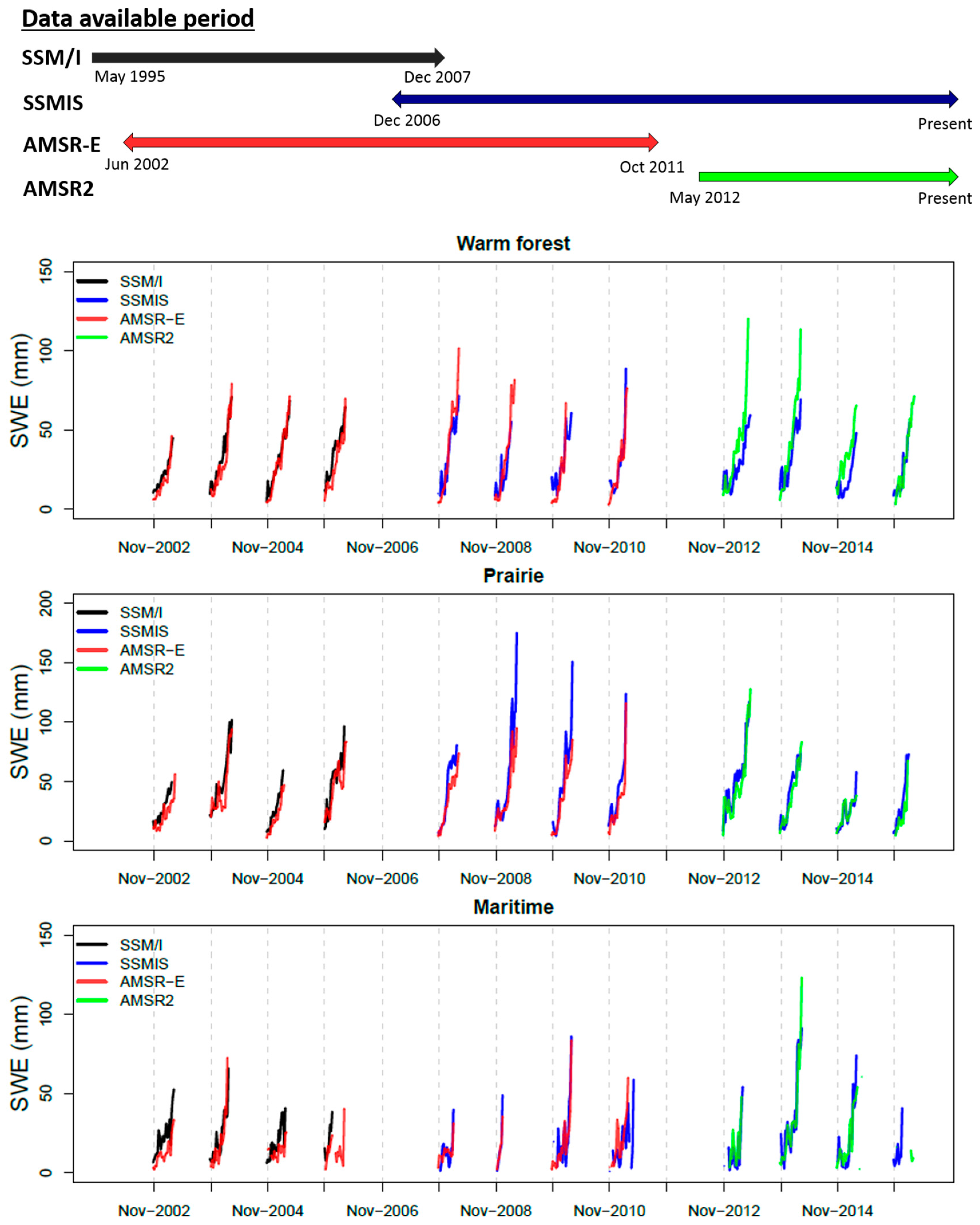
3.1. SSM/I and SSMIS SWE
3.2. AMSR2 and AMSR-E SWE
4. Methods
5. Results and Discussions
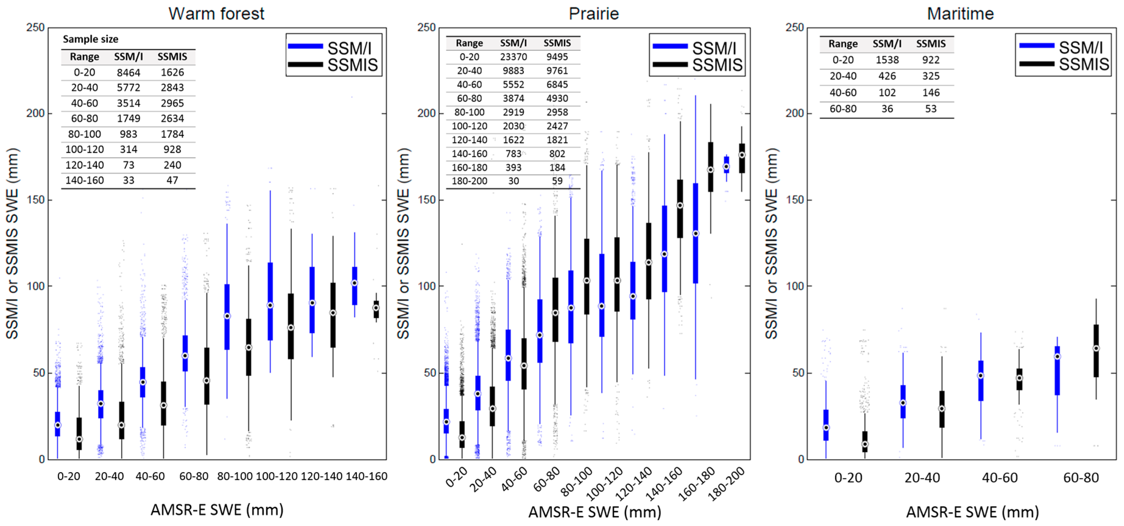
5.1. Comparison between SSM/I and SSMIS SWE
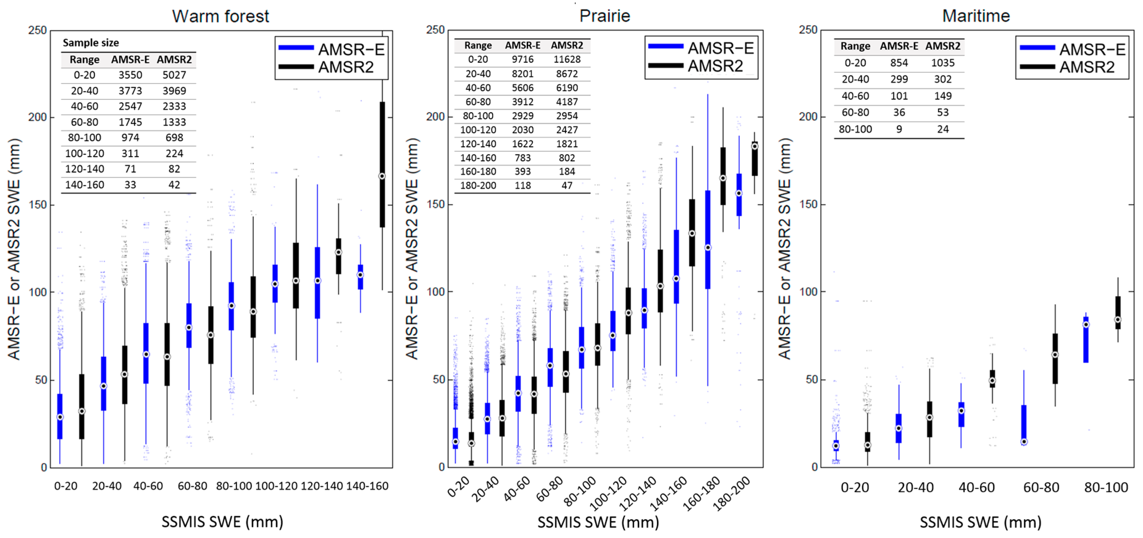
5.2. Comparison of AMSR-E and AMSR2 SWE with SSMIS SWE
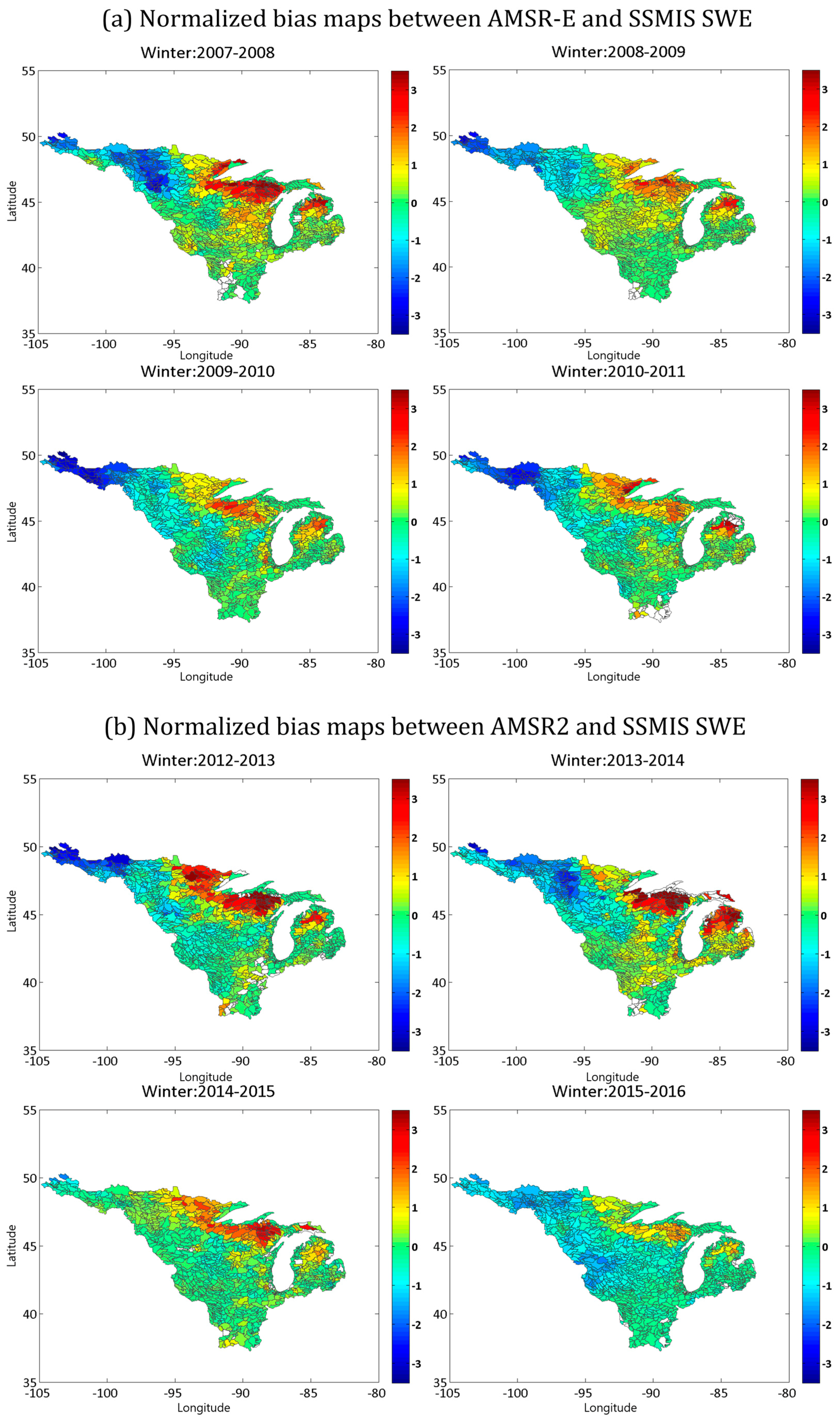
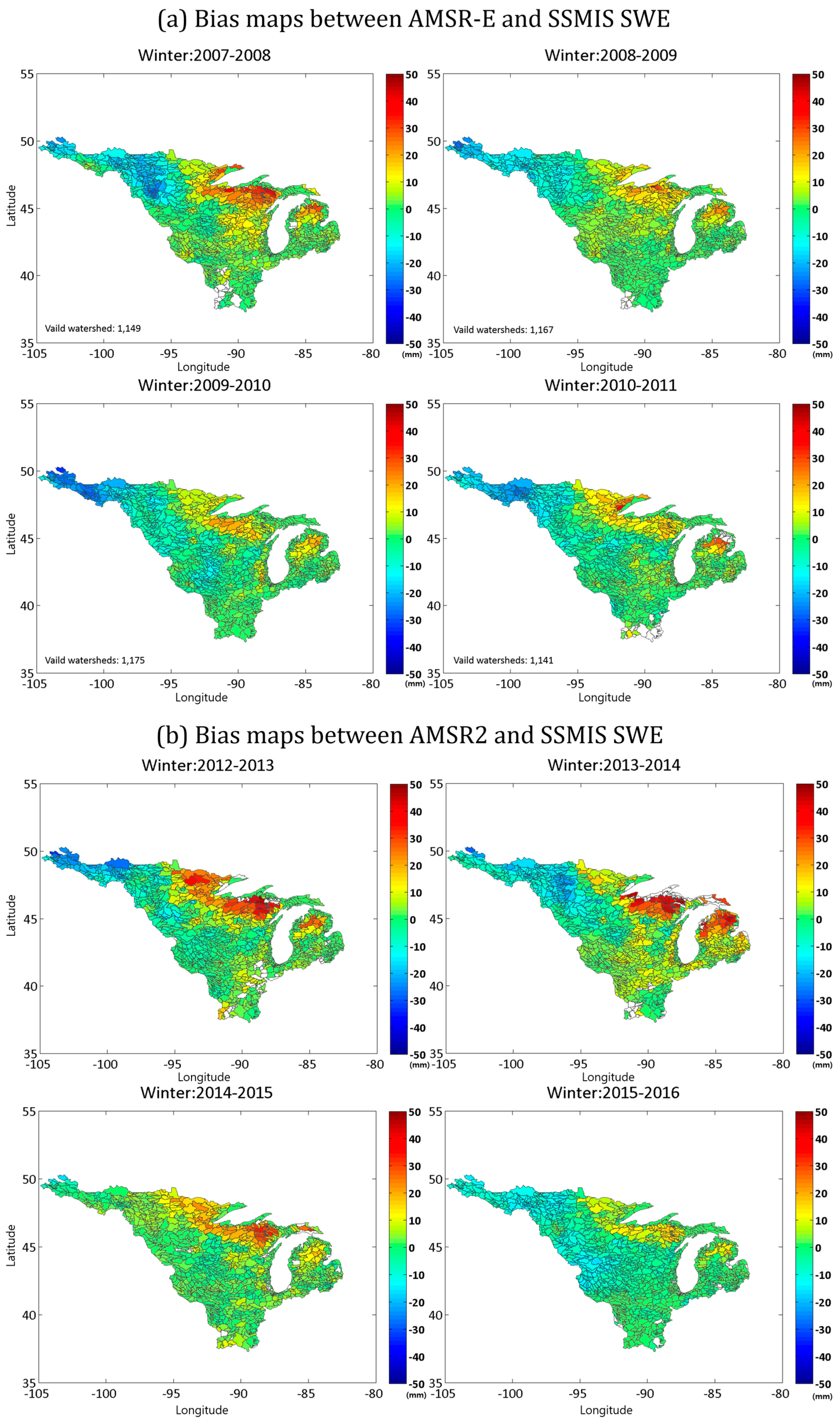
5.3. Spatial Bias Comparison between AMSR-E and AMSR2 with SSMIS SWE
6. Conclusions
Acknowledgments
Author Contributions
Conflicts of Interest
References
- Doesken, N.J.; Judson, A. The Snow Booklet: A Guide to the Science, Climatology, and Measurement of Snow in the United States; Colorado State University Publications & Printing: Fort Collins, CO, USA, 1997. [Google Scholar]
- Stocker, T. Climate Change 2013: The Physical Science Basis: Working Group I Contribution to the Fifth Assessment Report of the Intergovernmental Panel on Climate Change; Cambridge University Press: Cambridge, UK; New York, NY, USA, 2014. [Google Scholar]
- Mankin, J.S.; Viviroli, D.; Singh, D.; Hoekstra, A.Y.; Diffenbaugh, N.S. The potential for snow to supply human water demand in the present and future. Environ. Res. Lett. 2015, 10, 114016. [Google Scholar] [CrossRef]
- Berghuijs, W.R.; Woods, R.A.; Hutton, C.J.; Sivapalan, M. Dominant flood generating mechanisms across the United States. Geophys. Res. Lett. 2016, 43, 4382–4390. [Google Scholar] [CrossRef]
- Miller, J.E.; Frink, D.L. Changes in Flood Response of the Red River of the North Basin, North Dakota-Minnesota; United States Government Printing Office: Washington, DC, USA, 1984.
- Zhao, Q.; Liu, Z.; Ye, B.; Qin, Y.; Wei, Z.; Fang, S. A snowmelt runoff forecasting model coupling WRF and DHSVM. Hydrol. Earth Syst. Sci. 2009, 13, 1897–1906. [Google Scholar] [CrossRef]
- Vuyovich, C.; Jacobs, J.M. Snowpack and runoff generation using AMSR-E passive microwave observations in the Upper Helmand Watershed, Afghanistan. Remote Sens. Environ. 2011, 115, 3313–3321. [Google Scholar] [CrossRef]
- Marks, D.; Kimball, J.; Tingey, D.; Link, T. The sensitivity of snowmelt processes to climate conditions and forest cover during rain-on-snow: A case study of the 1996 Pacific Northwest flood. Hydrol. Process. 1998, 12, 1569–1587. [Google Scholar] [CrossRef]
- Armstrong, R.; Brodzik, M. An earth-gridded SSM/I data set for cryospheric studies and global change monitoring. Adv. Space Res. 1995, 16, 155–163. [Google Scholar] [CrossRef]
- Derksen, C.; Walker, A.E. Identification of systematic bias in the cross-platform (SMMR and SSM/I) EASE-grid brightness temperature time series. IEEE Trans. Geosci. Remote Sens. 2003, 41, 910–915. [Google Scholar] [CrossRef]
- Foster, J.L.; Sun, C.; Walker, J.P.; Kelly, R.; Chang, A.; Dong, J.; Powell, H. Quantifying the uncertainty in passive microwave snow water equivalent observations. Remote Sens. Environ. 2005, 94, 187–203. [Google Scholar] [CrossRef]
- Takala, M.; Luojus, K.; Pulliainen, J.; Derksen, C.; Lemmetyinen, J.; Kärnä, J.-P.; Koskinen, J.; Bojkov, B. Estimating northern hemisphere snow water equivalent for climate research through assimilation of space-borne radiometer data and ground-based measurements. Remote Sens. Environ. 2011, 115, 3517–3529. [Google Scholar] [CrossRef]
- Vuyovich, C.M.; Jacobs, J.M.; Daly, S.F. Comparison of passive microwave and modeled estimates of total watershed SWE in the continental United States. Water Resour. Res. 2014, 50, 9088–9102. [Google Scholar] [CrossRef]
- Jackson, T.J. Soil moisture estimation using special satellite microwave/imager satellite data over a grassland region. Water Resour. Res. 1997, 33, 1475–1484. [Google Scholar] [CrossRef]
- Paloscia, S.; Macelloni, G.; Santi, E.; Koike, T. A multifrequency algorithm for the retrieval of soil moisture on a large scale using microwave data from SMMR and SSM/I satellites. IEEE Trans. Geosci. Remote Sens. 2001, 39, 1655–1661. [Google Scholar] [CrossRef]
- Ramage, J.M.; Isacks, B.L. Interannual variations of snowmelt and refreeze timing on southeast-Alaskan icefields, USA. J. Glaciol. 2003, 49, 102–116. [Google Scholar] [CrossRef]
- Ramage, J.; McKenney, R.; Thorson, B.; Maltais, P.; Kopczynski, S. Relationship between passive microwave-derived snowmelt and surface-measured discharge, Wheaton River, Yukon Territory, Canada. Hydrol. Process. 2006, 20, 689–704. [Google Scholar] [CrossRef]
- Tedesco, M.; Brodzik, M.; Armstrong, R.; Savoie, M.; Ramage, J. Pan arctic terrestrial snowmelt trends (1979–2008) from spaceborne passive microwave data and correlation with the Arctic Oscillation. Geophys. Res. Lett. 2009, 36, L21402. [Google Scholar] [CrossRef]
- Takala, M.; Pulliainen, J.; Metsamaki, S.J.; Koskinen, J.T. Detection of snowmelt using spaceborne microwave radiometer data in Eurasia from 1979 to 2007. IEEE Trans. Geosci. Remote Sens. 2009, 47, 2996–3007. [Google Scholar] [CrossRef]
- Comiso, J.C.; Cavalieri, D.J.; Parkinson, C.L.; Gloersen, P. Passive microwave algorithms for sea ice concentration: A comparison of two techniques. Remote Sens. Environ. 1997, 60, 357–384. [Google Scholar] [CrossRef]
- Liu, A.; Cavalieri, D. On sea ice drift from the wavelet analysis of the Defense Meteorological Satellite Program (DMSP) Special Sensor Microwave Imager (SSM/I) data. Int. J. Remote Sens. 1998, 19, 1415–1423. [Google Scholar] [CrossRef]
- Jin, R.; Li, X.; Che, T. A decision tree algorithm for surface soil freeze/thaw classification over China using SSM/I brightness temperature. Remote Sens. Environ. 2009, 113, 2651–2660. [Google Scholar] [CrossRef]
- Kim, Y.; Kimball, J.S.; McDonald, K.C.; Glassy, J. Developing a global data record of daily landscape freeze/thaw status using satellite passive microwave remote sensing. IEEE Trans. Geosci. Remote Sens. 2011, 49, 949–960. [Google Scholar] [CrossRef]
- Kelly, R.E.; Chang, A.T.; Tsang, L.; Foster, J.L. A prototype AMSR-E global snow area and snow depth algorithm. IEEE Trans. Geosci. Remote Sens. 2003, 41, 230–242. [Google Scholar] [CrossRef]
- Kelly, R. The AMSR-E snow depth algorithm: Description and initial results. J. Remote Sens. Soc. Jpn. 2009, 29, 307–317. [Google Scholar]
- Tedesco, M.; Narvekar, P.S. Assessment of the NASA AMSR-E SWE Product. IEEE J. Sel. Top. Appl. Earth Observ. Remote Sens. 2010, 3, 141–159. [Google Scholar] [CrossRef]
- Kelly, R.E. Status of AMSR2 Level-2 Products (Algorithm Ver. 1.00)—Snow Depth; JAXA Earth Observation Research Center: Saitama, Japan, 2013. [Google Scholar]
- Kelly, R.E. Status of AMSR2 Level-2 Products (Algorithm Ver. 2.00)—8. Snow Depth; JAXA Earth Observation Research Center: Saitama, Japan, 2015. [Google Scholar]
- Armstrong, R.L.; Brodzik, M.J. Recent northern hemisphere snow extent: A comparison of data derived from visible and microwave satellite sensors. Geophys. Res. Lett. 2001, 28, 3673–3676. [Google Scholar] [CrossRef]
- Derksen, C.; Walker, A.; LeDrew, E.; Goodison, B. Combining SMMR and SSM/I data for time series analysis of central North American snow water equivalent. J. Hydrometeorol. 2003, 4, 304–316. [Google Scholar] [CrossRef]
- Cavalieri, D.J.; Parkinson, C.L.; DiGirolamo, N.; Ivanoff, A. Intersensor Calibration Between F13 SSMI and F17 SSMIS for Global Sea Ice Data Records. IEEE Geosci. Remote Sens. Lett. 2012, 9, 233–236. [Google Scholar] [CrossRef]
- Okuyama, A.; Imaoka, K. Intercalibration of Advanced Microwave Scanning Radiometer-2 (AMSR2) Brightness Temperature. IEEE Trans. Geosci. Remote Sens. 2015, 53, 4568–4577. [Google Scholar] [CrossRef]
- Meier, W.N.; Khalsa, S.J.S.; Savoie, M.H. Intersensor calibration between F-13 SSM/I and F-17 SSMIS near-real-time sea ice estimates. IEEE Trans. Geosci. Remote Sens. 2011, 49, 3343–3349. [Google Scholar] [CrossRef]
- Stadnyk, T.; Dow, K.; Wazney, L.; Blais, E.-L. The 2011 flood event in the Red River Basin: Causes, assessment and damages. Can. Water Resour. J. 2016, 41, 65–73. [Google Scholar] [CrossRef]
- Wazney, L.; Clark, S.P. The 2009 flood event in the Red River Basin: Causes, assessment and damages. Can. Water Resour. J. 2016, 41, 56–64. [Google Scholar] [CrossRef]
- Tuttle, S.E.; Cho, E.; Restrepo, P.J.; Jia, X.; Vuyovich, C.M.; Cosh, M.H.; Jacobs, J.M. Remote Sensing of Drivers of Spring Snowmelt Flooding in the North Central U.S. In Remote Sensing of Hydrological Extremes; Lakshmi, V., Ed.; Springer International Publishing: Cham, Switzerland, 2017; pp. 21–45. [Google Scholar]
- Hirsch, R.; Ryberg, K. Has the magnitude of floods across the USA changed with global CO2 levels? Hydrol. Sci. J. 2012, 57, 1–9. [Google Scholar] [CrossRef]
- Melesse, A.M. Spatiotemporal dynamics of land surface parameters in the Red River of the North Basin. Phys. Chem. Earth Parts A/B/C 2004, 29, 795–810. [Google Scholar] [CrossRef]
- Sturm, M.; Taras, B.; Liston, G.E.; Derksen, C.; Jonas, T.; Lea, J. Estimating Snow Water Equivalent Using Snow Depth Data and Climate Classes. J. Hydrometeorol. 2010, 11, 1380–1394. [Google Scholar] [CrossRef]
- Liston, G.; Sturm, M. A global snow-classification dataset for earth-system applications. Unpublished work. 2014. [Google Scholar]
- Sturm, M.; Holmgren, J.; Liston, G.E. A seasonal snow cover classification system for local to global applications. J. Clim. 1995, 8, 1261–1283. [Google Scholar] [CrossRef]
- Kunkee, D.B.; Poe, G.A.; Boucher, D.J.; Swadley, S.D.; Hong, Y.; Wessel, J.E.; Uliana, E.A. Design and Evaluation of the First Special Sensor Microwave Imager/Sounder. IEEE Trans. Geosci. Remote Sens. 2008, 46, 863–883. [Google Scholar] [CrossRef]
- Armstrong, R.; Knowles, K.; Brodzik, M.; Hardman, M. DMSP SSM/I-SSMIS Pathfinder Daily EASE-Grid Brightness Temperatures, Version 2; NASA National Snow Ice Data Center Distributed Active Archive Center: Boulder, CO, USA, 1994; Updated 2016; Available online: http://nsidc.org/data/docs/daac/nsidc0032_ssmi_ease_tbs.gd.html (accessed on 5 May 2016).
- Chang, A.; Foster, J.; Hall, D.K. Nimbus-7 SMMR derived global snow cover parameters. Ann. Glaciol. 1987, 9, 39–44. [Google Scholar] [CrossRef]
- Chang, A.; Foster, J.; Hall, D.; Goodison, B.E.; Walker, A.E.; Metcalfe, J.; Harby, A. Snow parameters derived from microwave measurements during the BOREAS winter field campaign. J. Geophys. Res. Atmos. 1997, 102, 29663–29671. [Google Scholar] [CrossRef]
- Derksen, C.; LeDrew, E.; Walker, A.; Goodison, B. Influence of sensor overpass time on passive microwave-derived snow cover parameters. Remote Sens. Environ. 2000, 71, 297–308. [Google Scholar] [CrossRef]
- Imaoka, K.; Kachi, M.; Kasahara, M.; Ito, N.; Nakagawa, K.; Oki, T. Instrument performance and calibration of AMSR-E and AMSR2. Int. Arch. Photogramm. Remote Sens. 2010, 38, 13–18. [Google Scholar]
- Tedesco, M.; Kelly, R.; Foster, J.; Chang, A. AMSR-E/Aqua Daily L3 Global Snow Water Equivalent EASE-Grids V002; NASA National Snow Ice Data Center Distributed Active Archive Center: Boulder, CO, USA, 2004. [Google Scholar]
- Kelly, R.E.; University of Waterloo, Waterloo, ON, Canada. Personal communication, 2016.
- Brodzik, M.J. F17 vs. F13 SWE Regression. Available online: http://cires1.colorado.edu/~brodzik/F13-F17swe/ (accessed on 20 January 2017).
- Dong, J.; Walker, J.P.; Houser, P.R. Factors affecting remotely sensed snow water equivalent uncertainty. Remote Sens. Environ. 2005, 97, 68–82. [Google Scholar] [CrossRef]
- Kelly, R.E.J.; Chang, A.T.C. Development of a passive microwave global snow depth retrieval algorithm for Special Sensor Microwave Imager (SSM/I) and Advanced Microwave Scanning Radiometer-EOS (AMSR-E) data. Radio Sci. 2003, 38. [Google Scholar] [CrossRef]
- Lee, Y.-K.; Kongoli, C.; Key, J. An In-Depth Evaluation of Heritage Algorithms for Snow Cover and Snow Depth Using AMSR-E and AMSR2 Measurements. J. Atmos. Ocean. Technol. 2015, 32, 2319–2336. [Google Scholar] [CrossRef]
- Langlois, A.; Royer, A.; Dupont, F.; Roy, A.; Goita, K.; Picard, G. Improved Corrections of Forest Effects on Passive Microwave Satellite Remote Sensing of Snow Over Boreal and Subarctic Regions. IEEE Trans. Geosci. Remote Sens. 2011, 49, 3824–3837. [Google Scholar] [CrossRef]
- Roy, A.; Royer, A.; Hall, R.J. Relationship between forest microwave transmissivity and structural parameters for the Canadian boreal forest. IEEE Geosci. Remote Sens. Lett. 2014, 11, 1802–1806. [Google Scholar] [CrossRef]


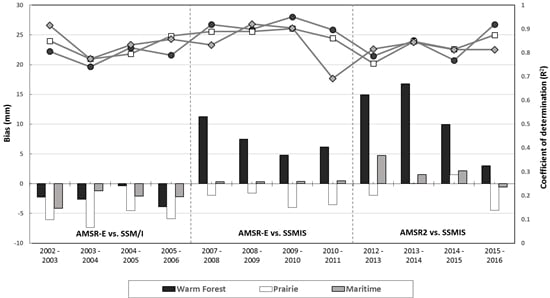
| Bias (mm) | R2 | ||||||
|---|---|---|---|---|---|---|---|
| Snow Class | Warm Forest | Prairie | Maritime | Warm Forest | Prairie | Maritime | |
| AMSR-E & SSM/I | 2003 | −2.23 | −6.06 | −4.12 | 0.81 | 0.85 | 0.91 |
| 2004 | −2.61 | −7.35 | −1.22 | 0.74 | 0.77 | 0.77 | |
| 2005 | −0.37 | −4.51 | −2.11 | 0.82 | 0.80 | 0.83 | |
| 2006 | −3.85 | −5.88 | −2.17 | 0.79 | 0.87 | 0.86 | |
| Aver. | −2.26 | −5.95 | −2.41 | 0.79 | 0.82 | 0.84 | |
| AMSR-E & SSMIS | 2008 | 11.24 | −1.94 | 0.31 | 0.92 | 0.89 | 0.83 |
| 2009 | 7.48 | −1.60 | 0.31 | 0.90 | 0.89 | 0.92 | |
| 2010 | 4.82 | −3.99 | 0.36 | 0.95 | 0.90 | 0.90 | |
| 2011 | 6.14 | −3.51 | 0.47 | 0.90 | 0.86 | 0.69 | |
| Aver. | 7.42 | −2.76 | 0.36 | 0.92 | 0.88 | 0.84 | |
| AMSR2 & SSMIS | 2013 | 14.94 | −1.94 | 4.73 | 0.79 | 0.76 | 0.82 |
| 2014 | 16.78 | 0.00 | 1.55 | 0.85 | 0.85 | 0.84 | |
| 2015 | 9.93 | 1.50 | 2.15 | 0.77 | 0.81 | 0.81 | |
| 2016 | 3.02 | −4.46 | −0.59 | 0.92 | 0.87 | 0.81 | |
| Aver. | 11.16 | −1.22 | 1.96 | 0.83 | 0.82 | 0.82 | |
© 2017 by the authors. Licensee MDPI, Basel, Switzerland. This article is an open access article distributed under the terms and conditions of the Creative Commons Attribution (CC BY) license (http://creativecommons.org/licenses/by/4.0/).
Share and Cite
Cho, E.; Tuttle, S.E.; Jacobs, J.M. Evaluating Consistency of Snow Water Equivalent Retrievals from Passive Microwave Sensors over the North Central U. S.: SSM/I vs. SSMIS and AMSR-E vs. AMSR2. Remote Sens. 2017, 9, 465. https://doi.org/10.3390/rs9050465
Cho E, Tuttle SE, Jacobs JM. Evaluating Consistency of Snow Water Equivalent Retrievals from Passive Microwave Sensors over the North Central U. S.: SSM/I vs. SSMIS and AMSR-E vs. AMSR2. Remote Sensing. 2017; 9(5):465. https://doi.org/10.3390/rs9050465
Chicago/Turabian StyleCho, Eunsang, Samuel E. Tuttle, and Jennifer M. Jacobs. 2017. "Evaluating Consistency of Snow Water Equivalent Retrievals from Passive Microwave Sensors over the North Central U. S.: SSM/I vs. SSMIS and AMSR-E vs. AMSR2" Remote Sensing 9, no. 5: 465. https://doi.org/10.3390/rs9050465