
Glacier Changes in the Susitna Basin, Alaska, USA, (1951–2015) using GIS and Remote Sensing Methods


1
Institut für Geographie, Friedrich-Alexander-Universität Erlangen-Nürnberg, Erlangen 91058, Germany
2
Geophysical Institute, University of Alaska Fairbanks, Fairbanks 99775, AK, USA
3
Department of Earth Sciences, Uppsala University, Uppsala 74010, Sweden
*
Author to whom correspondence should be addressed.
Remote Sens. 2017, 9(5), 478; https://doi.org/10.3390/rs9050478
Submission received: 18 March 2017
/
Revised: 1 May 2017
/
Accepted: 5 May 2017
/
Published: 14 May 2017
(This article belongs to the Special Issue Remote Sensing of Glaciers)
Abstract
:The Susitna River draining from the highly glacierized Central Alaska Range has repeatedly been considered a potential hydro-power source in recent decades, raising questions about the effect of glacier changes on the basin’s river runoff. We determine changes in the glacier area (1951–2010), elevation (1951–2010, 1951–2005 and 2005–2010), equilibrium line altitude (ELA, 1999–2015), and accumulation area ratio (AAR, 1999–2015) of the basin’s five largest glaciers covering 587 km² (2010). We use the Landsat time series, as well as digital elevation models (DEMs) from 1951 (United States Geological Survey (USGS) aerial imagery), 2005 (Advanced Spaceborne Thermal Emission and Reflection Radiometer, ASTER), and 2010 (airborne interferometric synthetic aperture radar, IfSAR). The glaciers lost an area of 128 ± 15 km² (16%) between 1951 and 2010. The mean ELA was located at 1745 ± 88 m a.s.l. during 1999–2015. The glacier’s annual ELAs do not show any significant trends. We found a glacier-wide elevation change of −0.41 ± 0.07 m yr−1 for the period 1951–2005 and −1.20 ± 0.25 m yr−1 for 2005–2010. The results indicate that the glaciers are in a state of retreat and thinning, and have been losing mass at an accelerated rate in recent years. The interpretation of the thickness changes is complicated by the glaciers’ surge cycles.
1. Introduction
Alaskan glaciers have been important contributors to the sea level rise in recent decades, with estimated mass losses of 52 ± 15 Gt yr−1 for the period of the mid-1950s to the mid-1990s [1], 41.9 ± 8.6 Gt yr−1 for the period 1962–2006 [2], and 75 ± 11 Gt yr−1 for 1994 to 2013 [3]. For the more recent period of 2003–2009, Gardner, et al. [4] estimate a mass loss of 52 ± 17 Gt yr−1, corresponding to an average thinning of 0.57 ± 0.20 m w.e. yr−1. Various studies show accelerated mass losses in many regions in recent years [1,5,6]. The glacier changes are consistent with a near-surface temperature increase in Alaska of + 1.9 C between 1949 and 2005 [7]. Coincident with the mass changes, Alaskan glaciers have retreated and shrunk in area. Loso, et al. [8] investigated the change in glacier area for glaciers in the Alaskan National Parks between 1948 and 2011. They found an area loss of 8% for all investigated glaciers, with considerable variations between the individual park units.
This study focuses on the glaciers in the Susitna River basin in the Central Alaska Range (Figure 1), and aims to merge data from various satellite and airborne products in order to examine glacier changes during the period 1951–2015. The study area was initially chosen because the Susitna River has been subject to plans for hydro-power extraction for several decades [9,10,11]; however, these projects are no longer being pursued. We determine the glacier area changes between 1951 and 2010, glacier elevation changes, and mass losses for the periods 1951–2005, 2005–2010, and 1951–2010. Additionally, we derive annual late summer snow line altitudes as an approximation for the equilibrium line altitudes (ELAs) and determine the accumulation area ratios (AARs) for the period 1999–2015. These variables provide valuable proxies to assess the response of glaciers to climate change [12,13,14].
2. Study Site
Glaciers are found in the upper reaches of the Susitna drainage basin and cover only 5% (670 km²) of the total basin area (referring to the proposed Watana dam site [9]). Nevertheless, their contribution to the river runoff is significant. Clarke, et al. [10] found that between 1981 and 1983, the glaciers contributed about 13% of the river’s seasonal runoff at the Gold Creek gauging station, which is located several hundred kilometers further downstream of the glaciers. The annual basin precipitation ranges from 1500 to 2000 mm [15], with a seasonal maximum in summer [7].
The basin includes five large glaciers: The West Fork, Susitna, East Fork, MacLaren, and Eureka Glaciers (Figure 1). The glaciers’ termini elevations ranged from approximately 820 m a.s.l. (Susitna) to 1130 m a.s.l. (Eureka) in 2010. The highest glacier reaches are located at an elevation of 4000 m a.s.l. Roughly 24% of the five large glaciers’ total area was debris-covered in 2010 (Figure 1), with the highest percentages found on the Susitna Glacier (29%) and West Fork Glacier (19%).
The abundance of surge-type glaciers in the basin is well documented (e.g., [16]). A surge-type glacier’s inherent surge cycle typically includes a thickening (quiescent phase) lasting several decades, followed by a thinning (surge phase) of the glacier’s reservoir zone in the order of tens of meters over a period ranging from months to a few years [17]. A surge leads to significant displacements of ice masses and often glacier advance [17], and hence complicates the climate interpretation of the glacier area and elevation changes in the study area. Susitna Glacier last surged in 1951/52. A recurrence interval of 50–60 years has been estimated [16,18,19], but no signs of an imminent surge have been observed since. West Fork Glacier surged in 1935 and again in 1987/88 [18]. The East Fork, MacLaren, and Eureka Glaciers have been described to be of weak surge character, with only little vertical change seen during a surge [16,18,19].
3. Data and Methods
3.1. Area Changes
To analyze the glacier area changes between 1951 and 2010, we derived the initial glacier outlines from topographic maps (1:63,360 scale) produced by the USGS from aerial photographs (Table 1). The maps refer to different dates between 1948 and 1954 with the exact dates unknown, so we assume the data reflects the conditions of 1951.
The topographic maps were available as digital raster graphics. We used a Geographic Information System (GIS) to manually extract the glacier outlines from the digital raster graphics to convert them into vectorized polygons. The ~2010 outlines were taken from the Randolph glacier inventory derived from optical imagery (mostly Landsat) [20,21].
In the case that a glacier split into several smaller glaciers during the period investigated, the smaller glaciers were allocated to the glacier they belonged to in the earlier period.
3.2. Elevation and Mass Changes
Elevation changes were computed from DEM differencing using elevation data from 1951, 2005, and 2010. The 1951 DEM was compiled by the USGS using standard stereo-photogrammetric techniques [22]. The 2005 ASTER DEM is based on two scenes taken at the end of the ablation season, encompassing most of the Susitna basin with only little cloud cover. However, due to the limited satellite swath, large parts of the Eureka Glacier are missing in the ASTER DEM. The ASTER DEM was generated by the NASA Land Processes Distributed Active Archive Center (LP DAAC). The IfSAR data was derived from airborne X-band radar data flown over the study area in summer 2010 [23].
Prior to deriving elevation changes, all DEMs were reprojected to the NAD83 Alaska Albers coordinate system. The ASTER and IfSAR DEM were regridded to a 40 m pixel resolution prior to differencing with the NED DEM. The DEMs were co-registered in the x, y, and z direction across 800 km² of ice-free terrain (terrain that is free of ice and water for all three dates), following the approach by [24]. Before differencing with the ASTER DEM, the NED DEM was shifted 123 m in the x, 17 m in the y, and −13 m in the z direction. Before differencing with the IfSAR DEM, the NED DEM was shifted 115 m in the x, 27 m in the y, and −13 m in the z direction. These large shifts are not unexpected given the poor ground control available during the derivation of the 1950 DEM [1]. Note that the vertical shift also accounts for the different vertical datums of the two datasets, which were not explicitly corrected before the coregistration.
Prior to the ASTER/IfSAR DEM differencing, the former was shifted 5 m in the x, 14 m in the y, and 0.6 m in the z direction. We also checked for elevation dependent biases by regressing elevation against dh (third degree polynomial regression), but did not detect obvious elevation dependent biases. We included this step, as the ASTER DEM might be affected by a distortion of the z-scale, caused by poorly resolved stereo orientation [24]. Figure 2 shows the frequency distribution of elevation changes dh over stable terrain before and after the applied corrections. Despite the correction, the distributions of the dh values deviate from a normal distribution, suggesting some remaining non-random elevation differences between the DEMs. This is not unexpected, because our approach cannot account for higher order shifts between DEMs.
In a last step, the co-registered DEMs were subtracted from each other to calculate dh over the glacierized areas. To eliminate outliers, dh/dt values higher than 5 m yr−1 and smaller than −15 m yr−1 were considered unrealistic and interpolated based on surrounding pixel values. In total, roughly 1.5% of the total glacier area was treated in this way for the period 2005–2010. No such correction was necessary for the periods 1951–2005 and 1951–2010. Values were also interpolated in all areas of the 2005 ASTER DEM that were affected by cloud cover.
Glacier volume changes were computed for the three periods: 1951–2005 (ASTER-NED DEM), 2005–2010 (IfSAR-ASTER DEM), and 1951–2010 (IfSAR-NED DEM). The dh values were transformed into per-pixel volume changes by multiplying dh by the raster area. The total volume changes were then converted into mass changes. We assumed a spatially constant density of 850 kg m−³. This is lower than the density of ice to account for the removal of lower-density firn layers. No spatially distributed firn correction was applied; the factor of 850 kg m−³ has been found to be appropriate for a wide range of conditions [25].
To analyze the elevation dependencies, dh values were averaged over elevation bands of 50 m using the area-altitude distribution of the NED DEM and the 1951 glacier outlines for the periods 1951–2005 and 1951–2010, the IfSAR DEM, and the 2010 glacier outlines for the period 2005–2010. To compute specific mass changes, we divided the mass change by the arithmetic mean of the earlier and later year’s glacier area. In the absence of data, we assume that the glacier areas for 2005 are identical to the 2010 area.
3.3. Equilibrium Line Altitudes and Accumulation Area Ratios
We manually digitized the end of summer snowline altitudes for 14 years between 1999 and 2015 based on a visual inspection of Landsat images (Appendix A). The years before 1999 were not included because, during the ten years prior to this, only one year (1995) presented sufficient cloud-free images to determine the annual snowlines. The snowline on the glacier can usually be detected as the margin of the previous year’s clean white snow cover [13,26,27]. We use data from the Landsat 5, 7, and 8 sensors TM, ETM+, and OLI, respectively, which have proved useful for this task in previous studies [14,28,29]. Following [28], the combination of spectral bands 5, 4, 3 for Landsat 8OLI and 4, 3, 2 for Landsat TM/ETM+ were used to discriminate snow cover from ice. Images were available every one to two weeks, as the repetition cycle at the high latitudes analyzed here is higher than at mid-latitudes due to the larger overlap of neighboring paths. We aimed at producing images depicting the end of summer state, when the snow cover is at a minimum and the transient snowline approaches the maximum altitude for the current year. All imagery that was acquired between the beginning of August and mid-September was evaluated. In 2003, two images were used: one refers to the end of July, the other to mid-August (Table 5). The end of July image was used to check the mid-August image, as the latter was missing a part of the Eureka glacier. The middle of September usually marks the end of the ablation season in central Alaska [2]. For each year, we used the latest available image during this period that was sufficiently cloud-free to allow the snowlines to be determined. In our time series, four years are missing (2000, 2007, 2011, and 2014) due to the lack of cloud-free images.
Field observations [9] indicate that superimposed ice, which originates from refreezing melt water on the glacier surface, is negligible. Thus, the derived snowlines are equivalent to equilibrium lines. For each year, the ELA was computed as the mean of the elevations of all DEM pixels along the snowline for each of the five large glaciers. We extracted the elevations from the IFSAR DEM, since this DEM is the most precise and reflects the glaciers’ elevation close to the Landsat image acquisitions [14]. Trends for the ELA were calculated by performing a linear regression analysis on the annual time series. The area above the ELA was determined to calculate the accumulation area ratio (AAR), i.e., the ratio of the accumulation area to the total glacier area.
4. Uncertainty Estimation
4.1. Area Changes
Previous studies estimate an uncertainty of 10% for Alaskan glacier outlines based on the USGS topographic maps [2]. Kienholz, et al. [20] report an error of 6% for the modern glacier outlines. Assuming the uncertainties are independent, they were combined in quadrature. This results in an error of 12% for the area change calculations.
4.2. DEM-Differencing
The absolute vertical accuracy of the NED DEM at the pixel scale is estimated to be 15 m in the ablation area and 45 m in the accumulation area [1]. For the IfSAR DEM, a vertical accuracy of 3 m is reported [30]. For the ASTER DEM, Berthier,et al. [2] reports vertical errors in the range of 15 m. Poor ground control and a lack of contrast between areas of ice and surrounding areas of snow cover lead to errors in the NED DEM [22]. Errors in the ASTER DEM are related to a poor orientation of the stereo-scenes, which either stems from imperfect matching procedures or imperfect image quality due to a lack of contrast, cloud cover, shadows, or topographic distortions. These errors are mostly of a random nature, rather than a systematic one [31]. Errors in the IfSAR DEM are mostly anticipated in steep areas, were radar systems perform poorly [32,33]. The IfSAR DEM quality is further influenced by the radar signal return strength that depends on surface properties such as roughness, moisture content, and snow density [34]. The data were acquired flying from three different directions to avoid shadow and layover problems. Only very few areas should be affected by these problems, mostly in the very steep areas that are not glacierized.
To quantify the uncertainties, the DEMs were differenced over non-glacierized terrain and the standard deviation σ of all dh values was assumed to represent the pixel scale uncertainty. Errors may cancel out, especially when elevation changes are investigated over large regions. In order to account for the error reduction due to the spatial averaging of σ, the standard error Se was introduced. Se was calculated by dividing σ by the number of independent observations Nind not affected by spatial autocorrelation [2,35,36]. Nind was calculated by:
where Ntot is the total pixel number, Pres the pixel size [m], and d [m] is the decorrelation length [35,37,38]. We performed a semi-variogram analysis to find d based on the dh values over stable terrain. Values for d were 2650 m for the differencing of the ASTER-IfSAR DEM, 1780 m for NED-IfSAR, and 4000 m for NED-ASTER DEMs, respectively. All values are rather high compared to other studies [2]. This points to the fact that the co-registration approach did not eliminate all mismatches between the DEMs. Indeed, visual inspection suggests that autocorrelated dh values remain across certain subregions, likely due to local shifts in the 1950 DEM.
We calculated Se for the five large glaciers individually and the remaining small glaciers combined. To account for the error in mass changes, Se was converted to mass in the same way as the dh values (see chapter 3.2).
4.3. Equilibrium Line Altitudes
The horizontal error that arises when delineating the equilibrium line is estimated to be within one Landsat pixel (i.e., 30 m). The possible horizontal dislocation of the ELA would cause an error in the vertical direction, which can be quantified by multiplying the pixel size by the slope of the glacier in the vicinity of the ELA [28]. A second source of errors is the vertical accuracy of the DEM. Rabatel, et al. [14] proposed to add the standard deviation of the elevation of the pixels along the equilibrium line to obtain the total uncertainty budget. For every glacier, the uncertainty EELA was calculated individually by:
where EDEM is the uncertainty in the elevation of the DEM, which is 3 m in this case (IfSAR DEM, Section 4.2); σELA is the standard deviation [m a.s.l.]; α is the mean slope within 30 m of the ELA based on the IfSAR DEM; and Apixel is the pixel area. Uncertainties tend to be higher on the West Fork, Susitna, and East Fork Glaciers, as these glaciers have rather high ELAs in steep terrain. Our error estimates do not include the systematic error arising from ELAs being determined before the end of the melt season.
5. Results
5.1. Area Changes
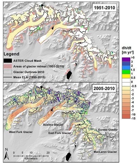
The glaciers’ area loss between 1951 and 2010 accumulates to 128 ± 15 km², which is roughly 16% of the initial area. The combined smaller glaciers (termed as “Others” in Table 2 and Table 3) account for the highest loss, both in the absolute area and expressed as a percentage (42%). Of the five largest glaciers, West Fork Glacier lost the greatest absolute area (35.0 ± 4.2 km²). The glacier terminus positions of the large glaciers in the basin receded to higher altitudes. West Fork’s and Eureka’s retreat was approximately 2 km. East Fork’s and MacLaren’s snouts retreated 1.5 km, while Susitna’s terminus remained mostly stable. The glaciers also experienced a reduction in width, which indicates a lowering of the surface [39].
5.2. Spatial Patterns in Elevation Change
The spatial distribution of surface elevation changes and the elevation changes as a function of elevation are shown in Figure 3 and Figure 4, respectively. The overall spatial pattern of the elevation changes is similar for both periods, with little change or thickening in the uppermost reaches and increasing thinning rates towards the glacier front. In contrast to the other glaciers, Susitna Glacier shows little to no change during the period 1951 to 2010 over a large portion of the glacier tongue (roughly the lowest ~6 km at ~850–900 m a.s.l.) (Figure 3). Note that a zero change is not visible around this elevation in Figure 4c, d. The surface slope is low over large areas of the glacier tongue and therefore, the corresponding 50 m elevation bins include areas with substantial thinning.
Over the longer study period of 1951–2010, we find the highest thinning rates on West Fork Glacier, where tributary A (Figure 1) used to flow into the main trunk. During the 1987/88 surge, a lake emerged, into which the tributary began calving [40]. This might explain the pronounced shrinkage of the ice in this region, as calving processes, together with lacustrine melting, can cause an accelerating mass loss [41,42].
During the same period, the tributary (B, Figure 1) to the south of West Fork Glacier’s main trunk depicts an increase in the glacier surface elevation. We attribute these positive dh changes to erroneous elevation values in the NED DEM. The pattern is missing in the period 2005–2010, supporting this interpretation. Areas of positive dh/dt values are also found in the period 2005–2010, particularly in the upper reaches of the glaciers. Since thickening and thinning areas alternate at spatially small scales, we assume that the thickening is at least partly due to errors in the ASTER DEM.
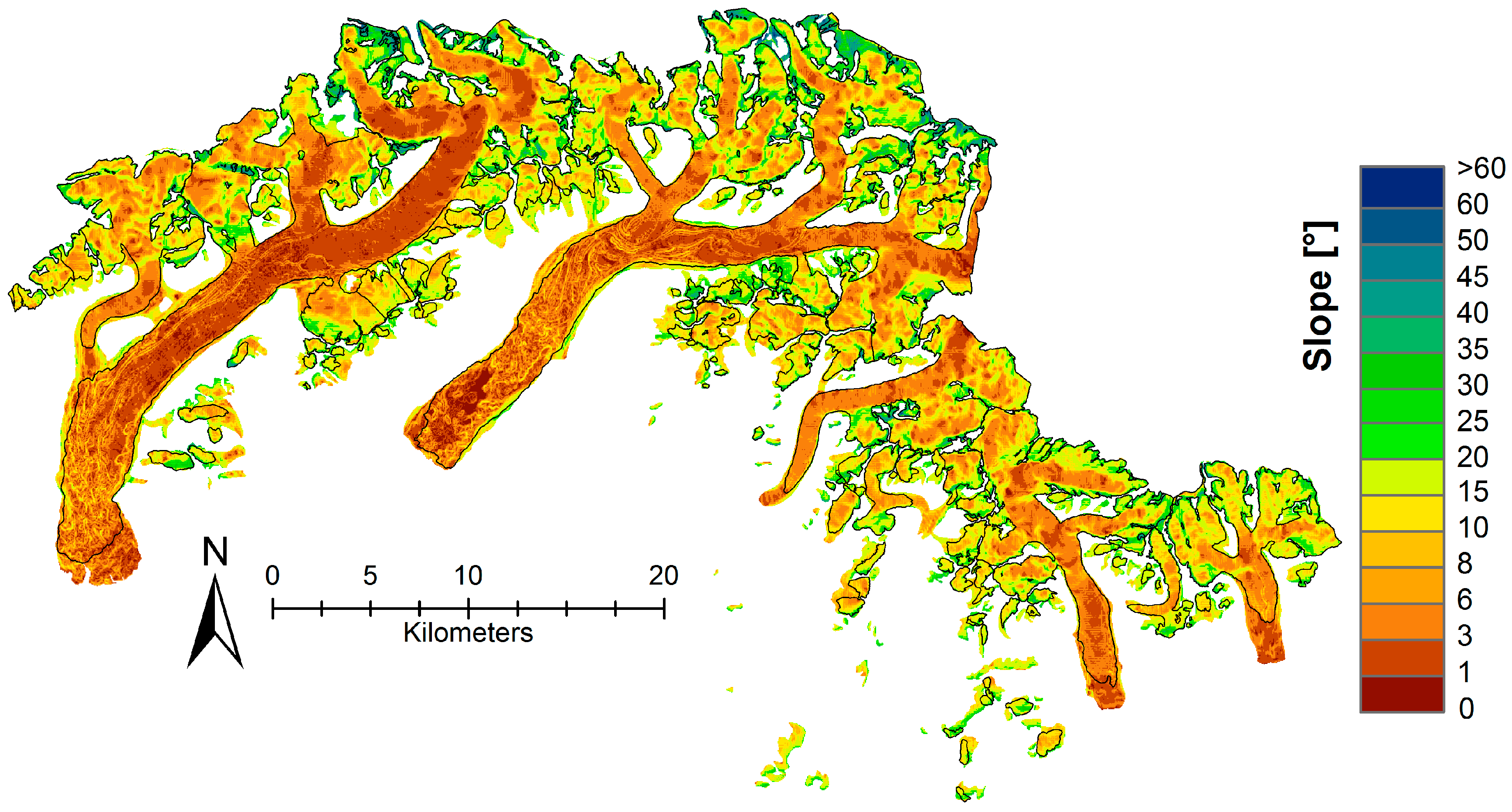
Figure 4c, d indicates that beyond 2700 m a.s.l., Susitna Glacier shows a steady thickening, while no elevation change is seen on West Fork Glacier, except for the very highest elevations. These upper reaches of the glaciers only include a very small fraction of the glacier area and are located in relatively steep terrain (Figure 5). Hence, uncertainties in the average elevation-dependent thickness change can be expected to be larger than over the lower parts of the glaciers.
Similar observations by [23], indicating errors in the NED DEM in the accumulation area of the adjacent Black Rapids Glacier, support this interpretation. Errors in the DEM may also affect other regions; however, they are difficult to detect without additional information. Thickening appears close to West Fork’s terminus. It is unclear if the thickening is due to errors in the DEMs or is caused by small-scale morphological processes typical of heavily debris-covered ice. Thickening is also found on the lower tongue of McLaren Glacier (around 1100 m–1300 m a.s.l., Figure 4) between 2005 and 2010, which is most likely attributed to errors in the ASTER DEM.
5.3. Glacier-wide Elevation and Mass Changes
Derived glacier-wide elevation and mass changes are summarized in Table 3. The thinning rates of all glaciers combined almost tripled from −0.41 ± 0.07 during the period 1951 to 2005, to −1.20 ± 0.25 during the period 2005–2010. During the period 1951–2100, the average thinning rate for West Fork Glacier was more than double compared to the other four large glaciers, which thinned at a rate of roughly 0.3–0.4 m yr−1. The glacier accounted for 54% of the total mass loss, whilst only making up 34% of the total area. We found the highest change rates of −1.64 ± 1.02 m yr−1 on East Fork Glacier during the 2005–2010 study interval, although the error is substantial.
5.4. Changes in ELA
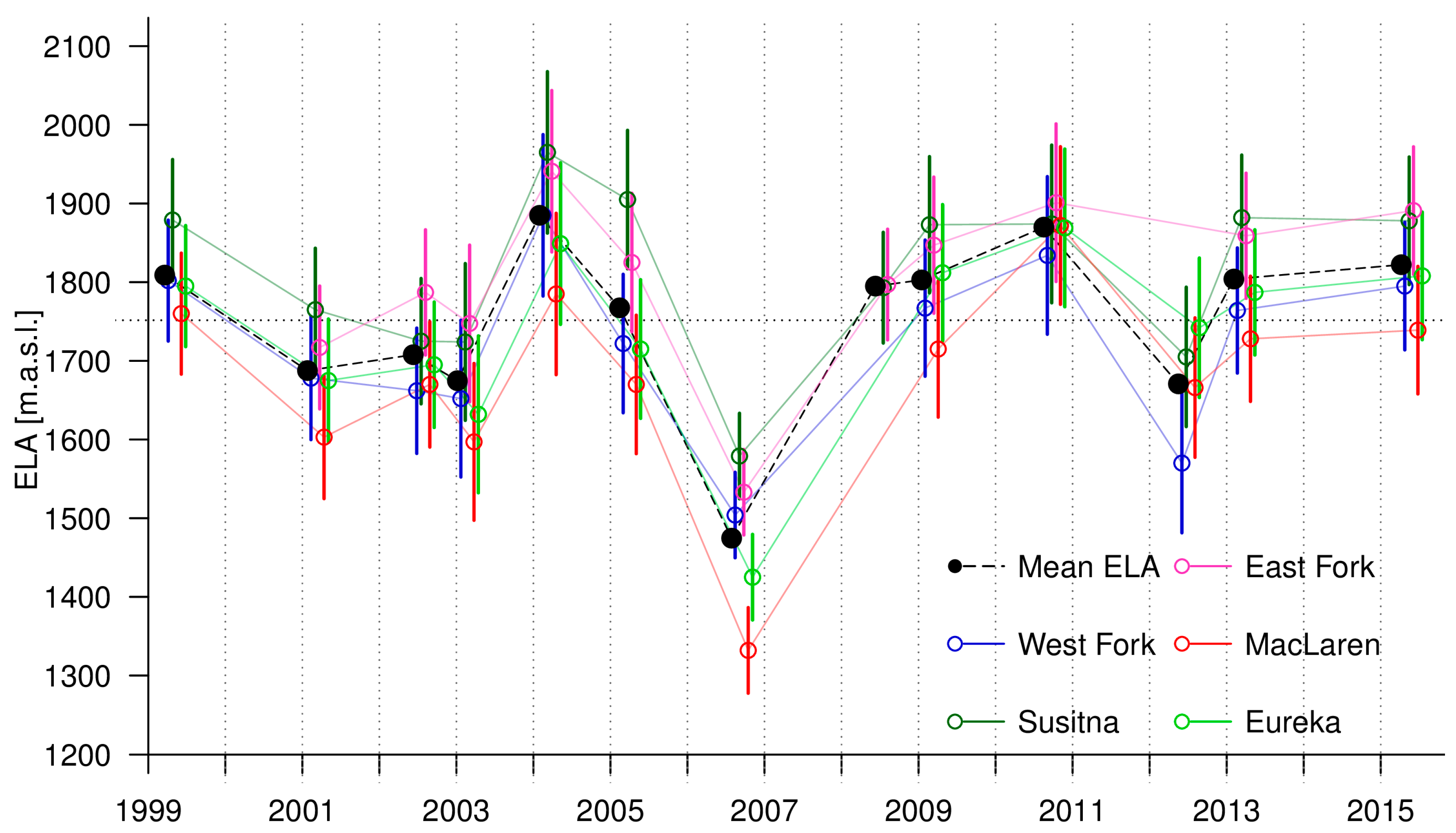
The annual ELAs (± uncertainty) for the five largest glaciers ranged from 1332 ± 25 m a.s.l. (MacLaren, 2006) to 1965 ± 100 m a.s.l. (Susitna Glacier, 2004). Averaged over the period 1999–2015, these glaciers’ ELAs varied between roughly 1700 and 1800 m a.s.l. (Table 4), with a mean of 1745 ± 88 m a.s.l. (arithmetic mean of the five largest glaciers). The inter-annual variability of the ELAs is illustrated in Figure 6. Most glaciers have their maximum ELA in 2004, except for MacLaren and Eureka Glaciers, which show their maximum in 2010. The ELAs in 2004 are high, although the observations were made relatively early in the melt season, indicating that the ELAs probably represent lower bounds. All glaciers have their minimum ELA in 2006, when the differences between the glaciers are also the largest. We also find the lowest uncertainties in 2006 because ELAs are located in low-lying regions, which tend to be less steep. Consistent with the pattern of ELA, West Fork shows the smallest mean AAR (46%), while MacLaren has the highest AAR (60%, Table 4).
A time series of the annual ELA estimates is shown in Figure 6. We conducted a linear trend analysis, but for all glaciers, the trend is not significant at the 95% confidence interval. Detecting a trend is difficult due to the relatively short observation period (17 years with three years missing), combined with large interannual variability. Trend analysis is further hampered by the fact that observations span over a period of three months and therefore, not all observations represent annual ELAs (i.e., refer to the end of each year’s melt season). Most ELA observations were made at the beginning of August, i.e., before the end of the melt season, and ELAs are expected to rise further as the melt season proceeds. These ELAs thus correspond to lower bound estimates.
We performed a rough back on the envelope calculation to provide an indication of how much the annual ELAs are underestimated. We calculated the rates of increase in ELA for each of the five glaciers for the three years for which multiple ELAs could be determined between mid-July and the end of the melt season (13 July–16 September 1999, 12 July–16 September 2004, 20 June–16 September 2005). We assumed that 16 September marked the end of the ablation season [2]. The rates were similar among all glaciers for the period between 12–13 July and the end of the season date for 1999 and 2004 (3.1 m day−1 0 ± 0.7). The mean rate was considerably higher for all glaciers in 2005 (8.3 m day−1 ± 2.1). Annual ELAs were computed using the lower mean rate, as all ELAs were derived after 12–13 July. The results indicate that the annual ELAs are underestimated by 82 ± 19 m a.s.l. averaged over all 14 years and glaciers with a maximum of 185 m a.s.l. for Eureka Glacier in 2003, but they must be interpreted with caution given the simplicity of the approach.
6. Discussion
6.1. Comparison with Other Studies
Our results are in agreement with other mass balance studies in Alaska. Increasing mass losses and thinning rates of Alaskan glaciers since the mid-1990s have been described, for example, by [1,2,43]. Clarke, et al. [44] calculated a mean thinning rate for the Susitna basin of 0.3 m yr−1 for the time interval 1949–1982. We found a slightly higher rate of 0.41 ± 0.07 m yr−1 for the interval 1951–2005. For Susitna Glacier, Larsen, et al. [3] observed a thinning rate of 0.86 m yr−1 for the interval 1993–2013, which is close to our study’s 0.91 ± 0.48 m yr−1 for the interval 2005–2010. In the same study, MacLaren Glacier was found to thin by a rate of 0.7 m yr−1 during the interval 1995–2013, which again is close to this study’s rate of 0.84 ± 0.90 m yr−1 for the interval 2005–2010. For East Fork Glacier, Arendt, et al. [1] calculated a thinning rate of 0.32 ± 0.06 m yr−1 for the period (1950–1995), which is larger than what we found for the period 1951–2005 (−0.23 ± 0.28 m yr−1), but is within the estimated error.
6.2. ELA and AAR
The highest ELAs occur during the extraordinarily warm summer in 2004, while the lowest mean ELA in 2006 coincides with a colder than average summer [45]. The annual ELAs did not show a statistically significant trend, which might be due to the limited length of the ELA time series and large interannual variability. The major limiting factor for the availability of adequate satellite data was the long recurring interval of the Landsat satellites (one to two weeks) and frequently occurring cloud cover.
Previous studies have found a strong relationship between ELA, AAR, and mass balance (e.g., [46]); thus, ELA and AAR are direct indicators for a glacier’s health. A rising ELA is associated with decreasing AAR as a glacier adapts to new climatic conditions. We have, however, no knowledge of the steady state AAR of our study glaciers, which complicates the interpretation of AAR values. Typically steady-state AARs range between 0.5 and 0.6 [27,46]. The mean AARs for the five largest glaciers are roughly within this range (46% and 63% over the period 1999–2005), thus providing no indication for the glaciers’ imbalance. However, the AARs for all glaciers are probably lower bounds, since, for several years, the values were derived before the end of the melt season (Table 5, Appendix A). Nevertheless, our results provide useful information for validation in future modeling efforts.
6.3. Surge Effects
West Fork Glacier is known to have surged in 1935 and again in 1987–1988 [18]. Hence, the NED DEM (1951) and the ASTER DEM (2005) were both acquired roughly 16 years after a surge had occurred. Assuming that the recurrence interval has not changed, the DEMs should reflect a similar surge state and therefore, the observed elevations changes almost exclusively reflect climatic change. During the period 2005–2010, West Fork Glacier experienced strongly accelerated mass loss (Table 3). The glacier underwent a surge in 1987–1988 and is now in its quiescent phase. Thus, the ice, brought downwards by the surge, can be expected to waste away more rapidly [47]. However, similar accelerations are also seen at the other glaciers in the basin, pointing to climate change as the primary driver of the glacier’s acceleration of thinning compared to the earlier period, subduing any surge-related effects.
Susitna Glacier last surged in 1951. Although the maps’ exact dates vary between 1948 and 1954 and are not known for the glacier, an analysis of moraine patterns indicate that the NED DEM reflects the glacier’s immediate post-surge state. In contrast, the 2005 ASTER DEM and the 2010 IfSAR DEM reflect the glacier’s pre-surge state, assuming a surge recurrence interval of 50–60 years [18]. As significant mass is transported during a surge from the reservoir area (typically in the accumulation area) to the receiving area in the ablation zone, the NED DEM will include lower elevations in the former area and higher elevations in the latter area compared to the immediate pre-surge state. Hence, assuming no climate change, one would expect a thickening in the reservoir area and a strong thinning in the ablation area after the surge. Therefore, more thickening or less thinning can be expected in the reservoir area and higher thinning in the ablation area during the period 1951–2010 compared to neighboring non-surging glaciers with a similar morphology and climate conditions. However, Figure 4c indicates that Susitna Glacier experienced lower thinning rates than West Fork Glacier in the ablation area.
In the period 2005–2010, Susitna Glacier shows spatially coherent thickening rates up to 5 m yr−1 in tributary C, although the area is not very steep (4–8, Figure 1 and Figure 3). However, in situ mass-balance measurements and observations of extensive wind erosion in the tributaries C [9] suggest that such a thickening is unrealistic, and is most likely due to DEM errors rather than a surge build-up. Similarly spatially coherent thickening is found in tributary D, but the area is very steep and therefore, the thickening is also due to DEM errors.
The main trunk shows pronounced thinning over large parts (especially between 9 and 14 km upglacier from the terminus at approximately 900–1150 m a.s.l.). The thinning rates are considerably higher at Susitna Glacier than at similar elevations on West Fork Glacier, although the former area is heavily debris-covered, while the latter is largely debris-free (Figure 1). Thinning rates are affected by debris cover; debris cover of more than a few cm typically isolates the underlying ice and leads to substantially lower ablation rates [2], although recent studies have found substantial thinning rates on some heavily debris-covered glacier tongues [48]. Susitna Glacier is debris-covered over large parts of its ablation area and elevation changes near the terminus (0 to ~6 km) over the period 1951–2010 are close to zero (Figure 3). This may be a consequence of Susitna’s surge in 1951/52. This region is beyond the advance of the surge and was therefore not affected by high mass inputs due to the surge [17]. Thus, the area might be thickly covered in debris, causing thinning rates to be small. It is also possible that the area is affected by erroneous values in the NED DEM, similar to West Fork Glacier’s tributary B (see chapter 5.2), since, during the period 2005–2010 (differencing the IfSAR from the ASTER DEM), such a pattern is missing.
Overall, given the uncertainties in our DEMs, our analysis does not allow us to unambiguously interpret the observed thickness changes in terms of surge behavior. However, unlike on neighboring Black Rapids Glacier [23,47], surges over the next decades cannot be ruled out based on our analysis. A surge would not only alter the glaciers’ morphology but also lead to considerable increases in the sediment input into the Susitna River.
7. Conclusions
Despite uncertainties inherent to the ASTER DEM and the NED DEM, our analysis indicates that the glaciers in the Susitna basin have experienced substantial retreat, thinning, and mass loss between 1951 and 2010. The thinning rates almost tripled from 0.41 ± 0.07 m yr−1 in 1951–2005, to 1.20 ± 0.25 m yr−1 in 2005–2010. The accelerated mass loss indicates that the glaciers have not yet adapted to the current climate, although the average AAR of 56 ± 11% is within the range of AAR values typically assumed for steady-state conditions. The recent acceleration of mass loss is probably a response to the pronounced warming trend which has occurred since the middle of the 20th century [7,49]. All glaciers show regions of thickening in the accumulation area between 1951–2005 and 2005–2010, most likely due to errors in the DEM. Uncertainties in the DEMs and surge behavior of some glaciers not being well-known complicate the interpretation of the elevation change patterns. However, the consistency of loss in area and thickness over all investigated glaciers, despite pronounced surges on West Fork in 1987–1988 and Susitna Glacier in 1951–1952, suggests that climatic effects dominate the glacier’s mass changes, subduing any feedback due to surge behavior. The consistency of the accelerated mass and area changes across the study region suggests that climate change is the dominant driver of the observed thickness changes and their spatial distribution.
The mean ELA over the period 1999 to 2015 is 1745 ± 88 m a.s.l., without a significant trend of annual ELAs over time. Using the end of summer snow line as a proxy for the estimation of the annual ELA proved to be difficult in some years due to the lack of suitable Landsat data close to the end of melt season. Nevertheless, our results present the first measurements of the ELA in this region. Although in some years the data are a lower bound, they provide useful information for validation in modeling efforts.
Our results provide valuable data for mass balance modeling studies, but should be complemented with additional mass balance data resolving annual or seasonal variations.
Acknowledgments
R.W. was financially supported by a PROMOS scholarship to support an internship at Univ. Alaska Fairbanks during which this study was initiated. The publishing of this paper was financially supported by the FAU open access fund provided through the German Research Foundation (DFG). R.H. acknowledges funding from the Alaska Energy Authority.
Author Contributions
R.W. performed the data analyses. C.K. supported the data analysis by providing code and a methodological framework. R.H. and M.B. jointly supervised the work. R.W., R.H., and M.B. wrote the manuscript. All authors revised the manuscript.
Conflicts of Interest
The authors declare no conflict of interest.
Appendix A

Table A1.
Characteristics of the Landsat images used to estimate the ELA.
| Sensor | Date Acquired | Product ID |
|---|---|---|
| Landsat 7 ETM+ | 16 August 1999 | LE70680161999228AGS00 |
| Landsat 7 ETM+ | 05 August 2001 | LE70680162001217AGS00 |
| Landsat 7 ETM+ | 02 September 2002 | LE70670162002245EDC01 |
| Landsat 7 ETM+ | 19 July 2003 | LE70670162003200EDC01 |
| Landsat 5 TM | 10 August 2003 | LT50690152003222PAC02 |
| Landsat 7 ETM+ | 06 August 2004 | LE70670162004219EDC01 |
| Landsat 7 ETM+ | 09 August 2005 | LE70670162005221EDC00 |
| Landsat 5 TM | 12 September 2006 | LT50680162006255PAC01 |
| Landsat 7 ETM+ | 02 September 2008 | LE70670162008246EDC00 |
| Landsat 5 TM | 03 August 2009 | LT50680162009215GLC00 |
| Landsat 5 TM | 16 September 2010 | LT50670162010259GLC00 |
| Landsat 7 ETM+ | 28 August 2012 | LE70670162012241EDC00 |
| Landsat 8 OLI | 07 August 2013 | LC80670162013219LGN00 |
| Landsat 8 OLI | 20 August 2015 | LC80680162015232LGN00 |
References
- Arendt, A.A.; Echelmeyer, K.A.; Harrison, W.D.; Lingle, C.S.; Valentine, V.B. Rapid wastage of Alaska glaciers and their contribution to rising sea level. Science 2002, 297, 382–386. [Google Scholar] [CrossRef] [PubMed]
- Berthier, E.; Schiefer, E.; Clarke, G.K.C.; Menounos, B.; Rémy, F. Contribution of Alaskan glaciers to sea-level rise derived from satellite imagery. Nat. Geosci. 2010, 3, 92–95. [Google Scholar] [CrossRef]
- Larsen, C.F.; Burgess, E.; Arendt, A.A.; O’Neel, S.; Johnson, A.J.; Kienholz, C. Surface melt dominates Alaska glacier mass balance. Geophys. Res. Lett. 2015, 42, 5902–5908. [Google Scholar] [CrossRef]
- Gardner, A.S.; Moholdt, G.; Cogley, J.G.; Wouters, B.; Arendt, A.A.; Wahr, J.; Berthier, E.; Hock, R.; Pfeffer, W.T.; Kaser, G.; et al. A reconciled estimate of glacier contributions to sea level rise: 2003 to 2009. Science 2013, 340, 852–857. [Google Scholar] [CrossRef] [PubMed]
- Das, I.; Hock, R.; Berthier, E.; Lingle, C.S. 21st-century increase in glacier mass loss in the Wrangell Mountains, Alaska, USA, from airborne laser altimetry and satellite stereo imagery. J. Glaciol. 2014, 60, 283–293. [Google Scholar] [CrossRef]
- Johnson, A.J.; Larsen, C.F.; Murphy, N.; Arendt, A.A.; Zirnheld, S.L. Mass balance in the Glacier Bay area of Alaska, USA, and British Columbia, Canada, 1995–2011, using airborne laser altimetry. J. Glaciol. 2013, 59, 632–648. [Google Scholar] [CrossRef]
- Shulski, M.; Wendler, G. The Climate of Alaska; University of Alaska Press: Fairbanks, AK, USA, 2007. [Google Scholar]
- Loso, M.; Arendt, A.A.; Larsen, C.; Rich, J.; Murphy, N. Alaskan National Park Glaciers-Status and Trends: Final Report; National Park Service: Fort Collins, CO, USA, 2014. [Google Scholar]
- Wolken, G.; Bliss, A.; Hock, R.; Whorton, E.; Braun, J.; Liljedahl, A.; Zhang, J.; Youcha, E.; Schulla, J.; Gusmeroli, A.; et al. Susitna-Watana Hydroelectric Project (FERC No. 14241) Glacier and Runoff Changes Study, Final Study Report; Alaska Energy Authority: Anchorage, AK, USA, 2015. [Google Scholar]
- Clarke, T.S.; Johnson, D.; Harrison, W.D. Glacier Mass Balances and Runoff in the Upper Susitna and Maclaren River Basins, 1981–1983. Available online: http://www.arlis.org/docs/vol1/Susitna/27/APA2781.pdf (accessed on 18 March 2017).
- Harrison, W.D.; Drage, B.T.; Bredthauer, S.; Johnson, D.; Schoch, C.; Follett, A.B. Reconnaissance of the glaciers of the Susitna River basin in connection with proposed hydroelectric development. Ann. Glaciol. 1983, 4. [Google Scholar] [CrossRef]
- Benn, D.I.; Lehmkuhl, F. Mass balance and equilibrium-line altitudes of glaciers in high-mountain environments. Quat. Int. 2000, 65–66, 15–29. [Google Scholar] [CrossRef]
- Clare, G.R.; Fitzharris, B.B.; Chinn, T.J.H.; Salinger, M.J. Interannual variation in end-of-summer snowlines of the Southern Alps of New Zealand, and relationships with Southern Hemisphere atmospheric circulation and sea surface temperature patterns. Int. J. Climatol. 2002, 22, 107–120. [Google Scholar] [CrossRef]
- Rabatel, A.; Letréguilly, A.; Dedieu, J.-P.; Eckert, N. Changes in glacier equilibrium-line altitude in the western Alps from 1984 to 2010: Evaluation by remote sensing and modeling of the morpho-topographic and climate controls. Cryosphere 2013, 7, 1455–1471. [Google Scholar] [CrossRef]
- Brabets, T. Precipitation Map of Alaska; USGS: Reston, VA, USA, 1997. Available online: https://agdc.usgs.gov/data/usgs/water/metadata/ak_precip.html (accessed on 18 March 2017).
- Post, A. Distribution of surging glaciers in western North America. J. Glaciol. 1969, 8, 229–240. [Google Scholar] [CrossRef]
- Meier, M.F.; Post, A. What are glacier surges? Can. J. Earth. Sci. 1969, 6, 807–817. [Google Scholar] [CrossRef]
- Clarke, T.S. Glacier dynamics in the Susitna River basin, Alaska, U.S.A. J. Glaciol. 1991, 37, 97–106. [Google Scholar] [CrossRef]
- Herreid, S.; Truffer, M. Automated detection of unstable glacier flow and a spectrum of speed-up behavior in the Alaska Range. J. Geophys. Res. Earth. Surf. 2016, 121, 64–81. [Google Scholar] [CrossRef]
- Kienholz, C.; Herreid, S.; Rich, J.L.; Arendt, A.A.; Hock, R.; Burgess, E.W. Derivation and analysis of a complete modern-date glacier inventory for Alaska and northwest Canada. J. Glaciol. 2015, 61, 403–420. [Google Scholar] [CrossRef]
- Pfeffer, W.T.; Arendt, A.A.; Bliss, A.; Bolch, T.; Cogley, J.G.; Gardner, A.S.; Hagen, J.-O.; Hock, R.; Kaser, G.; Kienholz, C.; et al. The Randolph Glacier inventory: A globally complete inventory of glaciers. J. Glaciol. 2014, 60, 537–552. [Google Scholar] [CrossRef]
- Manley, W.F. Geospatial inventory and analysis of glaciers: A case study for the Eastern Alaska range. In Satellite Image Atlas of Glaciers of the World: Alaska; Unites States Government Printing Office: Washington, DC, USA, 2008. [Google Scholar]
- Kienholz, C.; Hock, R.; Truffer, M.; Arendt, A.A.; Arko, S. Geodetic mass balance of surge-type Black Rapids Glacier, Alaska, 1980–2001–2010, including role of rockslide deposition and earthquake displacement. J. Geophys. Res. Earth Surf. 2016, 121, 2358–2380. [Google Scholar] [CrossRef]
- Nuth, C.; Kääb, A. Co-registration and bias corrections of satellite elevation data sets for quantifying glacier thickness change. Cryosphere 2011, 5, 271–290. [Google Scholar] [CrossRef]
- Huss, M. Density assumptions for converting geodetic glacier volume change to mass change. Cryosphere 2013, 7, 877–887. [Google Scholar] [CrossRef]
- Chinn, T.J.H. Glacier fluctuations in the Southern Alps of New Zealand determined from SNOWLINE elevations. Arct. Antarct. Alp Res. 1995, 27, 187–198. [Google Scholar] [CrossRef]
- Chinn, T.J.H.; Salinger, M.J. New Zealand Glacier Snowline Survey. Available online: https://sirgnz.files.wordpress.com/2014/09/snowline-survey-1999-chinn.pdf (accessed on 18 March 2017).
- Wu, Y.; He, J.; Guo, Z.; Chen, A. Limitations in identifying the equilibrium-line altitude from the optical remote-sensing derived snowline in the Tien Shan, China. J. Glaciol. 2014, 60, 1093–1100. [Google Scholar] [CrossRef]
- Ziemen, F.A.; Hock, R.; Aschwanden, A.; Khroulev, C.; Kienholz, C.; Melkonian, A.K.; Zhang, J. Modeling the evolution of the Juneau Icefield between 1971 and 2100 using the Parallel Ice Sheet Model (PISM). J. Glaciol. 2016, 62, 199–214. [Google Scholar] [CrossRef]
- Geographic Information Network of Alaska 2012. Alaska IfSAR Digital Elevation Model (DEM) Data: Alaska IfSAR DEM Data hosted by GINA. Available online: http://ifsar.gina.alaska.edu (accessed on 17 December 2016).
- Toutin, T. 3D Topographic mapping with ASTER Stereo Data in Rugged Topography. IEEE Trans Geosci Remote Sens 2002, 40, 2241–2247. [Google Scholar] [CrossRef]
- Mercer, B. Combining LIDAR and IfSAR: What can you expect? Procceedings of the Photogrammetric Week, Stuttgart, Germany, 5–9 September 2001. [Google Scholar]
- Wingham, D.; Shepherd, A.; Muir, A.; Marshall, G. Mass balance of the Antarctic ice sheet. Philos. Trans. R. Soc. Lond. A 2006, 364, 1627–1635. [Google Scholar] [CrossRef] [PubMed]
- Ridley, J.K.; Partington, K.C. A model of satellite radar altimeter return from ice sheets. Int. J. Remote Sens. 2007, 9, 601–624. [Google Scholar] [CrossRef]
- Zemp, M.; Thibert, E.; Huss, M.; Stumm, D.; Rolstad Denby, C.; Nuth, C.; Nussbaumer, S.U.; Moholdt, G.; Mercer, A.; Mayer, C.; et al. Reanalysing glacier mass balance measurement series. Cryosphere 2013, 7, 1227–1245. [Google Scholar] [CrossRef]
- Ruiz, L.; Berthier, E.; Viale, M.; Pitte, P.; Masiokas, M. Recent geodetic mass balance of Monte Tronador glaciers, North Patagonian Andes. Cryosphere Discuss. 2017, 11. [Google Scholar] [CrossRef]
- Bretherton, C.S.; Widmann, M.; Dymnikov, V.P.; Wallace, J.M.; Bladé, I. The effective number of spatial degrees of freedom of a time-varying field. J. Climate 1999, 12, 1990–2009. [Google Scholar] [CrossRef]
- Schiefer, E.; Menounos, B.; Wheate, R. Recent volume loss of British Columbian glaciers, Canada. Geophys. Res. Lett. 2007, 34, 1–6. [Google Scholar] [CrossRef]
- DeBeer, C.M.; Sharp, M.J. Recent changes in glacier area and volume within the southern Canadian Cordillera. Ann. Glaciol. 2007, 46, 215–221. [Google Scholar] [CrossRef]
- Harrison, W.D.; Echelmayer, K.A.; Chacho, E.F.; Raymond, C.F.; Benedict, R.J. The 1987-88 surge of West Fork Glacier, Susitna Basin, Alaska, U.S.A. J. Glaciol. 1994, 40, 241–254. [Google Scholar] [CrossRef]
- Kirkbride, M.P. The temporal significance of transitions from melting to calving termini at glaciers in the central Southern Alps of New Zealand. Holocene 1993, 3, 232–240. [Google Scholar] [CrossRef]
- Sugiyama, S.; Minowa, M.; Sakakibara, D.; Skvarca, P.; Sawagaki, T.; Ohashi, Y.; Naito, N.; Chikita, K. Thermal structure of proglacial lakes in Patagonia. J. Geophys. Res. Earth Surf. 2016, 121, 2270–2286. [Google Scholar] [CrossRef]
- Larsen, C.F.; Motyka, R.J.; Arendt, A.A.; Echelmeyer, K.A.; Geissler, P.E. Glacier changes in southeast Alaska and northwest British Columbia and contribution to sea level rise. J. Geophys. Res. 2007, 112. [Google Scholar] [CrossRef]
- Clarke, T.S.; Johnson, D.; Harrison, W.D. Some Aspects of Glacier Hydrology in the Upper Susitna and Maclaren River Basins, Alaska. Available online: http://www.arlis.org/docs/vol1/Susitna/41/APA4159.pdf (accessed on 18 March 2017).
- Arendt, A.A.; Luthcke, S.; Gardner, A.; O’Neel, S.R.; Hill, D.; Moholdt, G.; Abdalati, W. Analysis of a GRACE global mascon solution for Gulf of Alaska glaciers. J. Glaciol. 2013, 59, 913–924. [Google Scholar] [CrossRef]
- Dyurgerov, M.B.; Meier, M.F.; Bahr, D.B. A new index of glacier area change: A tool for glacier monitoring. J. Glaciol. 2009, 55, 710–716. [Google Scholar] [CrossRef]
- Shugar, D.H.; Rabus, B.T.; Clague, J.J. Elevation changes (1949–1995) of Black Rapids Glacier, Alaska, derived from a multi-baseline InSAR DEM and historical maps. J. Glaciol. 2010, 56, 625–634. [Google Scholar] [CrossRef]
- Gardelle, J.; Berthier, E.; Arnaud, Y.; Kääb, A. Region-wide glacier mass balances over the Pamir-Karakoram-Himalaya during 1999–2011. Cryosphere 2013, 7, 1263–1286. [Google Scholar] [CrossRef]
- Arendt, A.A.; Walsh, J.E.; Harrison, W.D. Changes of glaciers and climate in northwestern North America during the late twentieth century. J. Climate 2009, 22, 4117–4134. [Google Scholar] [CrossRef]
Figure 1.
Map of studied glaciers in the Susitna River basin. The five largest named glaciers are marked in dark grey and the remaining glacierized area in light grey. Debris covered ice is shown in brown. Glacier outlines and debris cover extent are derived from 2010 Landsat imagery. Tributaries discussed in the text are labeled with letters. Contour lines for altitudes of 1000, 1500, 2000, and 2500 m a.s.l. are added. The irregular course of the 1000 m contour on West Fork and Susitna Glacier reflects the hummocky surface topography caused by debris cover.
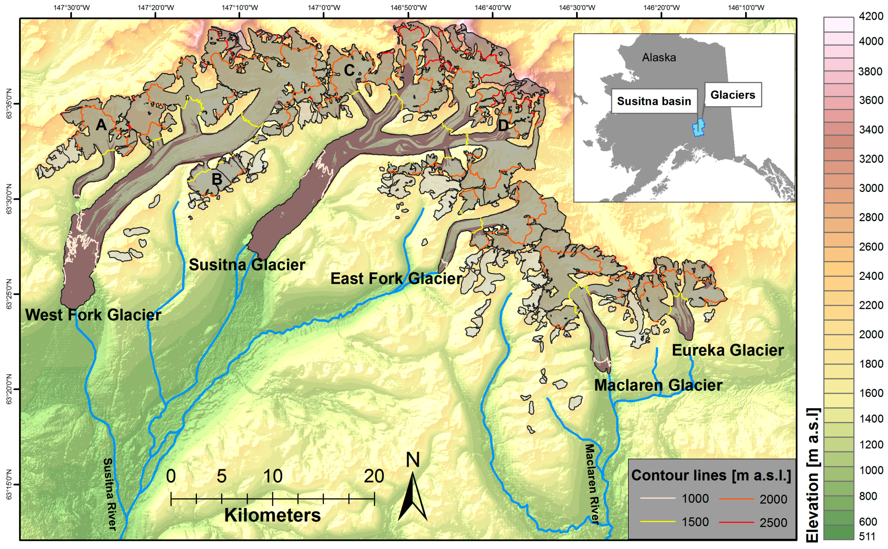
Figure 2.
Frequency distribution of elevation changes dh over the periods (a) 1951–2010 (NED-IfSAR); (b) 1951–2005 (NED-ASTER); and (c) 2005–2010 (ASTER-IfSAR) across ice-free terrain before and after the corrections (yellow, green, and red), and over the glacierized area (blue). Bin size is 1 m.
Figure 2.
Frequency distribution of elevation changes dh over the periods (a) 1951–2010 (NED-IfSAR); (b) 1951–2005 (NED-ASTER); and (c) 2005–2010 (ASTER-IfSAR) across ice-free terrain before and after the corrections (yellow, green, and red), and over the glacierized area (blue). Bin size is 1 m.
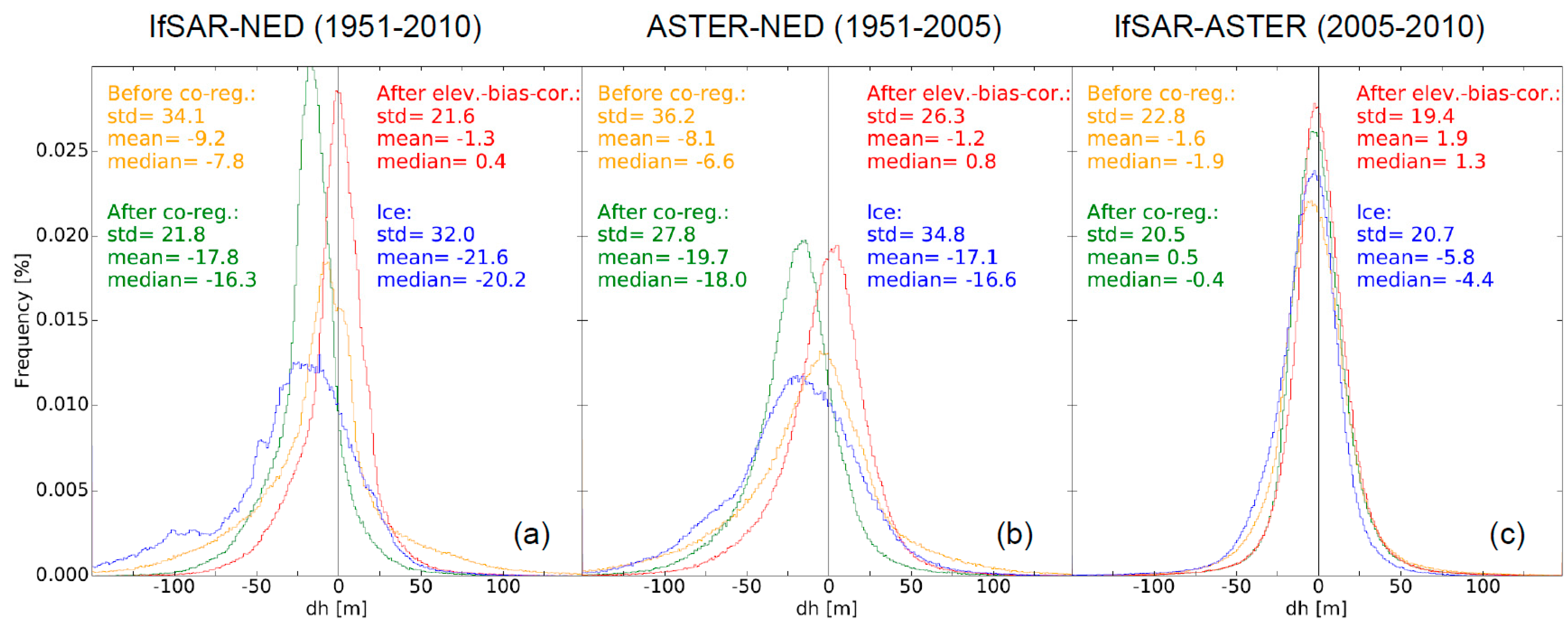
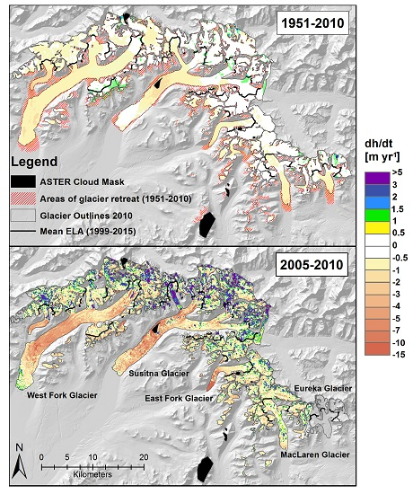
Figure 3.
Spatially distributed elevation changes [m yr−1] for the study periods (a) 1951–2010 and (b) 2005–2010. Hatched areas represent areas that became ice-free between 1951 and 2010 due to glacier retreat. Black areas represent the cloud error mask for the ASTER DEM. The mean equilibrium line for the years 1999–2015 is shown with black solid lines. Note that no elevation changes 2005–2010 are available for Eureka Glacier since the ASTER DEM does not cover the entire glacier.
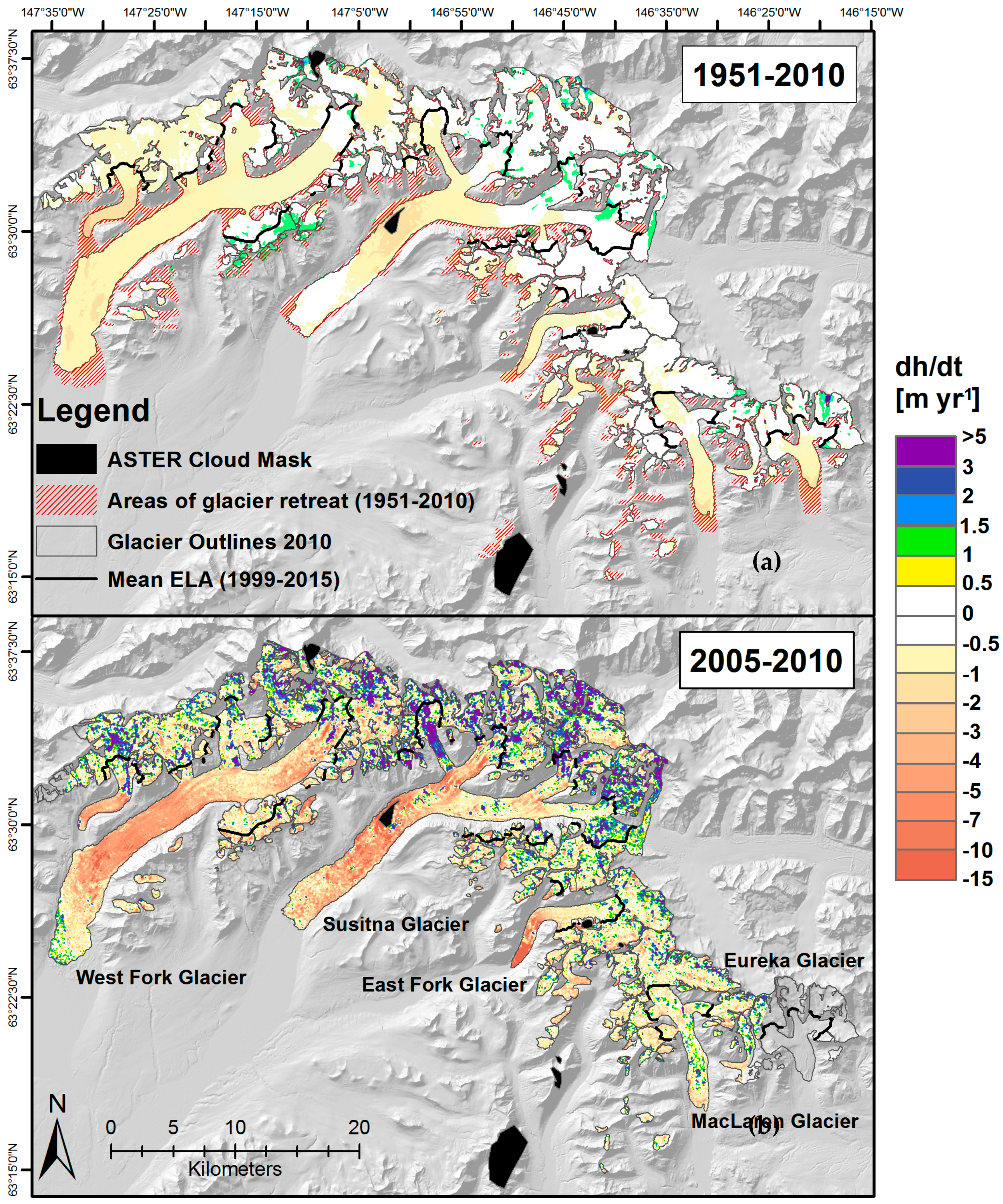
Figure 4.
Glacier hypsometry in 50 m elevation bins for (a) 1951 and (b) 2010 and altitude-dependent mean elevation change rates dh/dt for (c) 1951–2005, (d) 2005–2010, and (e) 1951–2010. dh/dt values are averaged over all pixels of 50 m elevation bin. Area and elevation values in (a) and (b) are based on the glacier outlines and DEMs of the corresponding years.
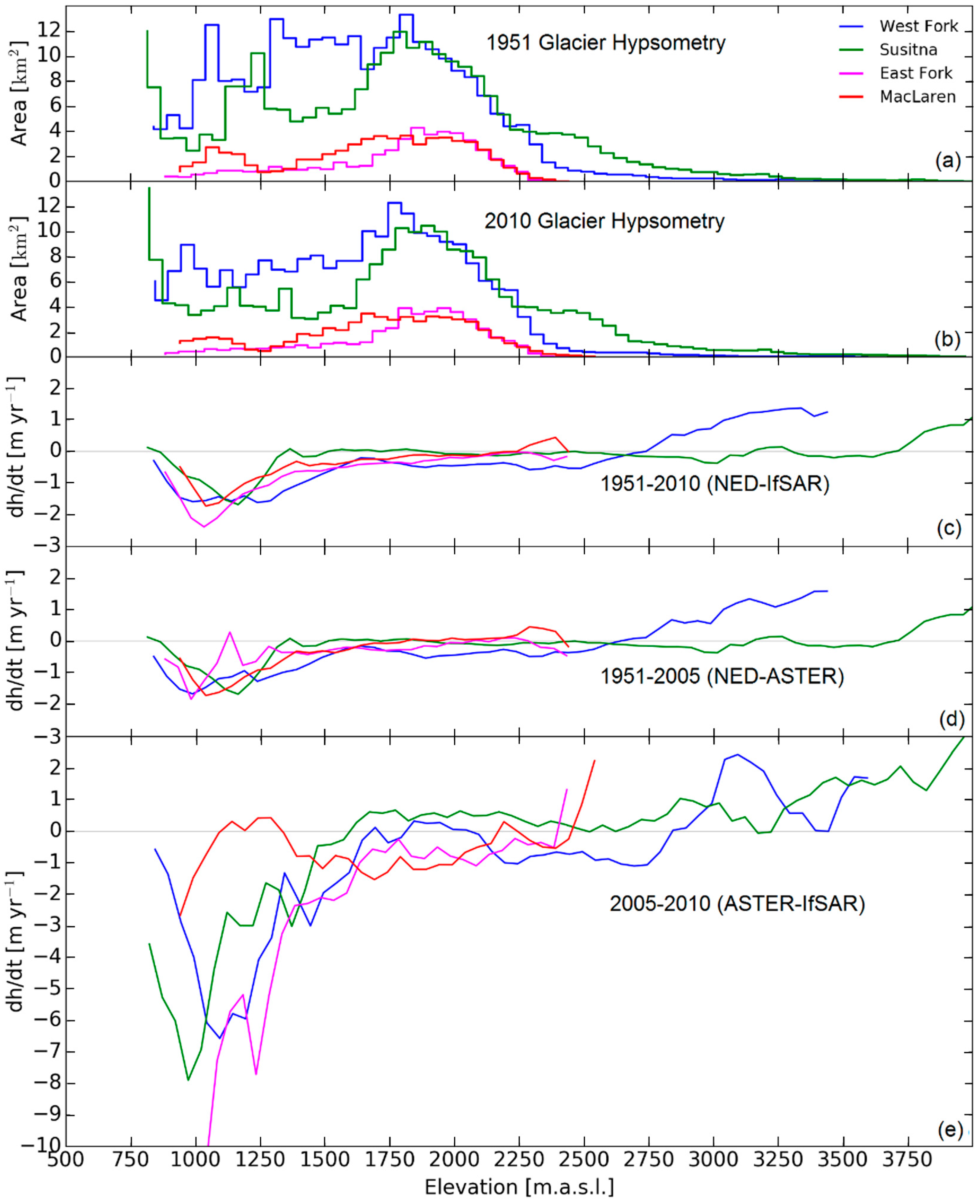
Figure 5.
Slope map of the studied glaciers in the Susitna River basin. Slope values [°] were calculated using ArcGIS based on the IfSAR DEM. Glacier outlines of 2010 are shown in black.
Figure 5.
Slope map of the studied glaciers in the Susitna River basin. Slope values [°] were calculated using ArcGIS based on the IfSAR DEM. Glacier outlines of 2010 are shown in black.

Figure 6.
Time series (1999–2015) of annual ELAs for the five largest glaciers. The mean ELA refers to the average of the five glaciers’ annual ELAs. Vertical lines show the uncertainties. For each year, the x-axis refers to the period 1 August to 15 October. For the year 2003, the date was set to 1 August, which lies in between the acquisition date of the two Landsat scenes that were used. The mean ELA of all glaciers (black dots) is positioned to coincide with the date, which the ELA refers to, while for better readability each individual glacier’s ELA is slightly offset. The black dotted line marks the time-averaged ELA of the five large glaciers (1761 m a.s.l.).

Table 1.
Overview of geospatial data sets used in this study and derived products. dh denotes surface elevation change.
Table 1.
Overview of geospatial data sets used in this study and derived products. dh denotes surface elevation change.
| Data | Spatial Resolution | Date | Product | Source |
|---|---|---|---|---|
| Landsat 5–8 | 30 m | 1999–2015 | ELA; AAR | NASA Landsat Program |
| ASTER DEM 1; | 30 m | 9 August 2005 | dh | NASA Land Processes Distributed Active Archive Center (LP DAAC) |
| National Elevation Dataset (NED) | 40 m | ~1951 | dh | USGS |
| IfSAR DEM | 30 m | 19/20 June 2010 | dh | Intermap Technologies |
| Topographic map quadrangles 2: | - | ~1951 | Outlines | USGS |
| Randolph Glacier Inventory v.5.0 | - | 2010 | Outlines | [20] |
1. The ASTER granule IDs used to compute the ASTER DEMs are ASTL1A0508092117490508120579 and ASTL1A0508092117400508120578.
2. The quadrangles’s reference numbers are Mt. Hayes B-5/6 & C-6, Healy B-1/2 & C-1/2.
Table 2.
Glacier area and terminus elevation in 1951 and 2010 and the area change between 1951–2010 for the five largest glaciers and all glaciers in the Susitna basin. Glaciers termed as “Others” include all unnamed, smaller glaciers (shaded in light grey in Figure 1). Terminus elevations were extracted from the corresponding DEMs.
| Area | Area change | Terminus | ||||
|---|---|---|---|---|---|---|
| Glacier | 1951 [km²] | 2010 [km²] | [km²] | [%] | 1951 [m a.s.l.] | 2010 [m a.s.l.] |
| West Fork | 268 | 233 | −35 ± 4 | −13 ± 1 | 839 | 844 |
| Susitna | 244 | 220 | −24 ± 3 | −10 ± 1 | 815 | 822 |
| East Fork | 46 | 44 | −2 ± 0 | −4 ± 0 | 884 | 884 |
| MacLaren | 59 | 56 | −3 ± 0 | −5 ± 0 | 940 | 942 |
| Eureka | 39 | 34 | −5 ± 1 | −13 ± 3 | 1115 | |
| Others | 138 | 81 | −58 ± 7 | −42 ± 5 | − | − |
| All | 796 | 668 | −128 ± 15 | −16 ± 2 | − | − |
Table 3.
Glacier-wide elevation (dh/dt) and mass changes (dM/dt) over two periods: 1951–2005 (NED-ASTER), 2005–2010 (ASTER-IfSAR), and 1951–2010 (NED-IfSAR). Data for Eureka Glacier (EG) is missing for the periods 1951–2005 and 2005–2010 due to the lack of ASTER DEM coverage. dM is given in megatons. Note that dh values refer to ice equivalent.
| 1951–2005 | 2005–2010 | 1951–2010 | ||||
|---|---|---|---|---|---|---|
| Glacier | dh/dt [m yr−1] | dM/dt [Mt yr−1] | dh/dt [m yr−1] | dM/dt [Mt yr−1] | dh/dt [m yr−1] | dM/dt [Mt yr−1] |
| West Fork | −0.70 ± 0.12 | −0.15 ± 0.03 | −1.61 ± 0.43 | −0.32 ± 0.10 | −0.76 ± 0.13 | −0.16 ± 0.03 |
| Susitna | −0.22 ± 0.13 | −0.05 ± 0.03 | −0.91 ± 0.48 | −0.17 ± 0.12 | −0.30 ± 0.13 | −0.07 ± 0.03 |
| East Fork | −0.23 ± 0.28 | −0.01 ± 0.01 | −1.64 ± 1.02 | −0.06 ± 0.04 | −0.44 ± 0.18 | −0.02 ± 0.01 |
| MacLaren | −0.34 ± 0.24 | −0.02 ± 0.01 | −0.84 ± 0.90 | −0.04 ± 0.05 | −0.40 ± 0.17 | −0.02 ± 0.01 |
| Eureka | − | − | − | − | −0.34 ± 0.18 | −0.01 ± 0.0 |
| Others | −0.23 ± 0.16 | −0.03 ± 0.02 | −0.96 ± 0.59 | −0.06 ± 0.07 | −0.48 ± 0.14 | −0.04 ± 0.02 |
| All | −0.41 ± 0.07 | −0.24 ± 0.05 | −1.20 ± 0.25 | −0.75 ± 0.17 | −0.48 ± 0.09 | −0.34 ± 0.05 |
Table 4.
Statistics of ELA and AAR analysis for the five large glaciers over the period 1999–2015. ELA and AAR values refer to the mean over the study period and N denotes the number of years with valid data. Values also include the standard deviation of the annual values as a measure of interannual variability. Maximum and mean ELA include the uncertainty based on Equation 2 and the corresponding year in bracket. EELA refers to the arithmetic mean of the annual ELA uncertainties. “All” refers to the arithmetic mean of the values (and uncertainties) of the five large glaciers.
| Glacier | ELA [m a.s.l.] | Max ELA [m a.s.l.] | Min ELA [m a.s.l.] | EELA [m .a.s.l.] | N | AAR [%] |
|---|---|---|---|---|---|---|
| West Fork | 1714 ± 88 | 1885 ± 111 (2004) | 1504 ± 123 (2006) | 92 | 13 | 46 ± 9 |
| Susitna | 1805 ± 93 | 1965 ± 100 (2004) | 1579 ± 71 (2006) | 90 | 14 | 53 ± 8 |
| East Fork | 1799 ± 91 | 1941 ± 128 (2004) | 1533 ± 81 (2006) | 95 | 12 | 63 ± 8 |
| MacLaren | 1672 ± 62 | 1872 ± 89 (2010) | 1332 ± 25 (2006) | 62 | 13 | 60 ± 9 |
| Eureka | 1734 ± 82 | 1869 ± 71 (2010) | 1425 ± 78 (2006) | 76 | 12 | 57 ± 11 |
| All | 1745 ± 88 | 1885 ± 95 (2004) | 1425 ± 74 (2006) | 81 | − | 56 ± 11 |
© 2017 by the authors. Licensee MDPI, Basel, Switzerland. This article is an open access article distributed under the terms and conditions of the Creative Commons Attribution (CC BY) license (http://creativecommons.org/licenses/by/4.0/).
Share and Cite
MDPI and ACS Style
Wastlhuber, R.; Hock, R.; Kienholz, C.; Braun, M. Glacier Changes in the Susitna Basin, Alaska, USA, (1951–2015) using GIS and Remote Sensing Methods. Remote Sens. 2017, 9, 478. https://doi.org/10.3390/rs9050478
AMA Style
Wastlhuber R, Hock R, Kienholz C, Braun M. Glacier Changes in the Susitna Basin, Alaska, USA, (1951–2015) using GIS and Remote Sensing Methods. Remote Sensing. 2017; 9(5):478. https://doi.org/10.3390/rs9050478
Chicago/Turabian StyleWastlhuber, Roland, Regine Hock, Christian Kienholz, and Matthias Braun. 2017. "Glacier Changes in the Susitna Basin, Alaska, USA, (1951–2015) using GIS and Remote Sensing Methods" Remote Sensing 9, no. 5: 478. https://doi.org/10.3390/rs9050478
Note that from the first issue of 2016, this journal uses article numbers instead of page numbers. See further details here.