A Machine Learning Method for Co-Registration and Individual Tree Matching of Forest Inventory and Airborne Laser Scanning Data

Abstract

Determining the exact position of a forest inventory plot—and hence the position of the sampled trees—is often hampered by a poor Global Navigation Satellite System (GNSS) signal quality beneath the forest canopy. Inaccurate geo-references hamper the performance of models that aim to retrieve useful information from spatially high remote sensing data (e.g., species classification or timber volume estimation). This restriction is even more severe on the level of individual trees. The objective of this study was to develop a post-processing strategy to improve the positional accuracy of GNSS-measured sample-plot centers and to develop a method to automatically match trees within a terrestrial sample plot to aerial detected trees. We propose a new method which uses a random forest classifier to estimate the matching probability of each terrestrial-reference and aerial detected tree pair, which gives the opportunity to assess the reliability of the results. We investigated 133 sample plots of the Third German National Forest Inventory (BWI, 2011–2012) within the German federal state of Rhineland-Palatinate. For training and objective validation, synthetic forest stands have been modeled using the Waldplaner 2.0 software. Our method has achieved an overall accuracy of 82.7% for co-registration and 89.1% for tree matching. With our method, 60% of the investigated plots could be successfully relocated. The probabilities provided by the algorithm are an objective indicator of the reliability of a specific result which could be incorporated into quantitative models to increase the performance of forest attribute estimations.

1. Introduction

Modeling and characterizing forest stands on small scales using high-resolution remote sensing data requires spatially explicit linking of inventory information and remote sensing data [1,2,3]. The exact sampling positions of field inventory plots are often determined using non-differential [4] or differential Global Navigation Satellite System (GNSS), which gives rise to location errors of up to several meters. In comparison, airborne laser scanning (ALS) provides absolute horizontal accuracies of about 25 cm (at 400 m flight altitude above ground) [5].

The effect of positional displacements between terrestrial reference data and ALS data has been investigated by Gobakken and Naesset [6] and Frazer et al. [7] at the sample plot level. They found that with increasing positional displacements the performance of biophysical models decreases in relation to the variable and stand characteristics. This problem exacerbates on individual tree level, since survey trees might get incorrectly linked to aerial detected trees (e.g., using ALS), which results in erroneous output data for further analyses.

Individual tree information has a specific added value for quantitative modeling compared to plot-based methods insofar as it includes features which address structural tree characteristics [8,9]. A general trend towards the usage of ALS data is recognizable [2]. Densities of about five to ten pulses per m² are sufficient for tree detection [10,11]. It has been shown that most methods perform well in the upper canopy layer, but the identification of understory trees is challenging, because the laser beam is not able to completely penetrate each canopy layer [3,11]. Tall or isolated trees can be detected most reliably with detection rates between 55% and 100%, while detection rates for trees in a group of similar trees decline to 30% to 80% [11]. Usually, only approximately 40% of the trees next to or below taller protruding trees are detectable [11]. Additionally, varying forest conditions result in a bias in the detection of large trees [12].

1.1. Positional Accuracy of Forest Inventory Data

Numerous research groups have analyzed the performance of different GNSS receivers considering various forest types and conditions [13,14,15,16]. They concordantly found that the absolute planar accuracy of field survey plot centers strongly depends on the GNSS receiver used, the GNSS signal quality, measurement duration, and whether or not a differential correction has been applied. The signal quality relies on the satellite geometry during recording, open sky conditions, and forest stand density [15]. With increasing stand density, the positional accuracy significantly decreases [14,15].

Wing et al. [14] investigated different mapping-grade GPS receivers and found average absolute horizontal GNSS errors under closed canopy ranging from 1.8 to 2.6 m. The average standard deviation of the horizontal errors was 1.5 m. Using differential GNSS, the average errors decreased to 1.2–2.0 m. In comparison, Valbuena et al. [16] observed average errors ranging from 0.90 to 2.14 m, and from 0.75 to 1.0 m after 10 or 20 min measurement time, respectively. Based on these findings and related previous studies on co-registration [4,17], GNSS errors of up to 20 m can be expected.

In forest inventories (e.g., in the German National Forest Inventory, BWI), individual tree positions are typically determined by measuring their distance to the plot center (e.g., using measuring tape or an ultrasonic distance meter and laser meter), and the corresponding azimuth angle using a compass. Thus, the accuracy of a tree position depends on the experience and care of the field staff, the accuracy of the measuring tools, and the distance of the tree to the plot center. The relative horizontal accuracy-level of tree positions can be assumed to be in a range between 0.3 m and 1.0 m [3,4,12].

Tree heights are typically determined using distance and zenith angle measurements that result in similar error sources. Luoma et al. [18] investigated the precision of conventional field measurements in boreal forests, and observed a standard deviation of height measurements of 2.9%.

1.2. Co-Registration and Individual Tree Matching

Typically, a manual co-registration is performed by identifying pairs of corresponding survey trees and aerial detected trees using canopy height models (CHMs) or high spatial resolution aerial imagery [3,4,19]. Research groups have developed automatic or semi-automatic methods to overcome this time consuming and complex procedure:

1.2.1. Automated Co-Registration of Field Survey Plots

Olofsson et al. [20] propose a tree linking and co-registration method based on cross-correlating the Gaussian surface images of terrestrial survey trees and aerial-detected trees for each pixel. To generate these images, the method uses the tree height or crown diameter for the survey trees and the CHM tree height for the aerially-detected trees. Within an inventory plot, all trees within a 10 m radius and with a diameter at breast height (DBH) larger than 5 cm were recorded. Tested with simulated forest stands, the method performed well (above 75% correctly linked trees) if the detection method was characterized by less than 20% commission and omission errors and a random position error with standard deviation below 1 m.

The method of Dorigo et al. [4] minimizes the weighted difference between the terrestrial individual tree heights and the CHM for each pixel within a given search window. The weighting factor represents the visibility of a tree in the CHM. A heuristic quality assessment is applied to label a proposed plot center position as “certain” or “uncertain”. The method achieved robust results for inventory plots recorded by angle count sampling. Of the co-registered plot center positions, 68–74% were characterized by a distance of less than 5 m compared to the locations (a priori) identified by a human interpreter.

Like Olofsson et al. [20], Monnet and Mermin [17] use cross-correlation for the co-registration of fixed radius inventory plots and ALS data. The method uses the DBH or tree height of the survey trees to generate a smoothed reference image. The cross-correlation is calculated between the reference image and the CHM for each pixel. If at least five inventory trees were used, more than 91% of the co-registered plot center positions were characterized by a distance of less than 2 m compared with the locations (a posteriori) identified by a human expert. They also found that the method achieved no better results for plots with “[...] already accurate GNSS positions, low-density ALS data and complex, mixed forests [...]” ([17], p. 2324).

Existing co-registration methods are especially challenged when the number of reference trees is low and the stand characteristics are complex for tree matching (high stand density, occurrence of similar tree patterns, evenly-aged stands, high proportion of deciduous trees). Heuristic methods have the disadvantages that the assumptions are defined based on the intuition of the expert, the suitability of these heuristics is hard to evaluate, and finally, the heuristics might compete. In addition, the algorithms provide no higher-order information (beyond quality flagging) about the reliability of the results.

1.2.2. Automated Individual Tree Matching

Available automated algorithms for matching survey trees and aerial tree detections are very similar, and are all based on rules defined by an expert user. For each terrestrial reference tree, neighbored detections (candidates) are selected within a predefined [11] or adapting [3,10,12] radius. Filters are applied (e.g., based on height difference: [10,11]) to exclude implausible candidates. The closest detected tree [12,21], the detected tree with lowest 3D distance [10], or the lowest value of a combined criterion (e.g., 2D/3D distance or height difference: [3,11,20]) is then assigned to the reference tree.

1.2.3. Related Methods for Co-Registration and Tree Matching

Alternative methods which might be suitable for co-registration and tree matching can be found in the fields of image pair registration, object recognition, or point set registration. These disciplines deal with finding a transformation function between two 2D or 3D point sets.

In the case of non-distorted point sets, the usage of the random sample consensus (RANSAC) [22] technique (to find corresponding point pairs) and the application of Helmert transformations is sufficient [23,24]. In the case of roughly preregistered point sets, the iterative closest point method is expedient [25].

For both distorted and non-distorted point sets, algorithms which identify matching point pairs by iteratively applying affine transformations while minimizing some kind of an objective function are popular. Examples comprise the Softassign algorithm [26], the coherent point drift algorithm [27], or more recently, a rigid registration algorithm inspired by gravitational force fields [28]. A further solution is to describe each point by some kind of feature which makes it recognizable in the second point set. These features are defined by image statistics [29] or surface shape [30] in the proximity of the point. Relevant representatives use similarity measures [30] or machine learning [31] to find corresponding points based on the features.

1.2.4. Research Gap

Existing methods for co-registration are challenged by complex and variable stands (unevenly or evenly aged, mixed stands, or purely coniferous/deciduous)—especially if the number of survey trees is low. The limited number of survey plots particularly impedes the parametrization of the algorithms. To overcome these limitations, a procedure is needed which uses synthetic (modeled) training data to achieve optimal parameters and to reduce the need for additional validation data.

Since mismatched surveyed and detected tree pairs reduce the performance of empirical models (e.g., individual tree-based), a higher-order valuation of reliability (e.g., an a posteriori matching probability) is needed. This information could be suitable to enhance the performance these models by increasing the amount of usable reference data. This could be achieved by weighting the importance of a training dataset in relation to its reliability.

1.3. Objective

The objective of this study is to develop an automatic method for the co-registration of forest survey plots and ALS data which also provides information about matching trees and the reliability of a specific result. To provide an objective accuracy assessment, a process chain needs to be implemented that takes the inventory and tree detection characteristics into account.

In a further step, the method will be applied to data from the Third German National Forest Inventory Bundeswaldinventur (BWI), which has shown to be an unreliable reference data set at the individual tree level because of gross GNSS errors and a small number of trees per sample plot. This application example was chosen as a preparatory step for a subsequent study focusing on forest characterization on the individual tree level.

2. Data and Materials

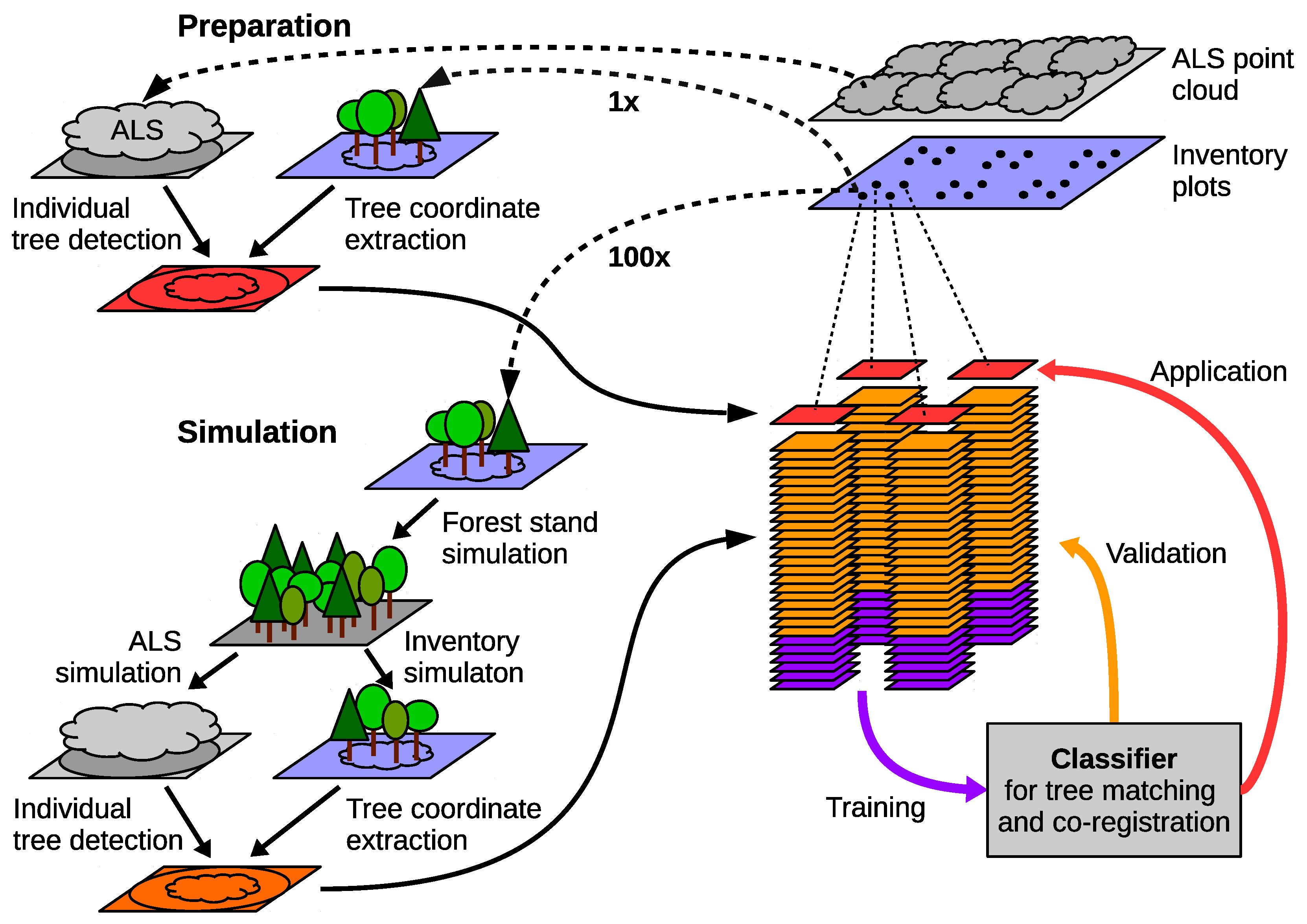
2.1. Inventory Data

To develop and evaluate our co-registration method, we used inventory plots from the latest BWI (2011–2012) within the area of Hunsrück-Hochwald National Park located in Rhineland-Palatinate, Germany (Figure 1). The plot centers are arranged in a regular 2 km × 2 km grid. The plot centers were measured with differential GPS and projected into the ETRS89/UTM coordinate system.

In the BWI, a tree is recorded as a sample tree according to the angle count sampling technique [32]. As the BWI uses an angle count factor of 4, a tree is hence recorded if its distance to the plot center is less than 25 times its DBH. A further selection criterion for a tree to be recorded is a DBH of at least 7 cm. For each sampled tree, its species and DBH are recorded, whereas the tree height is measured only for a subset of the sample. The remaining tree heights are estimated using regression models based on the DBHs. Finally stand-specific taper functions [33,34] are applied. The tree location is determined by measuring the distance to the plot center and the corresponding azimuth angle.

As a result of this sampling technique, each plot is characterized by an individual maximum radius (determined by the most distant tree) as well as the maximum limiting circle (maximum distance where the strongest tree would still have been selected). The angle count sampling technique realizes the sample inclusion probability of a tree being proportional to its diameter. Therefore, this technique prefers in particular the selection of diameter strong (usually tall) trees.

We focused on plots with at least two recorded trees of at least 4 m height, which resulted in 133 plots (65 plots surveyed 2011 and 76 surveyed 2012). These plots comprise 1015 trees in total, consisting of 43.3% Norway spruce (Picea abies), 37.6% European beech (Fagus silvatica), 4.8% sessile oak (Quercus petraea), 4.4% Douglas fir (Pseudotsuga menziesii), 4.1% European larch (Larix decidua), 3.3% European white birch (Betula pendula), and 2.4% others. Detailed information on the investigated plots is summarized in

Table 1. Basic statistics of the 133 investigated BWI plots. DBH: diameter at breast height; HDOP: horizontal dilution of precision.

Attribute	Minimum	1th Quartile	Median	Mean	3th Quartile	Maximum
DBH (cm)	7.0	23.8	36.2	36.73	47.9	112.5
Tree height (m)	5.2	19.8	24.8	24.65	29.9	50.6
Stems per hectare	48	202	412	742.4	839	6014
Number of recorded trees per plot	2	5	7	7.6	10	16
Maximum radius (m)	0.3	3.0	5.25	5.9	8.1	20.8
Limiting circle radius (m)	2.6	8.9	12.6	12.4	15.7	28.1
HDOP	0.8	1.1	1.2	1.32	1.5	3.2

. As an indicator for the GNSS satellite constellation, the horizontal dilution of precision (HDOP, c.f. [36]) is specified.

2.2. ALS Data

The ALS data acquisition was accomplished from 24 March to 7 April 2015 using a Riegl Q560 [37] under leaf off conditions. The mean flying height above ground was 600 m, and resulted in a footprint diameter of about 0.3 m and an average pulse density of 11.2 pulses per m². The ALS datasets were provided by the state forest service of Rhineland-Palatinate in the form of pre-classified (ground vs. other classes) LAS-files. For each of the investigated BWI plots, we selected a circular subset with a radius of 38 m around the plot center.

3. Methods

3.1. Definitions

Each tree t is characterized by its coordinates $t_x$ and $t_y$, as well as its height $t_h$. Thus, a tree can also be seen as a three-dimensional point. For a better mathematical formulation, a set of m trees shall be represented by a matrix of homogeneous coordinates $M^{m\times 4}$, such that a tree is defined by $(t_x,t_y,t_h,1)\in M$. This representation allows a translation of M in direction $\overrightarrow{v}=(v_x,v_y,v_h)$ by applying the matrix multiplication $T_{v}M$, with $T_v$ defined by Equation (1).

$$T_v=\left[\begin{array}{cccc}1& 0& 0& v_x\\ 0& 1& 0& v_y\\ 0& 0& 1& v_h\\ 0& 0& 0& 1\end{array}\right]$$

(1)

Following these definitions, each survey plot forms a data-set with a set of surveyed trees S and a set of detected trees D. A potential tree pair $(s,d)$ with $s\in S$ and $d\in D$ is named Matching if s actually corresponds to d, but Not matching otherwise. Consistently, a set of potential tree pairs is assumed to be correct if at least 50% of the tree pairs are classified as Matching. The probability of a correct co-registration (GNSS error successfully identified using matching tree pairs) will be called “co-registration probability”.

3.2. Digital Terrain Model (DTM) Generation

A digital terrain model (DTM) is generated for each plot based on filtered ALS points. To achieve these filtered points all points already classified as ground are selected. Then each ground point is investigated iteratively in ascending order of z-coordinate. For a given point, all points within a horizontal radius of 0.8 m are removed, except for the one with minimum z-coordinate. This procedure results in a subset of ground points which is characterized by a point spacing of 0.8 to 1.6 m. A Delaunay triangulation of this subset finally serves as DTM.

3.3. Individual Tree Detection

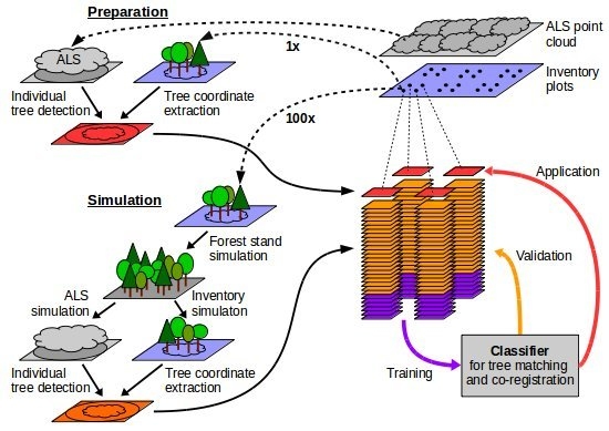
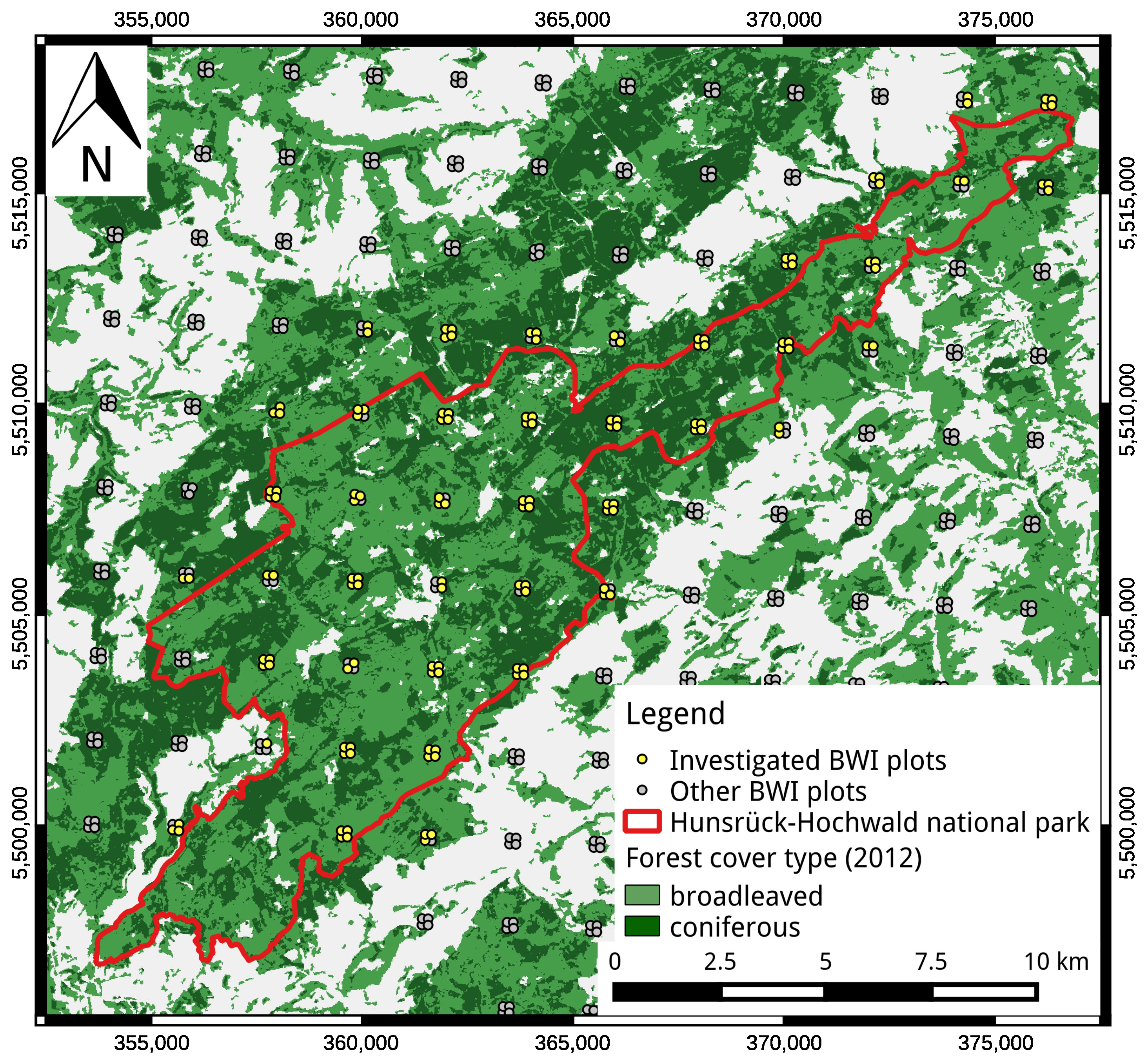
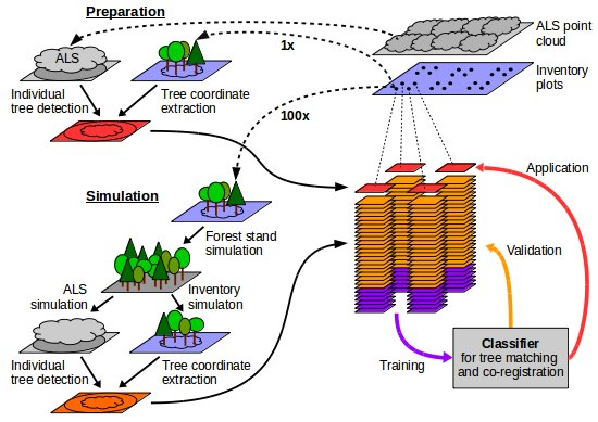
Since the angle counting technique prefers the selection of diameter strong (usually tall) trees, the detection of particularly dominant trees is expedient to register surveyed trees and detected trees. In the context of matching these surveyed trees to ALS detected trees, an identification of small or suppressed trees is not necessary. Thus, we decided to detect individual trees by identifying local maxima within the ALS point clouds. Hence, a point is assumed to correspond to the top of a tree if no point within a radius of 3 m has greater z-values. The threshold of 3 m seemed to be feasible due to the observed stand densities and the ALS pulse density. Unreliable tree detections might reduce the performance of the proposed algorithm, but may help to develop a robust approach. The heights of the detected trees are estimated by height normalization using the DTMs. To avoid commission errors, detections with heights below 4 m and with a horizontal distance to the plot center above 33 m are omitted.

3.4. Simulation

Usually, the exact spatial location of a survey plot center is unknown; studies focusing on co-registration [4,17] identify the most probable location by visually interpreting CHMs or aerial images. An objective expert judgment can be severely affected by the individual experience of the interpreter, data-quality, and forest characteristics. Since automated co-registration methods optimize the accordance between the surveyed data (e.g., tree heights) and remote sensing data (e.g., CHM), an operator will unintentionally tend to the solution proposed by the algorithm. Thus, a posteriori validation might lead to a bias towards the proposed solution [17], which leads to an overestimation of the algorithm performance. If ambiguous sample plots are excluded from validation (as in [4,17]), a further source of overestimation is introduced, since the algorithm is only assessed for simple cases. Even if the correct plot location has been unambiguously identified, a comparison to a location identified by an algorithm is problematic because of remaining positional errors.

Olofsson et al. [20] already introduced an alternative and more promising approach for validating the co-registration and tree matching results by simulating forest stands. Since the corresponding tree pairs are known, the correctness of the results can be tested unambiguously. Based on the need for synthetic training and validation data, the study design illustrated in Figure 2 has been elaborated.

3.4.1. Forest Stand Simulation

For each of the BWI sample plots within our study area, we simulated one hundred synthetic forest stands with a circular area of 0.7 ha using the Waldplaner 2.0 [38] software. The Waldplaner software generates simulated forest stands based on forest inventory data using the single-tree-based forest growth model treeGROSS [39]. Based on the inventory data from a sample plot, treeGROSS estimates species-specific stem number and diameter distributions that serve as an initialization of a simulated forest stand. Subsequently, parameters such as DBH, tree height, crown base height, and width are then predicted for each individual tree using allometric functions. Since the small number of trees allows no conclusion about the actual spatial distribution, uniformly-distributed initial tree locations were assumed. The spatial location of each tree was finally modeled by taking crown competitions between the simulated tree individuals into account. For the subsequent accuracy assessment of the proposed approach, each tree was finally labeled with a unique ID.

3.4.2. Synthetic Inventory Data

We derived synthetic inventory data in each simulated stand by applying the BWI sampling technique after randomly relocating (GNSS error) the plot center. Each tree is labeled with the ID taken from the synthetic stand. Based on literature research on GNSS accuracy (Section 1.1) and a preliminary visual appraisal of GNSS errors occurring for the investigated BWI plots, we assumed normally-distributed planar GNSS errors with a standard deviation of 8 m. To reflect the specifications of [40], we simulated inaccuracies of the tree coordinates by adding normally-distributed residuals with a standard deviation of 1.5% of planar distance to the plot center, as well as compass errors with a standard deviation of 0.8°. We simulated height measurement errors by adding residuals with a standard deviation of 4% of the tree height.

3.4.3. Synthetic Tree Detections

Simulated ALS point clouds were generated to derive synthetic tree detections. Like Frazer et al. [7], we assumed vegetation surfaces impervious to the laser beam, a nadir orientation, and an infinitely small footprint. The point clouds (Figure 3) were created by modeling the light crown of each simulated tree according to relationships published by Pretzsch [41].

A tree crown is defined by the tree species-specific parameters b and c (see

Table 2. Tree species-specific light crown model parameters according to Pretzsch [41]. Values indicated in italics were based on assumption, since they were not given by Pretzsch [41]. Reproduced with permission from Eugen Ulmer Verlag, 2017.

Species	c	b
Quercus petraea (sessile oak)	0.50	0.50
Fagus silvatica (European beech)	0.40	0.33
Abies alba (European fir)	0.50	0.50
Alnus glutinosa (European alder)	0.56	0.50
Picea abies (Norway spruce)	0.66	1.00
Pseudotsuga menziesii (Douglas fir)	0.66	1.00
Pinus silvestris (Scots pine)	0.64	0.50
Larix decidua (European larch)	0.80	0.45

), the tree height h, crown base height $cbh$, and its crown radius r (all provided by the Waldplaner 2.0 software, [38]). The height above ground $e_i$ of a point with distance $d_i$ to the tree location less than or equal to r is calculated by Equation (2). Please note that since the parameters of the Douglas fir were not given by Pretzsch [41], these were assumed to be similar to the parameters of the Norway spruce.

$$e_i=h-c·(h-cbh)·{\left(\frac{d_i}{r}\right)}^{\frac{1}{b}}$$

(2)

For each plot, we generated uniquely-distributed xy-coordinates with the same pulse density as the original point cloud. For each point, the z-coordinate was calculated by applying Equation (2) for all trees and adding the value of the DTM (of the original ALS point cloud) at the tree location. Finally the point is linked to the tree which resulted in the maximum z-coordinate and—for a subsequent evaluation—it is labeled with the ID of that tree.

Since the use of crowns shape functions might result in well-shaped crowns, which would allow an unambiguous co-registration, we simulated irregularities by adding residuals. After a coarse manual optimization (with the aim of realistic tree detection characteristics), we chose normally-distributed horizontal residuals with a standard deviation of 1.5 m and gamma-distributed vertical residuals with a shape of 3 and a scale of 0.3 m.

Finally, the tree detection method presented in Section 3.3 was applied to each synthetic point cloud. To allow an accuracy assessment, each detected tree was labeled with its tree ID taken from the point cloud. If a tree was detected multiple times, only the detection with the tallest z-coordinate was labeled.

3.5. Simulation Quality Assessment

When using simulations for algorithm training and validation, it must be considered that characteristics such as the spatial distribution of the trees can have severe impacts on a successful registration and the transferability of the method. Therefore, a high similarity between the actual and simulated forest stands has to be guaranteed. Assuming full comparability between the synthetic and the original datasets, similar point statistics should be achieved. Consequently, we evaluated the number of trees, the number of detections per reference tree, and the mean nearest-neighbor distance $\overline{NND}$ (Equation (3)) for all training datasets overall and on the plot level.

$$\begin{array}{c}\hfill \begin{array}{cc}\hfill \overline{NN{D}_A}=& \sum _{d\in \underset{a\in A}{NN{D}_a}}\frac{d}{|A|}\hfill \\ \hfill \underset{a\in A}{NN{D}_a}=& \underset{b\in A\setminus \left\{a\right\}}{min}{\parallel b-a\parallel }_2\hfill \end{array}\end{array}$$

(3)

To assess the suitability of the simulated datasets, various statistical analyzes of the previously mentioned variables have been performed. To decide if the values between the original and simulated datasets generally differ, the two sample Wilcoxon rank sum test (comparison of medians) and the F-test (comparison of variances) have been performed. To evaluate the correlation between the original and the simulated values on plot level, the Pearson’s correlation coefficient has been calculated. To investigate the overall agreement on plot level, the RMSE has been calculated and a paired Wilcoxon rank sum test has been applied for each plot. We have chosen the nonparametric Wilcoxon test to not rely on normally distributed data.

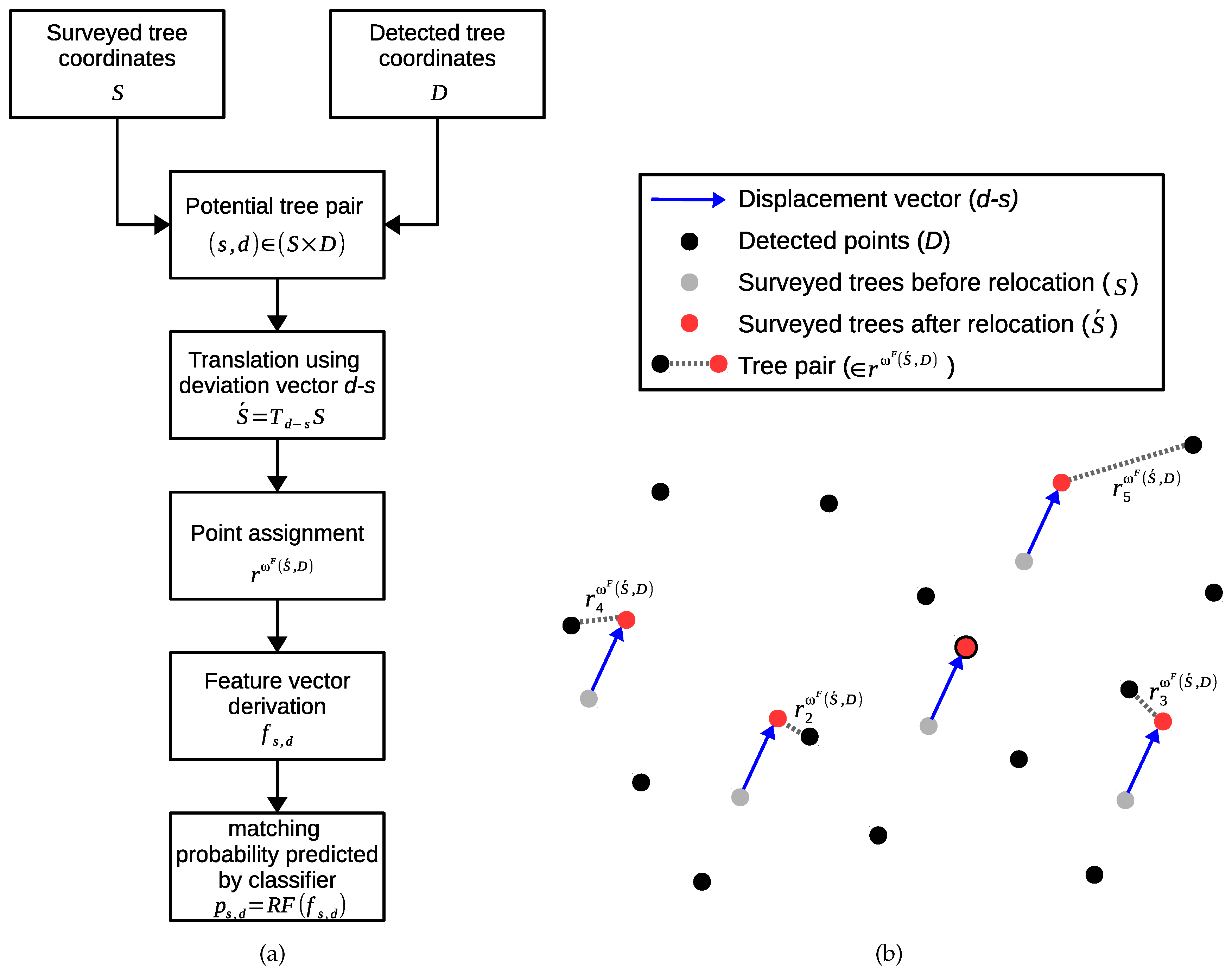
3.6. Classification-Based Tree Matching and Co-Registration

We developed a tree-matching and co-registration method which consists of two major components.

• Classification-based estimation of the matching probability for each potential tree pair.
• Co-registration of the survey trees based on the estimated matching probabilities.

Since both components require linking surveyed trees and detected trees, we firstly define a generic point assignment process. We also define a method for pure distance based tree assignment.

3.6.1. Point Assignment Process

The generally defined point assignment process assigns unique pairs of two n-dimensional point sets A and B. To assign the point pairs hierarchically, we define some kind of weight ${\omega }_{a,b}\in {\mathbb{R}}_{\ge 0}$ for each potential point pair $(a,b)\in (A\times B)$. The point assignment is performed in ascending order of these weights, which results in a finite sequence $r^{\omega (A,B)}$ of $|r^{\omega (A,B)}|$ point tuples (Equation (4)). In particular, we define the subsequence $r_{\le k}^{\omega (A,B)}$ (Equation (5)), which comprises at most k point pairs.

$$\begin{array}{c}{r}^{\omega (A,B)}={\left(r_i^{\omega (A,B)}\right)}_{i\in \{1,\cdots ,|r^{\omega (A,B)}|\}}\\ |r^{\omega (A,B)}|={\displaystyle \sum _{i=1;r_i^{\omega (A,B)}\ne \varnothing }^{min(|A|,|B|)}}1\end{array}$$

(4)

$$r_{\le k}^{\omega (A,B)}={\left(r_i^{\omega (A,B)}\right)}_{i\in \{1,\cdots ,k-1\}}$$

(5)

The elements of $r^{\omega (A,B)}$ are recursively defined by Equation (6). Note that this definition requires all weights greater zero to be strictly ordered. For simplification reasons, only the first element (in order of occurrence) is selected in the case of similar weights. Since each point $a\in A$ can only be assigned to at most one point $b\in B$ and only point pairs with weight greater than zero can get assigned, the magnitude $|r^{\omega (A,B)}|$ is at most the minimum of $|A|$ and $|B|$.

$$\begin{array}{c}\begin{array}{cc}\hfill r_1^{\omega (A,B)}=& \underset{(a,b)\in (A\times B)}{argmax}{\omega }_{a,b}\hfill \\ \hfill r_i^{\omega (A,B)}=& \underset{(a,b)\in (A\times B)\mid \forall (\acute{a},\acute{b})\in r_{\le i-1}^{\omega (A,B)}:a\ne \acute{a}\wedge b\ne \acute{b}}{argmax}{\omega }_{a,b}\hfill \end{array}\\ \underset{(a,b)\in C}{argmax}{\omega }_{a,b}=\{(a,b)\in C\mid {\omega }_{a,b}>0\wedge \forall (\acute{a},\acute{b})\in C:{\omega }_{\acute{a},\acute{b}}\le {\omega }_{a,b}\}\end{array}$$

(6)

3.6.2. Distance-Based Tree Assignment

To assign trees within a given distance and to combine the two-dimensional neighborhood criterion with the height criterion of e.g., [3] we define the $ϵ$-norm ${\parallel ·\parallel }_{ϵ}$ (Equation (7)). The key idea of this $ϵ$-norm is that a surveyed tree $s\in S$ can only be assigned to a detected tree $d\in D$ if ${\parallel d-s\parallel }_{ϵ}\le 1$. From ${\parallel d-s\parallel }_{ϵ}\le 1$ follows ⇒$|d_x-s_x|\le {ϵ}_x$, $|d_y-s_y|\le {ϵ}_y$ and $|d_h-s_h|\le {ϵ}_h$.

$${\parallel v\parallel }_{ϵ}=\sqrt{{\left(\frac{v_x}{{ϵ}_x}\right)}^2+{\left(\frac{v_y}{{ϵ}_y}\right)}^2+{\left(\frac{v_h}{{ϵ}_h}\right)}^2}$$

(7)

Based on this $ϵ$-norm, we define a tree assignment method which returns a sequence of linked trees $r^{{\omega }^{ϵ}(S,D)}$ using the weights ${\omega }^{ϵ}(S,D)$ (Equation (8)) as presented in Section 3.6.1. This corresponds to a tree assignment in ascending order of tree pair distance.

$${\omega }^{ϵ}(A,B)={\left({\omega }_{a,b}^{ϵ}=\left\{\begin{array}{cc}0,\hfill & {\mathrm{if}\parallel b-a\parallel }_{ϵ}>1\hfill \\ \frac{1}{{\parallel b-a\parallel }_{ϵ}},\hfill & \mathrm{if}a\ne b\hfill \\ \infty ,\hfill & \mathrm{otherwise}\hfill \end{array}\right.\right)}_{a\in A;b\in B}$$

(8)

3.6.3. Classification-Based Tree Matching

Following the idea of feature descriptors, the proposed tree matching method derives features which have the potential to classify each potential tree pair $(s,d)\in (S\times D)$ of surveyed trees S and detected trees D as either Matching or Not matching. These features serve as input for a Random Forest [42,43] classifier to estimate the probability $p_{s,d}$ of the class Matching (hereafter “matching probability”).

Caused by GNSS errors, a shift between the surveyed trees S and detected trees D has to be assumed. Thus, the displacement vector between both point sets S and D has to be estimated. Assuming a surveyed tree $s\in S$ corresponds to a detected tree $d\in D$, the displacement vector is approximately $d-s$, and we can perform a GNSS correction by applying $T_{d-s}S$. Since we can assume displacements similar to the GNNS errors, the probability $p_{s,d}$ should decrease with increasing values for $|d_x-s_x|$ and $|d_y-s_y|$.

Further, we assume the surveyed tree s matches the detected tree d, which results in almost similar point patters $T_{d-s}S$ and D. Thus, we can find a set of k neighbored tree pairs $r_{\le k}^{{\omega }^F(T_{d-s}S,D)}$ which is characterized by point pair distances $\parallel r^{{\omega }^F(T_{d-s}S,D)}{\parallel }_2$ (Equation (10)) close to zero. Note that the weights ${\omega }^F(T_{d-s}S,D)$ (Equation (9)) result in a tree pair assignment in ascending order of distance. Missing tree pairs (which occur if $k>min(|S|,|D|)$) are indicated with infinite weights. Assuming s does not match d, then we would expect larger point pair distances, because here the point patterns will most likely differ. Thus, the point pair distances $\parallel r^{{\omega }^F(T_{d-s}S,D)}{\parallel }_2$ serve as a sequence of features to indicate similar point patterns.

$${\omega }^F(A,B)={\left({\omega }_{a,b}^F=\left\{\begin{array}{cc}\frac{1}{{\parallel b-a\parallel }_2},\hfill & \mathrm{if}a\ne b\hfill \\ \infty ,\hfill & \mathrm{otherwise}\hfill \end{array}\right.\right)}_{a\in A;b\in B}$$

(9)

$$\begin{array}{c}\parallel r^{\omega (A,B)}{\parallel }_2={\left(\parallel r_i^{\omega (A,B)}{\parallel }_2\right)}_{i\in \{1,\cdots ,|r^{\omega (A,B)}|\}}\\ \parallel r_i^{\omega (A,B)}{\parallel }_2=\left\{\begin{array}{cc}\infty ,\hfill & \mathrm{if}{r}_i^{\omega (A,B)}=\varnothing \hfill \\ {\parallel b-a\parallel }_2\mathrm{with}(a,b)=r_i^{\omega (A,B)},\hfill & \mathrm{otherwise}\hfill \end{array}\right.\end{array}$$

(10)

For a given sequence of matching tree pairs r, an almost one-to-one correlation between the tree heights $h_S\left(r\right)$ and $h_D\left(r\right)$ (Equation (11)) should be observable. Mismatched trees should lead to uncorrelated tree heights. Thus, the Pearson’s correlation coefficient $\rho$ of these heights serves as an additional feature of the pair $(s,d)$.

$$\begin{array}{cc}\hfill h_S\left(r\right)=& {\left(s_h\right)}_{(s,d)\in r}\hfill \\ \hfill h_D\left(r\right)=& {\left(d_h\right)}_{(s,d)\in r}\hfill \end{array}$$

(11)

In addition to these indicators for similar point patterns, additional features are derived which give information about uncertainties associated with a potential tree pair. Since the probability of identifying a correct tree pair by chance decreases with an increasing number of potential tree pair combinations, the number of trees $|S|$ and $|D|$ serve as additional features. Since close-standing trees complicate the unambiguous identification of matching tree pairs, the average nearest-neighbor distances $\overline{NN{D}_S}$ and $\overline{NN{D}_D}$ (Equation (3)) are calculated as an indicator of tree separability.

Based on the given features, a feature vector $f_{s,d}$ (Equation (12)) is calculated for each potential tree pair $(s,d)\in (S\times D)$. Figure 4 visualizes the workflow for deriving such a feature vector. It also illustrates how the set S is relocated by applying the translation matrix $T_{d-s}$ to assign the neighboring tree pairs $R^{{\omega }^F}(T_{d-s}S,D)$.

$$\underset{s\in S;d\in D}{f_{s,d}}=\left(\begin{array}{c}{\parallel d-s\parallel }_2\\ d_x-s_x\\ d_y-s_y\\ d_h-s_h\\ \parallel r_2^{{\omega }^F(T_{d-s}S,D)}{\parallel }_2\\ ⋮\\ \parallel r_k^{{\omega }^F(T_{d-s}S,D)}{\parallel }_2\\ |S|\\ |D|\\ \overline{NN{D}_S}\\ \overline{NN{D}_D}\\ {\rho }_{h_S\left(r_{\le k}^{{\omega }^F(T_{d-s}S,D)}\right),h_D\left(r_{\le k}^{{\omega }^F(T_{d-s}S,D)}\right)}\end{array}\right)$$

(12)

The classifier needs to be trained using a series of representative datasets with known matching tree pairs. For each dataset (with S and D) and each potential tree pair $(s,d)\in (S\times D)$, the feature vector $f_{s,d}$. The class information is taken from the tree ID labels mentioned in Section 3.4.2 and Section 3.4.3. Thus, a tree pair is classified as Matching if the ID of s corresponds to the ID of d, and as Not matching otherwise. Finally, all of these feature vectors and class information are used to train the random forest classifier $RF$. After this step, it is able to predict the matching probability $p_{s,d}$ (Equation (13)) for each potential tree pair $(s,d)\in (S\times D)$ for two tree sets of surveyed trees S and detected trees D. Finally the tree pair $(s,d)$ is classified as Matching, if the matching probability exceeds 0.5, but Not Matching otherwise.

$$\underset{s\in S;d\in D}{p_{s,d}}=RF\left(f_{s,d}\right)$$

(13)

3.6.4. Co-Registration Method

Since the tree matching method presented in Section 3.6.4 only gives information about the estimated matching probability for single tree pairs, a further method is required which finally identifies the most probable set of tree pairs $r_{after}$.

The proposed co-registration algorithm initially selects all candidate pairs $(s,d)\in (S\times D)$ with a matching probability $p_{s,d}$ (Section 3.6.3) greater than zero. For each of these candidate pairs, the tree set S is shifted by the preliminary displacement vector $d-s$ to derive the tree pair sequence $r^{{\omega }^C(T_{d-s}S,D)}$. The weights ${\omega }^C(T_{d-s}S,D)$ (Equation (14)) correspond to a distance-based tree assignment (Section 3.6.2) in ascending order of matching probability.

$${\omega }^C(A,B)={\left({\omega }_{a,b}^C=\left\{\begin{array}{cc}0,\hfill & {\mathrm{if}\parallel b-a\parallel }_{ϵ}>1\hfill \\ p_{a,b},\hfill & \mathrm{otherwise}\hfill \end{array}\right.\right)}_{a\in A;b\in B}$$

(14)

As such a tree pair sequence might include pairs with low probabilities, the pair with lowest probability is omitted iteratively until the probability $p^{correct}\left(r\right)$ (Equation (15)) of this subsequence r exceeds 0.5. If this threshold is not exceeded, the subsequence with highest probability is kept.

$$\begin{array}{c}{p}^{correct}\left(r\right)=p_{\ge 50\%}^{total}\left(\{p_{a,b}\mid (a,b)\in r\}\right)\\ p_{\ge 50\%}^{total}\left(P\right)={\displaystyle \sum _{\begin{array}{c}\widehat{P}\subset P\\ 2·|\widehat{P}|\ge |P|\end{array}}}{\displaystyle \prod _{p\in \widehat{P}}}p{\displaystyle \prod _{q\in \widehat{P}\setminus Q}}(1-q)\end{array}$$

(15)

Finally, the point pair sequence or subsequence $r_{after}(S,D)$ with highest achieved co-registration probability $p^{correct}\left(r_{after}(S,D)\right)$ is returned by the algorithm. The result is classified as Co-Registration successful, if the co-registration probability exceeds 0.5, but Co-Registration failed otherwise. The final displacement vector ${\overrightarrow{t}}_{after}(S,D)$ (Equation (16)) is calculated by coordinate weighting, which results in a predicted GNSS error of $|{\overrightarrow{t}}_{after}(S,D)|$ m.

$${\overrightarrow{t}}_{after}(S,D)=\sum _{(s,d)\in r_{after}(S,D)}{p}_{s,d}·(d-s)$$

(16)

3.7. Application

We implemented the co-registration and point matching method using python 2.7.6 and standard parametrization of the scikit-learn random forest implementation [44,45] with 50 decision trees, which enables a resolution of the predicted probabilities of 2%; 25% and 75% of the simulated datasets served for algorithm training and for accuracy assessment, respectively.

As more tree pairs do not necessarily lead to better results, we set the parameter k to 15. The suitability of this parameter has been subsequently confirmed, since not more than 14 tree pairs have been assigned. To define the $ϵ$-norm (Equation (7)), the distances between the synthetic inventory trees and their corresponding detections were analyzed. Based on these results and values reported in literature (Section 1.2.2), we set ${ϵ}_x$ and ${ϵ}_y$ to 3.0 m and ${ϵ}_h$ to 4.5 m. These parameters ensure that more than 99% of the these pairs are characterized by an $ϵ$-norm lower than one.

For each of these datasets (with inventory trees S and detected trees D), the co-registration method presented in Section 3.6.4 has been applied. To rate the improvement by relocating the plot centers compared to a naive tree assignment (without considering GNSS errors), we additionally applied the pure distance-based tree assignment method (as presented in Section 3.6.2) using the same $ϵ$-norm. This results in the sequence of potential tree pairs $r_{before}(S,D)$ (Equation (17)) and the probability for at least 50% matching tree pairs $p^{correct}\left(r_{before}(S,D)\right)$. If this probability exceeds 0.5, the sequence $r_{before}(S,D)$ is classified as correct.

$$r_{before}(S,D)=r^{{\omega }^{ϵ}(S,D)}$$

(17)

Finally, we also applied both approaches (with and without GNSS correction) to the original BWI datasets.

3.8. Methods for Accuracy Assessment

To assess the accuracy of the proposed algorithm, confusion matrices were derived using the synthetic validation datasets. Each tree pair $(s,d)$ (assigned by the algorithm) was classified as either Matching or Not Matching (predicted class). The actual class was set to Matching, if s actually corresponds to d, but Not Matching otherwise. A co-registration result was classified by the algorithm as either Co-Registration successful or Co-Registration failed (predicted class). The actual class was set to Co-Registration successful, if at least 50% of the tree assigned tree pairs actually match, and Co-Registration failed otherwise.

If the probabilities predicted by the algorithm (Section 3.6.3 and Section 3.6.4) are in-fact probabilities, we would expect a one-to-one correlation to observed probabilities. To test this, the predicted probabilities for tree matching and co-registration were derived by applying the algorithm using all synthetic validation datasets. Then, equidistant intervals were defined to calculate the average predicted probability and the average observed probability (correct classifications per number of classifications) within each interval. Finally, a regression line was fitted for both tree matching and co-registration.

3.9. Methods for the Evaluation of Feature Importance and Effects

To verify the expectations towards the features, we have analyzed the co-registration results of one randomly selected simulation round. To analyze the effect of a specific feature on the matching probabilities, we have subdivided the results of all plots into three groups. The groups have been defined by the intervals 0–0.33 (low probability), 0.33–0.67 (intermediate probability) and 0.67–1 (high probability). Based on these groups a boxplot has been generated for each feature, which allows conclusions about which values are associated with higher or lower matching probabilities.

To investigate the effect of different forest characteristics on the co-registration performance, we have evaluated the results of all validation datasets. The effect of a selected variable (e.g., tree species) on the co-registration probability has been assessed by grouping the results using equidistant intervals of the variable. Based on these groups a boxplot of the selected variable has been created and a statistical analysis has been performed to support the conclusions. To decide if the values of a given variable differ between the groups (meaning at least one group differs significantly from another group), we have applied the Kruskal–Wallis rank sum test. In case of just two groups the Wilcoxon rank sum test has been used instead, which also gives information about the direction of the effect. In case of ordered groups, we have also verified the significance of potential (linear) trends by performing an one-way ANOVA.

4. Results and Discussion

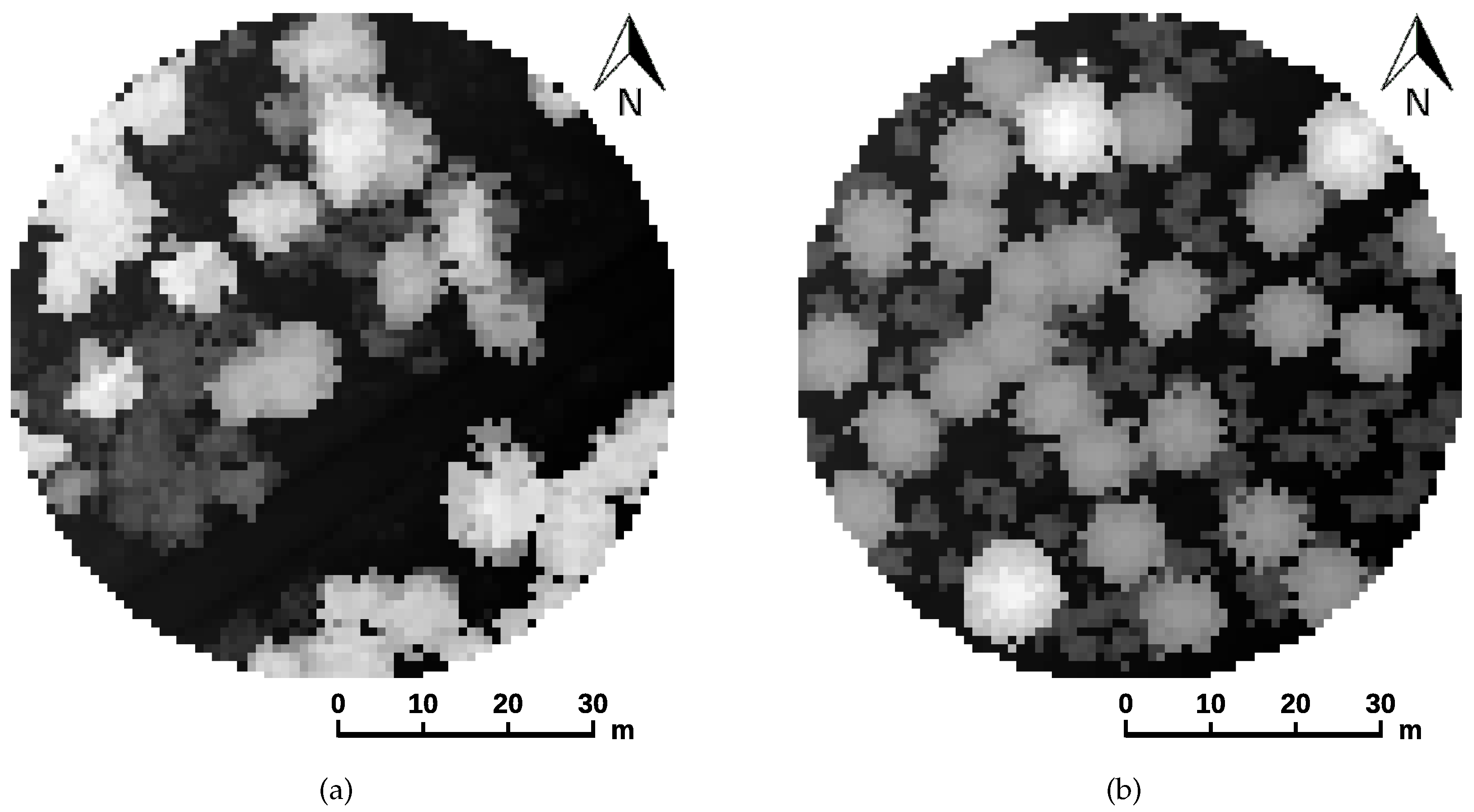
4.1. Quality of the Synthetic Datasets

Using the synthetic forest stand data, the individual tree detection method achieved an average commission error (number of unassigned detections per number of detections) of 11% and an average omission error (number of missed trees per number of reference trees) of 72%. The planar RMSE of the tree positions was about 0.75 ± 0.39 m, and the RMSE of the heights was about 1.21 ± 0.55 m. These accuracy descriptors are consistent with most of the methods benchmarked in [3,11], which indicates an appropriate modeling of the synthetic point clouds. The increased omission rate might be caused by the simplistic detection method and the bias to dominant trees.

Table 3. Evaluation results of the synthetic training data S compared to the original data O. NND: nearest-neighbor distance.

Attribute	Overall			On Plot Level
	Characteristic Values (Minimum, Mean, Maximum)	Two Sample Wilcoxon Test	F-Test	Pearson’s Correlation Coefficient	RMSE	Paired Wilcoxon Test
Amount of Surveyed Trees	$0_{min}=2$; $\overline{O}=7.6$; $O_{max}=16$ $S_{min}=2$; $\overline{S}=7.6$; $S_{max}=22$	$\overline{S}=\overline{O}$ (p = 0.66)	${\sigma }_S={\sigma }_O$ (p = 0.47)	0.98	0.69	$\overline{S-O}>0$ (p = 0.00)
Amount of Detected Trees	$0_{min}=13$; $\overline{O}=46.9$; $O_{max}=83$ $S_{min}=9$; $\overline{S}=46.9$; $S_{max}=104$	$\overline{S}=\overline{O}$ (p = 0.50)	${\sigma }_S>{\sigma }_O$ (p = 0.00)	0.64	15.00	$\overline{S-O}=0$ (p = 0.74)
Amount of Detected Trees per Survey Tree	$0_{min}=1.6$; $\overline{O}=7.9$; $O_{max}=32$ $S_{min}=1.1$; $\overline{S}=7.6$; $S_{max}=49.5$	$\overline{S}=\overline{O}$ (p = 0.69)	${\sigma }_S={\sigma }_O$ (p = 0.91)	0.83	3.30	$\overline{S-O}=0$ (p = 0.33)
Mean NND for Surveyed Trees (m)	$0_{min}=0.5$; $\overline{O}=4.2$; $O_{max}=13.8$ $S_{min}=1.1$; $\overline{S}=5.6$; $S_{max}=27.2$	$\overline{S}>\overline{O}$ (p = 0.00)	${\sigma }_S>{\sigma }_O$ (p = 0.01)	0.81	1.90	$\overline{S-O}<0$ (p = 0.00)
Mean NND for Detected Trees (m)	$0_{min}=4.1$; $\overline{O}=5.4$; $O_{max}=8.2$ $S_{min}=3.7$; $\overline{S}=6.3$; $S_{max}=13.0$	$\overline{S}>\overline{O}$ (p = 0.00)	${\sigma }_S>{\sigma }_O$ (p = 0.00)	0.58	1.36	$\overline{S-O}<0$ (p = 0.00)

summarizes the results of the statistical evaluation of the synthetic training data compared to the original data (overall and on plot level).

The test results for the amount of trees and the amount of detections per reference tree indicate realistic stand densities. The increased average NNDs of the synthetic datasets indicate an overestimation of the tree distances. This effect might be caused by the fact that the original stands are more clustered (e.g., because of aisles or leaning trees), while the simulated trees are distributed more uniformly (with consideration of tree competition). This effect also leads to an incomplete coverage of the value range for this attribute.

As lower NNDs reduce the separability of points, the synthetic inventory plots might be easier to co-register than the original ones. Nevertheless, since the variance within the synthetic datasets is greater than within the original datasets and the value ranges of the other attributes are completely covered, the simulated datasets can be assumed to be appropriate. Thus, by training the algorithm with the synthetic datasets, it should be applicable to the original datasets without losing accuracy.

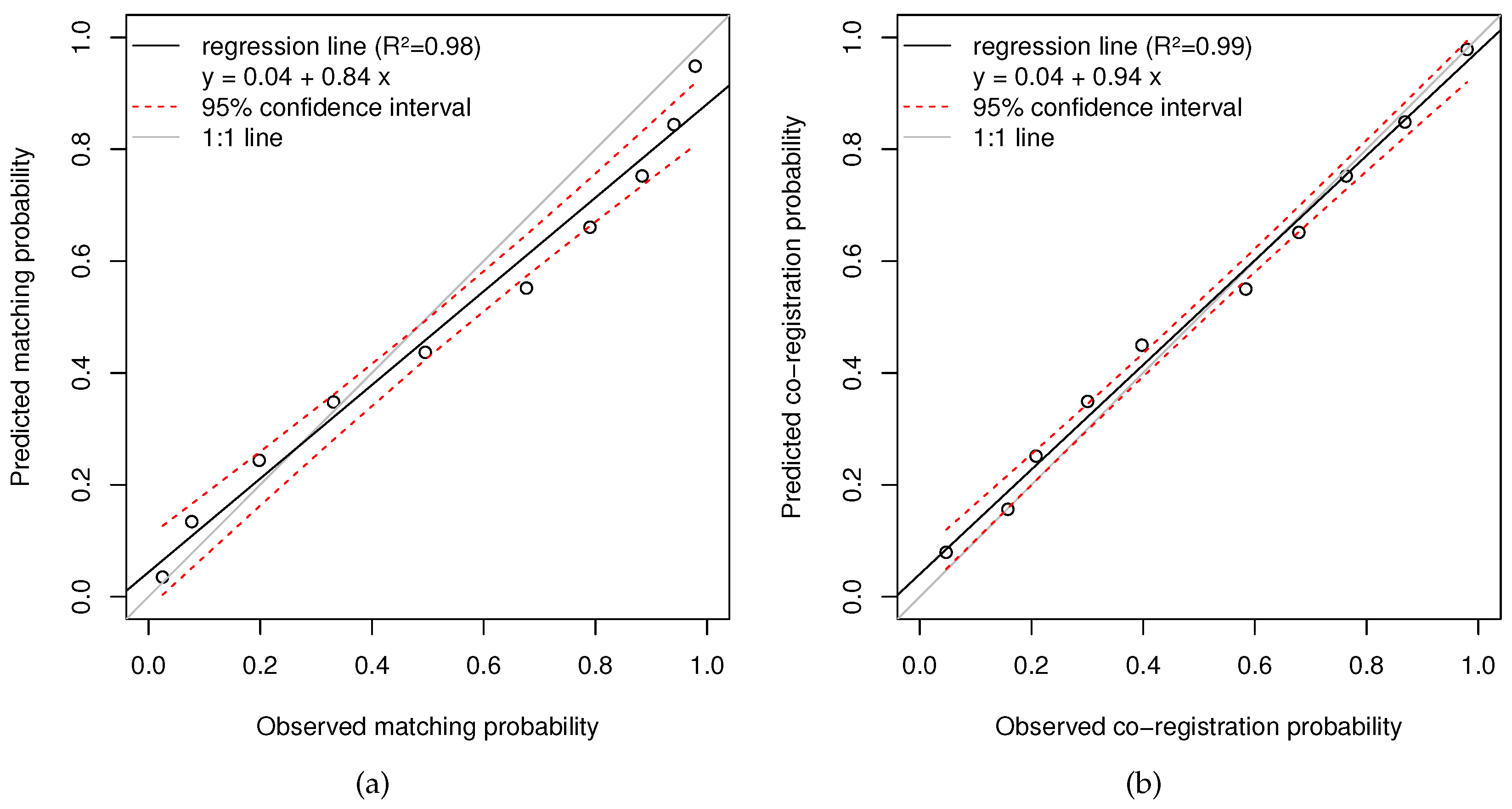
4.2. Accuracy Assessment

The algorithm for individual tree matching (Section 3.6.3) achieved an overall accuracy of 89.1% and a Cohen’s kappa of 0.78 using the synthetic validation datasets (

Table 4. Confusion matrix for tree matching using synthetic validation data.

		Actual Class		Totals	Users’s Accuracy
		Not Matching	Matching
Predicted Class	Not Matching	12,747	1663	14,410	88.5%
	Matching	683	7662	8345	91.8%
Totals		13,430	9325	22,755
Producer’s accuracy		94.9%	82.2%

). The number of matching trees tended to be slightly underestimated, which resulted in a reduced producer’s accuracy.

The proposed co-registration method achieved an overall accuracy of 82.7% and a Cohen’s kappa of 0.70 using the synthetic validation datasets (

Table 5. Confusion matrix for co-registration using synthetic validation data.

		Actual Class		Totals	Users’s Accuracy
		Co-Registration Failed	Co-Registration Successful
Predicted Class	Co-Registration failed	1731	595	2326	74.4%
	Co-Registration successful	890	5377	6267	85.8%
Totals		2621	5972	8593
Producer’s accuracy		66.0%	90.0%

).

Figure 5 illustrates the correlation between the predicted probabilities and observed probabilities (correct classifications per number of classifications) within equidistant intervals for tree matching (Figure 5a) and co-registration (Figure 5b), respectively.

For tree matching, the observed probability was underestimated for values above 0.5, which resulted in a conservative assignment of tree pairs. This effect might be caused by involving the characteristics of almost all trees in the decision process. Since the expected one-to-one relationship was not archived, the predicted probabilities might be handled with caution. To derive real probabilities, a correction of the predicted values (e.g., by using the given regression model) would be necessary.

Although the predicted co-registration probability depends on the predicted matching probability, an almost one-to-one relationship was achieved. These results indicate that the algorithm is able to correctly estimate the reliability of a specific co-registration result.

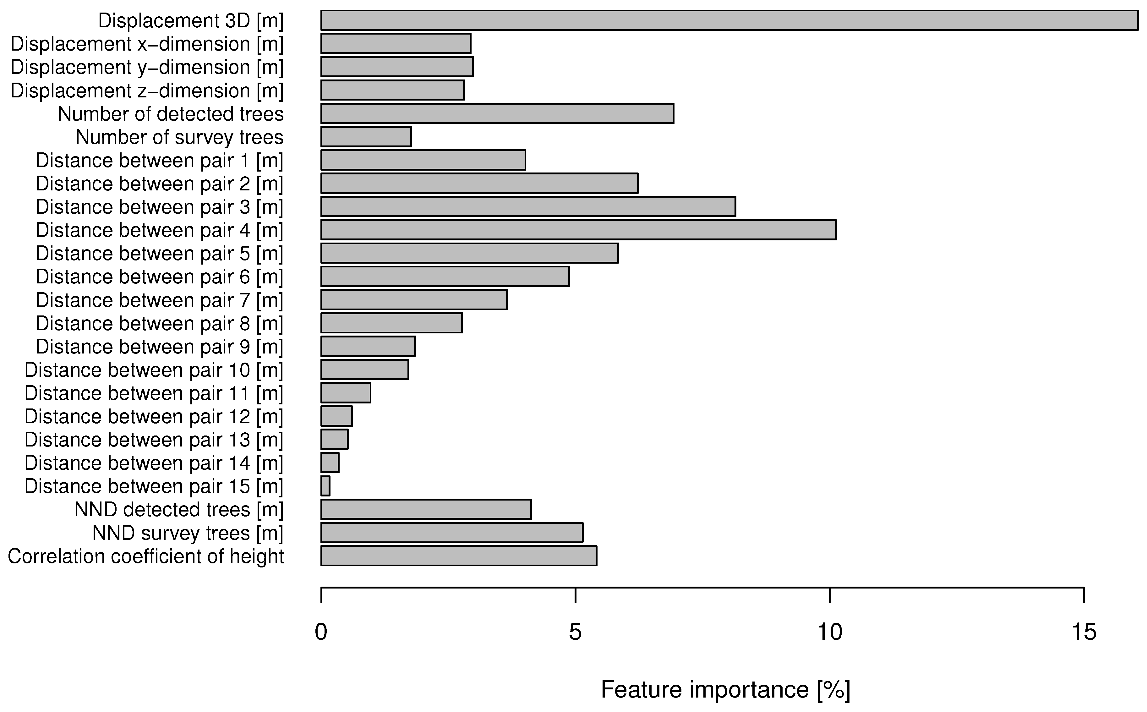
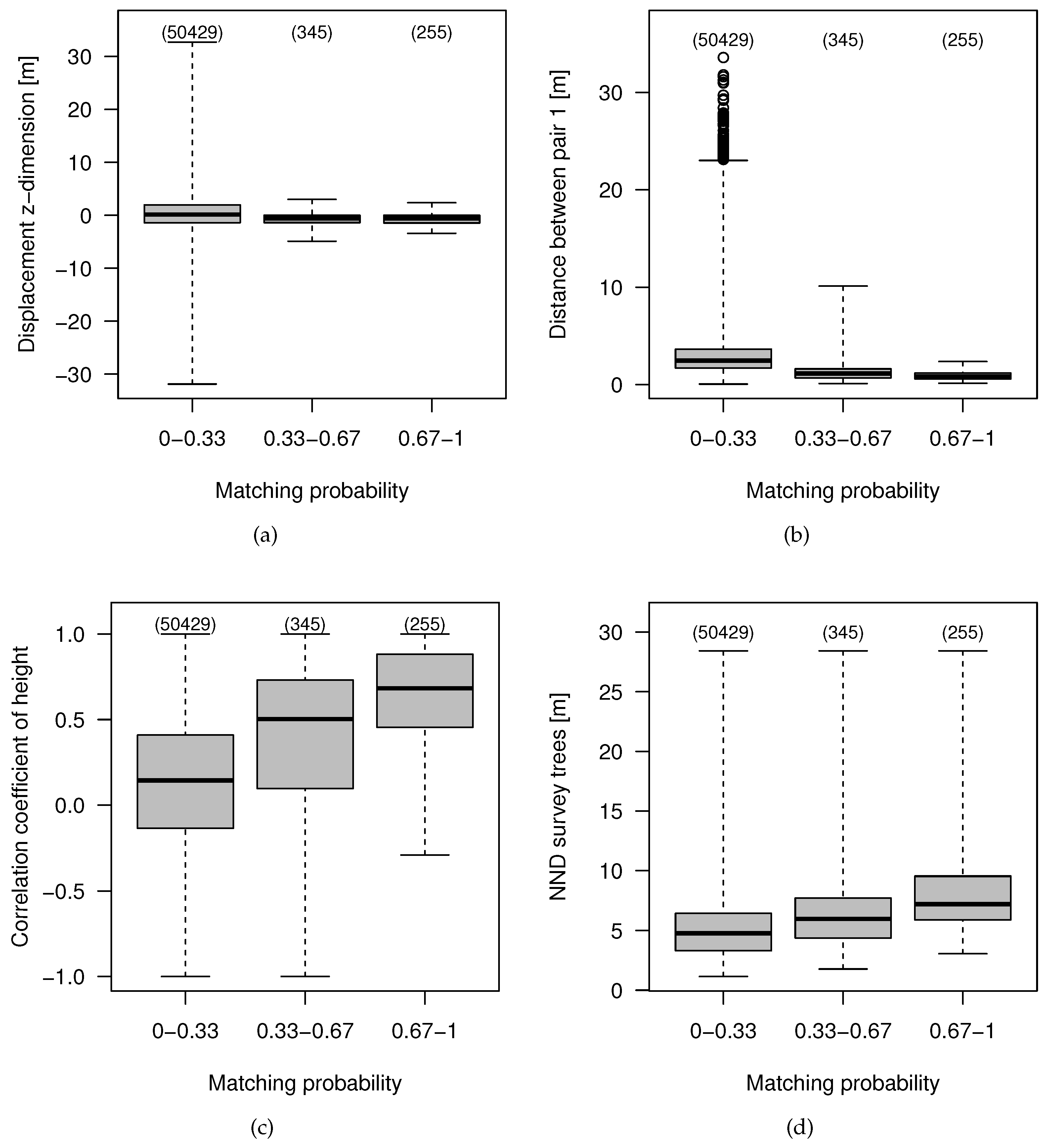
4.3. Feature Importance and Effects

To analyze the meaningfulness of rules identified by the classifier, we accomplished an evaluation of the feature importance and the effects of the features on the matching probability. In general, the rules identified by the classifier aligned with our previous expectations presented in Section 3.6.3. The results of all features can be found in the supplement of the article.

The high feature importance of the 3D displacement and the vertical displacement go along with our prior expectations. Figure 6a illustrates that the highest probabilities were achieved for vertical displacements below 5 m.

Since the distances between the closest tree pairs indicate the agreement of the point patterns, these form the most important group of features. Figure 6b shows that, as expected, low distances to neighbored trees result in high matching probabilities. The ascending importance from the first pair to the fourth pair and the descending importance from the fourth to the fifteenth pair (Figure 7) can be explained by the influence of the number of linked trees. The co-registration probability increases with an increasing number of linked trees, because the certainty that the point patterns match increases with an increasing number of (probably correct) linked trees.

The highest matching probabilities are achieved if a positive correlation between the survey tree heights and ALS tree heights occurs (Figure 6c), which goes along with our previous expectations and the heuristic used by Monnet and Mermin [17], Dorigo et al. [4] or Olofsson et al. [20]. Since the NND is an indicator of the tree separability, the matching probability slightly increases with increasing NNDs (Figure 6d).

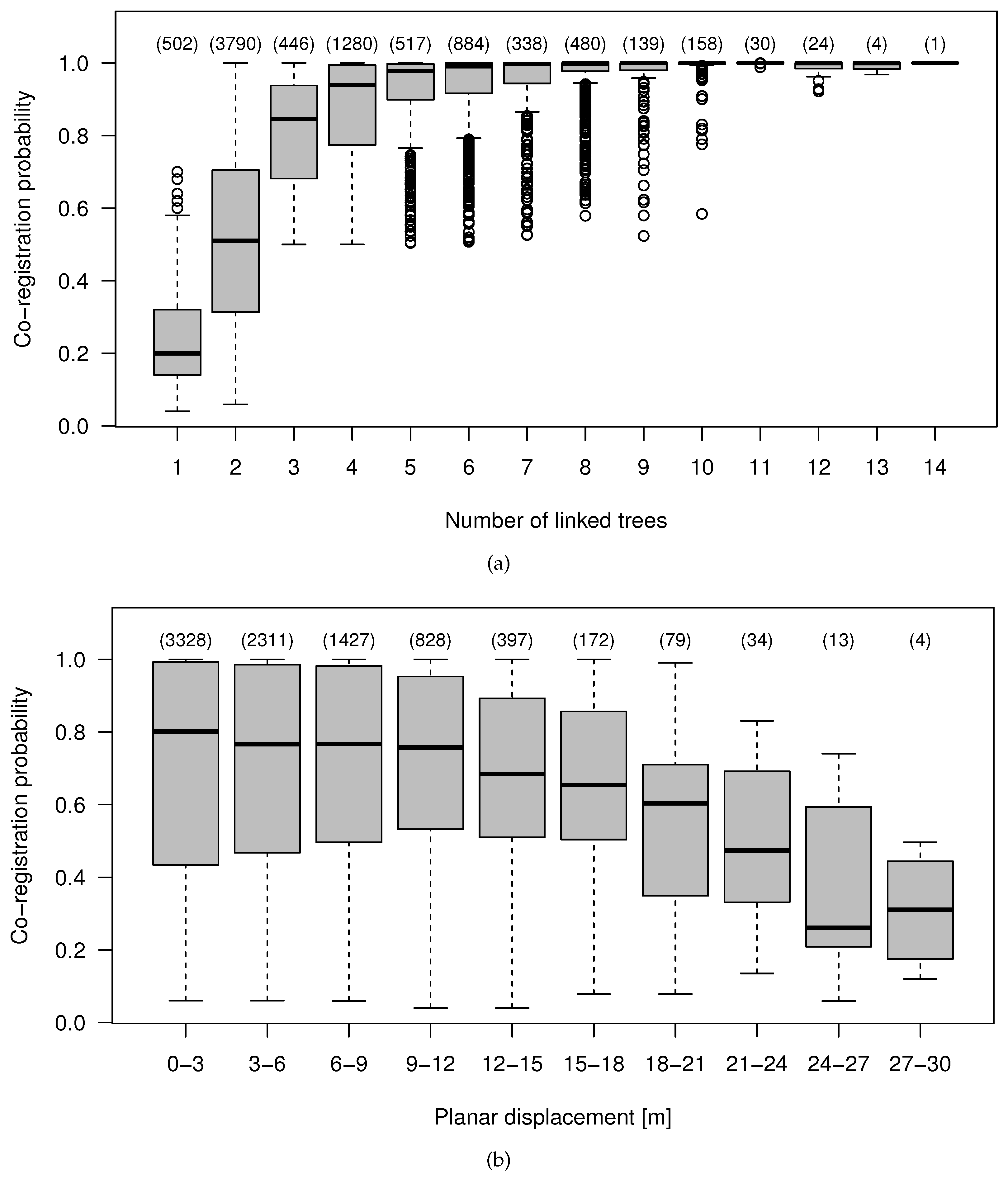
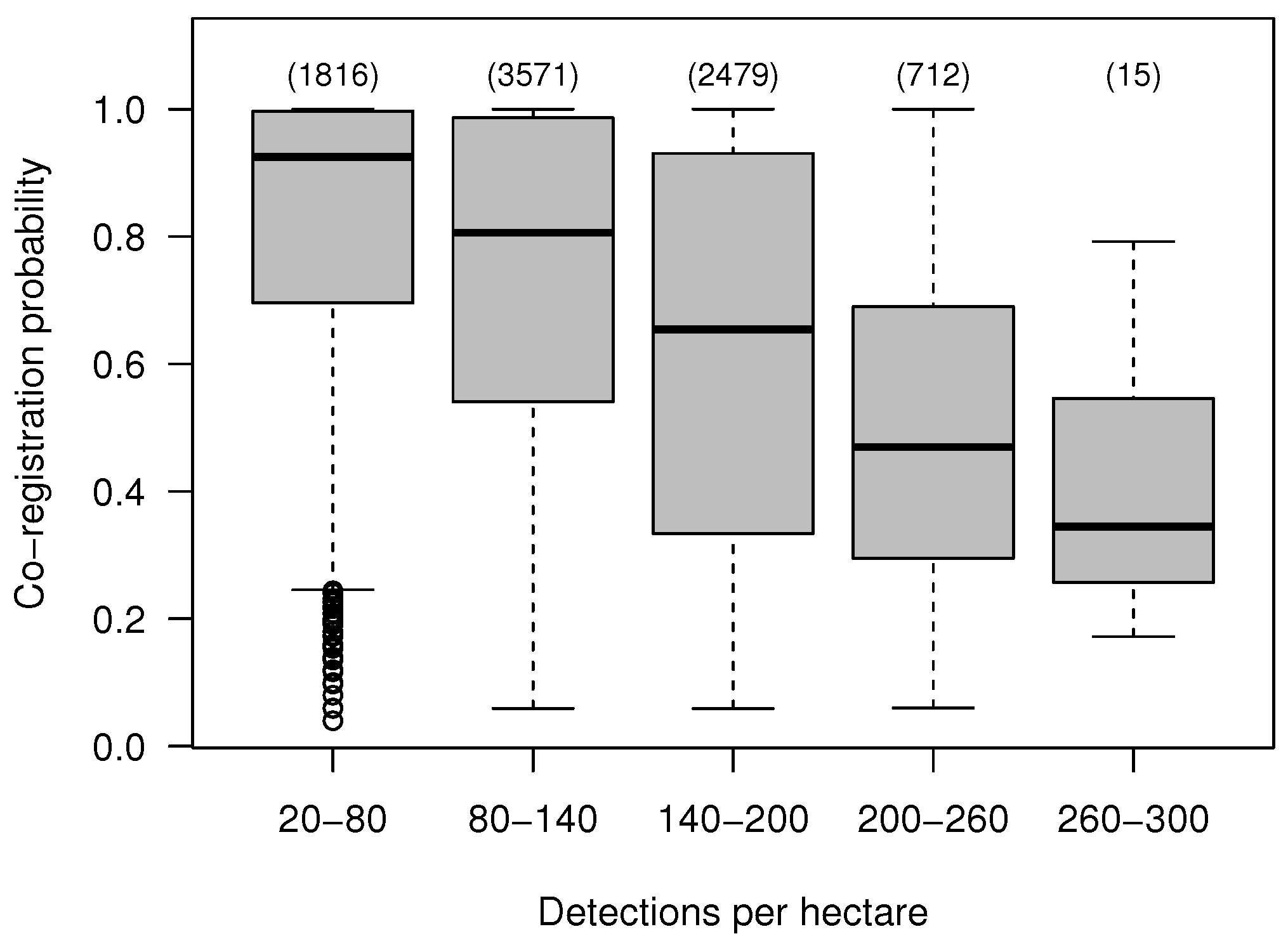
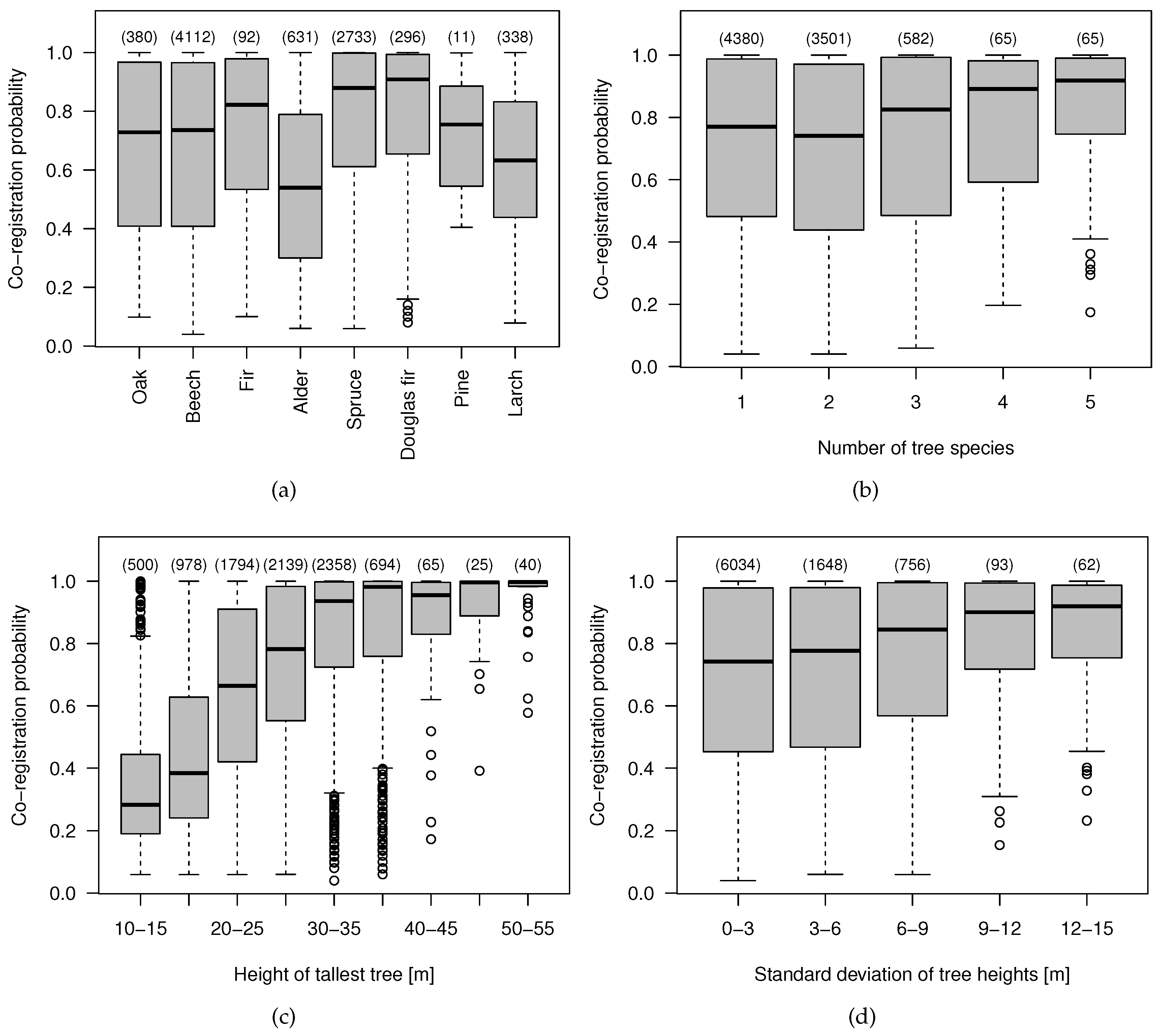
4.4. Effect of the Data Characteristics on the Co-Registration Results

Since the number of linked trees is an indicator of matching point patterns, the probability of a successful co-registration increased with an increasing number of linked trees (Figure 8a). A saturation effect occurred for five links and more (average co-registration probability above 90%), since not every tree pair has to be investigated to decide if the tree patterns match. As desired (by choosing the given GNSS error distribution), the co-registration probability decreased with increasing horizontal displacements (Figure 8b).

Figure 9 illustrates the effect of different forest types and stand characteristics on the co-registration probability. The Kruskal–Wallis rank sum test indicates significant differences of the probabilities between different tree species (p = 0.00). The two-tailed Wilcoxon rank-sum test showed that coniferous trees reached significantly higher probabilities than deciduous trees (p = 0.00), which confirms the findings of previous studies [4,17]. Nevertheless, within the conifers, the larches reach lower probabilities than the other conifers. This effect can be explained by the different crown shapes. Cone-shaped crowns result in higher individual tree detection accuracies and higher location accuracies, which eases the co-registration compared to dome-shaped crowns.

An increasing number of tree species (as an indicator of stand variability) results in a positive effect on the co-registration result. The ANOVA of the co-registration probability grouped by the number of species within a plot (Figure 9b) indicates a significant (linear) trend (p = 0.00).

The ANOVA of the co-registration probability grouped by the height of the tallest tree (Figure 9c) also indicates a significant trend (p = 0.00). A saturation effect for tall trees can be observed. Additionally, the standard deviation of tree heights (Figure 9d) shows a significant linear trend (p = 0.00). With an increasing height of the tallest tree and with an increasing variability of the tree heights, the probability of a correct co-registration also increases, since large values of these variables facilitate the identification of matching tree pairs. These results go along with the findings of Monnet and Mermin [17].

4.5. Method Performance

The proposed method was able to successfully co-register about 69.5% of the synthetic inventory plots, while it linked 81.5% of the tree pairs correctly. By applying a pure distance-based tree assignment (ignoring GNSS errors), only 41.0% of the trees were linked correctly, and the criterion of at least 50% matching tree pairs was fulfilled for only 32.5% of the plots.

The original BWI plots showed similar results. By applying the pure distance-based tree assignment, 288 tree pairs were identified, but only 107 (37%) of these pairs were classified as matching. Only 29 of the plots (22%) fulfilled the criterion of at least 50% tree pairs classified as matching. By applying the proposed co-registration algorithm, 517 tree pairs were assigned. Of these tree pairs, 261 (50%) were classified as matching. The algorithm indicated that 80 of the 133 inventory plots (60%) were co-registered correctly, with 414 assigned tree pairs and 230 (72%) pairs classified as matching. Based on these results, the investigated original BWI plots were characterized by horizontal GNSS errors of up to 21 m, while 80% of the horizontal GNSS errors were in a range between 1.4 and 8.7 m.

Figure 10a illustrates the number of correctly co-registered original BWI plots as a function of the applied co-registration probability. Due to the GNSS correction, the number of co-registered plots increased and higher probabilities were achieved.

Figure 10b illustrates the effect of the year of survey on the co-registration probability. A time-lag between the field survey and the ALS flight campaign (three to four years) might have a negative effect on the co-registration results, since trees might have grown, toppled, or been harvested in this period of time. Although the probabilities of 2011 seem to be slightly lower than the probabilities of 2012, the two-tailed Wilcoxon-test has shown no significantly lower values for 2012 (p = 0.13). However, these results indicate that better results could be achievable if the time lag between inventory and ALS data acquisitions is small.

4.6. Limitations

The analysis of the effect of the time-lag between the field survey and the ALS flight campaign indicates that the proposed co-registration method will be challenged if there is major changes between both dates of observation. This is particularly the case if the trees might have grown, toppled, or been harvested within the time lag between field survey and ALS data collection.

Since we needed to model synthetic training data based on various assumptions, the transfer of the probability estimations to the original datasets should be done with caution. The procedure of simulating ALS point clouds using crown shape functions is justified by the observation that the most ambiguous cases for co-registration occur in dense forest stands, where individual trees are hard to detect because of overlapping crowns. Nonetheless, non representative point clouds might affect the tree detection characteristics. Although the suitability of the simulated datasets has been tested, it cannot be ensured that the datasets are representative. This is particularly the case because the synthetic survey plots were characterized by increased NNDs compared to the original BWI data. However, the usage of simulated forest stands leads to more objective validation results compared to reference locations derived by visual interpretation.

Since the number of potential tree pairs and positional inaccuracies complicates the identification of matching tree pairs, the rudimentary tree detection method used in this study might have a negative effect on the algorithm performance. The ANOVA of the co-registration probability grouped by the number of detections per hectare (Figure 11) indicates a significant trend (p = 0.00). Since the probability for a correct co-registration decreases with an increasing number of detections per hectare, commission errors of the detection method should be avoided. Since the angle count sampling technique prefers the selection of dominant trees, and a correct co-registration is possible with just a few trees assigned (Figure 8a), the reliable identification of the dominant trees is more important than the identification of all trees (which might cause increased commission errors).

Another limitation of the method is that no perfect one-to-one correlation between the predicted and observed probabilities could be achieved. Thus, the predicted matching probabilities provided by the algorithm are a higher order reliability estimation but do not necessarily correspond to actual probabilities. However, since the predicted co-registration probabilities rarely differ from the one-to-one correlation, they seem to represent actual probabilities.

The parametrization of the $ϵ$-norm (defined to assign the tree pairs) should be optimized based on the forest stand characteristics. Since it is only used for the co-registration, it can be adapted for each plot individually after training of the classifier. Using such an optimization might lead to better results compared to the fixed parameters chosen in this study.

5. Conclusions

We performed a co-registration of 133 BWI sampling plots to ALS-derived individual tree detections of a study area in Rhineland-Palatinate, Germany as a preparatory step for a forest characterization on the individual tree level. As erroneous tree pair assignments result in a reduction of model quality (e.g., biomass estimation or tree species classification), we searched for a method for co-registration and tree matching which also rates the reliability of a match.

Since existing methods seemed to be unsuitable for this task, we developed a hybrid co-registration and tree matching algorithm. We trained the machine-learning-based method using synthetic individual tree detections and inventory data, whose representativity has been tested empirically.

The method reached an overall accuracy of 89.7% for tree matching and a user’s accuracy for co-registration of 82.7% using simulated datasets. The method has been applied to the study area, and was able to successfully relocate 60% of the BWI plots, which makes these usable for a further analysis on the individual tree level. As machine-learning methods have been proven powerful to identify patterns, a similar performance of the algorithm compared to a human expert can be expected. Since the interpreter might be biased to the proposed solution, a manual post-processing is not expedient.

The derived feature importance depends on forest characteristics and the assumed GNSS error distribution. The feature importance and its effect on the matching probability has shown to be consistent with prior expectations. Thus, the machine-learning approach seems to be an appropriate alternative to heuristic methods, with the additional advantages of an automated parametrization and a robust estimation of the reliability of a single co-registration and tree matching result.

We found that with five or more linked tree pairs, at least 90% of the co-registration results can be expected to be correct. If the number of terrestrial trees is limited, heuristic methods typically cannot comply with this requirement. We found that the highest probabilities for a correct co-registration were achieved in heterogeneous stands (mixed species, differing tree heights, presence of tall trees). Stands dominated by conifers achieved significantly better co-registration results than stands dominated by deciduous trees. These findings support the results of previous studies.

To achieve better results, the local-maxima-based tree detection method used in this study should be replaced by a more advanced method (e.g., by tree stem detection). Since more accurate tree positions result in a better agreement of the point patterns, the pre-trained algorithm can directly be applied to these more reliable positions without losing explanatory power. To transfer the method to forests with different characteristics or a different sampling design, only an adaption of the (simulated) training datasets is required.

The probability estimations provided by the algorithm—as an objective indicator of the reliability of a specific result—lead to a clear added value compared to existing methods. Since it can serve as a weighting-factor for model training, for example, the proposed method is a relevant tool for gaining further knowledge in the field of forest characterization on small scales or even on the individual tree level.

References

1. Cao, L.; Coops, N.C.; Innes, J.L.; Dai, J.; Ruan, H.; She, G. Tree species classification in subtropical forests using small-footprint full-waveform LiDAR data. Int. J. Appl. Earth Obs. Geoinf. 2016, 49, 39–51. [Google Scholar] [CrossRef]
2. Zhen, Z.; Quackenbush, L.J.; Zhang, L. Trends in Automatic Individual Tree Crown Detection and Delineation—Evolution of LiDAR Data. Remote Sens. 2016, 8, 333. [Google Scholar] [CrossRef]
3. Eysn, L.; Hollaus, M.; Lindberg, E.; Berger, F.; Monnet, J.M.; Dalponte, M.; Kobal, M.; Pellegrini, M.; Lingua, E.; Mongus, D.; et al. A Benchmark of Lidar-Based Single Tree Detection Methods Using Heterogeneous Forest Data from the Alpine Space. Forests 2015, 6, 1721–1747. [Google Scholar] [CrossRef]
4. Dorigo, W.; Hollaus, M.; Wagner, W.; Schadauer, K. An application-oriented automated approach for co-registration of forest inventory and airborne laser scanning data. Int. J. Remote Sens. 2010, 31, 1133–1153. [Google Scholar] [CrossRef]
5. Baltsavias, E.P. Airborne laser scanning: Basic relations and formulas. ISPRS J. Photogramm. Remote Sens. 1999, 54, 199–214. [Google Scholar] [CrossRef]
6. Gobakken, T.; Næsset, E. Assessing effects of positioning errors and sample plot size on biophysical stand properties derived from airborne laser scanner data. Can. J. For. Res. 2009, 39, 1036–1052. [Google Scholar] [CrossRef]
7. Frazer, G.; Magnussen, S.; Wulder, M.; Niemann, K. Simulated impact of sample plot size and co-registration error on the accuracy and uncertainty of LiDAR-derived estimates of forest stand biomass. Remote Sens. Environ. 2011, 115, 636–649. [Google Scholar] [CrossRef]
8. Hyyppä, J.; Yu, X.; Hyyppä, H.; Vastaranta, M.; Holopainen, M.; Kukko, A.; Kaartinen, H.; Jaakkola, A.; Vaaja, M.; Koskinen, J.; Alho, P. Advances in Forest Inventory Using Airborne Laser Scanning. Remote Sens. 2012, 4, 1190–1207. [Google Scholar] [CrossRef]
9. Koenig, K.; Höfle, B. Full-Waveform Airborne Laser Scanning in Vegetation Studies—A Review of Point Cloud and Waveform Features for Tree Species Classification. Forests 2016, 7, 198. [Google Scholar] [CrossRef]
10. Vauhkonen, J.; Ene, L.; Gupta, S.; Heinzel, J.; Holmgren, J.; Pitkanen, J.; Solberg, S.; Wang, Y.; Weinacker, H.; Hauglin, K.M.; et al. Comparative testing of single-tree detection algorithms under different types of forest. Forestry 2011, 85, 27–40. [Google Scholar] [CrossRef]
11. Kaartinen, H.; Hyyppä, J.; Yu, X.; Vastaranta, M.; Hyyppä, H.; Kukko, A.; Holopainen, M.; Heipke, C.; Hirschmugl, M.; Morsdorf, F.; et al. An International Comparison of Individual Tree Detection and Extraction Using Airborne Laser Scanning. Remote Sens. 2012, 4, 950–974. [Google Scholar] [CrossRef]
12. Wallace, L.; Lucieer, A.; Watson, C.S. Evaluating tree detection and segmentation routines on very high resolution UAV LiDAR data. IEEE Trans. Geosci. Remote Sens. 2014, 52, 7619–7628. [Google Scholar] [CrossRef]
13. Hoppus, M.; Lister, A. The status of accurately locating forest inventory and analysis plots using the Global Positioning System. In Proceedings of the Seventh Annual Forest Inventory and Analysis Symposium, Portland, ME, USA, 3–6 October 2007. [Google Scholar]
14. Wing, M.G.; Eklund, A.; John, S.; Richard, K. Horizontal measurement performance of five mapping-grade global positioning system receiver configurations in several forested settings. West. J. Appl. For. 2008, 23, 166–171. [Google Scholar]
15. Andersen, H.E.; Clarkin, T.; Winterberger, K.; Strunk, J. An accuracy assessment of positions obtained using survey-and recreational-grade global positioning system receivers across a range of forest conditions within the Tanana Valley of interior Alaska. West. J. Appl. For. 2009, 24, 128–136. [Google Scholar]
16. Valbuena, R.; Mauro, F.; Rodriguez-Solano, R.; Manzanera, J. Accuracy and precision of GPS receivers under forest canopies in a mountainous environment. Span. J. Agric. Res. 2010, 8, 1047–1057. [Google Scholar] [CrossRef]
17. Monnet, J.M.; Mermin, É. Cross-correlation of diameter measures for the co-registration of forest inventory plots with airborne laser scanning data. Forests 2014, 5, 2307–2326. [Google Scholar] [CrossRef]
18. Luoma, V.; Saarinen, N.; Wulder, M.; White, J.; Vastaranta, M.; Holopainen, M.; Hyyppä, J. Assessing Precision in Conventional Field Measurements of Individual Tree Attributes. Forests 2017, 8, 38. [Google Scholar] [CrossRef]
19. Hollaus, M.; Wagner, W.; Maier, B.; Schadauer, K. Airborne laser scanning of forest stem volume in a mountainous environment. Sensors 2007, 7, 1559–1577. [Google Scholar] [CrossRef]
20. Olofsson, K.; Lindberg, E.; Holmgren, J. A method for linking field-surveyed and aerial-detected single trees using cross correlation of position images and the optimization of weighted tree list graphs. In Proceedings of the SilviLaser 2008—8th International Conference on LiDAR Applications in Forest Assessment and Inventory, Edinburgh, UK, 17–19 September 2008. [Google Scholar]
21. Mongus, D.; Žalik, B. An efficient approach to 3D single tree-crown delineation in LiDAR data. ISPRS J. Photogramm. Remote Sens. 2015, 108, 219–233. [Google Scholar] [CrossRef]
22. Fischler, M.A.; Bolles, R.C. Random Sample Consensus: A Paradigm for Model Fitting with Applications to Image Analysis and Automated Cartography. Commun. ACM 1981, 24, 381–395. [Google Scholar] [CrossRef]
23. Sattler, T.; Leibe, B.; Kobbelt, L. Fast image-based localization using direct 2d-to-3d matching. In Proceedings of the 2011 International Conference on Computer Vision, Barcelona, Spain, 6–13 November 2011. [Google Scholar]
24. Bienert, A.; Pech, K.; Maas, H.G. Verfahren zur Registrierung von Laserscannerdaten in Waldbeständen— Methods for registration laser scanner point clouds in forest stands. Schweiz. Z. Forstwes. 2011, 162, 178–185. [Google Scholar] [CrossRef]
25. Besl, P.J.; McKay, N.D. A method for registration of 3-D shapes. IEEE 1991, 14, 239–256. [Google Scholar] [CrossRef]
26. Rangarajan, A.; Chui, H.; Bookstein, F.L. The softassign procrustes matching algorithm. In Information Processing in Medical Imaging; Duncan, J., Gindi, G., Eds.; Lecture Notes in Computer Science; Springer: Berlin/Heidelberg, Germany, 1997; pp. 29–42. [Google Scholar]
27. Myronenko, A.; Song, X. Point set registration: Coherent point drift. IEEE Trans. Pattern Anal. Mach. Intell. 2010, 32, 2262–2275. [Google Scholar] [CrossRef] [PubMed]
28. Golyanik, V.; Ali, S.A.; Stricker, D. Gravitational Approach for Point Set Registration. In Proceedings of the 2016 IEEE Conference on Computer Vision and Pattern Recognition (CVPR), Las Vegas, NV, USA, 27–30 June 2016. [Google Scholar]
29. Lowe, D.G. Distinctive image features from scale-invariant keypoints. Int. J. Comput. Vis. 2004, 60, 91–110. [Google Scholar] [CrossRef]
30. Castellani, U.; Cristani, M.; Fantoni, S.; Murino, V. Sparse points matching by combining 3D mesh saliency with statistical descriptors. Comput. Graph. Forum 2008, 27, 643–652. [Google Scholar] [CrossRef]
31. Donoser, M.; Schmalstieg, D. Discriminative feature-to-point matching in image-based localization. In Proceedings of the IEEE Conference on Computer Vision and Pattern Recognition, Columbus, OH, USA, 23–28 June 2014. [Google Scholar]
32. Bitterlich, W. The Relascope Idea. Relative Measurements in Forestry; Commonwealth Agricultural Bureaux: Farnham Royal, UK, 1984. [Google Scholar]
33. Kublin, E. Einheitliche Beschreibung der Schaftform—Methoden und Programme -BDATPro. A Uniform Description of Stem Profiles—Methods and Programs -BDATPro. Forstwiss. Cent. 2003, 122, 183–200. [Google Scholar] [CrossRef]
34. Kublin, E.; Breidenbach, J.; Kändler, G. A flexible stem taper and volume prediction method based on mixed-effects B-spline regression. Eur. J. For. Res. 2013, 132, 983–997. [Google Scholar] [CrossRef]
35. Copernicus. Available online: http://image.discomap.eea.europa.eu/arcgis/services/GioLandPublic/HRL_Forest_Cover_Type_2012/MapServer/WMSServer?request=GetCapabilities&service=WMS (accessed on 12 April 2017).
36. Langley, R.B. Dilution of precision. GPS World 1999, 10, 52–59. [Google Scholar]
37. RIEGL. Available online: http://www.riegl.com/uploads/tx_pxpriegldownloads/10_DataSheet_Q560_20-09-2010_01.pdf (accessed on 27 September 2016).
38. Hansen, J.; Nagel, J. Waldwachstumskundliche Softwaresysteme auf Basis von TreeGrOSS-Anwendung und Theoretische Grundlagen; Niedersächsische Staats-und Universitätsbibliothek: Göttingen, Germany, 2014. [Google Scholar]
39. Nagel, J. Waldwachstumssimulation mit dem Java Software Paket TreeGross—Neuerungen, Erweiterungsmöglichkeiten und Qualitätsmanagement. In Proceedings of the 20th annual DVFFA Conference, Freiburg, Germany, 22–24 September 2016. [Google Scholar]
40. Bundesministerium für Ernährung, Landwirtschaft und Verbraucherschutz. Aufnahmeanweisung für die Dritte Bundeswaldinventur (BWI3): (2011–2012); BMELV: Bonn, Germany, 2011; Volume 2.
41. Pretzsch, H. Modellierung des Waldwachstums; Parey: Berlin, Germany, 2001. [Google Scholar]
42. Breiman, L. Random forests. Mach. Learn. 2001, 45, 5–32. [Google Scholar] [CrossRef]
43. Ho, T.K. Random decision forests. In Proceedings of the 3rd International Conference on Document Analysis and Recognition, Montreal, QC, Canada, 14–16 August 1995; Volume 1, pp. 278–282. [Google Scholar]
44. Pedregosa, F.; Varoquaux, G.; Gramfort, A.; Michel, V.; Thirion, B.; Grisel, O.; Blondel, M.; Prettenhofer, P.; Weiss, R.; Dubourg, V.; et al. Scikit-learn: Machine Learning in Python. J. Mach. Learn. Res. 2011, 12, 2825–2830. [Google Scholar]
45. Scikit Learn. Available online: http://scikit-learn.org/stable/modules/generated/sklearn.ensemble.RandomForestClassifier.html (accessed on 11 November 2016).
Figure 1. Study area and German National Forest Inventory (Bundeswaldinventur, BWI) sampling design. Background: Web Map Service (WMS) of forest types provided by Copernicus [35].
Remotesensing 09 00505 g001
Figure 2. Study design. For each inventory plot, 100 simulations are generated which serve for algorithm training and validation. Finally, the algorithm is applied to the original inventory plots. ALS: airborne laser scanning.
Remotesensing 09 00505 g002
Figure 3. (a) Height grids of the original airborne laser scanning (ALS) point cloud and (b) a corresponding synthetic point cloud with 1 m resolution. The given stand is characterized by predominant oaks, some tall spruces and young beeches. The median height of the detected trees is about 24 m.
Remotesensing 09 00505 g003
Figure 4. (a) Flowchart of the matching probability estimation for a given potential tree pair ( s , d ) and (b) corresponding schematic illustration of the feature vector calculation. R F : random forest classifier.
Remotesensing 09 00505 g004
Figure 5. Correlation between predicted probability and observed probability for (a) tree matching and (b) co-registration.
Remotesensing 09 00505 g005
Figure 6. Effect of (a) the vertical displacement of the plot center; (b) the distance between the first point pair; (c) the correlation coefficient for tree height; and (d) the NND for surveyed trees on the matching probability (using just one simulation for each plot). The numbers in brackets correspond to the number of tree pairs. The whiskers extend to ten times the interquartile range. Outliers are marked by circles.
Remotesensing 09 00505 g006
Figure 7. Feature importance derived by the random forest classifier.
Remotesensing 09 00505 g007
Figure 8. Effect (a) of the number of linked trees and (b) of the horizontal displacement of the plot center on the co-registration probability. The numbers in brackets correspond to the number of plots. The whiskers extend to 1.5 times the interquartile range. Outliers are marked by circles.
Remotesensing 09 00505 g008
Figure 9. Effect of (a) the dominant tree species; (b) the number of tree species; (c) the height of the tallest tree; and (d) the variability of the tree heights on the probability of a correct co-registration. The numbers in brackets correspond to the number of plots. The whiskers extend to 1.5 times the interquartile range. Outliers are marked by circles.
Remotesensing 09 00505 g009
Figure 10. (a) Correlation between the applied probability threshold for a correct co-registration and the resulting number plots classified as correctly co-registered. (b) Effect of the year of survey on the co-registration probability. Both figures are based on the original BWI plots. The numbers in brackets correspond to the number of plots. GNSS: Global Navigation Satellite System.
Remotesensing 09 00505 g010
Figure 11. Effect of the number of detections per hectare on the matching probability using the simulated datasets. The numbers in brackets correspond to the number of plots. The whiskers extend to ten times the interquartile range. Outliers are marked by circles.
Remotesensing 09 00505 g011