
Hypergraph Embedding for Spatial-Spectral Joint Feature Extraction in Hyperspectral Images


Jiangsu Key Laboratory of Big Data Analysis Technology, Jiangsu Collaborative Innovation Center on Atmospheric Environment and Equipment Technology, Nanjing University of Information Science and Technology, Nanjing 210044, China
*
Author to whom correspondence should be addressed.
Remote Sens. 2017, 9(5), 506; https://doi.org/10.3390/rs9050506
Submission received: 18 March 2017
/
Revised: 10 May 2017
/
Accepted: 14 May 2017
/
Published: 22 May 2017
(This article belongs to the Special Issue Learning to Understand Remote Sensing Images)
Abstract
:The fusion of spatial and spectral information in hyperspectral images (HSIs) is useful for improving the classification accuracy. However, this approach usually results in features of higher dimension and the curse of the dimensionality problem may arise resulting from the small ratio between the number of training samples and the dimensionality of features. To ease this problem, we propose a novel algorithm for spatial-spectral feature extraction based on hypergraph embedding. Firstly, each HSI pixel is regarded as a vertex and the joint of extended morphological profiles (EMP) and spectral features is adopted as the feature associated with the vertex. A hypergraph is then constructed by the K-Nearest-Neighbor method, in which each pixel and its most K relevant pixels are linked as one hyperedge to represent the complex relationships between HSI pixels. Secondly, the hypergraph embedding model is designed to learn a low dimensional feature with the reservation of geometric structure of HSI. An adaptive hyperedge weight estimation scheme is also introduced to preserve the prominent hyperedges by the regularization constraint on the weight. Finally, the learned low-dimensional features are fed to the support vector machine (SVM) for classification. The experimental results on three benchmark hyperspectral databases are presented. They highlight the importance of spatial–spectral joint features embedding for the accurate classification of HSI data. The weight estimation is better for further improving the classification accuracy. These experimental results verify the proposed method.

1. Introduction
Hyperspectral imaging is an important mode of remote sensing imaging, which has been widely used in a diverse range of applications, including environment monitoring, urban planning, precision agriculture, geological exploration, etc. [1,2,3]. Most of these applications depend on the key problem of classifying the image pixels within hyperspectral imagery (HSI) into multiple categories, i.e., HSI classification, and extensive research efforts have been focused on this problem [4,5,6,7,8,9].
In HSI, each pixel contains hundreds of spectral bands from the visible to the infrared range of the electromagnetic spectrum. In general, the spectral signature of each pixel can be directly used as the feature for classification. However, due to the noise corruption and high correlation between spectral bands, the using of the spectral feature alone is often unable to obtain good classification results. It is well accepted that the HSI pixels within a small spatial neighborhood are often made up of the same materials. Thus, spatial contextual information is also useful for classification [10,11]. Landgrebe and Ketting proposed the well-known extraction and classification of homogeneous objects (ECHO) approach that partitioned the HSI pixels into homogeneous object and classified homogeneous object as different categories [12]. Later, Markov random field (MRF) modeling was widely adopted to capture the interpixel dependency through the neighbor system [13,14]. However, the optimization of MRF-based methods is very time-consuming. Due to the high dimensionality of HSI data, the computationally effective algorithm is desirable. In this sense, Pesaresi and Benediktsson [15] proposed the use of morphological transformations to build a morphological profile (MP) for extracting the structural information. Palmason et al. [16] extended the method proposed in [15] to the high-resolution hyperspectral data classification. They first extracted several principal components of the hyperspectral data. Then, the MP is constructed based on each selected principal component. At last, all MPs are jointed as extended MP (EMP), which is input into a neural network for classification. However, EMP was primarily designed for classification of urban structures and it did not fully utilize the spectral information in the data. Regrading this issue, Fauvel et al. [17] proposed fusing the morphological information and the original hyperspectral data, i.e., the two vectors of attributes are concatenated into one feature vector. The final classification is achieved by using a support vector machine classifier. Many other spectral and spatial joint features [18,19,20,21,22], such as 3D wavelet [18], spatial and spectral kernel [19], matrix-based discriminant subspace analysis [20], etc. are used for classification.
These joint features usually have a high dimension. In order to avoid the Hughes phenomenon, feature extraction and dimensionality reduction must be conducted before classification. Principal component analysis (PCA) and Fisher’s linear discriminant analysis (LDA) [23] are two simple and effective approaches for dimension reduction. PCA aims at projecting the data along the directions of maximal variance. LDA is designed to generate the optimal linear projection matrix by maximizing the between-class distance while minimizing the within-class distance. Apart from these linear methods, many nonlinear versions have been developed, such as kernel PCA [24] and kernel LDA [25]. Some other feature extraction techniques have also been proposed, e.g., locality preserving projection (LPP) [26], independent component analysis (ICA) [27,28], and locally linear embedding (LLE) [29]. In particular, Yan et al. [30] proposed a general graph embedding (GE) model that seamlessly includes many existing feature extraction techniques. In this GE model, each data point is visualized as a vertex and a pairwise edge is used to represent the association relationship between two data points. They consider each feature extraction algorithm as an undirected weighted graph that describes geometric structures of data. GE algorithms have been widely explored for dimension reduction of HSI. Besides the geometric structures of data, sparsity is also explored to construct the graph embedding model. Luo et al. proposed constructing a graph with the sparse coefficients that reveals the sparse properties of data, and the transformation matrix is obtained for feature reduction [31]. In addition, by regarding different band sets as different views of land covers, multiview graph ensemble-based graph embedding is also utilized to promote the performance of graph embedding for hyperspectral image classification [32].
A hypergraph is a generalization of a pairwise graph. Different from pairwise graphs, each edge in a hypergraph is capable of connecting more than two vertices [33]. Thus, the complex relationships of the dataset can be captured by a hypergraph, and hypergraphs have been gaining more and more attention in recent years. Bu et al. [34] presented a hypergraph learning based music recommendation method with the use of hyperedges to exploit the complex social media information. A hypergraph semi-supervised learning model [35] was also proposed for image classification. Yuan et al. [36] utilized a hypergraph embedding model for HSI feature reduction, in which the spatial hypergraph models (SHs) are construed by selecting the K-nearest neighbors within the spatial region of the centroid pixel. Experimental results demonstrated that SH outperformed many existing feature extract methods for HSI classification, including raw spectral feature (RAW), PCA, LPP, LDA, nonparametric weighted feature extraction (NWFE) [37] and semi-supervised local discriminant analysis (SELD) [38]. However, SH is designed to learn the projection matrix for reducing the spectral feature. The spatial structure is not exploited for hypergraph embedding, which is not capable of simultaneously extracting the spectral-spatial features. Furthermore, the hyperedge weight is computed in advance and fixed in the hypergraph embedding procedure. As the discussion stated in [39,40], all of the hyperedges do not have the same effect on the learning procedure. Some hyperedges are not as informative as others. The hypergraph embedding should be enhanced by estimating the hyperedge weights adaptively.
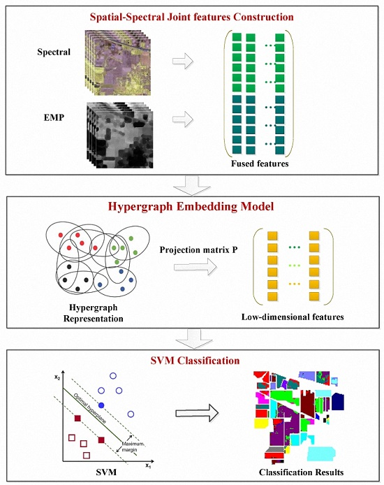
In order to cope with these issues, we propose a novel algorithm for HSI spatial-spectral joint feature extraction. We combine the EMP and spectral features and adopt the KNN method to construct a hypergraph, where each sample and its K nearest neighbors are enclosed in one hyperedge. Similar to [36], a linear projection matrix P can be learnt by solving the hypergraph embedding model. However, in [36], the hyperedges’ weights in the hypergraph embedded model are fixed. Inspired by [39,40], we introduce a scheme to update the weights adaptively to preserve the prominent hyperedge and further learn the low-dimensional structure. It helps improve the accuracy of the final HSI classification to a certain extent. Finally, the leaned low-dimensional features are fed to the SVM for classification. The flowchart of the proposed method is shown in Figure 1. Experiments conducted on three widely used types of HSI demonstrate that the proposed method achieves superior performance over many other feature extract methods for HSI classification.
2. Hypergraph Model
Denote a hypergraph as , which consists of a set of vertices V, a family of hyperedge E and a weight matrix W of hyperedges. Different from pairwise graphs (For convenience, we call it a simple graph in the following), every hyperedge can contain multiple vertices and is assigned a weight . As shown in Figure 2b, hyperedge is composed of vertices , and . is composed of vertices and . is composed of vertices , , and . W is a diagonal matrix of the hyperedge weights. The connection relationship of hypergraph G can be represented by an incidence matrix , which can be defined as:
The degree of vertex v and hyperedge e can be respectively represented as:
According to the above definition, the main difference between hypergraphs and simple graphs is that every hyperedge can link more than two vertexes. Therefore, hypergraph is suitable to represent local group information and the high-order relationship of data. For example, considering seven vertices in Figure 2b, they are attributed to three groups and the corresponding incidence matrix is shown in Figure 2c. In terms of building a simple graph with these seven data points, the complex relations within the group are broken into multiple pairwise links. Some valuable information may be lost in this procedure; therefore, a simple graph can not describe the group structure well.
3. Hypergraph Embedding of Spatial-Spectral Joint Features
As shown in Figure 1, our algorithm mainly consists of three steps: spatial-spectral joint feature construction, hypergraph embedding and SVM classification.
3.1. Spatial-Spectral Joint Feature Construction
Following [16], we first extract several PCs from the original HSI and then build an MP from each of the PCs:
where n is the number of the circular structural element (SE) with different radius sizes, and are the opening profile (OP) and the closing profile (CP) at the pixel x with an SE of a size n, respectively. Specifically, we have . The MP of contains the original image , n opening profile and n closing profile. Therefore, each MP is a -dimensional vector. Finally, all MPs are stacked together in one as EMP:
where m represents the number of PCs. The EMP is defined as an -dimensional vector.
After obtaining the EMP feature, we represent the spatial and spectral joint feature of the i-th HSI pixel as
where d is the number of the spectral bands. Denote the spectral features matrix of HSI as , EMP matrix of HSI as , where is the i-th pixel, and N is the number of HSI pixels. Then, the joint feature matrix of HSI can be represented as: .
3.2. Hypergraph Embedding
We take each pixel of HSI as a vertex and construct a hypergraph to represent the correlation between HSI pixels. Each vertex is associated with the spatial and spectral joint feature defined in Equation (6). The hypergraph G is constructed by the K-nearest neighbor method. In detail, each pixel and its K nearest neighbors are enclosed as hyperedge . Thus, hyperedge set contains N hyperedges. Meanwhile, the weight of hyperedge is defined as:
where is the mean distance between all vertices and can be calculated by , is the distance between vertex and vertex . The degree of vertex and the degree of hyperedge can be computed by Equations (2) and (3), respectively. Based on this definition, the more "compact" hyperedge (local group) is assigned with a higher weight.
Denote and as two diagonal matrices of the vertex degrees and the hyperedge degrees, respectively, and (generally, ) as the linear projection matrix. The objective of hypergraph embedding model is to learn the projection matrix for reducing the feature dimension with the preservation of geometric property in the original space. The objective function is formulated as:
where is the hypergraph laplacian matrix. The constraint is used for scale normalization of the low-dimensional representations. This objective function induces the constraint that if and are similar and belong to the same hyperedge, they should also be adjacent in embedded space. In addition, an efficient hypergraph weight estimation scheme is proposed to preserve the prominent hyperedges. Assuming that is composed of the elements lying in the main diagonal of W, we enforce and add an norm regularizer on . Then, our proposed embedding model is finally defined as:
3.3. Optimization Algorithm
The objective function Equation (9) is a multiple variables optimization problem, and it is non-convex with respect to w and jointly. However, it is convex with either of them individually when the other is fixed. Thus, an alternative iteration strategy is adopted to get the solution of Equation (9). We first initialize w according to Equation (7). With w fixed, we optimize P according to Equation (8). The solution of Equation (8) is to find the eigenvectors corresponding to the first u largest eigenvalues of the matrix .
Next, fix P and optimize w:
In this paper, we employ the Lagrangian algorithm to optimize the Equation (10). The Lagrangian function of the objective function (10) is defined as:
The partial derivatives of w.r.t. are given by:
By simplifying Equation (12), can be calculated as:
According to the constraint , the Lagrange multiplier can be calculated as:
Following this iteration process, w and P are alternately optimized until the maximal iteration number is reached or the relative difference of objective function value of Equation (9) is smaller than a given tolerance const , i.e.,
where and is the function value of Equation (9) at iteration and t, respectively. In addition, we can obtain the final projection matrix . At last, the joint feature set is reduced as a low-dimensional feature set , which is then transmitted into an SVM classifier. Based on the above analysis, the proposed method can be summarized in Algorithm 1.
| Algorithm 1: The proposed method ( denoted as SSHG*) for HSI classification. |
|
4. Experiments and Discussion
4.1. Data Sets
In order to verify the performance of our proposed method, we conduct the experiments on the following three benchmark datasets.
- (1)
- Indian Pines data set—the first data set was acquired by the AVIRIS sensor over the Indian Pines test site in Northwestern Indiana, USA. The size of the image is 145 pixels × 145 pixels with a spatial resolution of 20 m per pixel. Twenty water absorption bands (104–108, 150–163, 220) were removed, and the 200-band image is used for experiments. Sixteen classes of interest are considered.
- (2)
- Pavia University data set—the second data set was acquired by the ROSIS sensor during a flight campaign over Pavia, northern Italy. The size of the image is 610 pixels × 340 pixels with a spatial resolution of 1.3 m per pixel. Twelve channels were removed due to noise. The remaining 103 spectral bands are processed. Nine classes of interest are considered.
- (3)
- Botswana data set—the third data set was acquired by the NASA EO-1 satellite over the Okavango Delta, Botswana, in 2001. The size of the image is 1476 pixels × 256 pixels with a spatial resolution of 30 m per pixel. Uncalibrated and noisy bands that cover water absorption features were removed, and the remaining 145 bands are used for experiment. Fourteen classes of interest are considered.
4.2. Experimental Setting
In order to demonstrate the effectiveness of adaptive weight estimation, we implement our algorithm as two versions. One is SSHG, which only utilizes the KNN hypergraph model for dimension reduction of the stacked feature set without adaptive weight estimation. The other is SSHG* shown in Algorithm 1. They are compared with the following feature extraction methods: (1) the method by using PCA to extract spectral features (denoted as PCA); (2) the method by using EMP features without dimension reduction (denoted as EMP); (3) the method [17] stacking the EMP and the spectral features as feature without dimension reduction (denoted as EMPSpe); and (4) the spatial hypergraph embedding method proposed in [36] (denoted as SH). In order to facilitate comparisons with these competing feature extraction methods, we adopt the overall accuracy (OA), the average accuracy (AA), the per-class accuracy and Kappa coefficient () to evaluate the classification performance. Furthermore, the SVM classifier with Gaussian kernel is adopted to classify all of the aforementioned feature data of these feature extraction methods. The grid search tool is used to select the parameters of the optimal penalty term and Gaussian kernel variance in SVM within the given sets and , respectively. The one-against-all strategy is adopted for multi-class classification. Regarding the three data sets, we select 15 samples from each class randomly to form a training set and the remaining samples are used as the test set. The training sample selection and the classification process are repeated ten times to reduce the bias induced by random sampling. We retain the average results. The parameters setting of SH is the same as the original paper [36]. With respect to our algorithm, the tolerance const is set as and the regularization parameter is set as 100. The number of nearest neighbors K is selected as 10, 15, 5 for Indian Pines, Pavia University and Botswana data sets, respectively.
4.3. Experimental Results
The classification results of various methods upon three types of HSI are reported in Table 1, Table 2 and Table 3, respectively. The best results are highlighted with bold fonts. The number in brackets corresponds to the optimal dimensionality of reduced features. Classification maps of these different approaches are shown in Figure 3, Figure 4 and Figure 5, respectively. According to the experimental results, our proposed method achieves the highest OA, AA, and among all of the competing methods, which shows the effectiveness of our feature extraction algorithm. The effectiveness of our SSHG method owes much to the hypergraph embedding of spatial and spectral joint features.
Comparing the EMP and EMPSpe method, we can find that EMPSpe method is always slightly better than EMP due to the fusion of EMP and spectral features for classification. As mentioned in [17], the stacked EMP and spectral features are transformed to low dimensional features by the decision boundary feature extraction (DBFE) and NWFE methods before classification. However, the DBFE and NWFE did not bring about the effective improvement of algorithm performance. SH utilized the hypergraph embedding model for feature reduction. Compared with PCA, the SH method has much better classification performance, which verifies the capacity of the hypergraph to capture the intrinsic complex relationships between HSI pixels. However, SH utilized only the spectral similarity for finding the nearest neighbors within a given spatial region. The superiority of SSHG over SH demonstrates that the embedding of EMP and spectral features is better for HSI classification. Specifically, our SSHG method can extract the rich spatial structures in the Pavia University data and achieve the maximum improvement upon this data. SSHG* obtains better classification results than SSHG, which demonstrates that adaptive hypergraph weight estimation is also beneficial for improving the classification accuracy.
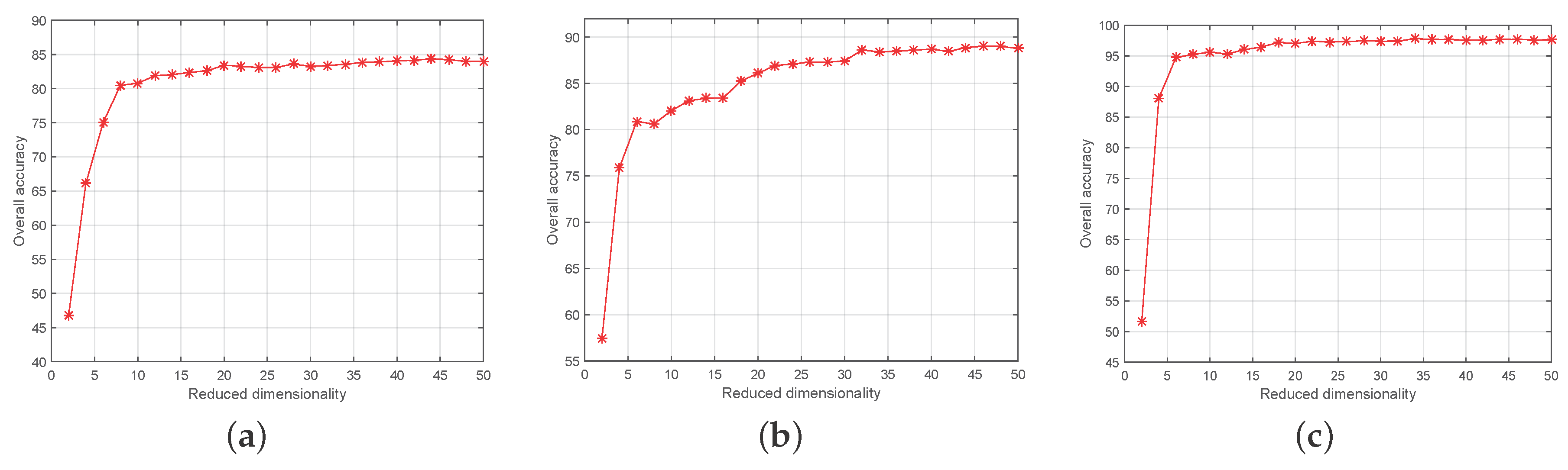
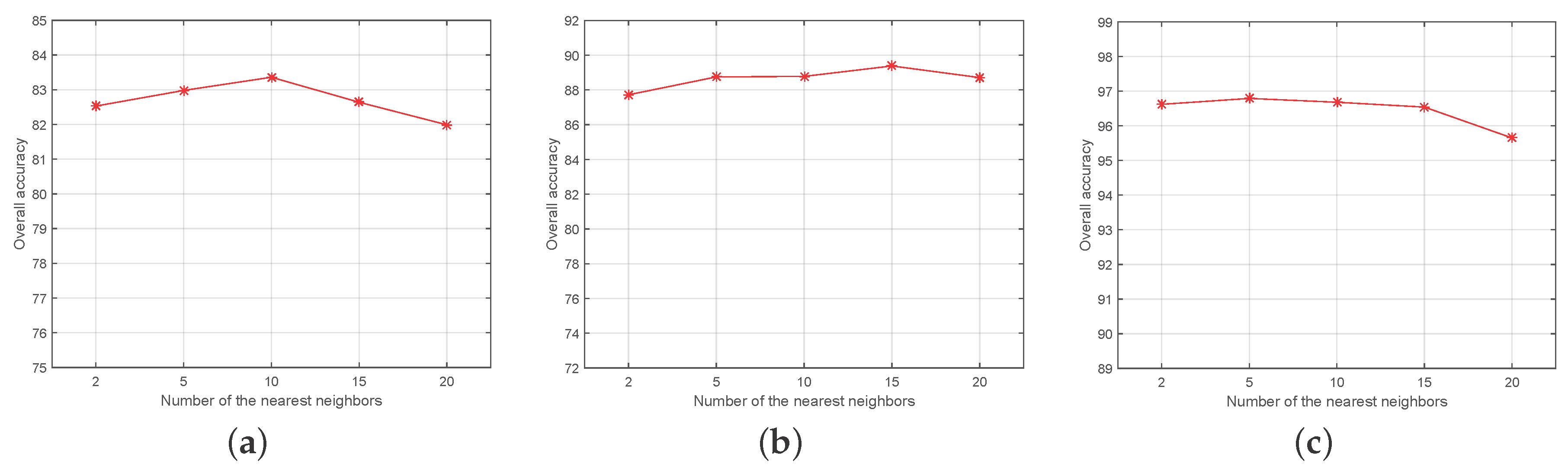
There are two parameters, i.e., K and u, in our proposed method. The parameter K is the number of nearest neighbors, which determines how many pixels are included in the hyperedge. u is the dimensionality of the embedded low-dimensional feature. To evaluate their effects on the classification performance, we conduct the experiments on the above three datasets. We firstly fix the reduced dimensionality as and evaluate the influence of different K on the OA. As seen in Figure 6, when K is set as 10, 15, 5 for Indian Pines, Pavia University and Botswana data sets, respectively, the OA achieves the highest value. Taken as a whole, is usually a good range for the selection of parameter K. We then fix the K as 10, 15, 5 for the three datasets, respectively, and evaluate the influence of different us on the OA. Figure 7 shows the changes of OA with the reduced dimensions on three types of HSI. We can see that the inflection point of classification results is around the dimensionality 25 for these three HSIs, and there was no significant improvement on the classification results if the dimension continues to grow up.
5. Conclusions
In this paper, we propose a novel algorithm for spatial-spectral feature extraction based on hypergraph learning. A hypergraph is constructed by the KNN method and the embedding operation is conducted to transform the joint EMP and spectral features into the low-dimensional representation. Meanwhile, an efficient hypergraph weight estimation scheme is adopted to preserve the prominent hyperedges. Classification is performed with SVM using the embedded features. The experimental results on three benchmark hyperspectral datasets verify that our embedded representation can enhance the classification accuracy effectively. The hypergraph weight estimation can further improve the accuracy of HSI classification.
Acknowledgments
This work was supported in part by the Natural Science Foundation of China under Grant Numbers: 61672292, 61532009, 61622305, 61502238, 61300162 and, in part, by the Six Talent Peaks Project of Jiangsu Province, China, under Grant DZXX-037.
Author Contributions
Yubao Sun and Sujuan Wang contributed equally to this work. They proposed the algorithm and performed the experiments. Qingshan Liu supervised the study, analyzed the results and gave insightful suggestions for the manuscript. Sujuan Wang and Yubao Sun drafted the manuscript. Guangcan Liu and Renlong Hang contributed to the revision of the manuscript. All authors read and approved the submitted manuscript.
Conflicts of Interest
The authors declare no conflict of interest.
References
- Clement, A. Advances in remote sensing of agriculture: context description, existing operational monitoring systems and major information needs. Remote Sens. 2013, 5, 949–981. [Google Scholar] [CrossRef]
- Shafri, H.Z.M.; Taherzadeh, E.; Mansor, S.; Ashurov, R. Hyperspectral remote sensing of urban areas: An overview of techniques and applications. Res. J. Appl. Sci. Eng. Technol. 2012, 4, 1557–1565. [Google Scholar]
- Abbate, G.; Fiumi, L.; De Lorenzo, C.; Vintila, R. Avaluation of remote sensing data for urban planning. Applicative examples by means of multispectral and hyperspectral data. In Proceedings of the GRSS/ISPRS Joint Workshop on Remote Sensing and Data Fusion over Urban Areas, Berlin, Germany, 22–23 May 2003; pp. 201–205. [Google Scholar]
- Wu, Z.; Wang, Q.; Plaza, A.; Li, J.; Sun, L. Parallel spatial-spectral hyperspectral image classification with sparse representation and markov random fields on GPUs. IEEE J. Sel. Top. Appl. Earth Obs. Remote Sens. 2015, 8, 2926–2938. [Google Scholar] [CrossRef]
- Yuan, Y.; Lin, J.; Wang, Q. Hyperspectral image classification via multitask joint sparse representation and stepwise MRF optimization. IEEE Trans. Cybern. 2016, 46, 2966–2977. [Google Scholar] [CrossRef] [PubMed]
- Wang, Q.; Lin, J.; Yuan, Y. Salient band selection for hyperspectral image classification via manifold ranking. IEEE IEEE Trans. Neural Netw. Learn. Syst. 2016, 27, 1279–1289. [Google Scholar] [CrossRef] [PubMed]
- Hang, R.; Liu, Q.; Sun, Y.; Yuan, X.; Pei, H.; Plaza, J.; Plaza, A. Robust matrix discriminative analysis for feature extraction from hyperspectral images. IEEE J. Sel. Top. Appl. Earth Obs. Remote Sens. 2017, 10, 2002–2011. [Google Scholar] [CrossRef]
- Wu, Z.; Li, Y.; Plaza, A.; Li, J.; Xiao, F.; Wei, Z. Parallel and distributed dimensionality reduction of hyperspectral data on cloud computing architectures. IEEE J. Sel. Top. Appl. Earth Obs. Remote Sens. 2016, 9, 2270–2278. [Google Scholar] [CrossRef]
- Sun, Y.; Hang, R.; Liu, Q.; Zhu, F.; Pei, H. Graph-Regularized low rank representation for aerosol optical depth retrieval. Int. J. Remote Sens. 2016, 37, 5749–5762. [Google Scholar] [CrossRef]
- Fauvel, M.; Tarabalka, Y.; Benediktsson, J.A.; Chanussot, J.; Tilton, J.C. Advances in spectral-spatial classification of hyperspectral images. Proc. IEEE 2013, 101, 652–675. [Google Scholar] [CrossRef]
- Yuan, Y.; Lin, J.; Wang, Q. Dual-Clustering-Based hyperspectral band selection by contextual analysis. IEEE Trans. Geosci. Remote Sens. 2016, 54, 1431–1445. [Google Scholar] [CrossRef]
- Kettig, R.L.; Landgrebe, D.A. Classification of multispectral image data by extraction and classification of homogeneous objects. IEEE Trans. Geosci. Electron. 1976, 14, 19–26. [Google Scholar] [CrossRef]
- Descombes, X.; Sigelle, M.; Preteu, F. GMRF parameter estimation in a non-stationary framework by a renormalization technique: application to remote sensing imaging. IEEE Trans. Image Process. 1999, 8, 490–503. [Google Scholar] [CrossRef] [PubMed]
- Jackson, Q.; Landgrebe, D.A. Adaptive bayesian contextual classification based on markov random fields. IEEE Trans. Geosci. Remote Sens. 2002, 40, 2454–2463. [Google Scholar] [CrossRef]
- Pesaresi, M.; Benediktsson, J.A. A new approach for the morphological segmentation of high-resolution satellite imagery. IEEE Trans. Geosci. Remote Sens. 2001, 39, 309–320. [Google Scholar] [CrossRef]
- Benediktsson, J.A.; Palmason, J.A.; Sveinsson, J.R. Classification of hyperspectral data from urban areas based on extended morphological profiles. IEEE Trans. Geosci. Remote Sens. 2005, 43, 480–491. [Google Scholar] [CrossRef]
- Fauvel, M.; Benediktsson, J.A.; Chanussot, J.; Sveinsson, J.R. Spectral and spatial classification of hyperspectral data using svms and morphological profiles. IEEE Trans. Geosci. Remote Sens. 2008, 46, 3804–3814. [Google Scholar] [CrossRef]
- Guo, X.; Huang, X.; Zhang, L. Three-Dimensional wavelet texture feature extraction and classification for multi/hyperspectral imagery. IEEE Geosci. Remote Sens. Lett. 2014, 11, 2183–2187. [Google Scholar] [CrossRef]
- Li, L.; Marpu, P.R.; Plaza, A.; Bioucas-Dias, J.M. Generalized composite kernel framework for hyperspectral image classification. IEEE Trans. Geosci. Remote Sens. 2013, 51, 4816–4829. [Google Scholar] [CrossRef]
- Hang, R.; Liu, Q.; Song, H.; Sun, Y. Matrix-based discriminant subspace ensemble for hyperspectral image spatial–spectral feature fusion. IEEE Trans. Geosci. Remote Sens. 2016, 54, 783–794. [Google Scholar] [CrossRef]
- Fang, L.; Li, S.; Kang, X.; Benediktsson, J.A. Spectral-spatial hyperspectral image classification via multiscale adaptive sparse representation. IEEE Trans. Geosci. Remote Sens. 2014, 52, 7738–7749. [Google Scholar] [CrossRef]
- Chen, Y.; Lin, Z.; Zhao, X.; Wang, G.; Gu, Y. Deep learning-based classification of hyperspectral data. IEEE J. Sel. Top. Appl. Earth Obs. 2014, 7, 2094–2107. [Google Scholar] [CrossRef]
- Du, Q. Modified fisher’s linear discriminant analysis for hyperspectral imagery. IEEE Geosci. Remote Sens. Lett. 2007, 4, 503–507. [Google Scholar] [CrossRef]
- Fauvel, M.; Chanussot, J.; Benediktsson, J.; Atli, N. Kernel principal component analysis for the classification of hyperspectral remote sensing data over urban areas. EURASIP J. Adv. Signal Process. 2009, 2009, 1–14. [Google Scholar] [CrossRef]
- Li, W.; Prasad, S.; Fowler, J.E. Decision fusion in kernel-induced spaces for hyperspectral image classification. IEEE Trans. Geosci. Remote Sens. 2014, 52, 3399–3411. [Google Scholar] [CrossRef]
- He, X.; Niyogi, P. Locality preserving projections. In Proceedings of the Advances in Neural Information Processing Systems (NIPS), Vancouver, BC, Canada, 8–13 December 2003; pp. 186–197. [Google Scholar]
- Villa, A.; Benediktsson, J.A.; Chanussot, J.; Jutten, C. Hyperspectral image classification with independent component discriminant analysis. IEEE Trans. Geosci. Remote Sens. 2011, 49, 4865–4876. [Google Scholar] [CrossRef]
- Mura, M.D.; Villa, A.; Benediktsson, J.A.; Chanussot, J. Classification of hyperspectral images by using extended morphological attribute profiles and independent component analysis. IEEE Geosci. Remote Sens. Lett. 2011, 8, 542–546. [Google Scholar] [CrossRef]
- Roweis, S.T.; Saul, L.K. Nonlinear dimensionality reduction by locally linear embedding. Science 2000, 290, 2323–2326. [Google Scholar] [CrossRef] [PubMed]
- Yan, S.; Xu, D.; Zhang, B.; Zhang, H.J. Graph embedding and extensions: A general framework for dimensionality reduction. IEEE Trans. Pattern Anal. Mach. Intell. 2007, 29, 40–51. [Google Scholar] [CrossRef] [PubMed]
- Luo, F.; Huang, H.; Liu, J.; Ma, Z. Fusion of graph embedding and sparse representation for feature extraction and classification of hyperspectral imagery. Photogramm. Eng. Remote Sens. 2017, 83, 37–46. [Google Scholar] [CrossRef]
- Chen, P.; Jiao, L.; Liu, F.; Zhao, J.; Zhao, Z. Dimensionality reduction for hyperspectral image classification based on multiview graphs ensemble. J. Appl. Remote Sens. 2016, 10, 030501. [Google Scholar] [CrossRef]
- Zhou, D.; Huang, J.; Schölkopf, B. Learning with hypergraphs: clustering, classification, and embedding. In Proceedings of the Advances in Neural Information Processing Systems, Vancouver, BC, Canada, 3–6 December 2007; pp. 1601–1608. [Google Scholar]
- Bu, J.; Tan, S.; Chen, C.; Wang, C.; Wu, H.; Zhang, L.; He, X. Music recommendation by unified hypergraph: combining social media information and music content. In Proceedings of the 18th ACM international conference on Multimedia, Firenze, Italy, 25–29 October 2010; pp. 391–400. [Google Scholar]
- Liu, Q.; Sun, Y.; Wang, C.; Liu, T.; Tao, D. Elastic net hypergraph learning for image clustering and semi-supervised classification. IEEE Trans. Image Process. 2017, 26, 452–463. [Google Scholar] [CrossRef] [PubMed]
- Yuan, H.; Tang, Y.Y. Learning with hypergraph for hyperspectral image feature extraction. IEEE Trans. Geosci. Remote Sens. Lett. 2015, 12, 1695–1699. [Google Scholar] [CrossRef]
- Kuo, B.C.; Landgrebe, D.A. Nonparametric weighted feature extraction for classification. IEEE Trans. Geosci. Remote Sens. 2004, 42, 1096–1105. [Google Scholar] [CrossRef]
- Liao, W.; Pizurica, A.; Scheunders, P.; Philips, W.; Pi, Y. Semisupervised local discriminant analysis for feature extraction in hyperspectral images. IEEE Trans. Geosci. Remote Sens. 2013, 51, 184–198. [Google Scholar] [CrossRef]
- Pliakos, K.; Kotropoulos, C. Weight estimation in hypergraph learning. In Proceedings of the IEEE International Conference on Acoustics, Speech and Signal Processing, South Brisbane, Australia, 19–24 April 2015; pp. 1161–1165. [Google Scholar]
- Gao, Y.; Wang, W.; Zha, Z.J.; Shen, J.; Li, X.; Wu, X. Visual-textual joint relevance learning for tag-based social image search. IEEE Trans. Image Process. 2013, 22, 363–376. [Google Scholar] [CrossRef] [PubMed]
Figure 1.
The flowchart of the proposed method.

Figure 2.
The example of graph and hypergraph (a) simple graph, each edge consists of only two data points; (b) hypergraph G, each hyperedge is marked by an ellipse and consists of at least two data points; (c) taking the seven vertices as example, H is the incidence matrix of G, whose values are usually binary.
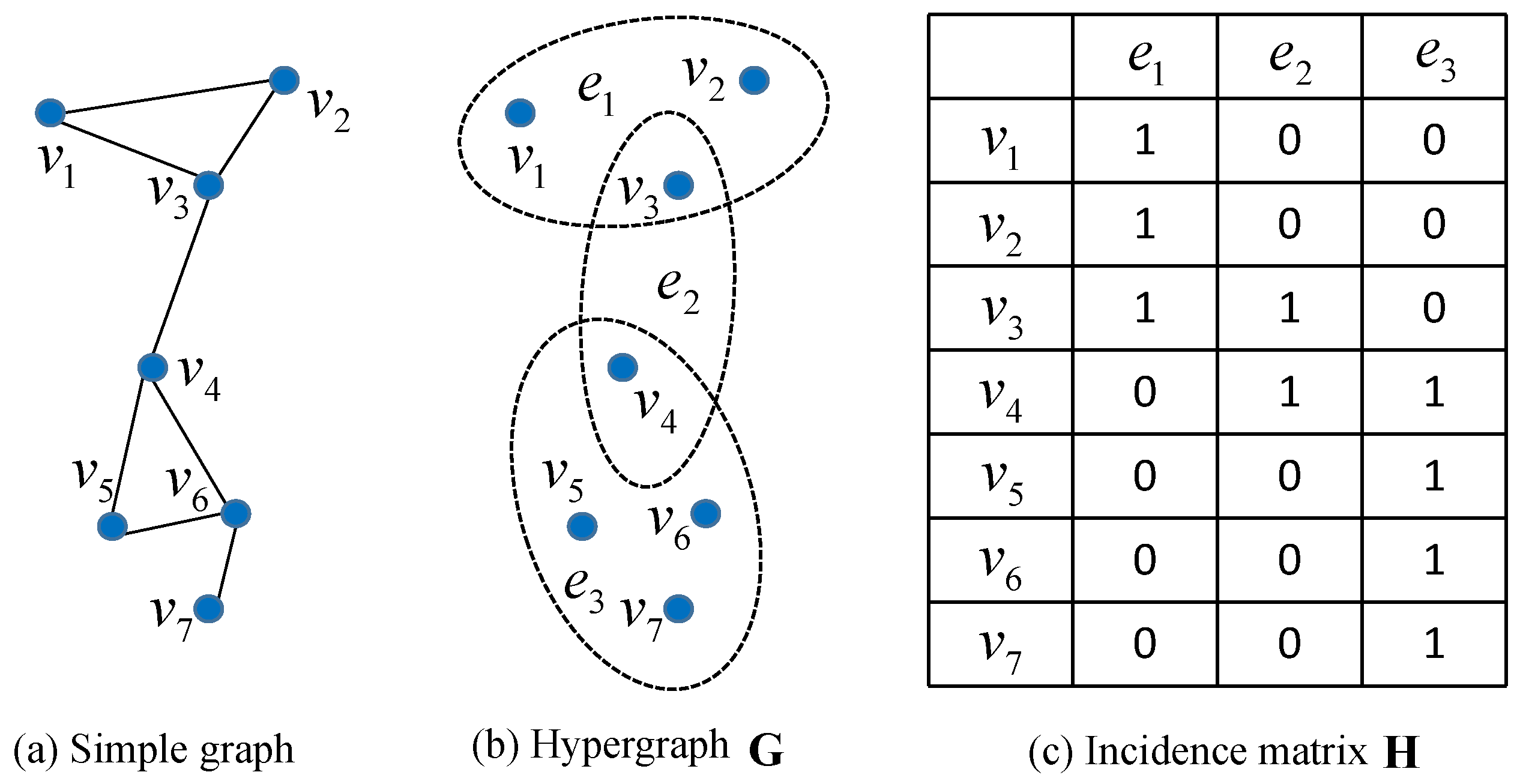
Figure 3.
Indian Pines. (a) three-channel color composite image with bands 65, 52, 36; (b,c) ground-truth map and class labels; (d–i) classification maps of PCA, EMP, EMPSpe, SH, SSHG, SSHG*, respectively.
Figure 3.
Indian Pines. (a) three-channel color composite image with bands 65, 52, 36; (b,c) ground-truth map and class labels; (d–i) classification maps of PCA, EMP, EMPSpe, SH, SSHG, SSHG*, respectively.
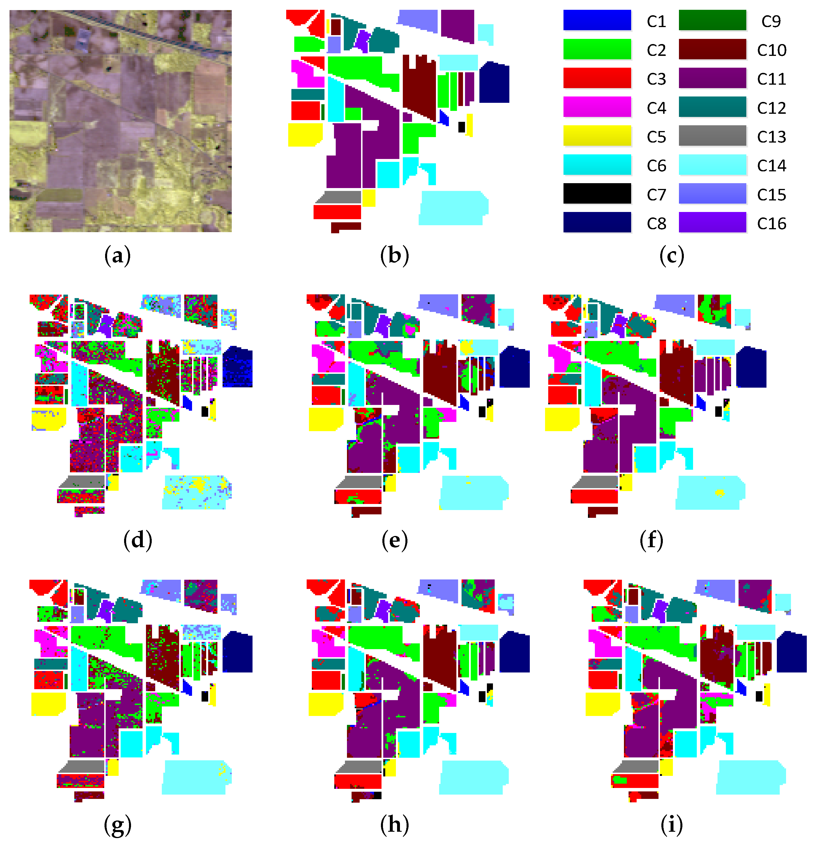
Figure 4.
Pavia university. (a) three-channel color composite image with bands 102, 56, 31; (b,c) ground-truth map and class labels; (d–i) classification maps of PCA, EMP, EMPSpe, SH, SSHG, SSHG*, respectively.
Figure 4.
Pavia university. (a) three-channel color composite image with bands 102, 56, 31; (b,c) ground-truth map and class labels; (d–i) classification maps of PCA, EMP, EMPSpe, SH, SSHG, SSHG*, respectively.
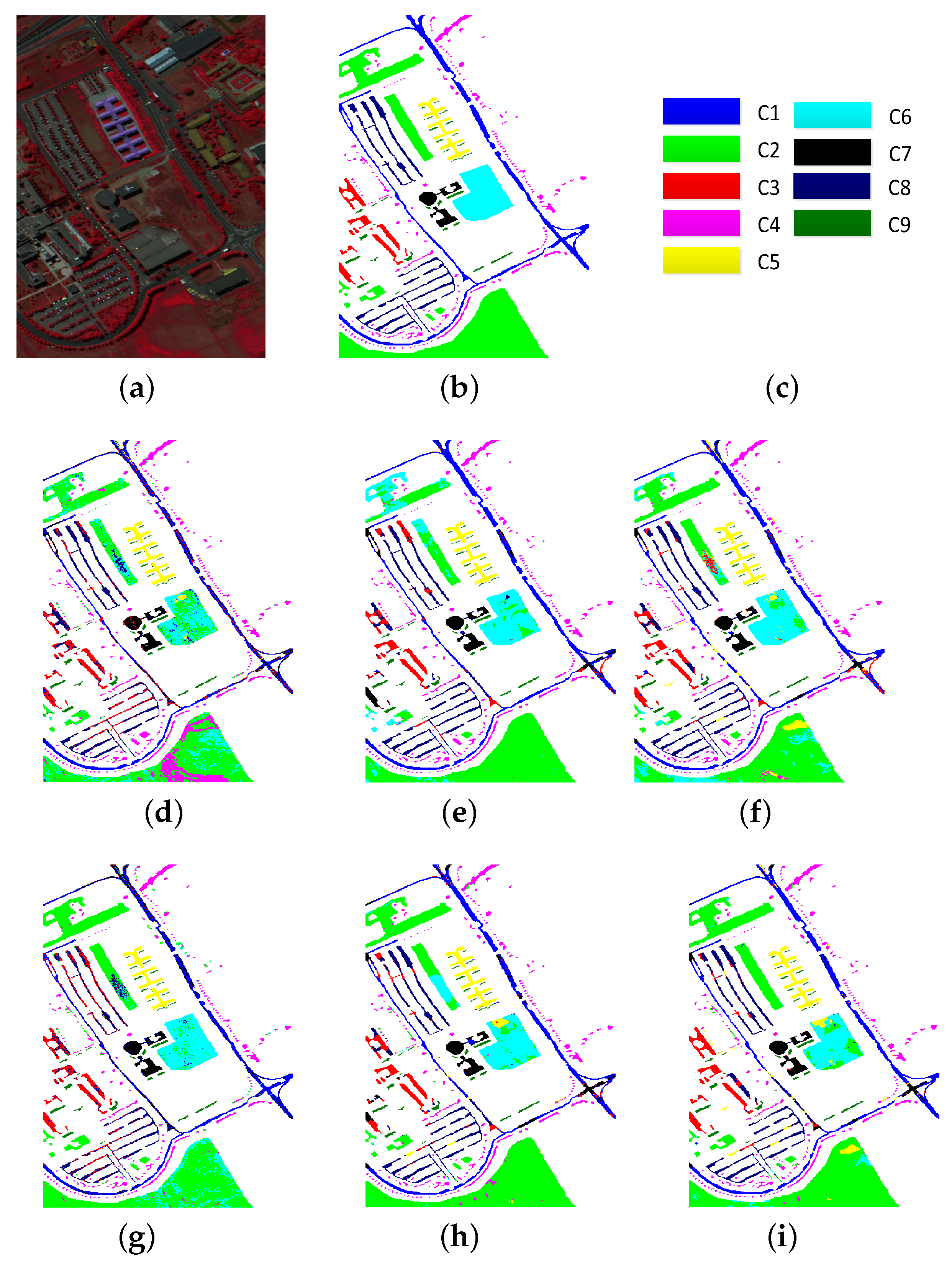
Figure 5.
Botswana. (a) three-channel color composite image with bands 65, 52, 36; (b,c) ground-truth map and class labels; (d–i) classification maps of PCA, EMP, EMPSpe, SH, SSHG, SSHG*, respectively.
Figure 5.
Botswana. (a) three-channel color composite image with bands 65, 52, 36; (b,c) ground-truth map and class labels; (d–i) classification maps of PCA, EMP, EMPSpe, SH, SSHG, SSHG*, respectively.
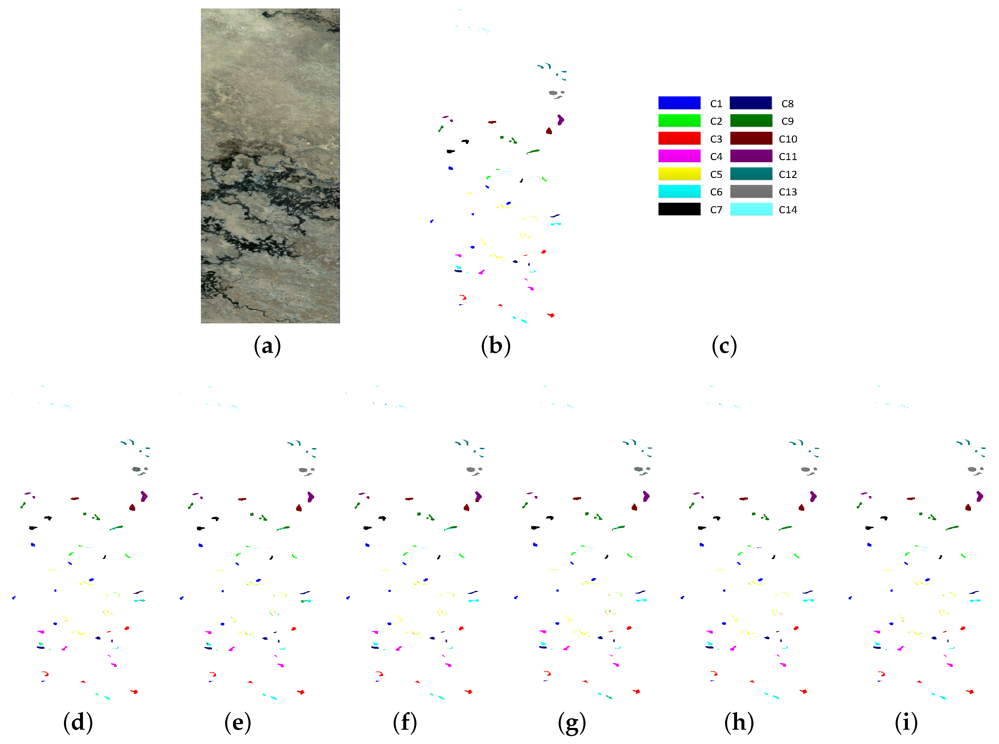
Figure 6.
Effects of the number K of nearest neighbors on OA. (a) Indian Pines; (b) Pavia University; (c) Botswana.
Figure 6.
Effects of the number K of nearest neighbors on OA. (a) Indian Pines; (b) Pavia University; (c) Botswana.

Figure 7.
Effects on the reduced dimensions. (a) Indian Pines; (b) Pavia University; (c) Botswana.

Table 1.
Classification accuracy of various algorithms on the Indian Pines image.
| Class | PCA (25) | EMP (27) | EMPSpe (227) | SH (22) | SSHG (44) | SSHG* (44) |
|---|---|---|---|---|---|---|
| 1 | 91.61 | 98.71 | 99.03 | 94.87 | 98.06 | 98.06 |
| 2 | 47.36 | 61.46 | 64.28 | 82.59 | 72.53 | 73.96 |
| 3 | 48.60 | 78.75 | 77.14 | 73.50 | 84.06 | 84.85 |
| 4 | 68.29 | 95.90 | 91.76 | 91.32 | 96.76 | 97.21 |
| 5 | 75.75 | 87.78 | 88.85 | 92.12 | 89.83 | 90.32 |
| 6 | 85.37 | 91.48 | 92.36 | 98.22 | 93.93 | 94.04 |
| 7 | 91.54 | 99.23 | 99.23 | 100 | 100 | 100 |
| 8 | 79.52 | 98.47 | 98.92 | 98.31 | 99.57 | 99.63 |
| 9 | 96.00 | 100 | 100 | 100 | 100 | 100 |
| 10 | 56.22 | 74.23 | 71.61 | 87.51 | 76.81 | 77.68 |
| 11 | 49.62 | 69.51 | 71.02 | 64.41 | 75.65 | 75.57 |
| 12 | 45.43 | 75.67 | 77.40 | 84.31 | 84.33 | 84.79 |
| 13 | 93.47 | 98.68 | 99.00 | 99.49 | 99.37 | 99.37 |
| 14 | 69.55 | 93.25 | 94.83 | 94.84 | 97.57 | 97.58 |
| 15 | 46.42 | 95.96 | 95.85 | 75.07 | 97.74 | 97.76 |
| 16 | 89.62 | 97.56 | 98.46 | 98.75 | 99.74 | 99.87 |
| OA | 58.90 | 79.14 | 79.88 | 82.33 | 84.36 | 84.75 |
| AA | 70.90 | 88.54 | 88.73 | 89.71 | 91.62 | 91.92 |
| kappa | 53.88 | 76.42 | 77.24 | 80.06 | 82.27 | 82.73 |
Table 2.
Classification accuracy of various algorithms on the Pavia university image.
| Class | PCA (10) | EMP (27) | EMPSpe (130) | SH (30) | SSHG (46) | SSHG* (46) |
|---|---|---|---|---|---|---|
| 1 | 66.21 | 82.40 | 81.57 | 70.33 | 81.67 | 82.70 |
| 2 | 65.14 | 83.44 | 84.09 | 82.13 | 92.02 | 91.44 |
| 3 | 70.00 | 77.04 | 77.79 | 72.37 | 80.47 | 80.08 |
| 4 | 85.26 | 97.42 | 97.44 | 89.58 | 93.93 | 94.90 |
| 5 | 99.37 | 99.76 | 99.75 | 99.61 | 99.79 | 99.80 |
| 6 | 69.16 | 78.91 | 80.16 | 91.76 | 86.50 | 89.63 |
| 7 | 90.45 | 94.07 | 93.28 | 92.68 | 94.16 | 94.44 |
| 8 | 71.34 | 86.12 | 85.30 | 72.16 | 83.07 | 84.06 |
| 9 | 99.72 | 96.04 | 97.44 | 99.51 | 98.26 | 98.15 |
| OA | 70.59 | 84.77 | 85.05 | 81.88 | 89.01 | 89.43 |
| AA | 79.63 | 88.35 | 88.53 | 85.57 | 89.99 | 90.58 |
| kappa | 63.20 | 80.38 | 80.78 | 76.80 | 85.64 | 86.24 |
Table 3.
Classification accuracy of various algorithms on the Botswana image.
| Class | PCA (22) | EMP (27) | EMPSpe (172) | SH (25) | SSHG (34) | SSHG* (34) |
|---|---|---|---|---|---|---|
| 1 | 100 | 99.92 | 99.89 | 100 | 100 | 100 |
| 2 | 96.51 | 100 | 97.99 | 100 | 99.68 | 98.05 |
| 3 | 96.19 | 94.79 | 95.85 | 99.15 | 96.76 | 100 |
| 4 | 99.00 | 95.85 | 98.83 | 99.50 | 98.41 | 93.27 |
| 5 | 81.10 | 79.76 | 82.32 | 82.86 | 91.79 | 96.38 |
| 6 | 69.29 | 81.73 | 88.34 | 81.89 | 96.37 | 99.22 |
| 7 | 96.31 | 97.70 | 99.20 | 98.77 | 99.72 | 99.95 |
| 8 | 98.40 | 99.63 | 99.48 | 99.47 | 100 | 97.42 |
| 9 | 79.93 | 92.34 | 94.47 | 96.32 | 98.86 | 99.79 |
| 10 | 95.28 | 98.33 | 97.98 | 99.57 | 99.92 | 97.97 |
| 11 | 83.45 | 97.24 | 95.19 | 97.59 | 94.97 | 99.88 |
| 12 | 93.98 | 99.94 | 99.88 | 88.55 | 100 | 99.49 |
| 13 | 89.33 | 99.60 | 98.37 | 94.47 | 99.92 | 99.75 |
| 14 | 98.75 | 99.25 | 98.35 | 100 | 91.36 | 99.63 |
| OA | 89.83 | 94.69 | 95.65 | 95.10 | 97.79 | 98.38 |
| AA | 91.25 | 95.43 | 96.15 | 95.58 | 97.70 | 98.63 |
| kappa | 88.98 | 94.24 | 95.36 | 94.68 | 97.60 | 98.24 |
© 2017 by the authors. Licensee MDPI, Basel, Switzerland. This article is an open access article distributed under the terms and conditions of the Creative Commons Attribution (CC BY) license (http://creativecommons.org/licenses/by/4.0/).
Share and Cite
MDPI and ACS Style
Sun, Y.; Wang, S.; Liu, Q.; Hang, R.; Liu, G. Hypergraph Embedding for Spatial-Spectral Joint Feature Extraction in Hyperspectral Images. Remote Sens. 2017, 9, 506. https://doi.org/10.3390/rs9050506
AMA Style
Sun Y, Wang S, Liu Q, Hang R, Liu G. Hypergraph Embedding for Spatial-Spectral Joint Feature Extraction in Hyperspectral Images. Remote Sensing. 2017; 9(5):506. https://doi.org/10.3390/rs9050506
Chicago/Turabian StyleSun, Yubao, Sujuan Wang, Qingshan Liu, Renlong Hang, and Guangcan Liu. 2017. "Hypergraph Embedding for Spatial-Spectral Joint Feature Extraction in Hyperspectral Images" Remote Sensing 9, no. 5: 506. https://doi.org/10.3390/rs9050506
Note that from the first issue of 2016, this journal uses article numbers instead of page numbers. See further details here.