Review

Annual and Seasonal Glacier-Wide Surface Mass Balance Quantified from Changes in Glacier Surface State: A Review on Existing Methods Using Optical Satellite Imagery

1
Univ. Grenoble Alpes, CNRS, IRD, Institut des Géosciences de l’Environnement (IGE), F-38000 Grenoble, France
2
National School of Surveying, University Otago, Dunedin 9054, New Zealand
3
Univ. Toulouse, CNES, CNRS, IRD, Laboratoire d’études en géophysiques et océanographie spatiales (LEGOS), F-31000 Toulouse, France
4
Météo-France, CNRS, Centre national de recherches météorologiques/Centre d’études de la neige (CNRM/CEN), F-38000 Grenoble, France
*
Author to whom correspondence should be addressed.
Remote Sens. 2017, 9(5), 507; https://doi.org/10.3390/rs9050507
Submission received: 23 February 2017 / Revised: 11 May 2017 / Accepted: 16 May 2017 / Published: 20 May 2017
(This article belongs to the Special Issue Remote Sensing of Glaciers)

Abstract

:
Glaciers are one of the terrestrial essential climate variables (ECVs) as they respond very sensitively to climate change. A key driver of their response is the glacier surface mass balance that is typically derived from field measurements. It deserves to be quantified over long time scales to better understand the accumulation and ablation processes at the glacier surface and their relationships with inter-annual changes in meteorological conditions and long-term climate changes. Glaciers with in situ monitoring of surface mass balance are scarce at the global scale, and satellite remote sensing provides a powerful tool to increase the number of monitored glaciers. In this study, we present a review of three optical remote sensing methods developed to quantify seasonal and annual glacier surface mass balances. These methodologies rely on the multitemporal monitoring of the end-of-summer snow line for the equilibrium-line altitude (ELA) method, the annual cycle of glacier surface albedo for the albedo method and the mapping of the regional snow cover at the seasonal scale for the snow-map method. Together with a presentation of each method, an application is illustrated. The ELA method shows promising results to quantify annual surface mass balance and to reconstruct multi-decadal time series. The other two methods currently need a calibration on the basis of existing in situ data; however, a generalization of these methods (without calibration) could be achieved. The two latter methods show satisfying results at the annual and seasonal scales, particularly for the summer surface mass balance in the case of the albedo method and for the winter surface mass balance in the case of the snow-map method. The limits of each method (e.g., cloud coverage, debris-covered glaciers, monsoon-regime and cold glaciers), their complementarities and the future challenges (e.g., automating of the satellite images processing, generalization of the methods needing calibration) are also discussed.

1. Introduction

Glaciers and ice caps are one of the 50 essential climate variables recognized by the Global Climate Observing System (GCOS), an internationally-coordinated network of observing systems designed to meet evolving national and international requirements for climate observations [1]. Among the main glacier characteristics (e.g., length, surface area, mass balance), the surface mass balance (SMB) is the most relevant in terms of climate, as it is governed by the processes of accumulation and ablation at the glacier surface, primarily driven by the atmospheric conditions.
Logistical, human and financial constraints associated with field measurements result in a comparably small number of glaciers being permanently monitored in different climate regions worldwide. Regarding the SMB, the World Glacier Monitoring Service (WGMS) lists data available for 440 glaciers monitored worldwide through direct field measurements, including uninterrupted series longer than 40 years, for only 40 glaciers [2]. The 440 monitored glaciers represent only 0.25% of the nearly 200,000 glaciers inventoried on Earth and included in the Randolph Glacier Inventory (RGI) and GLIMS databases [3,4]. This small sample limits our understanding of the relationship between climate and glacier changes at regional to global scales, as well as our understanding of the contribution of glaciers to water resources and to the biodiversity of high-altitude watersheds.
Consequently, there is a need for monitoring approaches that are complementary to field measurements to quantify the SMB of individual glaciers at a regional scale. For this purpose, satellite remote sensing has proven to be a very useful tool. The increase in the number and availability of satellite sensors over nearly four decades, as well as their improved performance, i.e., their improved spatial, radiometric and temporal resolutions, has made remote sensing approaches vital for the monitoring of glaciers. Many remote sensing methods have been developed since the 1970s to determine the physical characteristics of glaciers (e.g., [5]). While variables such as length and areal extent, as well as their variations, could be retrieved relatively easily from sparse or intermittent imagery, the increase of satellite stereo imagery and advances in space-borne photogrammetry have allowed glacier topography to be repeatedly mapped and, in turn, geodetic mass balance to be derived. For example, digital elevation models (DEMs) can be derived from medium-to-high resolution optical satellite images (e.g., SPOT-5/HRS or ASTER) images or radar satellite data (e.g., SRTM), but the vertical precision (~5 m) prevents an accurate estimation of the mass balance of individual glaciers typically smaller than ~10 km2. New generations of satellites sub-metric optical stereo-images (e.g., Worldview, Pléiades) show promise to provide accurate glacier topography with a vertical precision of ±1 m and even ±0.5 m on gently-sloping glacier tongues and retrieve annual and seasonal glacier-wide SMB using the DEM differencing method (e.g., [6,7]). However, the deployment of this method at a regional scale is still hampered by the limited availability, footprint (e.g., 20 km × 20 km for Pléiades) and cost of these commercial stereo-images at the right time of the year. In addition, it is worth noting that the geodetic method needs a density value for the conversion from volume change to mass change. Because this value and its spatio-temporal variations at the glacier scale are hardly quantifiable, this method currently provides mass balance at a temporal resolution typically of five to ten years.
Alternatively, changes in the state of a glacier surface have been used to infer its surface mass balance. In particular, variations in the respective area of the accumulation zone and the ablation zone of glaciers via the mapping of the end-of-summer snow line support estimates of the equilibrium-line altitude (ELA) and/or the accumulation area ratio (AAR) that are used in turn to infer annual SMB. In this context, improvements and systematic application of the ELA method, as well as emerging approaches based on the regular monitoring of snow and ice surfaces have confirmed the potential to confidently estimate annual and seasonal SMB of glaciers (e.g., [8,9]). In this study, we present an overview of three remote sensing techniques developed recently to retrieve the annual and seasonal SMB of mountain glaciers using optical satellite images of high (SPOT, Landsat, ASTER), medium (MODIS) and low (SPOT/VGT, Proba-V) resolution. These methods share a common theme, which is to characterize the state of the glacier surface (i.e., snow line altitude, glacier surface albedo, seasonal snow cover) and its spatio-temporal changes.
Each of the three methods is presented in Section 2 with an application. Section 3 discusses the limits and complementarities of the methods, as well as the future challenges together with possible further improvements.

2. Methods to Retrieve Annual and Seasonal Glacier-Wide Surface Mass Balances Using Optical Satellite Imagery

In order to simplify the text, the method using the snow line detection as a proxy of the ELA from high resolution optical satellite images is called the “ELA method”; the one that uses the quantification of the glacier-wide surface albedo from medium resolution optical satellite images is called the “albedo method”; and the one that uses the mapping of the average regional snow cover extent from low resolution optical satellite images is called the “snow-map method”.

2.1. The ELA method

2.1.1. Principles and History of the Method

For glaciers where the formation of superimposed ice [10] is negligible, it is commonly accepted that the position of the glacier snow line at the end of the ablation season is representative of the equilibrium line [11]. Indeed, in the glacier reaches located above the altitude of the end-of-summer snow line, accumulation is greater than the ablation, and this part therefore constitutes the accumulation zone. Conversely, in the glacier reaches located below the altitude of the end-of-summer snow line, ablation is greater than the accumulation, and this part therefore constitutes the ablation zone. Thus, the SMB at the altitude of the end-of-summer snow line is zero, and the snow line therefore matches the equilibrium line. Moreover, at the annual scale, the altitude of the equilibrium line (ELA) exhibits high correlation with the SMB (e.g., [12,13,14]).
The potential for mapping the end-of-summer snow line in glaciological studies was considered as early as the 1950s–1960s based on aerial photographs [15,16], then since the early 1970s using the first civilian optical satellite imagery [17].
In the early 1980s, Braithwaite used in situ measurements of glacier SMB and ELA to propose a method to quantify the glacier SMB from its equilibrium line [12]. The method was based on the altitude difference between the ELA for a given year and the balance-budget ELA (called ELA0 and assumed to be constant by Braithwaite). To compute the annual SMB of the considered year, this difference is multiplied by the “effective balance gradient”, which represents a time- and space-average of the SMB gradient with altitude; a value considered constant by Braithwaite for a given region. Braithwaite yet recognized that there are large regional variations of the “effective balance gradient” and pointed out the potential error of using a universal value. Moreover, Braithwaite postulated that this value is representative of the mass balance gradient. However, when compared with measured SMB gradients available today, one can note that Braithwaite’s “effective balance gradient” values were 2–7-times higher than the SMB gradients.
Building upon these pioneering works by Braithwaite, a method to quantify the glacier SMB from the equilibrium line has been developed with the idea to be applied with remote-sensing data only, thus without any reliance on in situ measurements [13,18,19,20]. This method has been validated for mid-latitudes alpine glaciers [13,20] and glaciers in the outer tropics [21].
It is worth noting that other studies took advantage of the detection of the end-of-summer snow line from airborne or satellite data to document its year-to-year variability [22] or the changes in altitude of the snow line over the summer period as a proxy of ablation [23]. Other studies quantified the annual glacier-wide SMB by combining the altitude of end-of-summer snow line with the glacier hypsography and the SMB gradients above and below the ELA [24], or with a temperature-index model [25]. The method proposed by Shea et al. [24] depends on the availability of the SMB gradients in the ablation and accumulation zones, and uncertainties associated with these gradients and their use to compute the glacier-wide SMB can lead to significant errors. On the other hand, the method proposed by Tawde et al. [25] uses meteorological data and therefore depends on their availability in the vicinity of the studied glaciers. In this method, the errors related to the extrapolation of the meteorological variables can significantly affect the computed SMB.
The strength of the method proposed by Rabatel et al. [13] is due to the combination of the geodetic method and the temporal changes in the ELA. The geodetic method using DEM differencing ensures an accurate quantification of the changes in glacier mass over the entire study period (i.e., the value of the glacier-wide average annual SMB), and the changes in the ELA allow computing the annual departure in the glacier-wide SMB from its average computed by the geodetic method. In addition, in Rabatel et al. [13], the value used for the SMB gradient is the one in the vicinity of the ELA, i.e., in an elevation range where assuming this gradient as a constant over time and space is reasonable. Note that this assumption is also supported by Mernild et al. [23].
Consequently, in the method described in Rabatel et al. [13], the glacier-wide annual SMB series is reconstructed in two steps. First, for each year, the difference between altitude of the snow line at the end of the ablation season, SLAi (in m, used as a surrogate of ELAi), and the theoretical altitude of the equilibrium line if the glacier had a balanced budget (glacier wide mass balance = 0) over the study period, ELAeq (in m), is calculated. ELAeq is computed as:
E L A e q = 1 n 1 n ( S L A i ) + B ¯ b / z ,
where B ¯ is the average glacier-wide annual SMB over the study period (in m w.e. year−1) quantified by the DEM differencing method and ∂b/∂z is the SMB gradient in the vicinity of the ELA. This gradient, estimated from in situ data, is assumed constant across a glacierized region, for example 0.78 m w.e. 100 m−1 for the French Alps according to Rabatel et al. [13]. Rabatel et al. [13] demonstrated that even if ∂b/∂z for a specific glacier departs slightly from this value, using an average value at a regional scale does not compromise the results. The glacier-wide annual SMB Ba (in m w.e. year−1), computed for each year over the study period can then be expressed as:
B a = ( E L A e q S L A i ) × b z .
Applying the ELA method requires the following:
  • Two DEMs covering the entire region of interest (RoI); one at (or close to) the beginning of the study period, one at (or close to) the end.
  • One cloud-free satellite image for each glacier under study and for each year of the study period. In temperate latitudes, the image must have been acquired at the end of the summer season and, in the outer tropics, during the dry season.
  • An estimate of the mass-balance gradient in the vicinity of the ELA.

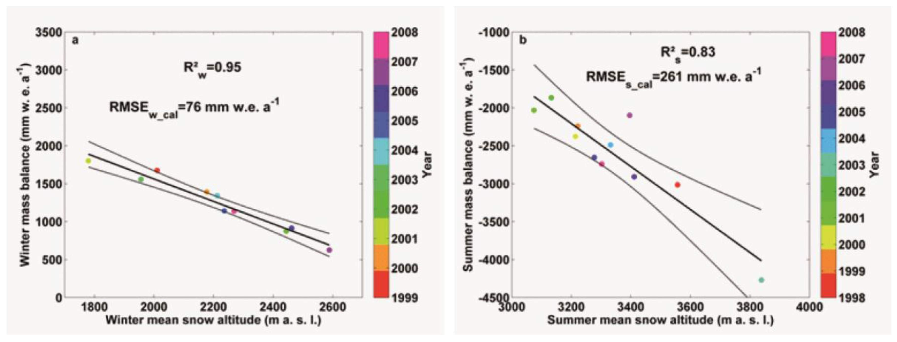
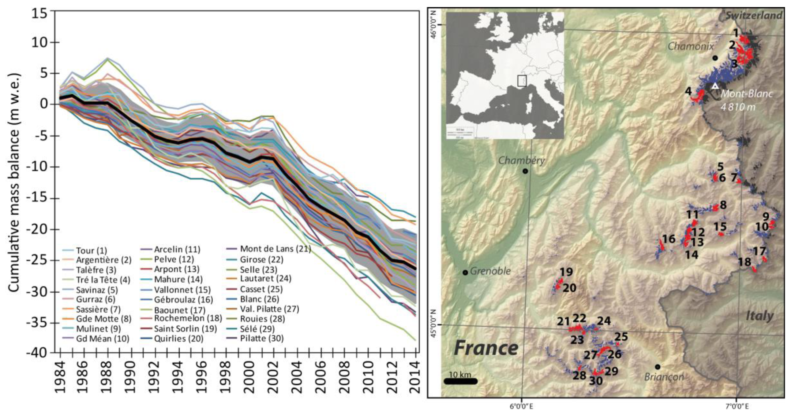
2.1.2. Application of the Method on 30 Glaciers in the French Alps

In a recent study, Rabatel et al. [9] applied the ELA method to quantify the annual SMB of 30 glaciers in the French Alps over the period 1983–2014. For this period, only five glaciers in the French Alps had continuous annual SMB time series quantified from in situ measurements. As a consequence, this study multiplied by six the number of long-term (>30 years) SMB time series in the French Alps. Figure 1 illustrates an example of the snow line identification on the Glacier d’Argentière in the Mont-Blanc Massif from Landsat images.
To quantify the overall glacier mass loss and compute the average annual SMB ( B ¯ in Equation (1)) over the study period, the authors used three DEMs: one dated from 1979 (retrieved from aerial photographs), one from 2003 and one from 2011 retrieved from SPOT-5 stereo images. Regarding the detection of the annual end-of-summer snow line (SLAi in Equations (1) and (2)), the authors used 131 images from different satellites (SPOT 1–5, Landsat 4–8 and ASTER) to cover the 30 glaciers for the 31-year study period. From B ¯ , SLAi and ELAeq, Ba could be quantified for each glacier using Equations (1) and (2). Figure 2 illustrates the cumulative SMB time series. One can note the very good consistency in the inter-annual mass changes between the glaciers related to homogeneous meteorological conditions and inter-annual variability at the regional scale. This result is in good agreement with the homogeneity in inter-annual glacier mass changes quantified from in situ point surface mass balance data at the scale of the European Alps [26] and in other regions of the world [27]. On the other hand, Figure 2 shows that the cumulative mass loss at decadal time scales varied considerably from one glacier to another, and the authors showed that the changes in glacier surface area and length are not representative of changes in mass balance at this decadal time scale. On the other hand, Rabatel et al. [9] emphasized the shift in the temporal trend of glacier mass loss in the early 2000s, with a 3.25-fold increase in the average mass losses by the 30 glaciers between the periods of 1983–2002 and 2003–2014 (−0.47 and −1.52 m w.e. year−1, respectively).
Regarding the ELA method, Rabatel et al. [9] provided evidence for the different sources of uncertainty in the quantified annual glacier-wide SMB coming from each of the variables in Equations (1) and (2) and the one related to the temporal difference between the date of the used satellite image and the end of the hydrological year. The authors concluded that the overall uncertainty in the glacier-wide annual SMB equals ±0.22 m w.e. year−1 on average considering all of the studied glaciers and all of the years (ranging from ±0.19–±0.40 m w.e. year−1 depending on the year and glacier concerned). They showed that the main sources of uncertainty results from: (1) the average annual SMB over the entire period computed by DEM differencing, which depends on the quality of the available DEM (this uncertainty is estimated at ±0.12 m w.e. year−1 in Rabatel et al. [9]); and (2) the temporal difference between the date of the used satellite image and the end of the hydrological year (±0.09 m w.e. year−1 on average, but ranging from 0 to ±0.33 m w.e. year−1 in Rabatel et al. [9]).
Rabatel et al. [9] also considered the impact of using an intermediate DEM when the study period is long (e.g., several decades). Indeed, to quantify the average annual SMB over the entire period by DEM differencing, the mean surface area of the glacier is generally taken as the arithmetic mean of the initial and final areas. This assumes that surface area and SMB trends are linear, which is not necessarily true. Accordingly, the authors concluded that for the study period of several decades with potential periods of glacier mass gain and loss, using an intermediate DEM is recommended to reduce errors related to non-linear changes in surface area.

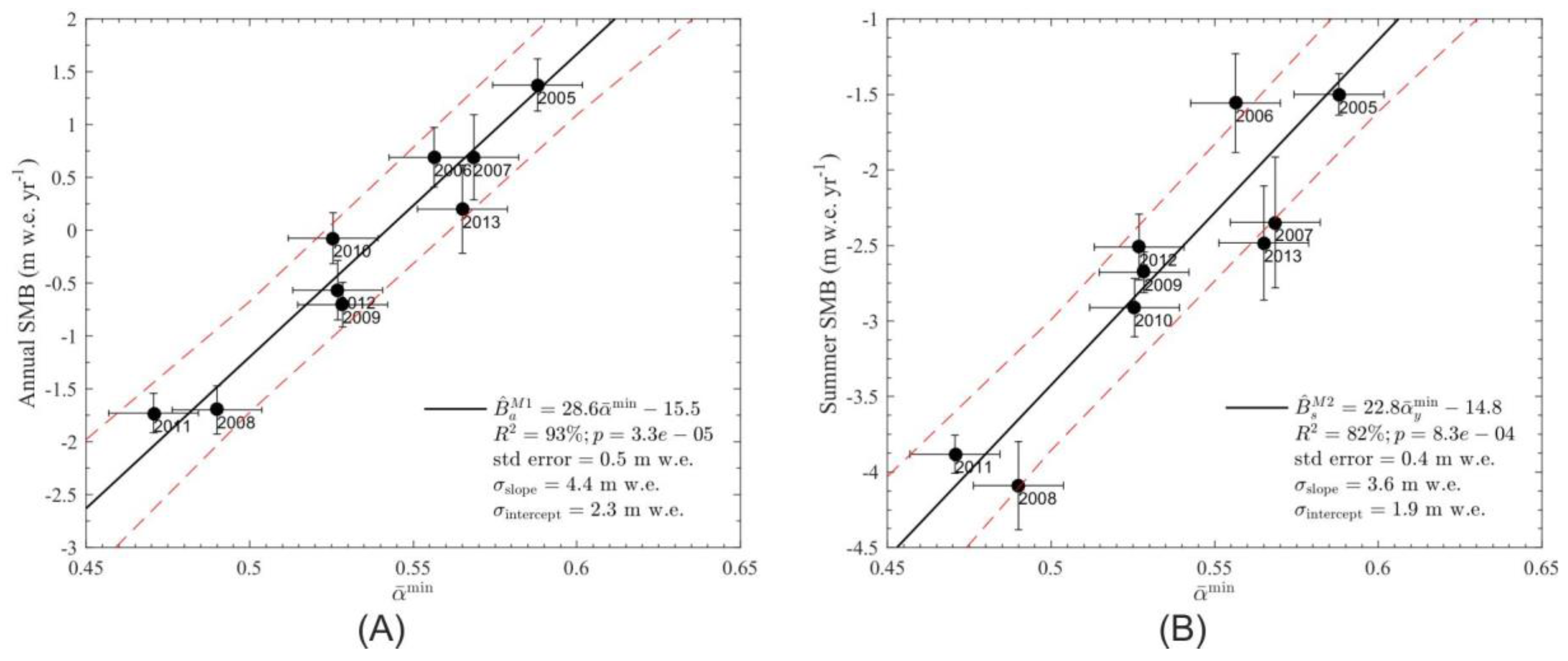
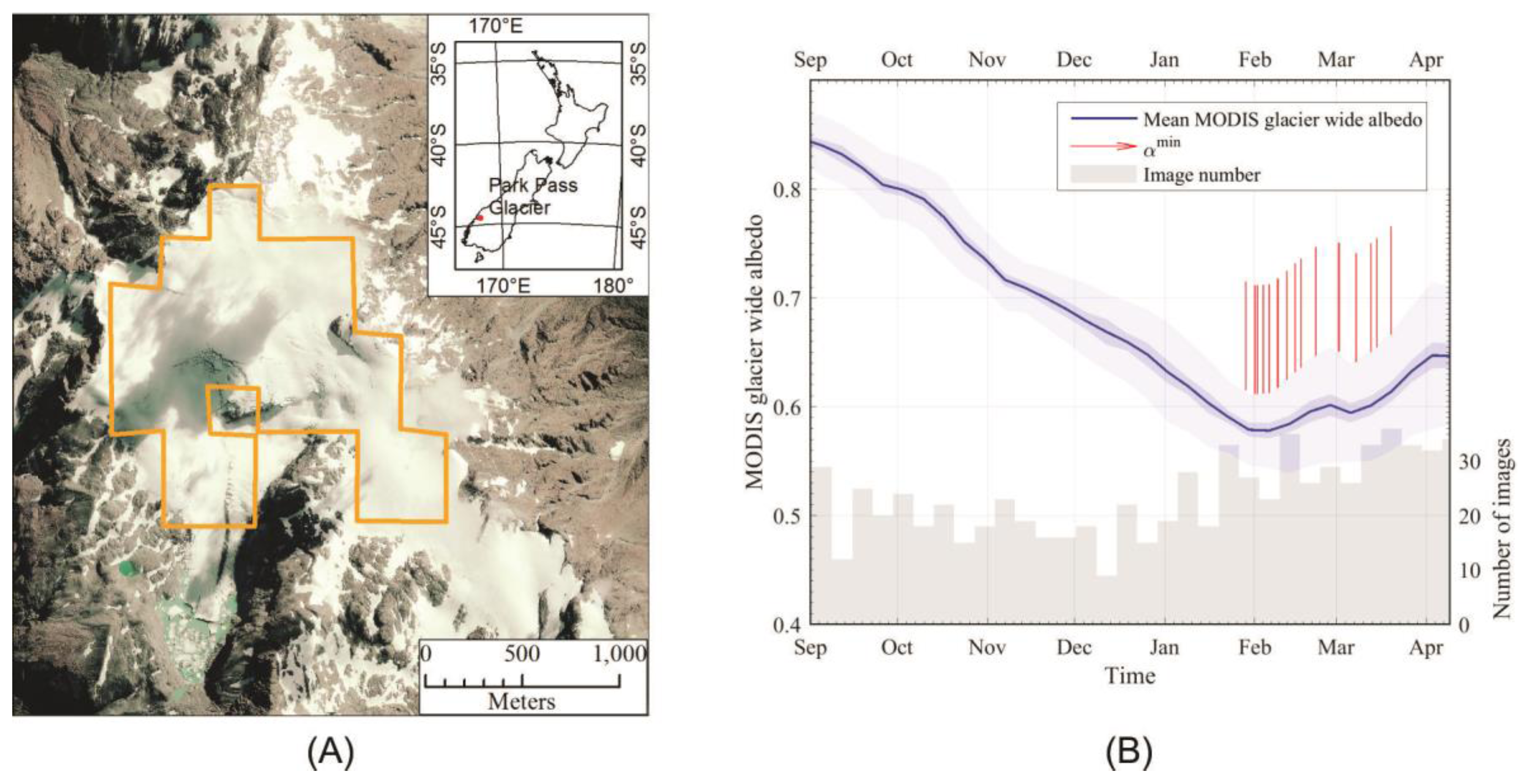
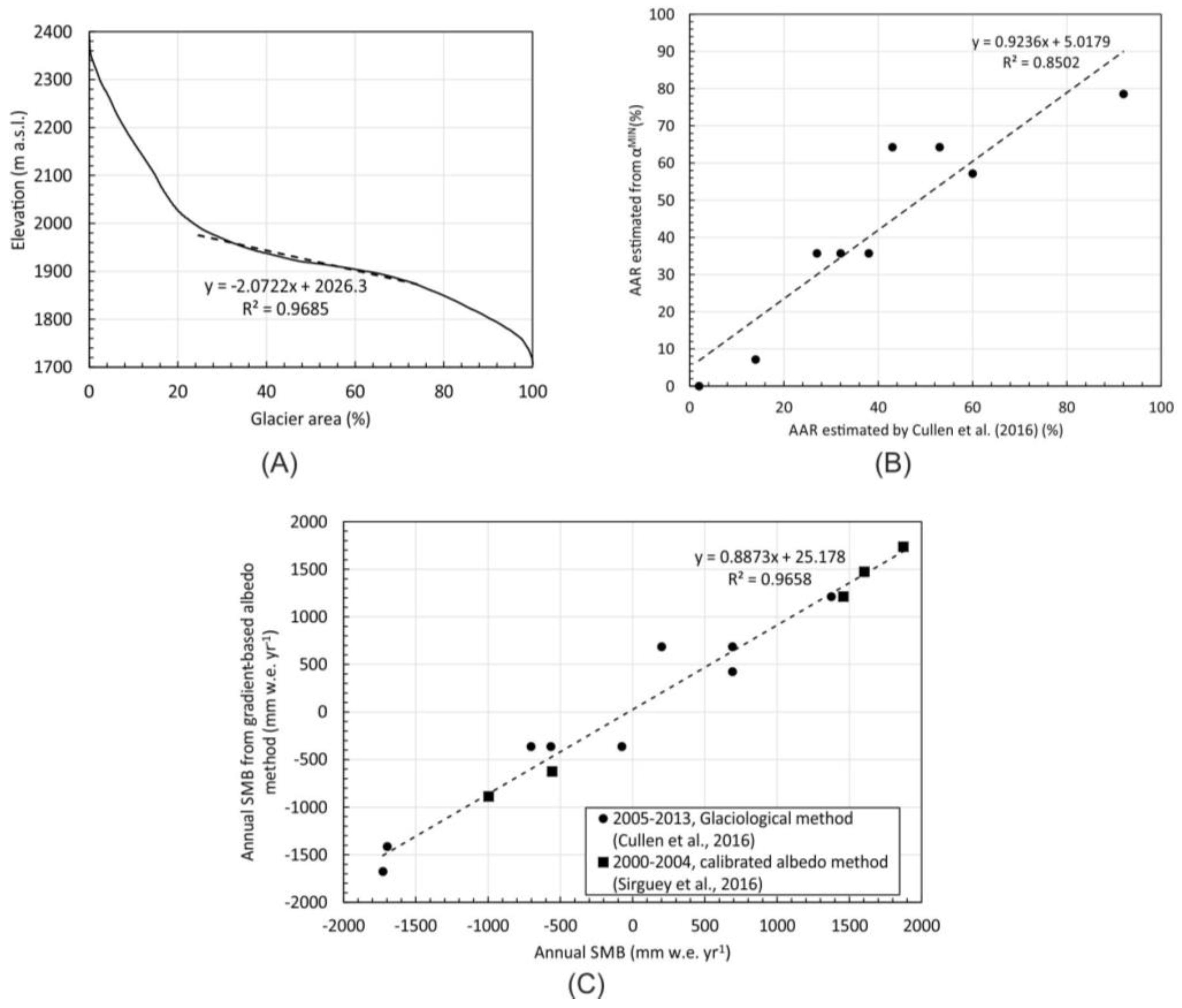
2.2. The Albedo Method

2.2.1. Principles and History of the Method

The albedo, α, of a surface measures the ratio of solar radiation being reflected by this surface. In the case of snow and ice targets, albedo often controls the surface energy budget that in turn governs glacier ablation (e.g., [28,29]). On temperate glaciers, this control accentuates during the ablation season as relatively high reflective snow (α ≈ 0.8) progressively gives way to more absorptive ice surfaces (α ≈ 0.4 or less), concurrently with a significant increase in daily shortwave radiation [30,31]. The rationale behind the albedo method thus stemmed from the capacity of glacier surface albedo to integrate processes of accumulation (e.g., albedo rising with fresh snowfall) and ablation (decrease of albedo as snow transforms and/or the glacier ice is increasingly exposed) combined with its significant physical control on net energy fluxes.
In attempting to estimate the mass balance of Vatnajökull using AVHRR data, pioneers of this approach, De Ruyter De Wildt et al. [32], faced difficulties in resolving the equilibrium-line due to ambiguities in the transition between ice, firn and snow, further complicated by cloudiness. Having converted spectral reflectance to broadband albedo, these authors averaged the albedo over the glacier surface, hereby named glacier-wide albedo, α ¯ . The sum of absorptance (i.e., 1 − α ¯ ) weighted by the extra-terrestrial solar radiation and integrated over a summer was postulated and found to correlate well with the surface mass balance. Greuell and Oerlemans [33] confirmed and refined this approach on a transect in Greenland by using the satellite-derived albedo in an approximation of the energy budget instead of an empirical regression. The method was then applied more widely by Greuell et al. [8] to resolve inter-annual anomalies in SMB of 18 Svalbard glaciers found to be consistent with observations. Nonetheless, Greuell et al. [8] stressed discrepancies between observations and satellite estimates that impair the usefulness of the method when not calibrated by absolute values of SMB.
Dumont et al. [34] revisited this approach by building upon progress in the atmospheric and topographic corrections of optical imagery [35], combined with an improved retrieval method of snow and ice albedo [36]. This allowed time series of glacier surface albedo of mountain glaciers to be derived from MODIS data. Under the simplest assumption that, at the end of the ablation season, a glacier of surface A accounts for a relative share between an accumulation zone of area A a c c , covered by snow with an average albedo of α s n o w , and an ablation zone of area A a b l , exhibiting exposed glacier ice with an average albedo of α i c e , then assuming a linear mixing of the reflectance, the glacier-wide albedo can be obtained as:
α ¯ = α s n o w A a c c + α i c e A a b l A .
Using A A R = A a c c A = 1 A a b l A , it turns out that:
α ¯ = α i c e + A A R ( α s n o w α i c e ) .
In other words, the glacier-wide albedo is a case of linear spectral mixing that directly approaches the AAR with the sensitivity of α ¯ to AAR being controlled by the contrast in albedo between the exposed ice and the snow at the end of the ablation season. Note that this also requires that the albedo of snow and ice at the end of the ablation season remain constant from one year to another.
By leveraging frequent MODIS observations, Dumont et al. [34] used the minimum reached by α ¯ at the end of the ablation season, namely α ¯ min , to capture the AAR. In turn, and consistently with studies showing AAR to be a good predictor of SMB (e.g., [14,37,38]), Dumont et al. [34] showed that α ¯ min could be used as a surrogate for the annual SMB on Saint-Sorlin glacier (French Alps) using a simple linear model, namely:
B a = s α ¯ min + o ,
where s and o are the slope and offset of the linear regression, respectively.
Using a similar approach, Wang et al. [39] also obtained significant correlations between α ¯ at the end of summer and annual SMB on two glaciers in western China. Brun et al. [40] further tested the method on Chhota Shigri (India) and Mera (Nepal) glaciers in Himalaya allowing annual SMB series to be reconstructed over the period of MODIS observations. The correlation between α ¯ min and B a on Mera Glacier was found to be less robust because of persistent cloud cover and snow accumulation during the monsoon season that prevented the seasonal variations of α ¯ to be fully resolved despite near-daily imaging with MODIS. As a summer accumulation type glacier, Mera Glacier also exhibited a relatively narrow range of α ¯ min that contributed to a weaker linear model. A linear correlation between surface mass balance and albedo over Greenland’s terrestrial ice was also shown by Colgan et al. [41] and used to estimate monthly surface mass balance. Finally, Sirguey et al. [42] successfully applied the albedo method on Brewster Glacier in New Zealand, allowing the relatively short record of in situ measurements to be reconstructed over 37 years.

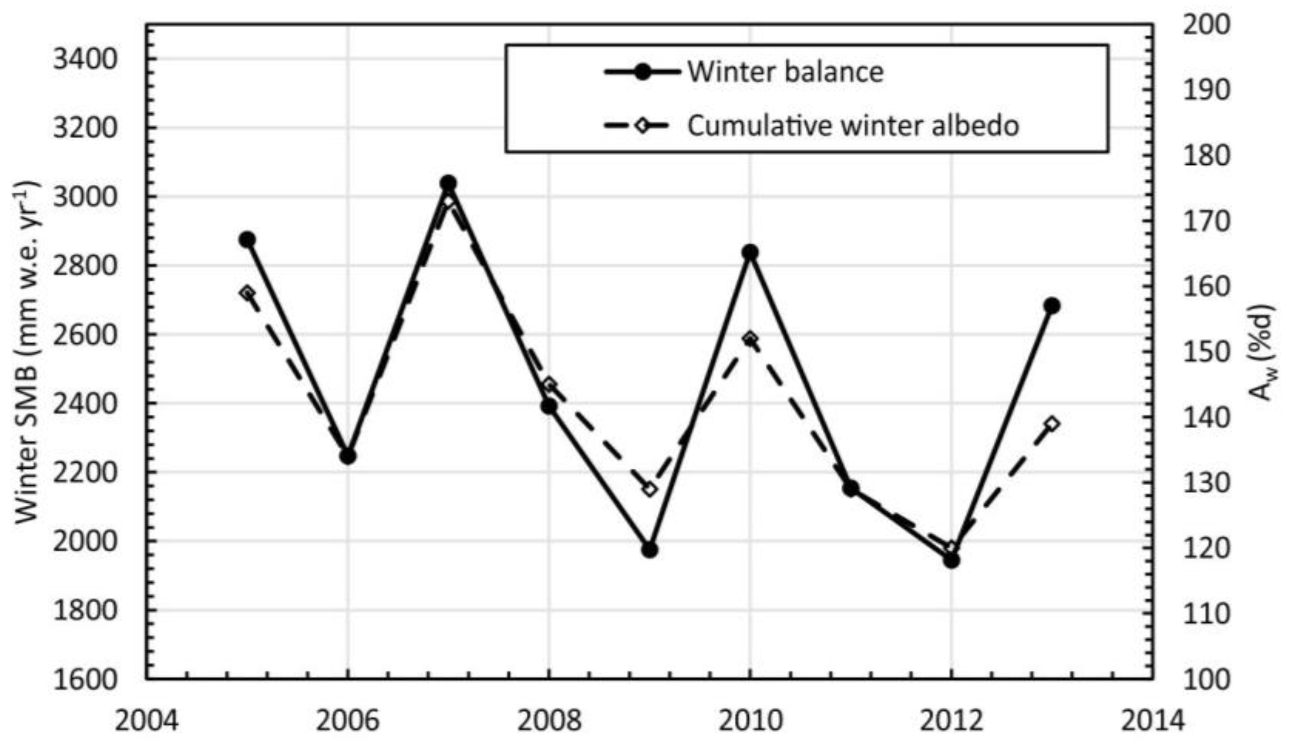
2.2.2. Application of the Albedo Method on New Zealand Southern Alps Glaciers

Only a few direct SMB studies have been made in the Southern Alps of New Zealand, bringing relatively short-term observations [43]. In lieu of direct glaciological monitoring, annual aerial surveys have been conducted since 1977. Oblique photographs captured at the end of the austral summer are used to document the position of the snow line (end-of-summer snow line, corresponding to the SLAi in the previously-described ELA method) on 50 “index” glaciers, which sample several transects along and across the alpine range. The photographic record supports estimates of SLAi as the annual ELA of glaciers, whose inter-annual variability is used as a surrogate to glacier mass-balance changes [22]. Cullen et al. [38] recently consolidated the longest in situ record of a glacier SMB in New Zealand, namely Brewster Glacier. The study documented the relationship between AAR, ELA and SMB and supported the validity of linear approximations within a range of variations of ELA or AAR. Sirguey et al. [42] confirmed the potential of the albedo method in New Zealand with α ¯ min found to be a suitable proxy to estimate both the annual and summer SMB (Figure 3). It enabled the SMB series of Brewster Glacier to be reconstructed over the period of MODIS acquisition and confirmed the potential of frequent monitoring of glacier surface properties as a method capable of sustained systematic observations of the glacier SMB signal.
Among the four index glaciers of more than 2 km2 monitored in New Zealand, variations of MODIS glacier-wide albedo were obtained for Park Pass Glacier from which yearly values of α ¯ min could be obtained (Figure 4). Figure 4B confirms the conclusion by Sirguey et al. [42] that α ¯ min is expected to be reached in early February. α ¯ min values for each year on Park Pass (2000–2015) and Brewster (2000–2013) glaciers are plotted against the corresponding S L A i from the snow line aerial survey program in Figure 5. In the two cases, α ¯ min captures nearly 90% of the variance of S L A i , thus stressing its potential to supplement the EOSS program, for example to generate SMB signals of New Zealand glaciers larger than those currently included in the aerial surveys.
Therefore, the albedo method can capture a SMB signal comparatively relevant to that of the snow line aerial survey program (analogue to the ELA method). Moreover, the albedo method has the advantage of being available from satellite remote sensing and a potential of generalization to monitor an entire glacierized region with less logistical burden. However, the conversion of α ¯ min to SMB values has, so far, been approached only via calibration with in situ data. It is possible to propose a development of the albedo method inspired from the ELA method to quantify the SMB readily from α ¯ min , namely a gradient-based albedo method. First, we note that the SMB-elevation gradient b / z , used by Rabatel et al. [13] can be converted into an SMB-area gradient b / A A R , using the hypsometric curve of a glacier using:
b A A R = b z × z A A R .
For example, on Brewster Glacier, Cullen et al. [38] found that b z = 1.75 m w.e. 100 m−1 across E L A e q . From the hypsometric curve shown in Figure 6A, z A A R is found to be ca. −2.1 m %−1. The value of b A A R can be estimated as −36.7 mm w.e. %−1. From Cullen et al. [38], the average annual SMB over the period of 2005–2013 is estimated to B ¯ = −0.201 m w.e. year−1 (note that the latter could be obtained from the geodetic method that uses DEM differencing). Using α ¯ min values derived by Sirguey et al. [42] and assuming α s n o w = 0.62 (old snow) and α i c e = 0.48 similar to the observations made by Cullen and Conway [31], Equation (4) yields estimates A A ^ R i that match the values obtained from re-analysis of in situ measurements (Figure 6B). With regards to the ELA method, the AAR of a glacier in equilibrium can be estimated by:
A A R e q = 1 n A A ^ R i + B ¯ b A A R .
Using the values above, we find A A R e q = 47% for Brewster Glacier, which is close to the estimate based on the hypsometric curve (46%) reported Cullen et al. [38]. Finally, yearly values of surface mass balance B a can be estimated by:
B a = ( A A R e q A A ^ R i ) b A A R .
Figure 6C illustrates the good agreement between SMB values of Brewster Glacier derived by the gradient-based albedo method and those initially obtained via direct regression with in situ measurements. Although this example only serves as a proof of concept, it shows that the approach of the ELA method can be generalized to the albedo method successfully. Similar to Rabatel et al. [13] and Chinn et al. [43] who postulated that b z could be extrapolated to glacier (sub-)regions to apply the ELA method, a similar assumption could be made along with a specific glacier hypsometric curve to extrapolate the gradient-based albedo method to glaciers with no in situ measurements.
Finally, the albedo method proved to support more than the annual balance only. Sirguey et al. [42] hypothesizes that, in addition to B a , the temporal variation of α ¯ could also support a signal related to summer and winter mass balance B s and B w , respectively. α ¯ min was found to correlate well with B s , which is consistent with glaciers whereby the variability of annual SMB is predominantly controlled by the variability of summer SMB [38,44]. Furthermore, Sirguey et al. [42] proposed the cumulative winter albedo A w , namely the integration of α ¯ over the accumulation season when α ¯ exceeds a threshold α t h large enough to capture conditions favourable to winter balance:
A w = w i n t e r { α ¯ ( t ) , α ¯ ( t ) α t h 0 , o / w d t .
A significant correlation was found between winter SMB and A w that allowed B w to be estimated using a linear model. The concurrent evolution between A w and B w illustrated in Figure 7 supports that a signal of winter balance can be captured by monitoring variables of the glacier surface that integrate events that are favourable to winter accumulation. This result resonates with the following section of the paper whereby the inter-annual variability of the snow cover around glaciers during summer and winter is also shown to explain the variability of the seasonal SMB.

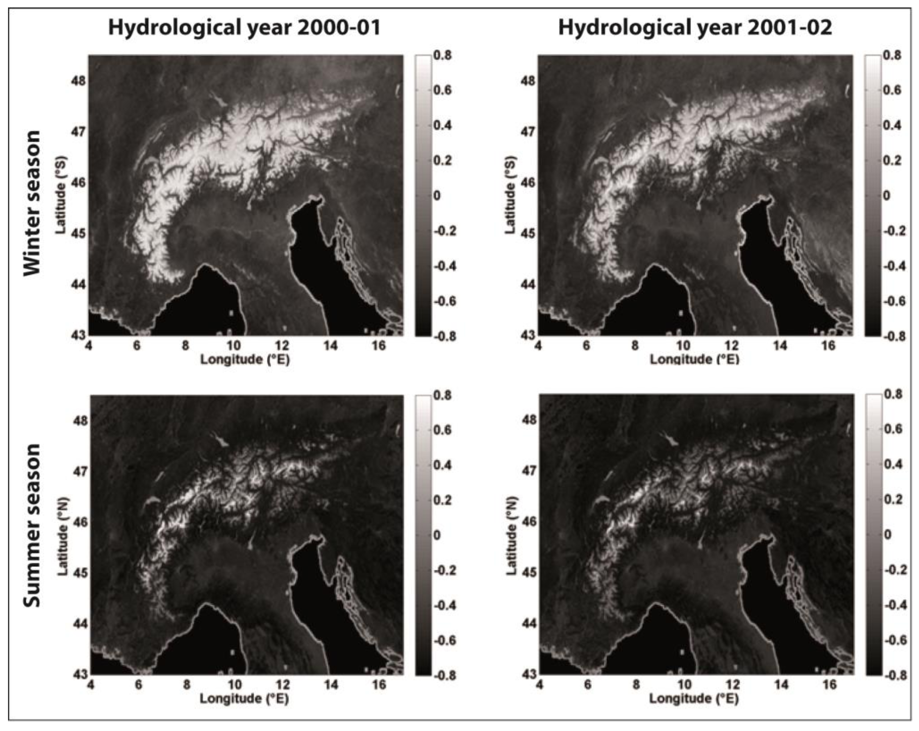
2.3. The Snow-Map Method

2.3.1. Principles and History of the Method

This method is based on regional snow maps from daily optical satellite images (e.g., the daily 1-km resolution SPOT/VGT and PROBA-V images) to quantify glacier seasonal SMB. The method hypothesizes that the seasonal mean snow altitude around a glacier is a proxy for the seasonal glacier SMB.
The first step consists of calculating the normalized difference snow index (NDSI) from the satellite images to produce daily snow maps for the winter and summer seasons of the study area during the period covered by the satellite data (e.g., 1998–2014 for SPOT/VGT, 1-km pixel resolution). The NDSI was introduced by Crane and Anderson [45] and Dozier [46] for the Landsat sensor. The index has since been widely used with different sensors (e.g., [47,48,49]). The NDSI value is proportional to the snow cover fraction inside the pixel and allows an efficient monitoring of the spatial and temporal snow cover variations [50]. In Drolon et al. [51], an NDSI adapted to the SPOT/VGT sensor was proposed, inspired by Chaponnière et al. [50], computed from the mean of the red (B0) and blue (B2) channels and from the SWIR band:
N D S I = ( B 0 + B 2 2 S W I R ) / ( B 0 + B 2 2 + S W I R ) .
A cloud mask is applied in order to flag cloudy pixels and to avoid overestimating the snow coverage. A temporal interpolation is then computed for the “cloudy” pixels. Maps of winter/summer NDSI are produced by averaging all NDSI syntheses (10-day syntheses for SPOT/VGT images) included between 1 October and 30 April for each winter and between 1 May and 30 September for each summer (Figure 8).
Then, the seasonal snow maps are overlaid on a DEM (e.g., SRTM30) to derive the seasonal altitudinal distribution of NDSI in an optimized area surrounding each studied glacier called the windows of snow monitoring (WOSM). The inter-annual variability of the altitudinal distribution of NDSI within the WOSM surrounding the glacier is thus obtained for the studied period (16 years for SPOT/VGT; Figure 9). From the intersection between an optimized NDSI value (specific to each glacier) and each curve of the NDSI seasonal altitudinal distribution, a “mean regional” altitude of snow (Z) can be deduced for summers and winters of the study period.
Finally, a linear regression between the mean regional snow altitudes Z and the seasonal SMB is quantified (Figure 10). This linear regression allows the estimation of the glacier seasonal SMB, as a function of Z inferred from satellite images (see Equation (11), generalized for both seasons):
B w / s _ VGT = w / s Z w / s + β w / s .
Bw/s_VGT is the winter/summer SMB estimated for the year y (in m w.e. year−1); Zw/s is the winter/summer “mean regional” altitude of snow (in m); the slope coefficient αw/s (in mm w.e. year−1 m−1) represents the sensitivity of a glacier winter/summer SMB towards Zw/s; and βw/s is the winter/summer intercept term (in mm w.e. year−1).
For each glacier, different sizes of WOSM and different seasonal NDSI values can be applied. Both WOSM and NDSI values are adjusted in order to minimize the RMSEw/s_cal between the observed and simulated seasonal SMB. The cost function f optimizing the RMSEw/s_cal for a glacier is thus:
f ( N D S I * , W O S M * , α w / s , β w / s ) = min ( y = 1 N ( B w / s _ VGT   y B w / s _ ref   y ) 2 N ) .
NDSI* and WOSM* are respectively the NDSI value and the WOSM side length minimizing the RMSEw/s_cal. Allowing the adjustment of both the NDSI value and the WOSM size is a means to select an optimized quantity of snow-covered pixels (where snow dynamics occurs) that are less affected by artefacts like residual clouds, aerosols and/or directional effects.
To apply the snow-map method, the following are needed:
  • Several optical satellite images for each season of the studied period, covering the region of interest (ROI).
  • One DEM of the ROI acquired during the studied period.
  • Observed seasonal SMB available over the studied period covered by the satellite (or for sub-period of the study period).

2.3.2. Application of the Method on 55 Glaciers in the European Alps

This method has been applied for 55 glaciers in the European Alps with SPOT/VGT images by Drolon et al. [51]. Promising linear relationships between the regional mean snow altitude and observed seasonal SMB have been found over the calibration period 1998/1999–2008. The explained variance in winter is statistically significant for all glaciers (R2 = 0.84 on average), and the average RMSE (161 mm w.e. year−1) is below the usual error Eobs associated with glaciological SMB measurements (typically included between ±200 and 400 mm w.e. year−1).
For the summer period, the explained variance is lower, although still statistically significant (R2 = 0.73 on average) with the averaged RMSE (318 mm w.e. year−1) still in the range of Eobs. An individual cross-validation of the 55 linear regressions allowed validating the temporal stability and the robustness of 95% of the relationships in winter and of around 60% of the relationships in summer.
Beside the individual calculation of each glacier SMB presented in Drolon et al. [51], we illustrate here a synthetic result through the mean reconstructed and observed MB time series averaged for the 55 studied glaciers (Figure 11). In winter (Figure 11a), <Bw_VGT> is generally in close agreement with <Bw_obs>. The highest absolute mean SMB errors |MBEw_cal| (i.e., the mean difference between Bw_VGT and Bw_obs for all the glaciers) (175 mm w.e. year−1 in 2005) is smaller than Eobs and than the standard deviation of the observed winter SMB of all glaciers σw_obs (615 mm w.e. year−1 in 2005). Moreover, the two contrasted 2001 and 2002 winter are well-captured by the model. In summer (Figure 11b), <Bs_VGT> accurately reproduces <Bs_obs>, and the large inter-annual variations are well captured. The lowest SMB values are observed in 2003 reflecting the exceptional summer heat wave of 2003. The summer absolute mean SMB error |MBEs_cal| is the highest in 2007 (448 mm w.e. year−1) and 2003 (356 mm w.e. year−1), but remains still inferior to the standard deviation of the observations (594 and 559 mm w.e. year−1 for 2007 and 2003, respectively).
The relationships calibrated over the period 1998–2008 have then been applied to the evaluation period 2009–2014. Seasonal surface mass balance in situ data on the 55 studied glaciers across the European Alps show that the method is able to retrieve the winter SMB without bias and with an acceptable mean error (417 mm w.e. year−1) over 2009–2014. In summer, the mean error of SMB estimation over 2009–2013 is higher than in winter (561 mm w.e. year−1) and slightly above Eobs.
The possibility of a generic and transferable relationship between Z and seasonal SMB has also been investigated to apply the methodology on glaciers where no in situ SMB data are available. For each season, a generic model has been built by averaging the αw/s and βw/s coefficients obtained from the cross-validated relationships. Additionally, the NDSI values and WOSM sizes are adjusted in order to minimize the mean RMSE for the glaciers used for validation. Then, the ability of the resulting generic model to retrieve the 55 glaciers’ seasonal SMB was assessed. In winter, the generic model showed significant results over the entire study period 1998–2014 (mean RMSE of 411 mm w.e. year−1 as regards Eobs). However, errors produced by the summer generic model are high (714 mm w.e. year−1). The high inter-annual variability of the alpine glaciers’ summer SMB is not well captured by the generic model.

3. Discussion

3.1. Limits of the Methods

3.1.1. Cloud Cover

The three methods based on optical satellite imagery presented here are subject to the limitation of cloud cover. Regarding the ELA method, this issue becomes progressively less important with the multiplication of satellites acquiring images at a decametric spatial resolution (e.g., Landsat, ASTER, SPOT, Sentinel-2) and in some cases with a short revisiting time period (e.g., five days for Sentinel-2). In addition, Rabatel et al. [9] have shown that using images recorded within one month before the end of the hydrological year (i.e., between mid-August and late September for the Northern Hemisphere mid-latitudes) generates accurate annual SMB values because the elevation changes of the snow line at the end of the summer are limited. Another alternative could be the use of radar data, which showed promising results for the identification of the end-of-summer snow line [52,53].
The albedo method is also affected by cloud obstruction, although it leverages more frequent imagery at coarser resolution to increase the chances of repeated clear observations spanning the seasonal albedo cycle. For example, due to the persistent cloud cover in New Zealand, nearly 70% of observations are affected by clouds even with near-daily imagery. However, there are still enough good observations sufficiently scattered in time to resolve the albedo cycle. As the method relies on a cloud detection algorithm and due to the difficulties of achieving perfect discrimination between clouds and snow using optical imagery, the albedo method also suffers from omission and commission errors in the cloud detection algorithms. This can however be mitigated via the statistical filtering of time series. Resolving the albedo cycle can become particularly difficult for areas with even more persistent clouds, such as Nepal during the monsoon [40].
Regarding the snow-map method, the effect of pixels contaminated by undetected clouds (e.g., low-altitude clouds located in the valleys) can partly explain the reduced performance for summer. The error in a pixel NDSI value caused by a cloud is smaller for a snow-covered pixel than for a snow-free pixel. As there is less snow in summer than in winter, undetected clouds may impact NDSI and snow detection more in summer.

3.1.2. Glacier Size and Elevation

Regarding the ELA method, the main limiting factor for its application is related to the uppermost elevation reached by the glacier. Indeed, the uppermost elevation must be high enough to allow preserving an accumulation zone at the end of the ablation season. The albedo method leverages high frequency acquisitions to resolve the albedo cycle with sufficient details to retrieve minimums representative of the glacier surface condition at the end of the summer. In remote sensing, this typically involves imagery obtained at coarser spatial resolution. For example, the application presented here has relied on near-daily imaging from MODIS with albedo mapped at 250-m spatial resolution. This nominal footprint is comprised of the panoramic distortion of the across track scanner with about a third of observations acquired under a view angle greater than 45°. In effect, the relatively large pixels favour spectral mixtures with nearby terrain that hinder the quality of the albedo signal [42]. Furthermore, the area from which the glacier-wide albedo is calculated needs to account for pixels in both the ablation and accumulation areas to capture contrast and statistically reduce the noise inherent to the albedo retrieval method via averaging. It has so far been applied only to glaciers of an area greater than 2 km2 captured typically by more than 20 MODIS pixels chosen inside the glacier outlines to minimize spectral mixtures. Glaciers on and/or surrounded by steep topography can also be exposed to severe shadowing that can compromise the albedo retrieval. This happens typically during winter months when relying on morning MODIS/Terra acquisition. Early afternoon imagery from MODIS/Aqua could be used to mitigate this limitation.
For the snow-map method, the uppermost elevation reached by a glacier or the minimum size of a glacier does not constitute an a priori limit of applicability. However, in some rare cases, if the regional snow line rises above mountains, the snow-map method suffers from same issue as the ELA method and does not allow the estimation of the seasonal SMB (after the calibration period). In those particular cases, the NDSI value optimizing the linear relationships between Z and SMB over the calibration period does not intersect the NDSI altitudinal distribution curves (the curves are below the NDSI value). Thus, no SMB can be retrieved, except if the WOSM size is increased (but at the cost of degrading the regression quality). Moreover, the snow-map method does not seem to perform well for large glaciers (e.g., Aletsch Glacier in the case of the application in the European Alps; see [51]), whose ablation area reaches relatively low elevation. Glacier snout can thus remain snow-free for a considerable part of the period used for winter SMB estimate (October–April). Winter SMB data for those glaciers thus include both accumulation and melting, whereas the snow-map method for winter is optimized to represent snow accumulation.

3.1.3. Debris-Covered Glaciers

None of the methods presented in this review has been applied to debris-covered glaciers. It is noteworthy that among the glaciers with long-term in situ monitoring of their surface mass balance that are used to calibrate/validate the remote-sensing methods, the large majority are free of debris, or the debris-covered parts are negligible in comparison with the total surface area of the glaciers. Regarding the ELA method, it is assumed that the glacier-wide mass balance is similar to the surface mass balance obtained in the vicinity of the ELAeq. Rabatel et al. [9] underlined that this assumption is reasonable because the mass balances obtained with the ELA method are normalized by the glacier-wide SMB of the entire study period, using satellite DEM differencing. In the case of heavily debris-covered glaciers, this assumption deserves to be verified. Indeed, ablation processes on the debris-covered areas differ from the debris-free areas and can strongly influence the glacier-wide SMB (e.g., [54]). Studying a small debris-covered glacier in the Everest region, Vincent et al. [55] indicated that, for this particular glacier, the insulating effect of the debris cover has a larger effect on the total mass loss than the enhanced ice ablation due to supraglacial ponds and exposed ice cliffs.
The calibration of the albedo method has not yet been attempted on glaciers with extensive debris cover, but does prove successful when the area covered by debris is small [40]. As the relative share of the debris-covered area increases, a disconnection between SMB of the debris-free area and the glacier-wide SMB may compromise the relationship between AAR and surface mass balance and, in turn, the albedo method. Nonetheless, the suggested development of the gradient-based albedo method will benefit from the same assumption and limitation of the ELA method as it will take similar advantage of the average glacier-wide SMB.
Regarding the snow-map method, it is based on the variability of the seasonal regional mean snow altitude to retrieve the SMB. For glaciers with extensive debris cover, the SMB is controlled by other processes than the snow accumulation/ablation. Hence, the snow-map method may be less relevant to retrieve seasonal SMB of debris-covered glaciers.

3.1.4. Polar and Monsoon-Regime Glaciers

The presented methods have been applied on temperate glaciers of the mid-latitudes and also on glaciers located within the outer-tropics of the Andes in the case of the ELA method [21].
The ELA method requires that the elevation of the snow line at the end of the hydrological year must be representative of the ELA. In the case of polar glaciers where the formation of superimposed ice can represent a significant part of the accumulation, such a requirement is not verified, and the ELA method cannot be applied. It is also the case for equatorial glaciers where accumulation at the glacier surface is almost constant all year long (e.g., [56]) or glaciers located in mountain ranges where a monsoon regime co-exists with a winter precipitation regime.
The albedo method initially relies on a linear relationship between AAR and SMB, which has been shown to be a common case [37]. It leverages a well-defined seasonal albedo-cycle whereby the minimum albedo is reached at the end of the ablation season. Glaciers with less seasonal contrast in surface albedo, due for example to a mixed ablation/accumulation regime, such as during monsoon, may complicate this relationship. Nevertheless, Brun et al. [40] found that minimum glacier-wide albedo could still capture valuable variance of the SMB on a monsoon influenced glacier (Mera) in the Himalayas.
The snow-map method hypothesizes that the seasonal mean snow altitude around a glacier is a proxy of the glacier seasonal SMB. It works well for temperate glaciers whose winter/summer SMB is mainly controlled by snow accumulation/melting. The method relies on the variability of the seasonal snow cover, easily detected when there is a seasonal partitioning of the snow accumulation and ablation. The snow-map method will therefore be less efficient for equatorial or monsoon-regime glaciers.

3.1.5. Spatial Distribution of Surface Mass Balance

The presented methods increase the number of monitored glaciers for their glacier-wide annual to seasonal surface mass balances, but none of the methods allows retrieving the spatial distribution of surface mass balance.
In the case of the albedo method, further work is needed in this area and to link the albedo value (annual minimum or integrated albedo value over the winter or summer season) of each pixel to its annual or seasonal surface mass balance. However, the 250-m spatial resolution of the currently-used MODIS images might be a limitation because with such a large pixel size, the albedo value of the pixel could hardly be related to the SMB at one point (i.e., a stake) within this pixel. In the case of relatively small mountain glaciers, individual pixels remain potentially affected by varying pixel footprints and spectral mixtures that are compounded by the uncertainties inherent to the topographic and atmospheric corrections and albedo retrieval algorithm. However, the Sentinel-2 images, available at a 10-m spatial resolution every five days, open interesting perspectives to resolve albedo cycles from smaller distinct areas of a glacier from which local SMB information may be obtained.

3.2. Future Challenges

3.2.1. Automating the Data Processing

Regarding the ELA method, the next step will be automating the method in order to apply it globally or at least for glaciers where the end-of summer snow line can be considered as a proxy of the ELA. Such a global application still needs to tackle some problems such as automating the detection of the end-of-summer snow line and the computation of its elevation. Different spectral band combinations or band ratios can be tested [21], associated with cloud and shadows masks. Another important issue for the long-term application of the ELA method is to find DEMs of sufficient accuracy to compute the geodetic balance from the 1970s or 1980s, which for some mountain ranges, might not be easy.
Regarding the albedo method, by relying on the systematic processing of frequent image acquisitions, the method requires automating. This has been achieved via the MODImLab MATLAB toolbox whereby the downloading and processing of thousands of MODIS images can be efficiently batched. MODImLab also provides algorithms to compute isotropic and anisotropic albedos [34] for every MODIS pixels, allowing end-users to easily obtain albedo maps.
Regarding the snow-map method, the data processing is partly automated. Indeed, a chain of MATLAB routines allows processing the downloaded SPOT/VGT images and the DEM in order to estimate the seasonal SMB.

3.2.2. Use of Other Images

Regarding the ELA method, the application presented here used high-resolution satellite images (i.e., SPOT, Landsat, ASTER). However, as mentioned earlier, the method of mapping the end-of-summer snow line can be based on different sources, from very high resolution aerial photographs (e.g., [15,16] and, more recently, [22]) to medium resolution satellite images like MODIS data (e.g., [24,57,58]) when the studied ice bodies are wide (i.e., hundreds to thousands of km2).
Adaptation of the albedo method to other sensors (currently only MODIS) is also needed. There is a good prospect for sustainable observations of glacier surface by upcoming satellite programs such as Sentinel-3 and JPSS constellations, both embarking instruments capable of providing high temporal revisit frequency at the regional scale similar to MODIS. Image processing currently done for MODIS to retrieve horizontal equivalent reflectances and retrieve surface albedo of snow and ice needs to be adapted to the new spectral resolution. Further adaptation of the albedo retrieval to Landsat-8 and Sentinel-2 data is also needed to research the potential of resolving the spatial distribution of SMB, as well as mitigating the spectral mixture affecting albedo retrieval from currently coarse pixels. The combination of observations from Landsat-8 and Sentinel-2 may achieve sufficient redundancy to resolve the albedo cycle, albeit at a higher cost in computing resources.
Applying the snow-map method with images from other optical sensors is possible as far as the temporal resolution of image acquisition makes possible the calculation of seasonal snow maps. Such an exercise has already been initiated with observations from the PROBA-V satellite, launched in May 2013 in order to continue the SPOT/VGT mission (which ended in May 2014). Note that a similar exercise is still needed with MODIS and Sentinel-3 data. Regarding PROBA-V, an inter-calibration of the NDSI computed from the PROBA-V 1-km resolution images and from the SPOT/VGT images has been achieved by Drolon [59] over the acquisition overlap period of the two sensors (October 2013–May 2014). Consistency has been found between winter SMB estimations from the two sensors, in 2013–2014. A “near real-time” seasonal SMB monitoring is thus conceivable with PROBA-V or any other daily resolution optical imagery for a large sample of Alpine glaciers, if an inter-calibration of the satellite data can be achieved. Low resolution optical satellite images are available two to three days after the acquisition dates, implying that seasonal snow cover and seasonal SMB could be estimated a few weeks after the end of each season.
PROBA-V also provides images at 300 m and 100 m spatial resolution. A study is underway to assess the impact of the PROBA-V image resolution on the accuracy of the seasonal SMB estimated with the snow-map method. In fact, the 100-m resolution PROBA-V images could improve the seasonal SMB estimates, especially the summer ones. The summer mean regional snow altitude detected with the PROBA-V 100-m images could be closer to the snow line notion. The snow-map method applied for the summer period could certainly also take advantage of higher resolution images (like Landsat-8 and/or Sentinel-2) that would enable the inter-annual monitoring of residual small snow-covered surfaces (snow patches). More research is needed in this area.

3.2.3. Generalization of the Calibrated Methods

The methods based on the albedo and regional seasonal snow maps are currently used on glaciers where in situ SMB data are available for calibration. However, in both cases, a generalization can be made to apply these methods on glaciers where no SMB data are available, as in the case of the ELA method.
Section 2.2.2 proposed a way forward to generalize the albedo method to avoid reliance on current calibration with in situ data. It is suggested that such an approach could mimic the ELA method by using long-term geodetic estimates of average glacier-wide SMB and the use of the mass-balance gradient. An SMB-area gradient can be made as the analogue to the SMB-elevation gradient via the use of glacier morphometry. The regionalization of such a gradient could then allow estimates of SMB for unmonitored glaciers.
Regarding the snow-map method, a generic relationship showed good performance for winter SMB, even on non-monitored glaciers (without calibrated relationships established between Z and SMB). Indeed, for a dataset of 15 glaciers of the Alps, the winter generic relationship showed a satisfying RMSE (490 mm w.e. year−1). The winter generic model can thus be applied at the scale of the European Alps to sufficiently estimate winter SMB of glaciers for which no in situ data are available. The application of this generic model to other mountain ranges requires further developments.

4. Conclusions

We presented a review of three existing methodologies based on optical satellite images to quantify the glacier-wide seasonal to annual surface mass balances. These methods show promising results to considerably increase the number of time series of surface mass balance; a glacier variable necessary to better understand the relationship between climate and glacier changes, as well as the contribution of glaciers to the hydrological regime of glacierized catchments. It is worth noting that the best method will vary by region, depending on, for example, cloudiness, glacier size or maximum elevation.
Even if the albedo method and the snow-map method have currently been applied on glaciers where in situ SMB data were available for calibration purposes, both methods can be generalized to be applied on unmonitored glaciers as in the case of the ELA method.
Regarding the seasonal SMB, it is noteworthy that the albedo method performs better for the summer SMB, which can be efficiently quantified from the minimum average albedo value of the glacier surface area, or the integration of this value over the entire summer period. On the other hand, the snow-map method shows better performance for the quantification of the winter SMB because the method is based on the variations of the seasonal altitude of the snow cover distribution, which are significantly representative of the winter SMB; whereas in summer, the variations of the seasonal altitude of the snow cover distribution are lower and limited to representing the high year-to-year variations of summer SMB.
As a consequence, a further exercise could consist of applying the three methods simultaneously to the same glaciers to take advantage of the better performance of each method. In that sense, the winter SMB could be quantified from the winter snow maps, the summer SMB quantified from the albedo method, and then, a cross-validation between the annual SMB quantified from the ELA method and from the sum of the two seasonal components could be done.
Finally, it is worth noting that the three methods were developed, calibrated and validated on temperate glaciers of the mid-latitudes (and outer tropics) with no or limited debris coverage. We suggest that for polar glaciers or glaciers in the equatorial and monsoon-regime regions, these methodologies might not be efficient, and the methods need to be adapted or alternative methods need to be found.

Acknowledgments

The authors are grateful to the spatial agencies CNES, ESA, NASA and VITO, for providing free access (or with a reduced cost) to the satellites images. The French Service National d’Observation GLACIOCLIM (http://glacioclim.osug.fr/) and the World Glacier Monitoring Service (http://wgms.ch/) are acknowledged for the collection and distribution of in situ glaciological data used to calibrate/validate the remote-sensing based method. Authors from the University of Grenoble Alpes acknowledge the support of LabEx OSUG@2020 (Investissements d’avenir—ANR10 LABX56) and of EquipEx GEOSUD (Investissements d'Avenir ANR-10-EQPX-20). P. Sirguey was supported by a University of Otago Research Grant (ORG12-10864401RFW) and support of the Grenoble Institute of Technology (Grenoble-INP) and the University Grenoble-Alpes (UGA). The MODIS Level-1B data were processed by the MODIS Adaptive Processing System (MODAPS) and the Goddard Distributed Active Archive Center (DAAC) and are archived and distributed by the Goddard DAAC. V. Drolon and P. Maisongrande thank Matthias Huss for providing the seasonal SMB of 48 European Alpine glaciers. They are also grateful to VITO and Belspo for the SPOT/VGT satellite images distribution and for their scientific contribution to carry out this study. V. Drolon was supported by the CNES and VITO/CLS. Finally, we acknowledge Aubrey Miller for proofreading the manuscript, as well as Frank Paul (Editor) and the three anonymous reviewers for their constructive comments used to improve the paper.

Author Contributions

Antoine Rabatel coordinated the writing. Pascal Sirguey, Vanessa Drolon and Philippe Maisongrande contributed to the writing of the manuscript. Yves Arnaud, Lucas Davaze, Marie Dumont, Etienne Berthier and Jean-Pierre Dedieu have contributed to the development of the methods presented in this review paper and revised the manuscript.

Conflicts of Interest

The authors declare no conflict of interest.

References

  1. GCOS Essential Climate Variables. Available online: http://www.wmo.int/pages/prog/gcos/index.php?name=EssentialClimateVariables (accessed on 8 November 2016).
  2. Zemp, M.; Frey, H.; Gärtner-Roer, I.; Nussbaumer, S.U.; Hoelzle, M.; Paul, F.; Haeberli, W.; Denzinger, F.; Ahlstrøm, A.P.; Anderson, B. Historically unprecedented global glacier decline in the early 21st century. J. Glaciol. 2015, 61, 745–762. [Google Scholar] [CrossRef]
  3. Pfeffer, W.T.; Arendt, A.; Bliss, A.; Bolch, T.; Cogley, J.G.; Gardner, A.; Hagen, J.O.; Hock, R.; Kaser, G.; Kienholz, C.; et al. The Randolph Glacier Inventory: A globally complete inventory of glaciers. J. Glaciol. 2014, 60, 537–552. [Google Scholar] [CrossRef]
  4. GLIMS Website. Available online: http://www.glims.org/ (accessed on 8 November 2016).
  5. Rees, W.G. Remote Sensing of Snow and Ice; CRC Press: Boca Raton, FL, USA, 2005; p. 285. [Google Scholar]
  6. Berthier, E.; Vincent, C.; Magnússon, E.; Gunnlaugsson, Á.Þ.; Pitte, P.; Le Meur, E.; Masiokas, M.; Ruiz, L.; Pálsson, F.; Belart, J.M.C.; et al. Glacier topography and elevation changes derived from Pléiades sub-meter stereo images. Cryosphere 2014, 8, 2275–2291. [Google Scholar] [CrossRef]
  7. Shean, D.E.; Alexandrov, O.; Moratto, Z.; Smith, B.E.; Joughin, I.R.; Porter, C.C.; Morin, P.J. An automated, open-source pipeline for mass production of digital elevation models (DEMs) from very high-resolution commercial stereo satellite imagery. ISPRS J. Photogramm. Remote Sens. 2016, 116, 101–117. [Google Scholar] [CrossRef]
  8. Greuell, W.; Kohler, J.; Obleitner, F.; Glowacki, P.; Melvold, K.; Bernsen, E.; Oerlemans, J. Assessment of interannual variations in the surface mass balance of 18 Svalbard glaciers from the Moderate Resolution Imaging Spectroradiometer/Terra albedo product. J. Geophys. Res. 2007, 112, D07105. [Google Scholar] [CrossRef]
  9. Rabatel, A.; Dedieu, J.-P.; Vincent, C. Spatio-temporal changes in glacier-wide mass balance quantified by optical remote-sensing on 30 glaciers in the French Alps for the period 1983–2014. J. Glaciol. 2016, 62, 1153–1166. [Google Scholar] [CrossRef]
  10. Cogley, J.G.; Hock, R.; Rasmussen, L.A.; Arendt, A.A.; Bauder, A.; Braithwaite, R.J.; Jansson, P.; Kaser, G.; Möller, M.; Nicholson, L.; et al. Glossary of Glacier Mass Balance and Related Terms; IHP-VII Technical Documents in Hydrology No. 86; IACS Contribution No. 2; UNESCO: Paris, France, 2011; p. 114. [Google Scholar]
  11. Lliboutry, L. Traité de Glaciologie; Tome II: Glaciers, Variations du Climat, Sols Gelés; Masson et Cie: Paris, France, 1965; p. 616. [Google Scholar]
  12. Braithwaite, R.J. Can the mass balance of a glacier be estimated from its equilibrium-line altitude? J. Glaciol. 1984, 30, 364–368. [Google Scholar] [CrossRef]
  13. Rabatel, A.; Dedieu, J.-P.; Vincent, C. Using remote-sensing data to determine equilibrium-line altitude and mass-balance time series: Validation on three French glaciers, 1994–2002. J. Glaciol. 2005, 51, 539–546. [Google Scholar] [CrossRef]
  14. Pelto, M.; Kavanaugh, J.; McNeil, C. Juneau Icefield Mass Balance Program 1946–2011. Earth Syst. Sci. Data 2013, 5, 319–330. [Google Scholar] [CrossRef]
  15. La Chapelle, E.R. Assessing glacier mass budgets by reconnaissance aerial photography. J. Glaciol. 1962, 4, 290–297. [Google Scholar] [CrossRef]
  16. Meier, M.F.; Post, A.S. Recent Variations in Mass Net Budgets of Glaciers in Western North America. In Symposium ofObergurgl; Publication 58 of the IAHS; IASH: Gentbrugge, Belgium, 1962; pp. 63–77. [Google Scholar]
  17. Østrem, G. ERTS data in glaciology—An effort to monitor glacier mass balance from satellite imagery. J. Glaciol. 1975, 15, 403–415. [Google Scholar] [CrossRef]
  18. Dedieu, J.P.; Reynaud, L.; Sergent, C. Apport des données SPOT et Landsat TM pour le suivi de la fusion nivale et des bilans glaciaires dans les Alpes françaises. Soc. Fr. Photogramm. Télédétec. 1989, 115, 49–52. [Google Scholar]
  19. Rabatel, A.; Dedieu, J.-P.; Reynaud, L. Reconstitution des fluctuations du bilan de masse du Glacier Blanc (Massif des Ecrins, France) par télédétection optique (imagerie Spot et Landsat). Houille Blanche 2002, 6–7, 64–71. [Google Scholar] [CrossRef]
  20. Rabatel, A.; Dedieu, J.-P.; Thibert, E.; Letréguilly, A.; Vincent, C. 25 years (1981–2005) of equilibrium-line altitude and mass-balance reconstruction on Glacier Blanc, French Alps, using remote-sensing methods and meteorological data. J. Glaciol. 2008, 54, 307–314. [Google Scholar] [CrossRef]
  21. Rabatel, A.; Bermejo, A.; Loarte, E.; Soruco, A.; Gomez, J.; Leonardini, G.; Vincent, C.; Sicart, J.-E. Can the snowline be used as an indicator of the equilibrium line and mass balance for glaciers in the outer tropics? J. Glaciol. 2012, 58, 1027–1036. [Google Scholar] [CrossRef]
  22. Chinn, T.J.; Heydenrych, C.; Salinger, J. Use of the ELA as a practical method of monitoring glacier response to climate in New Zealand’s Southern Alps. J. Glaciol. 2005, 51, 85–96. [Google Scholar] [CrossRef]
  23. Mernild, S.; Pelto, M.; Malmros, J.; Yde, J.; Knudsen, N.; Hanna, E. Identification of snow ablation rate, ELA, AAR and net mass balance using transient snow line variations on two Arctic glaciers. J. Glaciol. 2013, 59, 649–659. [Google Scholar] [CrossRef]
  24. Shea, J.M.; Menounos, B.; Moore, R.D.; Tennant, C. An approach to derive regional snow lines and glacier mass change from MODIS imagery, western North America. Cryosphere 2013, 7, 667–680. [Google Scholar] [CrossRef]
  25. Tawde, S.A.; Kulkarni, A.V.; Bala, G. Estimation of glacier mass balance on a basin scale: An approach based on satellite-derived snow lines and a temperature index model. Curr. Sci. 2017, 111, 1977–1989. [Google Scholar] [CrossRef]
  26. Vincent, C.; Fischer, A.; Mayer, C.; Bauder, A.; Galos, A.P.; Funk, M.; Thibert, E.; Six, D.; Braun, L.; Huss, M. Common climatic signal from glaciers in the European Alps over the last 50 years. Geophys. Res. Lett. 2017, 44. [Google Scholar] [CrossRef]
  27. World Glacier Monitoring Service. Global Glacier Change Bulletin No. 1 (2012–2013); Zemp, M., Gärtner-Roer, I., Nussbaumer, S.U., Hüsler, F., Machguth, H., Mölg, N., Paul, F., Hoelzle, M., Eds.; ICSU(WDS)/IUGG(IACS)/ UNEP/UNESCO/WMO, World Glacier Monitoring Service: Zurich, Switzerland, 2015; p. 230. [Google Scholar]
  28. Sicart, J.E.; Hock, R.; Six, D. Glacier melt, air temperature, and energy balance in different climates: The Bolivian Tropics, the French Alps, and northern Sweden. J. Geophys. Res. 2008, 113, D24113. [Google Scholar] [CrossRef]
  29. Oerlemans, J.; Giesen, R.H.; Van den Broeke, M.R. Retreating alpine glaciers: Increased melt rates due to accumulation of dust (Vadret da Morteratsch, Switzerland). J. Glaciol. 2009, 55, 729–736. [Google Scholar] [CrossRef]
  30. Six, D.; Wagnon, P.; Sicart, J.E.; Vincent, C. Meteorological controls on snow and ice ablation for two contrasting months on Glacier de Saint-Sorlin, France. Ann. Glaciol. 2009, 50, 66–72. [Google Scholar] [CrossRef]
  31. Cullen, N.J.; Conway, J.P. A 22 month record of surface meteorology and energy balance from the ablation zone of Brewster Glacier, New Zealand. J. Glaciol. 2015, 61, 931–946. [Google Scholar] [CrossRef]
  32. De Ruyter de Wildt, M.S.; Oerlemans, J.; Björnsson, H. A method for monitoring glacier mass balance using satellite albedo measurements: Application to Vatnajökull, Iceland. J. Glaciol. 2002, 48, 267–278. [Google Scholar] [CrossRef]
  33. Greuell, W.; Oerlemans, J. Assessment of the surface mass balance along the K-transect (Greenland ice sheet) from satellite-derived albedos. Ann. Glaciol. 2005, 42, 107–117. [Google Scholar] [CrossRef]
  34. Dumont, M.; Gardelle, J.; Sirguey, P.; Guillot, A.; Six, D.; Rabatel, A.; Arnaud, Y. Linking glacier annual mass balance and glacier albedo retrieved from MODIS data. Cryosphere 2012, 6, 1527–1539. [Google Scholar] [CrossRef]
  35. Sirguey, P.; Mathieu, R.; Arnaud, Y. Subpixel monitoring of the seasonal snow cover with MODIS at 250~m spatial resolution in the Southern Alps of New Zealand: Methodology and accuracy assessment. Remote Sens. Environ. 2009, 113, 160–181. [Google Scholar] [CrossRef]
  36. Dumont, M.; Sirguey, P.; Arnaud, Y.; Six, D. Monitoring spatial and temporal variations of surface albedo on Saint Sorlin Glacier (French Alps) using terrestrial photography. Cryosphere 2011, 5, 759–771. [Google Scholar] [CrossRef]
  37. Dyurgerov, M.; Meier, M.F.; Bahr, D.B. A new index of glacier area change: A tool for glacier monitoring. J. Glaciol. 2009, 55, 710–716. [Google Scholar] [CrossRef]
  38. Cullen, N.; Anderson, B.; Sirguey, P.; Stumm, D.; Mackintosh, A.; Conway, J.P.; Horgan, H.J.; Dadic, R.; Fitzsimons, S.J.; Lorrey, A. An eleven-year record of mass balance of Brewster Glacier, New Zealand, determined using a geostatistical approach. J. Glaciol. 2016. [Google Scholar] [CrossRef]
  39. Wang, J.; Ye, B.; Cui, Y.; He, X.; Yang, G. Spatial and temporal variations of albedo on nine glaciers in western China from 2000 to 2011. Hydrol. Process. 2013, 28, 3454–3465. [Google Scholar] [CrossRef]
  40. Brun, F.; Dumont, M.; Wagnon, P.; Berthier, E.; Azam, M.F.; Shea, J.M.; Sirguey, P.; Rabatel, A.; Ramanathan, A. Seasonal changes in surface albedo of Himalayan glaciers from MODIS data and links with the annual mass balance. Cryosphere 2015, 9, 341–355. [Google Scholar] [CrossRef]
  41. Colgan, W.; Box, J.E.; Fausto, R.S.; van As, D.; Barletta, V.R.; Forsberg, R. Surface albedo as a proxy for the mass balance of Greenland’s terrestrial ice. Geol. Surv. Den. Greenl. Bull. 2014, 31, 91–94. [Google Scholar]
  42. Sirguey, P.; Still, H.; Cullen, N.J.; Dumont, M.; Arnaud, Y.; Conway, J.P. Reconstructing the mass balance of Brewster Glacier, New Zealand, using MODIS-derived glacier-wide albedo. Cryosphere 2016, 10, 2465–2484. [Google Scholar] [CrossRef]
  43. Chinn, T.J.; Fitzharris, B.; Willsman, A.; Salinger, M. Annual ice volume changes 1976–2008 for the New Zealand Southern Alps. Glob. Planet Chang. 2012, 92–93, 105–118. [Google Scholar] [CrossRef]
  44. Six, D.; Vincent, C. Sensitivity of mass balance and equilibrium-line altitude to climate change in the French Alps. J. Glaciol. 2014, 60, 867–878. [Google Scholar] [CrossRef]
  45. Crane, R.G.; Anderson, M. Satellite discrimination of snow/cloud surfaces. Int. J. Remote Sens. 1984, 5, 213–223. [Google Scholar] [CrossRef]
  46. Dozier, J. Spectral signature of alpine snow cover from the Landsat Thematic Mapper. Remote Sens. Environ. 1989, 28, 9–22. [Google Scholar] [CrossRef]
  47. Fortin, J.; Bernier, M.; Battay, A.; Gauthier, Y.; Turcotte, R. Estimation of surface variables at the sub-pixel level for use as input to climate and hydrological models. In Proceedings of the Vegetation 2000 Conference, Belgirate, Italy, 3–6 April 2000; Volume 1. Available online: http://www.spot-vegetation.com/pages/vgtprep/vgt2000/fortin.html (accessed on 9 February 2015).
  48. Hall, D.K.; Riggs, G.A.; Salomonson, V.V.; DiGirolamo, N.E.; Bayr, K.J. MODIS snow-cover products. Remote Sens. Environ. 2002, 83, 181–194. [Google Scholar] [CrossRef]
  49. Salomonson, V.V.; Appel, I. Estimating fractional snow cover from MODIS using the normalized difference snow index. Remote Sens. Environ. 2004, 89, 351–360. [Google Scholar] [CrossRef]
  50. Chaponnière, A.; Maisongrande, P.; Duchemin, B.; Hanich, L.; Boulet, G.; Escadafal, R.; Elouaddat, S. A combined high and low spatial resolution approach for mapping snow covered areas in the Atlas mountains. Int. J. Remote Sens. 2005, 26, 2755–2777. [Google Scholar] [CrossRef]
  51. Drolon, V.; Maisongrande, P.; Berthier, E.; Swinnen, E.; Huss, M. Monitoring of seasonal glacier mass balance over the European Alps using low-resolution optical satellite images. J. Glaciol. 2016, 62, 912–927. [Google Scholar] [CrossRef]
  52. Demuth, M.N.; Pietroniro, A. Inferring glacier mass balance using RADARSAT: Results from Peyto Glacier, Canada. Geogr. Ann. 1999, 81A, 521–540. [Google Scholar] [CrossRef]
  53. Callegari, M.; Carturan, L.; Marin, C.; Notarnicola, P.; Rasner, P.; Seppi, R.; Zucca, F. A Pol-SAR analysis for alpine glaciers classification and snowline altitude retrieval. IEEE J. Sel. Top. Appl. Earth Obs. Remote Sens. 2016, 9, 3106–3121. [Google Scholar] [CrossRef]
  54. Benn, D.; Bolch, T.; Hands, K.; Gulley, J.; Luckman, A.; Nicholson, L.I.; Quincey, D.J.; Thompson, S.; Toumi, R.; Wiseman, S. Response of debris-covered glaciers in the Mount Everest region to recent warming, and implications for outburst flood hazards. Earth Sci. Rev. 2012, 114, 156–174. [Google Scholar] [CrossRef]
  55. Vincent, C.; Wagnon, P.; Shea, J.M.; Immerzeel, W.W.; Kraaijenbrink, P.; Shrestha, D.; Soruco, A.; Arnaud, Y.; Brun, F.; Berthier, E.; Sherpa, S.F. Reduced melt on debris-covered glaciers: Investigations from Changri Nup Glacier, Nepal. Cryosphere 2016, 10, 1845–1858. [Google Scholar] [CrossRef]
  56. Basantes Serrano, R.; Rabatel, A.; Francou, B.; Vincent, C.; Maisincho, L.; Cáceres, B.; Galarraga, R.; Alvarez, D. Slight mass loss revealed by reanalyzing glacier mass balance observations on Glaciar Antisana 15 during the 1995–2012 period. J. Glaciol. 2016, 62, 124–136. [Google Scholar] [CrossRef]
  57. Pelto, M. Utility of late summer transient snowline migration rate on Taku Glacier, Alaska. Cryosphere 2011, 5, 1127–1133. [Google Scholar] [CrossRef]
  58. Spiess, M.; Maussion, F.; Möller, M.; Scherer, D.; Schneider, C. MODIS derived equilibrium line altitude estimates for Purogangri ice cap, Tibetan Plateau, and their relation to climatic predictors (2001–2012). Geogr. Ann. 2015. [Google Scholar] [CrossRef]
  59. Drolon, V. Suivi du Bilan de Masse Saisonnier des Glaciers Alpins Grâce aux Images Satellites Optiques Basse Résolution. Ph.D. Thesis, University Paul Sabatier, Toulouse, France, 2016. [Google Scholar]
Figure 1. Examples of the snow line identification (in yellow) on the Glacier d’Argentière. The images were acquired on 18 August 2002 by Landsat-7 (left) and 9 September 2013 by Landsat-8 (right). These illustrations use a spectral band combination involving the bands #2 (0.52–0.60 μm), #4 (0.77–0.90 μm) and #5 (1.55–1.75 μm) for Landsat-7 and the bands #3 (0.53–0.59 μm), #5 (0.85–0.88 μm) and #6 (1.57–1.65 μm) for Landsat-8. Fifty-meter elevation contour lines are shown in grey.
Remotesensing 09 00507 g001
Figure 2. Cumulative glacier-wide mass balance time series for 30 glaciers in the French Alps (1983–2014), quantified from the end-of-summer snow line. The black curve on the graph is the average of the 30 glaciers, and the grey area shows the ± 1 standard deviation interval. Numbers in brackets after the glacier name refer to the map on the right. Adapted from Rabatel et al. [9].
Remotesensing 09 00507 g002
Figure 3. Relationships between (A) annual and (B) summer surface mass balance (SMB) and minimum glacier-wide albedo calculated across 26 MODIS pixels on Brewster Glacier (from [42]).
Remotesensing 09 00507 g003
Figure 4. (A) Park Pass Glacier with footprint of MODIS 250-m resolution pixels used to retrieve glacier surface albedo; (B) average seasonal albedo cycle of Park Pass Glacier for the 2000–2015 period. Retrieval of albedo is compromised during winter months as the glacier is almost fully in the shade at the time of MODIS/Terra acquisition.
Remotesensing 09 00507 g004
Figure 5. (A) Evolution of α ¯ min and S L A i from the snow line aerial survey program for Park Pass glacier over the 2000–2015 period; (B) comparative relationship between α ¯ min and S L A i for Park Pass and Brewster glaciers.
Remotesensing 09 00507 g005
Figure 6. (A) Hypsometric curve of Brewster Glacier; (B) comparison between the accumulation area ratio (AAR) estimated from a linear spectral mixture model of glacier-wide surface albedo and reference values from reanalysis of in situ glaciological observations; (C) comparison between mass balance obtained with the gradient-based albedo method and estimated from the re-analysed glaciological method (2005–2013, [38]) and calibrated albedo method (2000–2004, [42]).
Remotesensing 09 00507 g006
Figure 7. Temporal variations of winter mass balance and cumulative winter albedo for Brewster Glacier.
Remotesensing 09 00507 g007
Figure 8. Example of regional seasonal snow maps over the European Alps for two contrasted hydrological years produced by averaging all normalized difference snow index (NDSI) syntheses included between 1 October and 30 April for the winter season and between 1 May and 30 September for the summer season.
Remotesensing 09 00507 g008
Figure 9. Example of altitudinal distribution of NDSI for each year since 1998. The NDSI was averaged in a square window centred on Griesgletscher, central Swiss Alps. The red horizontal line represents the NDSI value from which the mean regional snow altitude Z (represented by the red vertical line) is inferred for each year. (a) Winter NDSI over 1999–2014; (b) summer NDSI over 1998–2014. From Drolon et al. [51].
Remotesensing 09 00507 g009
Figure 10. Observed (a) winter and (b) summer SMB of Griesgletscher, central Swiss Alps, as a function of the mean regional snow altitude Z for each year of the calibration period represented by coloured dots. Dashed thin lines represent the 95% confidence intervals for linear regression (solid line). From Drolon et al. [51].
Remotesensing 09 00507 g010
Figure 11. Time series of observed SMB (red) and VGT SMB (blue) over the period of 1998–2008, averaged for the 55 glaciers. The pink curves represent the ±1 standard deviation for all glaciers. (a) Winter SMB; (b) summer SMB. From Drolon et al. [51].
Remotesensing 09 00507 g011

