
Independent System Calibration of Sentinel-1B
by
 , and
, and
Marco Schwerdt
1,*, 
Kersten Schmidt
1,
Núria Tous Ramon
1,
Patrick Klenk
1,
Nestor Yague-Martinez
1,
Pau Prats-Iraola
1,
Manfred Zink
1 and
Dirk Geudtner
2 1
German Aerospace Center (DLR), Microwaves and Radar Institute, Oberpfaffenhofen, D-82234 Wessling, Germany
2
European Space Agency ESTEC, Department Directorate of Earth Observation Programmes, Keplerlaan 1, P.O. Box 299, 2200 AG Noordwijk, The Netherlands
*
Author to whom correspondence should be addressed.
Remote Sens. 2017, 9(6), 511; https://doi.org/10.3390/rs9060511
Submission received: 20 April 2017
/
Revised: 5 May 2017
/
Accepted: 17 May 2017
/
Published: 23 May 2017
(This article belongs to the Special Issue Calibration and Validation of Synthetic Aperture Radar)
Abstract
:Sentinel-1B is the second of two C-Band Synthetic Aperture Radar (SAR) satellites of the Sentinel-1 mission, launched in April 2016—two years after the launch of the first satellite, Sentinel-1A. In addition to the commissioning of Sentinel-1B executed by the European Space Agency (ESA), an independent system calibration was performed by the German Aerospace Center (DLR) on behalf of ESA. Based on an efficient calibration strategy and the different calibration procedures already developed and applied for Sentinel-1A, extensive measurement campaigns were executed by initializing and aligning DLR’s reference targets deployed on the ground. This paper describes the different activities performed by DLR during the Sentinel-1B commissioning phase and presents the results derived from the analysis and the evaluation of a multitude of data takes and measurements.

1. Introduction
Sentinel-1 is the first space-borne SAR mission in the frame of the Copernicus program for Earth Observation directed by the European Commission in partnership with ESA. To achieve a short revisit time, the European COPERNICUS Sentinel-1 mission [1] is based on a two satellite constellation, whereby both satellites are operated in monostatic mode and are flying in a sun-synchronous orbit at an altitude of about 700 km. Both satellites carry a C-band SAR instrument at a center frequency of 5.405 GHz and a maximum bandwidth of 100 MHz. The front end of the instrument is based on an active phased array antenna driven by 280 Transmit/Receiver Modules (TRM) for each polarization and enabling electronic beam steering over a wide range of swath positions (up to 400 km ground range). Four nominal operation modes are available:
- StripMap (SM), with six different look angles (SM1–SM6), each beam covering a swath width of 80 km, spatial resolution 5 m × 5 m,
- Interferometric Wideswath (IW), illuminating a swath width of 250 km by switching between three different subswaths in elevation, spatial resolution 20 m × 5 m,
- Extra Wideswath (EW), covering the complete range of 400 km by switching between five different subswaths in elevation, spatial resolution 40 m × 20 m,
- Wave Mode (WV), by illuminating small vignettes (20 km × 20 km) within a distance of 100 km available for two different look angles, spatial resolution 5 m × 5 m.
Except for the wave mode, all modes are operated in dual polarization, realized by two separate receiving channels within the instrument. Beyond that, the IW and the EW modes use operationally the novel Terrain Observation by Progressive Scans (TOPS) mode in azimuth [2]. Furthermore, roll steering of the satellite is introduced in order to keep the pulse repetition frequency constant for a single swath around the orbit in different passes. However, the most challenging point with respect to calibrating such an advanced SAR system is to achieve an absolute radiometric accuracy of only 1 dB (3) in all operation modes, a novum for spaceborne SAR systems.
In parallel to ESA’s commissioning phase, the German Aerospace Center performed an independent system calibration of Sentinel-1B on behalf of ESA. This paper describes the different calibration activities performed by DLR in Section 2 and presents the results of the internal calibration in Section 3, the geometric calibration in Section 4, the antenna pointing determination in Section 5, the in-flight verification of the antenna model in Section 6, the radiometric calibration in Section 7 and the polarimetric characterization in Section 8. Beyond that, the initial results of the interferometric verification are presented in Section 9, whereby this topic will be discussed in detail in a separate article. Finally, a first radiometric cross-check between Sentinel-1B and Sentinel-1A is presented in Section 10.
2. In-Orbit Calibration Overview
As for Sentinel-1A [3], DLR’s Microwave and Radar Institute performed an independent system calibration for Sentinel-1B. Based on an efficient calibration strategy, see [4] and [5], measurement campaigns were executed for 67 overpasses during the 3-month Sentinel-1B commissioning phase according to the calibration procedures depicted in Figure 1. To derive the different calibration parameters, at least four reference targets per overpass were initialized and aligned (in total, 274 reference targets), and more than 1200 data takes and measurements were analyzed and evaluated.
The procedures depicted in Figure 1 were mainly conducted both for relating the SAR images to the geographic location on the Earth’s surface and for transforming the image level into Radar Cross Section (RCS) or backscattering coefficients . In addition to these procedures, the polarimetric characteristics of both receiving channels were analyzed in-flight. By means of internal calibration and of absolute radiometric calibration, i.e., by external measurements against suitable reference targets, this polarimetric characterization was focused on the determination of the channel imbalance in amplitude and in phase between both receiving channels (H-pol and V-pol). In addition, the cross-talk between both receiving channels was also verified by means of external measurements using high precision corner reflectors. The successful completion of these calibration procedures requires a well equipped calibration facility [6]. For this purpose, different analyses and evaluation tools were developed considering the specifics of the Sentinel-1 SAR system. Furthermore, DLR developed and manufactured their novel generation of remote controlled reference targets:
- DLR’s novel C-band transponder, called “Kalibri”, was designed for the Sentinel-1 mission. Despite the compact design, as shown in Figure 2a, “Kalibri” provides a RCS of 60 dBm [7] at a center frequency of 5.405 GHz with a bandwidth of 100 MHz. As “Kalibri” serves as a radiometric reference, significant effort was spent on the radiometric calibration of these transponders. Different methods were analytically compared [8] and conducted in order to increase calibration confidence through cross-comparisons. Thus, a standard uncertainty of 0.2 dB has been achieved [9,10,11].
- DLR’s remote controlled trihedral corner reflector is shown in Figure 2b. This corner reflector is turned up-side down, allowing the opening facing downwards to be rotated when the corner reflector is not operated. This parking position reduces the accumulation of dirt over time and protects the opening from different weather conditions when the corner reflector is not being operated. With an inner leg length of 2.8 , the corner reflector provides a peak RCS of 49.2 dBm at the Sentinel-1 center frequency according to the physical optics approximation [12]. A similar standard uncertainty of 0.2 dB has been achieved by a low shape tolerance. Precise laser-tracker measurements have confirmed mechanical deviations (e.g., plate deformations) from an ideal corner shape, which result in RCS changes that are negligible at below ±1 mm.
At the beginning of 2014, three transponders and three corner reflectors of these precision multi-mission SAR calibration point targets were installed within the DLR calibration site, located in South Germany to the west of Munich. Since then, the DLR calibration site has been maintained and successfully operated for Sentinel-1A and Sentinel-1B. Although the locations of these permanently installed targets are optimized for the Sentinel-1 coverage as shown in Figure 3, remote-controlled alignment for all targets allows a flexible assignment for different missions and tasks.
A Sentinel-1 SAR image in StripMap mode (SM 5, V polarization on transmit) and acquired over the DLR calibration field is shown in Figure 4. By a zoomed view of the corresponding test site, the impulse response of a corner reflector and a transponder becomes visible: overplotted for the co-(VV) and for the cross-channel (VH). It is clearly visible that the DLR transponder re-transmits both polarization signals simultaneously, whereby the corner reflector, as expected, does not rotate the polarisation of an incidence wave, i.e., only the co-polarized signal (VV) is visible.
Based on this calibration site containing six reference targets, measurement campaigns for more than 65 overpasses were successfully executed during the Sentinel-1B commissioning phase. Using the specifically developed analysis tools, the corresponding data were analyzed and evaluated, yielding the results of the different calibration procedures as described in the following sections.
3. Internal Calibration
The internal calibration (ICal) is used for the radar instrument monitoring and compensation of different effects disrupting the imaging signal. Temperature drifts and internal hardware characteristics influence the radar signal, causing gain and phase fluctuations during data acquisition. These changes in the signal are caused by thermal effects, ageing of the SAR electronics, degradation or extreme conditions in space.
The Sentinel-1B radar instrument is a replica of the Sentinel-1A one. Therefore, the same internal calibration approach is applied, though special attention is required for the On-Ground Characterization (OGC). Different OGC values and correction curves are expected for Sentinel-1B since these depend on the inherent instrument characteristics.
The Sentinel-1 complex ICal facility is based on the acquisition and evaluation of internal calibration measurements, satellite-dependent OGC corrections, leakage suppression algorithms and the application of the Pulse-Coded Calibration (PCC) method [13]. Different types of internal calibration pulses are generated within the instrument, each one being routed through a different part of the instrument. The proper combination of these calibration pulses allows the characterization of all critical elements seen by the nominal radar signal along the transmit and receive instrument paths.
Calibration pulses with the same settings as the imaging data are acquired for replica signal retrieval; full bandwidth calibration pulses are acquired for instrument drift analysis over time (see Section 3.1) and for front-end TRM characterization (see Section 3.4). However, Sentinel-1B OGC showed that these internal calibration pulses are disturbed by coherent and phase-modulated leakage signals and can therefore not be used without previous correction [14]. While coherent leakage signals result from the cross-talk of the transmit path to the receive path when acquiring calibration pulses, phase-modulated leakage signals come from the radiating aperture and mainly irradiate into the choke flanges between the antenna panels. The same degradation effects were already observed for Sentinel-1A and therefore, dedicated correction algorithms were developed and implemented to guarantee the instrument stability. Sentinel-1A leakage suppression results are given in [3].
Additionally, coherent spurious signals could be observed during Sentinel-1B OGC affecting both calibration and imaging pulses. These harmonics of the system clock overlap with the nominal signal in the Analog-to-Digital Converter (ADC). Noise pulses are used for the identification and extraction of the spurious signals, allowing their suppression from the raw data, see [3] for details on the analysis with Sentinel-1A data.
In order to minimize the impact of all these disturbances on the SAR data, range compression during on-ground processing is realized by an ideal chirp instead of by the replica function derived from the calibration pulses. This requires the derivation and monitoring of the instrument time delay to compensate for the impact of the ADC sampling uncertainty (see Section 3.2).
3.1. Instrument Drift within Data Take
The instrument drift was analyzed during the commissioning phase to confirm the instrument stability over time. It is derived by the compression and evaluation of the full bandwidth calibration pulses (100 MHz) acquired periodically and interleaved with the imaging radar data.
Figure 5 shows Sentinel-1B instrument drift in amplitude and phase for a long IW Data Take (DT) with a duration of 25 min; the corresponding front-end temperature variation is also represented over time. The temperature information is extracted from the House-Keeping (HK) data available in the Level-0 product headers. As depicted in the top plot, instrument front-end temperatures increase in all panels about 20 C during SAR imaging operation. In the same time period of about 25 min, the Sentinel-1B instrument drifts about 0.25 dB in amplitude and about 18 in phase (bottom plot). The instrument drift shown in Figure 5 can be considered as linear. In that case, the theoretical drift in amplitude and phase over time is of 0.01 dB and 0.6 per minute, respectively. This demonstrates the high stability of the Sentinel-1B instrument over long data takes.
The instrument stability was also demonstrated for long data takes acquired in different transmit polarizations and different modes. Table 1 shows the results for three such long DTs.
Finally, the instrument drift was monitored on a daily basis during the 3-month commissioning phase (CP) for data sets acquired in different SAR acquisition modes. Figure 6 shows the long-term instrument drift with a mean value of 0.15 dB in amplitude (top plot) and 4 in phase (bottom plot). Moreover, the instrument drift remains smaller than 0.25 dB for the amplitude and smaller than 8 for the phase for almost all DTs acquired during the CP. Note that StripMap mode data (in yellow) show a slightly lower drift compared to the rest of the data analyzed, both in amplitude and phase. This is mainly due to the shorter acquisition time of the SM data analyzed, with a typical duration of about 1 to 2 min.
The analysis confirms the high radiometric stability of the Sentinel-1B instrument over time and even for long DTs, independently of the imaging mode, transmit and receive polarization.
Beyond that, at raw data level, this instrument drift measured by means of calibration pulses is compensated for during SAR data processing, so that the remaining instrument drift in the SAR image is smaller than 0.1 dB in amplitude and only a few degrees in phase. This accurate internal calibration is the basis to ensure the stability of the instrument and thus to achieve the required absolute radiometric calibration accuracy of 1 dB (3 ).
3.2. Time Delay
Sentinel-1 SAR data range compression is based on an ideal chirp instead of the real replica derived from internal calibration pulses, thus not reflecting the impact of the instrument on the imaging data. In order to consider at least the impact of the ADC uncertainty on the internal delay, the ideal chirp needs to be shifted in time accordingly. This internal delay offset is derived from the calibration pulses acquired with the same settings as the nominal imaging data. Only one value is calculated per data take and used to shift the ideal chirp. Therefore, it is very important that it remains stable over time and especially within the data take.
The instrument internal delay has been analyzed for the same long DTs as in Section 3.1. Table 2 shows the results of two long StripMap DTs, each acquired with a different polarization on transmit (H and V). The drift between preamble and postamble for long DTs of about 25 min is 0.17 ns on average with a maximum of 0.22 ns for the SM6 H-pol data take acquired in May 2016. This confirms the high instrument stability in terms of internal delay within one single data take.
Additionally, the internal delay behavior was evaluated on a daily basis during the Sentinel-1B commissioning phase for both co- and cross-polar channels. The obtained results are depicted in Figure 7 giving an assessment of the internal delay behavior over time. The calibration pulses measured both in the preamble (beginning of DT, top plot) and in the postamble (end of DT, bottom plot) have been evaluated, demonstrating the stability within a data take as well as over the CP. The jumps of the internal delay observed over time during the CP are caused by the reboot of the SAR Electronics Eub-system (SES) (end of May, middle and end of June, beginning of July), which includes the ADC in charge of the signal sampling.
The different colors in Figure 7 indicate different acquisition modes; squares and circles correspond to the co-polar channel; + and x represent the cross-polar channel.
The results observed during the CP show a very stable behavior of the instrument time delay within single data takes as well as over extended operation periods. This validates the Sentinel-1 approach, which considers one single delay value derived per data take for shifting the ideal chirp used for SAR data range compression.
3.3. Instrument Stability
Besides the instrument stability analysis performed within one DT, the instrument stability over longer time periods is evaluated by means of the so-called Power Gain (PG) product. The PG product can be derived for each calibration sequence within a DT, thus including the calibration sequences acquired in the preamble of the DT. Calibration pulses in the preamble are acquired with the same radar parameters as the imaging pulses and can be therefore used to monitor the imaging replica energy over time, i.e., from DT to DT. In this case, the PG product is given by the compression of the measured replica (proper combination of calibration pulses with imaging settings) with the corresponding ideal chirp.
Figure 8 shows the PG product evolution over time, in amplitude and phase, respectively. Every point in the plot represents the PG product obtained from the analysis of the calibration pulses in the preamble of one single DT. Regarding the amplitude of the PG product, three different groups can be observed, which depend on the SES Rx-gain settings with which the data have been acquired. Sentinel-1B commanded SES Rx-gain settings vary depending on the acquisition mode (EW, IW, SM, WV) and stay constant for all sub-swaths in case of multi-swath data. Disregarding the offsets due to different SES Rx-gain settings, the amplitude of the PG product stays very stable over its lifetime. Additionally, the phase stays very stable over its lifetime with only a small increasing trend of a few degrees starting in July 2016. An increase of the PG product phase due to a variation of the instrument temperature has been disregarded since the temperature does not show any major change in that period (see Figure 9). This trend needs to be further monitored in order to detect any bigger changes. The jumps observed for the PG product phase are due to the reboot of the SES which includes the ADC in charge of the signal sampling. The same jumps were already observed for the instrument time delay shown in Figure 7.
In conclusion, the PG product monitoring performed during the commissioning phase states the high stability of the Sentinel-1B instrument over its lifetime, i.e., from DT to DT, in addition to the stability within one single DT given by the instrument drift in Section 3.1.
3.4. TRM Characterization
Sentinel-1 TRM characterization is based on the PCC method, also known as the PN-Gating method [13], verified for the first time in flight by TerraSAR-X [15]. This method allows all individual paths of an active phased array antenna to be measured simultaneously and under most realistic conditions. Applying this method, each TRM is code-controlled from pulse to pulse with a different code sequence applied to the phase. The number of different code sequences is defined by the number of TRMs or individual signal paths being investigated. A total of 280 TRMs in H polarization and 280 TRMs in V polarization compose the Sentinel-1B front-end antenna. These are grouped into 14 tiles, each also being fed by one TRM. As each polarization signal is received by its own receiving channel, a total of 280 different code sequences are used for the front-end TRMs and 14 for the tile amplifiers.
Sentinel-1 features a dedicated calibration mode for TRM characterization, called Radio Frequency Characterization (RFC) mode. This mode only contains calibration pulses acquired with the PCC method. Since only one transmit channel is available per RFC acquisition, RFC data are acquired and independently analyzed for the two polarizations on transmit. The main goal of the RFC mode is to derive the excitation coefficients of each individual front-end sub-array, driven by an individual instrument path on transmission and on reception. The method is also used for TRM health monitoring, by comparing the in-flight measurements against reference values, in order to detect anomalies or drifts from the expected values. The reference values are derived from averaged RFC data acquired in-orbit to make sure that they represent the nominal instrument temperature conditions. Deviations from the reference values are stored in the so-called error matrix tables that can be fed into the antenna model to derive the actual antenna patterns.
Figure 10 shows the settings derived for the 280 Sentinel-1B TRMs in the front-end for the transmit path and V polarization. The x-axis represents the 280 TRMs in the front-end (V-channel); the y-axis shows the amplitude and phase deviations of each TRM for 76 RFC measurements acquired during the CP between June and August 2016. In other words, each green point represents one evaluated RFC measurement for one single TRM. The blue line indicates the mean value of these 76 measurements and provides the average offset of each front-end TRM with respect to its reference value.
Sentinel-1B front-end monitoring results depicted in Figure 10 show the status of the SAR antenna after launch and during the CP. One failed Electronic Front-End (EFE) unit (composed of four TRMs, two for each polarization) could be detected in tile number 5 by applying the PCC method. However, this has no impact on the SAR data performance (radiometric performance or image quality), since the two failed TRMs per polarization represent less than 1% of the complete SAR antenna. All other front-end TRMs were working well with deviations in amplitude within 0.5 dB and in phase within 10 . This demonstrated the health and proper performance of the majority of the SAR antenna after launch.
More important though is the stability of the individual TRMs over time and under different temperature conditions. This is important because the settings of the individual TRMs define the shape of the antenna patterns and consequently the ability to accurately compensate the antenna patterns in the SAR data by means of the antenna model. In order to monitor and evaluate the Sentinel-1B front-end status and stability, different analyses were performed during the CP.
First of all, a 24-h RFC campaign was carried out on 15 May 2016 to evaluate Sentinel-1B stability under different temperature conditions (hot and cold cases). RFC acquisitions were acquired continuously for both transmit polarizations. At the beginning, the instrument was brought to its hot case with a temperature around 25 C. No imaging data were acquired during the 24 h of RFC campaign to make sure the instrument cools down until about 0 C. Instrument temperatures over this period have been extracted from the HK values in the Level-0 products and are depicted in Figure 11.
A total of 79 RFC acquisitions acquired during this period were selected to perform the analysis (42 H-pol and 37 V-pol). Figure 12 shows the deviation results over the 24 h campaign for the selected 42 RFC data sets acquired with H polarization on transmit. Amplitude deviation values are depicted on the left-hand side, phase deviations on the right. Every group of points at a certain position on the time axis gives the deviation values for the 280 H-pol TRMs in the front-end which result from the analysis of one single RFC measurement; each individual TRM is represented by a different color. Concentrating on one color representing one TRM, all TRMs show a very stable behavior over time and under different temperature conditions, with variations of about 0.25 dB for the amplitude and of about 4 for the phase. These results are very good considering Sentinel-1B instrument temperature variation of about 25 C during the 24-h RFC campaign (hot and cold cases). Note that the two striking TRMs in tile number 5 have not been considered in the plot and that the reference values used in this first analysis are still the ones defined on-ground, better results are expected when using in-flight reference values.
The second analysis performed concerns the stability of the front-end TRMs over longer periods of time. Figure 13 represents each individual TRM by a different color over the three months of the commissioning phase. Concentrating again on one color, all modules show a very stable behavior over time with variations of about 0.2 dB for the amplitude and of about 3 for the phase. These are very good results considering the observation period of 3 months in which the instrument was working in conditions similar to the ones of the operational phase. Note that the representation of the failed TRMs in tile 5 number has not been considered in the plots and that in-flight reference values have been used to derive the deviations.
Further details on the analysis of RFC measurements acquired during the Sentinel-1B commissioning phase can be found in [14].
4. Geometric Calibration
The geometric connection of the SAR system with the earth surface is enabled by geometric calibration. This task is split into two categories: the azimuth shift caused by the uncertainties between radar system time and orbit time (GPS reference time) in-flight direction and the range delay offset mainly influenced by the internal electronic delay of the instrument, and propagation delays due to atmospheric effects. Both offsets are estimated by calculating the difference between the measured time information derived from the product annotation and the geometric related elapsing time which is derived from orbit data and the position of the point target.
The geometric accuracy is mainly defined by the accuracy of the orbit data and the deployed point target position. The distance between the satellite and the reference point targets was calculated from the precisely known geometry: the targets were surveyed using differential GPS down to an accuracy of a few centimeters, and precise orbit data of Sentinel-1B with an accuracy of about 5 cm were used. The continent drift is considered by converting the geographic positions into the International Terrestrial Reference Frame (ITRF) 2008.
In order to avoid additional error sources related to the reference targets, which could potentially arise from active electronic components within the transponders, only corner reflectors are used for the geometric calibration as they have no further internal delay. The geometric calibration has been performed using Level-1 Single Look Complex (SLC) data which provide the highest spatial resolution.
4.1. The Pixel Localization Accuracy in Azimuth
To obtain the offset in-flight direction (azimuth shift), the orbit time of the minimum distance between the satellite and a deployed point target (Zero-Doppler plane) is compared with the radar time; the target is annotated in the corresponding SAR image. For the azimuth offset (in meters) the azimuth shift is multiplied by the ground velocity. As the annotated azimuth timestamps are related to the Zero-Doppler plane, an additional range-dependent offset is taken into account for deriving the azimuth offset. This bistatic correction considers the additional range shift of point target positions from the mid-range sample as described by [16] for StripMap mode; for the TOPS modes, the mid-range time of the related sub-swath is used.
In Figure 14, the azimuth offset derived from each measurement is depicted over the acquisition period for all modes (blue: SM, red: IW, green: EW) using the precise orbit data. The azimuth offset varies between −6 and +1 m, whereby the mean value across all modes is −2.7 m (Table 3). The three different StripMap beams (S1, S2, S5) show the same behavior and achieve a high pixel localization accuracy in azimuth direction which is expressed by a standard deviation of only 0.2 m. Within a sub-swath, the azimuth accuracy for the TOPS modes is comparable to StripMap; but small systematic offsets remain for different sub-swathes in the order of 1 m. Including all observed modes an uncertainty of 1.0 m remains that means the pixel localization accuracy in azimuth is in sub-pixel domain.
4.2. The Pixel Localization Accuracy in Range
The range delay offset is estimated by comparing the predicted signal round trip time between the SAR antenna and the deployed target (in Zero-Doppler plane) derived from geometry and the corresponding range delay measured by the radar derived from the actual range pixel position of the reference target in the SAR image based upon estimating its Impulse Response Function (IRF) in the sub-pixel domain.
For this, two effects have to be taken into account: the internal SAR instrument delay and a signal delay along the propagation path. The latter is mainly induced by the tropospheric refraction along the hydrostatic path and corrected as described in [3].
The remaining range offset is depicted in Figure 15 as a function of look angle; the different modes are identified by color (SM: blue, IW: red, EW: green). No mode-dependent trend is found as indicated in Table 3; the overall range offset is in sub-pixel domain with a bias of −0.6 m. The remaining standard deviation of the range offset is a measure for the pixel localization in range. The 0.4 m also confirms a high geometric accuracy in range.
5. Antenna Pointing Determination
The SAR antenna pointing determination is required to illuminate the acquired swaths with maximum signal power as the antenna patterns are designed exactly for this purpose. In addition, an accurate knowledge of the antenna pointing is required for correctly applying the antenna pattern correction during SAR processing.
The procedure of determining the antenna pointing has been divided into two parts: (i) azimuth antenna pointing and (ii) elevation antenna pointing. Both cases rely on different measurement approaches which will be briefly discussed for Sentinel-1B in this section.
5.1. Antenna Pointing Determination in Azimuth
For the pointing determination in azimuth, transponder recordings of transmit patterns in azimuth were used. In order to identify a deviation of the azimuth antenna pointing, the SAR instrument was commanded to transmit an azimuth notch, i.e., a distinct minimum feature in the center of the main beam along the azimuth direction. A comparison between the notch position measured by the transponders and the notch position which would be expected from corresponding Antenna Model (AM) calculations yields an estimation for the antenna mispointing for a certain antenna look angle. Measuring these notches for different look angles is a straightforward method to detect a potential range-dependent squint angle of the SAR antenna. During the Sentinel-1B commissioning phase, six azimuth notch acquisitions have been acquired over the DLR calibration fields, one for each nominal StripMap beam (N1–N6). The result for evaluated StripMap notch beams is shown as a function of antenna look angle in Figure 16, where a mispointing dependency on antenna look angle is detected. This points to a misalignment of the SAR antenna boresight both in yaw and in pitch which requires a correction.
5.2. Antenna Pointing Determination in Elevation
For pointing calibration in elevation, a notch elevation beam is acquired over homogeneous Amazon rain forest and only a flat pattern is applied for pattern correction. Then, by summing up the image in azimuth direction, an averaged range profile is obtained over the whole scene. For each averaged gamma profile, the notch position has been determined based on identifying the minimum position of a polynomial fit to the central part of each measured notch. The antenna mispointing can then be calculated by comparing the position of the measured notch to the corresponding theoretical expectation. Figure 17 shows an exemplary evaluation for one data take.
During the commissioning phase of Sentinel-1B, the spacecraft’s star trackers were realigned on 27 July 2016, after the originally planned set of elevation notch measurements had already been executed. This realignment served to reduce the mispointing observed from the first set of measurements. Therefore, a second set of elevation notch measurements was acquired over the Amazon rainforest in August 2016. Detailed results based on all evaluated measurements from this second set of measurements can be found in Table 4.
For the co-polarized channels, the averaged observed mispointing value is −15 ± 3 mdeg which is the current best estimate for antenna mispointing in roll. This roll offset requires an adjustment based upon the results derived from the co-polarized channels. Note that based on the data sets available, no significant difference in the retrieved mispointing values can been observed between measurements taken from ascending and descending orbits.
In conclusion, the mean observed pointing offset both in azimuth and elevation should be corrected by re-adjusting the satellite attitude in roll, pitch and yaw accordingly. Then, a further fine-tuning could be achieved by shifting accordingly the corresponding reference patterns derived by the antenna model. The result of this two-step adjustment should be checked by acquiring another set of notch measurements both in elevation and in azimuth.
6. In-Flight Antenna Model Verification
The antenna model is a key element for accurate calibration and achieving high image quality as a result of the SAR data processing. Aside from the pointing determination described in the previous section, the antenna model is also used for (i) the generation of the reference antenna patterns for radiometric corrections in the SAR processor and (ii) the prediction of the relative gain between the sub-swaths of the IW and EW mode and the SM beams, respectively, i.e., referred to as beam-to-beam gain offset. The latter is quintessential for deriving one absolute calibration factor which is valid for all beams and SAR modes [4,5].
In the following, the verification of the antenna patterns is discussed by comparing the in-flight measured patterns with the theoretical patterns as predicted by the antenna model. Unlike for the pointing determination using notch-patterns, for antenna pattern verification, the nominal antenna beams and excitation coefficients are applied. The strategy presented here has already been successfully used for the satellites TerraSAR-X [17], TanDEM-X [18] and Sentinel-1A [3].
6.1. Verification in Azimuth
The azimuth pattern verification is performed using transponders (receive unit) by measuring the one-way transmit patterns during a satellite overpass (based on the same measurement procedure already described in Section 5.1 for detecting azimuth notch patterns). According to the in-flight verification approach [19], three StripMap swaths have been selected for this azimuth pattern verification to cover both near- (SM1, SM2) and far-range (S5) azimuth patterns. For each recorded data take, the pattern measured by the transponder is shifted and normalized such that the main beam maximum coincides with the one of the corresponding reference pattern derived by the antenna model. Then, for each of the three transponders that acquired the respective signal during a certain overpass, the difference between modeled and measured transmit pattern is calculated. In case more than one transponder recorded the satellite’s transmit pattern, the final result is an average of all respective differences.
The results are shown in Figure 18 (detailed view of one exemplary S2 data take). The figure depicts all measurements successfully acquired during this satellite pass. The top graph shows the measured patterns (in blue, yellow and red) as well as the calculated reference patterns (solid black line). At the bottom of this figure, the difference between the reference pattern and the measured patterns is shown in the same respective colors. Meanwhile, the averaged difference is shown in black.
The results for all measured StripMap beams are summarized in Table 5. For cases in which all transponders were covered, the deviation between measured modeled transmit patterns is less than 0.035 dB () within the main beam.
6.2. Verification in Elevation
The acquisition of StripMap, IW and EW data takes used for the in-flight verification of the antenna elevation pattern was performed over different areas within the Amazon calibration test site between late June and late August 2016.
The in-flight verification of the antenna elevation patterns is also based on the calculation of range gamma profiles as used for the verification of the elevation pointing described in Section 5.2, now using nominal imaging acquisitions. Moreover, the same restrictions apply with respect to the homogeneity of the observed scenes used for analysis. However, in contrast to the notch measurements considered in Section 5.2, starting from a processed SLC product, non-homogeneous areas of the rainforest, such as rivers and clear cuts, can now be masked by a specific masking algorithm. Next, the antenna pattern compensation which has been applied by the SAR processor is reversed (i.e., the antenna reference pattern annotated in the product is subtracted from the data). Then, the azimuth-averaged gamma profile is calculated for each scene based on the measurement data and the result is compared to the reference calculated by the Sentinel-1 antenna model.
This section is concentrated on the results for the IW and EW TOPS modes and discusses the verification of (i) the antenna pattern shape for each sub-swath and (ii) the beam-to-beam gain offsets, i.e., the relative gain variation (in the maximum of the beam) from beam to beam.
Having subtracted the predicted antenna patterns from the data, ideally one would expect a flat pattern shape over elevation for each (sub-)swath. In addition, beam-to-beam offsets for IW and EW are expected to be largely removed, if predicted correctly by the antenna model. In contrast, monotonous slopes in the difference between data and model can be observed, which indicates a potential antenna mispointing in roll. Hyperbolically (parabolically) shaped differences of a hyperbolically shaped beam indicate an under- (over-) estimation of the width of the measured hyperbola.
The analysis starts with the IW mode, which is the most commonly used data acquisition mode for Sentinel-1A/B. Absolute gain values are shown in Figure 19 for both co- and cross-polarized channels, comparing the mean measured values (solid lines) with the corresponding antenna model prediction (dashed lines). As expected from rainforest data, the gain values for H-Pol are on average lower than for V-Pol. Figure 20 shows the corresponding differences between data and the model, normalized to the mean of IW3. As a result, beam-to-beam offsets of up to 0.2 dB for VV data (most notably IW1/IW2) and up to 0.5 dB in VH data (IW1/IW2) have been identified. For DH polarizations, the observed IW-gamma profile is largely flat, varying only 0.06 dB () over elevation with negligible beam-to-beam offsets.
Figure 21 and Figure 22 show the corresponding analysis for all available EW data take slices. Since these data takes have been acquired before the star tracker realignment, an antenna mispointing as derived from the first set of elevation notch measurements has been corrected for before calculating the measured-model difference as shown in Figure 22. Especially for EW1, the antenna model cannot represent the measured beam shape very well which results in a clear variation in the differences over elevation. For EW2-5 (DH), there are no significant gain slopes visible within each sub-swath. However, the actual observed beam-to-beam offsets at the edge of the subswath reach values of up to approximately 0.7 dB (e.g., EW1/EW2 for HH-Pol). In VV-polarization, a significant, systematic gain variation can be observed over all sub-swaths with absolute gain differences varying more than 1.0 dB over elevation. This variation leads to the so-called smiley effect observed in the channel imbalances. This will be discussed in more detail in Section 8.1. Since a similar effect has been observed for VV-pol in Sentinel-1A, the antenna model outputs and their application during SAR data processing requires further investigation.
7. Radiometric Calibration
The transformation of the image intensity values into maps of RCS or backscattering coefficient is performed by measuring the entire end-to-end SAR system against reference targets with well-known RCS, e.g., corner reflectors or transponders. The key parameter of this transformation is the absolute calibration factor which is determined during the calibration process and finally annotated in the SLC product. For this purpose, all data have to be calibrated first in a relative radiometric sense, i.e., the complete internal calibration (drift compensation, channel imbalance, etc.) and the antenna pattern correction (shape and beam-to-beam gain offset compensation) have to be applied correctly.
7.1. Relative Radiometric Accuracy
To verify the relative radiometric accuracy, several point targets are deployed within one scene. Then, the absolute calibration factor is derived from each point target. The standard deviation of the calibration factor across all point targets within one scene is then a measure for the relative radiometric accuracy. While the RCS of a corner reflector is defined by its geometry, i.e., by its leg length, the transponder RCS is derived from measurements involving electronic devices. At least four targets (transponders and corner reflectors) per overpass were deployed within the swath (SM) or sub-swath (IW, EW) for each beam which was measured in flight, compared to Figure 2.
As depicted in Figure 23, the standard deviation varies between 0.05 and 0.42 dB during the commissioning phase of Sentinel-1B with an average of 0.25 dB. Neither a dependency of the acquisition mode nor of the number of covered targets is observed within the results. Both are depicted for each acquisition: the mode by color (blue: SM, red: IW, green: EW) and the number of covered targets inside the circle center.
7.2. Absolute Radiometric Calibration
According to the overall Sentinel-1 calibration strategy [4,5], the objective of the absolute radiometric calibration is to derive one calibration factor that is applicable to all SAR modes and sub-swaths. This strategy is only feasible if all relative radiometric corrections, i.e., the internal calibration and the antenna pattern correction (shape and beam-to-beam gain offset) are properly applied during SAR data processing. Then, no relevant variation of the derived absolute calibration factor is expected for data from different beams, modes and polarization channels. To verify whether these conditions are fulfilled with the required radiometric accuracy, a suitable set of acquisitions covering different modes, beams and polarization channels was chosen for the only three-month commissioning phase of Sentinel-1B.
Following this approach, the absolute calibration factor was derived from measurements in all SAR modes acquired over the point targets. The results for the co-polarized channels (HH and VV) are depicted as a function of look angle in Figure 24; the SAR mode is indicated by color, the used target type by symbol (corner reflector: triangle, transponder: square). In Figure 24, the absolute calibration factor varies up to 2.3 dB. In the following, the mode and polarization dependencies are investigated in order to identify systematic trends.
The mean value and standard deviation of the absolute calibration factor for each SAR mode is listed in Table 6; beside the results for all polarization channels (right), the co- and the cross-polarization results are extracted separately (left and center columns). Referring to Figure 24 and Table 6, a different behavior for the StripMap modes compared to TOPS (IW, EW) can be seen. The absolute calibration factors derived for both TOPS modes (IW and EW) are well balanced with mean values of 1.31 dB and 1.45 dB, respectively. In particular, no relevant beam-to-beam offsets are visible for IW, the most operationally used SAR imaging mode.
For the StripMap mode, the calibration factor shows high beam-to-beam offsets in the order of 1.5 dB which are visible in Figure 24; the mean values for the co-polarized channels vary between 0.07 dB (S5) and 1.13 dB (S2) (see Table 6). These systematic biases were based on a normalization issue that occurred during SAR data processing. This issue was identified and resolved during the CP and is no longer visible in the data acquired during Sentinel-1 routine operations.
By taking into account all polarization channels (right column in Table 6), almost all values are below 3/10 of a dB (1 dB 3). Higher standard deviations are indicated for S1 and S5. To investigate this behavior, the polarization and elevation dependency is further analyzed within the following section.
However, based on this standard deviation, the absolute radiometric accuracy of Sentinel-1B can be determined for each mode. In order to derive this overall absolute radiometric accuracy for Sentinel-1B products over mission time, additional error contributions have to be taken into account:
Considering all these contributions for the IW mode, an absolute radiometric accuracy of 0.36 dB (1) for Sentinel-1B has been achieved.
8. Polarimetric Characterization
While Sentinel-1 is designed to transmit only one polarization signal (H or V), both polarization signals reflected by the earth surface are received simultaneously by the two receiving channel systems of the SAR instrument, to provide dual polarization products for the SM, IW and EW modes. The DLR transponders were operated with a polarization orientation of 45 degrees, that means the received signal from the satellite (in H or V polarization) is retransmitted in both polarizations (H and V) simultaneously by the transponder. Thus, the channel imbalance can be derived from the processed co- and cross-polarized SAR images.
8.1. Channel Imbalance
The amplitude imbalance is defined as the ratio of the signal power of the cross- and co-polarized channels. Figure 25 depicts the channel imbalance versus look angle for the different modes; filled diamonds indicate H-polarization on transmit (HV-HH); open diamonds V-polarization on transmit (VH-VV). The detected amplitude imbalance varies between −1.1 dB and 0.7 dB; the highest deviations are indicated for steep look angles below 23 . While the amplitude imbalance for H on transmit (full diamonds) is about 0 dB on average with a standard deviation of 0.33 dB, the channel imbalance for V on transmit (open diamonds) is mainly negative with a mean value of −0.4 dB and a standard deviation of 0.27 dB.
Furthermore, an opposite behavior can be observed for both channel differences (HV-HH and VH-VV) as shown in Figure 25, particularly for steep look angles below 25 , i.e., there is an opposite trend between H and V polarization on transmit. However, changing the sign for one pair of differences (e.g., VH-VV then becomes VV-VH), more or less the same behaviour is reflected, independent of the polarization on transmit. This results in a flipped channel difference for this pair (VV-VH) while the other one remains (HV-HH). After applying this procedure, a specific curve as a function of elevation angle remains (so-called smile curve) with higher channel differences for steep and shallow elevation angles. The same characteristic for both channel combinations indicates that this smiling effect is mainly determined by the receiving channels and not by the transmit channels.
The channel imbalance was investigated in order to reduce the number of potential error sources having an impact on the radiometric performance of the SAR data. By relating both receiving polarization channels to each other, all potential error contributions from the SAR processing are cancelled out which are applied to both polarization channels for a given acquisition in the same way. In particular, all factors arising from several normalization procedures (e.g., transmit pulse length, used bandwidth and filter parameters) vanish as the same factor is used for both polarizations. Furthermore, the contribution of all geometric related parameters (e.g., used DEM, elevation and squint angle) can be ignored as the same acquisition geometry is used for both polarizations at the same target. Thus, it is assumed that the remaining impact results from the reference antenna patterns derived from the antenna model and their application during SAR data processing.
Another indication of an improper correction of the antenna patterns during SAR data processing results from the channel imbalance derived from rainforest acquisitions. Therefore, the EW mode with the widest elevation coverage is used to analyze the elevation angle dependency and compare near-, mid- and far-range beams. As the backscattering of co- and cross-channels is supposed to be almost flat over the elevation angle, the channel imbalance should also show this behavior. In Figure 26, two cases are depicted showing the channel imbalance derived from SLC products for both transmit polarizations:
- the delivered standard product which includes a common correction by the antenna pattern (solid lines), and
- rainforest data without the correction of the antenna pattern (dotted lines).
The results show that the data before antenna pattern correction are more homogeneous. The pattern correction adds both an additional bias which is different for both transmit polarizations, as well as an additional shape as a function of the elevation angle. Therefore, we recommend investigating further the effective shape and offsets which are introduced by the antenna elevation pattern for all polarization channels.
Hence, by applying the pattern correction during SAR data processing, the data seem to be overcompensated by the reference antenna patterns derived from the antenna model. This illustrates that the specific pattern shapes and offsets are apparently introduced during the antenna pattern correction occurring during operational SAR processing. Therefore, the antenna patterns and their application during SAR data processing should be further investigated.
8.2. Cross-Talk
The cross-talk is determined by relating the impulse response function of a corner reflector derived from both polarization channels. The results for all acquisitions with different modes using the DLR corner reflectors are shown in Figure 27. The overall cross-talk is below −35 dB for all modes and confirms the very good quality of the isolation of the co- and cross-polarization channel in the receive path of the SAR instrument. However, focusing on the StripMap mode (blue symbols) with the highest spatial resolution, the real cross-talk of the SAR instrument is even better than −40 dB. The lower spatial resolution of the IW and EW TOPS modes leads to a higher signal clutter for cross-polarized channels causing a higher variation. This limits the capability to verify such a low cross-talk of the instrument.
9. Interferometric Verification
In this section, the performance of Sentinel-1B repeat-pass SAR interferometry (InSAR) consistency is analyzed and derived results are discussed, focusing on the quality of the InSAR compatibility. The following parameters give information on the quality of the Interferometric SAR (InSAR) compatibility:
- Burst mis-synchronization, i.e., the ability to start interferometric acquisitions at orbital positions with the same argument of latitude, thus observing targets on the ground under the same Doppler centroid.
- Mean Doppler centroid frequency, related to the attitude stability of the satellite for different passes.
- Resulting common Doppler bandwidth, coming from the combination of the two previous points.
- Baseline in the zero Doppler plane, in order to check whether the satellite is kept within the orbital tube and also relevant in terms of common bandwidth range.
- Residual azimuth coregistration error consistency (using SAR Data) for the exploitation of the azimuth shifts for accurate coregistration or geophysical measurements.
Section 9.1 provides the evaluation of these parameters, made for several passes by systematically analyzing pairs of acquisitions. Only annotation parameters, precise orbit information and a DEM are needed to retrieve the burst mis-synchronization, the mean Doppler centroid frequency and the baseline information. Annotation files of Sentinel-1A (S1A) and Sentinel-1B (S1B) products acquired during the commissioning phase of Sentinel-1B have been employed. The residual azimuth coregistration error analysis has been performed employing SLC data, which achieves a very accurate measurement by exploiting the overlapping areas between bursts. These results are summarized in Section 9.2.
9.1. Repeat-Pass Interferometric Consistency Evaluation
The analysis has been carried out by systematically seeking interferometric pairs with annotation files. A total of 419 interferometric pairs of acquisitions employing Sentinel-1A and Sentinel-1B and a total of 799 InSAR data pairs employing Sentinel-1B were analyzed. First, the mean Doppler centroid frequency for each image as a function of the acquisition date is shown in Figure 28. It can be seen that the mean Doppler frequency of Sentinel-1A is located around 0 Hz whereas Sentinel-1B has a Doppler centroid offset of larger than 100 Hz. However, at the end of the S-1B commissioning phase, this Doppler centroid offset was reduced to almost 0 Hz due to a S-1B attitude adjustment in pitch and yaw.
Figure 29 presents a summary of the orbital InSAR baselines, the burst synchronization and the achieved common Doppler bandwidth for the combination of S1B–S1B (first column) and S1B–S1A (second column) pairs. In the first row measurements of the physical baseline (B), perpendicular baseline (), and parallel baseline () for all analyzed pairs are plotted, as a function of the geographic latitude. Table 7 summarizes the standard deviation of the geometrical baselines of all possible S1B–S1B and S1B–S1A pairs. Aside from the physical baseline in the zero Doppler plane, the perpendicular and parallel components are provided. In Table 8, the radial and across-track components of the baseline are shown, which have been derived from the parallel and perpendicular baselines.
The Root Mean Square (RMS) perpendicular baseline when using only Sentinel-1B acquisitions is approximately 81 m and when combining Sentinel-1A with Sentinel-1B 89 m. The radial and across-track orbit components employing the S1B unit are 8.83 m and 66.16 m respectively, referred to one pass. These values are in agreement with previous analyses performed with Sentinel-1A [21] and the expected orbital tube size of about 100 m.
The second row of Figure 29 shows the retrieved burst mis-synchronization (in milliseconds and meter units) as a function of the latitude. Apart from a few outliers, the burst synchronization is better than 5 ms (marked in the plots with red lines). If the outliers are removed, the standard deviation of the (InSAR) burst mis-synchronization is 3.7 ms for S1B–S1B pairs. The error of the mis-synchronization can be assumed to be the same for the master and slave acquisition, when employing only acquisitions of the S1B unit. This yields a (single acquisition) mis-synchronization of 2.6 ms. The standard deviation of the S1B–S1A burst mis-synchronization is 4.66 ms. Hence, the lower value of the S1B–S1B mis-synchronization indicates that the mis-synchronization is slightly worse when performing cross-interferometry.
The percentage of the final common Doppler bandwidth, taking into account the burst mis-synchronization and the mean Doppler centroid frequencies, is plotted in the third row of Figure 29. It can be appreciated that in the case of employing only the S1B unit, some pairs present a common bandwidth smaller than 90%. In the case of combining S1B with S1A, the majority of pairs present a common bandwidth around or below 90%. This is due to the uncompensated S-1B SAR antenna mispointing of the majority of the analyzed acquisitions for the given period, with a Doppler difference of about 120 Hz (cf. Figure 28). For the data takes acquired shortly after the beginning of September 2016, when the attitude of Sentinel-1B was corrected, the common Doppler bandwidth is again above 90% when combining S1A and S1B acquisitions.
It should be mentioned that in the above analysis, no relevant dependence was found in the plots as a function of the latitude.
9.2. Interferometric Verification of Long Data Takes
In this section, one of the first interferograms computed during the S1B commissioning phase is shown. The main goal is to evaluate whether a proper combination of S1A and S1B images is possible without observing artifacts, especially in the phase, which is more sensitive to errors in the calibration of certain aspects, for example, the phase of the complex elevation antenna pattern, which are individual for S-1A and S-1B.
Figure 30 shows the reflectivity image (top), coherence (middle) and interferometric phase (bottom) of a Sentinel-1A/B IW cross-interferogram acquired from an ascending orbit over east Europe as part of a long data take containing eight data slices with a total of 72 bursts while covering a 1400 km long strip on the ground. The data take duration was 3 min and 20 s. The images were acquired on 13 June (S1A) and 19 June 2016 (S1B). No phase discontinuities between sub-swaths have been detected, indicating that the correction of the individual complex elevation antenna pattern was correctly applied to the data during operational SAR processing. Moreover, an analysis of the residual azimuth coregistration error is provided in Figure 31, where the measurements for each sub-swath of the IW mode are color-coded. This plot provides an accurate measurement of the azimuth mis-registration between both acquisitions by exploiting the differential phase of the overlapping areas between bursts [22] of the same sub-swath using the Enhanced Spectral Diversity (ESD) method. The weighted mean of the measured azimuth image coregistration is −7.8 cm, which is mainly related to orbital/timing errors of the satellites. The standard deviation of the measurements is 1.5 cm, which is larger than the one reported in [23] (a few millimeters) for S-1A InSAR image pairs acquired from a descending orbit geometry. The larger dispersion of the measurements is very likely related to the higher activity of the atmosphere (ionosphere and troposphere) and not to the system, since the current analyzed data take has been acquired in ascending geometry, which occurs in the evening, hence being prone to more turbulent atmospheric perturbations.
10. Radiometric Cross-Check between Sentinel-1A and Sentinel-1B
Following the completion of all calibration tasks outlined in Figure 1, the final step was focused on the question of how precisely Sentinel-1B and Sentinel-1A are matched to each other. For this purpose, a cross-check of the radiometric accuracy achieved for both SAR system was performed, i.e., for S-1A and S-1B. This cross-check focused on the IW mode, which is the main SAR mode of operations and currently the best calibrated one for both systems.
Concentrating on the absolute calibration factor of the IW mode, as shown in Figure 32a for all polarization channels (triangles and squares for co-, crosses for cross-polarization) and distinguishing between the transmit polarization (blue for H and the red for V on transmit), no significant dependencies for the derived Sentinel-1B calibration factor across the entire IW swath can be observed: neither a dependency from beam to beam, i.e., from sub-swath to sub-swath, nor over look angle across the sub-swath, i.e., within one beam. There is only a slight offset of about 0.4 dB for the VH channel related to the other polarization channels. However, correcting the SAR data with the mean value of all these measurements, that is the absolute calibration factor, then the remaining standard deviation of the measurements is a measure for the absolute radiometric accuracy. In this case, for Sentinel-1B, an absolute radiometric accuracy of 0.36 dB for the IW mode has been achieved, whereby additional error sources are taken into account (instrument stability: 0.05 dB [20], dynamic range error: 0.067 dB [20] and target accuracy: 0.2 dB [9]). This accuracy can be even further improved if the observed gain-offset of 0.4 dB for the VH channel is compensated for.
Considering now the similar plot of the absolute calibration factor for Sentinel-1A shown in Figure 32b, which was derived likewise from measurements of DLR targets and performed during the Sentinel-1B commissioning phase, a similar spread of the measurements can be observed yielding an absolute radiometric accuracy of 0.38 dB. That means, for both SAR systems, more or less exactly the same absolute radiometric accuracy has been achieved. Hence, this radiometric cross-check between both systems for the IW mode shows how accurately both systems can be adjusted and demonstrates the compatibility of both SAR systems providing an almost identical absolute radiometric accuracy and as such high image quality. In other words, the user will not be able to distinguish between Sentinel-1A and Sentinel-1B calibrated SAR images.
11. Conclusions
An independent SAR system calibration of Sentinel-1B was successfully performed by DLR in summer 2016. In addition to the Sentinel-1B commissioning phase implemented by ESA, several calibration activities were executed by DLR: starting from planning and coordinating of calibration campaigns, the deployment, initialization and alignment of reference targets up to the analysis and evaluation of a multitude of data takes and measurements.
The Sentinel-1B instrument is very stable, similar to that of Sentinel-1A [3]. Irrespective of the imaging mode, transmit and receive polarizations, it can be observed that the instrument behaves very stably even for long data acquisition periods of about 25 min. This stability of the instrument provides the basis on which to achieve an accurate calibration of the whole SAR system. Moreover, in-orbit RFC measurements show that the TRMs are working well, verifying the health and proper performance of the antenna after launch.
Furthermore, the pixel localization accuracy is up to 1 m in azimuth and better than 0.5 m in range, i.e., within the sub-pixel domain for all Sentinel-1B products.
The observed pointing offsets should be compensated for in order to improve the antenna pattern compensation during SAR data processing and consequently to improve the relative radiometric accuracy.
Furthermore, a cross-talk of less than −35 dB for all modes confirms the very good isolation of both polarization receiving channels.
The analysis of the antenna patterns and the absolute calibration factor shows gain slopes of up to 1 dB and beam-to-beam gain offsets of up to several dBs, especially for steep look angles. The reason for the offsets is a gain normalization issue during SAR data processing, which could be solved and will be updated within the next processor version. The gain slope and especially the so-called smiling effect observed for the channel imbalance arises from the antenna reference patterns derived by the antenna model and their application during SAR data processing.
However, for the Interferometric Wideswath mode, the main mode of SAR operations, Sentinel-1B already shows an absolute radiometric accuracy of 0.36 dB (1). The cross-check with Sentinel-1A reveals an almost identical accuracy of 0.38 dB (1) and confirms the high compatibility of both SAR systems. In other words, for the IW mode, the user will not be able to distinguish between Sentinel-1A and Sentinel-1B calibrated SAR images.
The good performance of the system also applies to interferometry which could be performed without major efforts with Sentinel-1B SLC data as well as cross-platform interferometry (Sentinel-1A–Sentinel-1B). No InSAR phase artifacts were detected and the burst synchronization is better than 5 ms for both the Sentinel-1B–Sentinel-1B interferometry and in the case of the cross-platform interferometry. This confirms the very good interferometric performance of the Sentinel-1B unit, as well as the excellent cross-InSAR compatibility with the Sentinel-1A SAR instrument.
Further efforts should be concentrated on improving the accuracy of the antenna reference patterns and their application for shape compensation during SAR data processing. In addition, the radiometric performance across the swath could be further improved by correcting a potential mispointing of the elevation antenna pattern. Concentrating on these topics, the stringent requirement of 0.33 dB (1) for the radiometric performance should also be achievable for the other SAR imaging modes. The absolute radiometric accuracy should be re-assessed with the final version of the SAR processor once the mispointing corrections have been applied.
Acknowledgments
The authors would like to thank the ESA colleagues for Sentinel-1B and Sentinel-1A acquisitions over the DLR calibration field, for providing the corresponding data and for the constructive discussions during the commissioning phase of Sentinel-1B.The work in this paper was partially funded by the ESA Contract no. 4000115066/15/NL/MP.
Author Contributions
Marco Schwerdt was the project manager and had the leading role for preparing this article. Núria Tous Ramon contributed the internal calibration analysis and the characterization of individual transmit/receive modules in the front end. The work of Patrick Klenk was concentrated on pointing determination of the antenna and the verification of the antenna patterns. By means of point target analysis Kersten Schmidt performed geometric, radiometric and polarimetric calibration tasks. Nestor Yague-Martinez and Pau Prats-Iraola were focused on interferometric verification. Manfred Zink and Dirk Geudtner have contributed to the revision of this paper and provided insightful comments and suggestions. All authors have read and approved the final manuscript.
Conflicts of Interest
The authors declare no conflict of interest.
References
- Geudtner, D.; Potin, P.; Torres, R.; Snoeij, P.; Bibby, D. Overview of the GMES Sentinel-1 Mission. In Proceedings of the 9th European Conference on Synthetic Aperture Radar, Nuremberg, Germany, 23–26 April 2012; pp. 159–161. [Google Scholar]
- Zan, F.D.; Guarnieri, A.M. TOPSAR: Terrain Observation by Progressive Scans. IEEE Trans. Geosci. Remote Sens. 2006, 44, 2352–2360. [Google Scholar] [CrossRef]
- Schwerdt, M.; Schmidt, K.; Tous Ramon, N.; Castellanos Alfonzo, G.; Döring, B.; Zink, M.; Prats, P. Independent Verification of the Sentinel-1A System Calibration. IEEE J. Sel. Top. Appl. Earth Obs. Remote Sens. 2016, 9, 994–1007. [Google Scholar] [CrossRef]
- Schwerdt, M.; Bräutigam, B.; Döring, B.; Zink, M. A first Assessment of an Strategy of Sentinel-1 Calibration. In Proceedings of the CEOS SAR Calibration and Validation Workshop, Oberpfaffenhofen, Germany, 27–28 November 2008. [Google Scholar]
- Schwerdt, M.; Döring, B.; Zink, M.; Schrank, D. In-Orbit Calibration Plan of Sentinel-1. In Proceedings of the 8th European Conference on Synthetic Aperture Radar, Aachen, Germany, 7–10 June 2010. [Google Scholar]
- Reimann, J.; Schwerdt, M.; Schmidt, K.; Tous Ramon, N.; Döring, B. The DLR Spaceborne SAR System Calibration Center. Frequenz 2017. [Google Scholar] [CrossRef]
- Jirousek, M.; Döring, B.; Rudolf, D.; Raab, S.; Schwerdt, M. Development of the Highly Accurate DLR “Kalibri” Transponder. In Proceedings of the 10th European Conference on Synthetic Aperture Radar, Berlin, Germany, 3–5 June 2014. [Google Scholar]
- Raab, S.; Döring, B.; Jirousek, M.; Reimann, J.; Rudolf, D.; Schwerdt, M. Comparison of Absolute Radiometric Transponder Calibration Strategies. In Proceedings of the 10th European Conference on Synthetic Aperture Radar, Berlin, Germany, 3–5 June 2014. [Google Scholar]
- Rudolf, D.; Döring, B.; Jirousek, M.; Raab, S.; Reimann, J.; Schwerdt, M. Absolute Radiometric Calibration of C-Band Transponders with Proven Plausibility. In Proceedings of the 10th European Conference on Synthetic Aperture Radar, Berlin, Germany, 3–5 June 2014. [Google Scholar]
- Döring, B.J.; Jirousek, M.; Rudolf, D.; Raab, S.; Reimann, J.; Schwerdt, M. The Three-Transponder Method: A Novel Method for Accurate Transponder RCS Calibration. Prog. Electromagn. Res. B 2014, 61, 297–315. [Google Scholar] [CrossRef]
- Döring, B.J.; Schmidt, K.; Jirousek, M.; Daniel, R.; Reimann, J.; Raab, S.; John, A.; Schwerdt, M. Hierarchical Bayesian Data Analysis in Radiometric SAR System Calibration: A Case Study on Transponder Calibration with RADARSAT-2 Data. Remote Sens. 2013, 5, 6667–6690. [Google Scholar] [CrossRef]
- Knott, E.F.; Shaeffer, J.F.; Tuley, M.T. Radar Cross Section, 2nd ed.; SciTech Publishing: Raleigh, NC, USA, 2004. [Google Scholar]
- Hounam, D.; Schwerdt, M.; Zink, M. Active Antenna Module Characterisation by Pseudo-Noise Gating. In Proceedings of the 25th ESA Antenna Workshop on Satellite Antenna Technology, Noordwijk, The Netherlands, 18–20 September 2002. [Google Scholar]
- Tous Ramon, N.; Schwerdt, M.; Castellanos Alfonzo, G.; Schmidt, K. Verification of Sentinel-1B Internal Calibration—First Results. In Proceedings of the 11th European Conference on Synthetic Aperture Radar, Hamburg, Germany, 6–9 June 2016. [Google Scholar]
- Bräutigam, B.; Schwerdt, M.; Bachmann, M. An Efficient Method for Performance Monitoring of Active Phased Array Antennas. IEEE Trans. Geosci. Remote Sens. 2009, 47, 1236–1243. [Google Scholar] [CrossRef]
- Schubert, A.; Small, D.; Miranda, N.; Geudtner, D.; Meier, E. Sentinel-1A Product Geolocation Accuracy: Commissioning Phase Results. Remote Sens. 2015, 7, 9431–9449. [Google Scholar] [CrossRef]
- Schwerdt, M.; Bräutigam, B.; Bachmann, M.; Döring, B.; Schrank, D.; Gonzalez, J.H. Final TerraSAR-X Calibration Results Based on Novel Efficient Calibration Methods. IEEE Trans. Geosci. Remote Sens. 2010, 48, 677–689. [Google Scholar] [CrossRef]
- Schwerdt, M.; Gonzalez, J.H.; Bachmann, M.; Schrank, D.; Döring, B.; Ramon, N.T.; Antony, J.W. In-Orbit Calibration of the TanDEM-X System. In Proceedings of the 2011 IEEE International Geoscience and Remote Sensing Symposium, Vancouver, BC, Canada, 24–29 July 2011. [Google Scholar]
- Bachmann, M.; Schwerdt, M.; Bräutigam, B. Accurate Antenna Pattern Modeling for Phased Array Antennas in SAR Applications—Demonstration on TerraSAR-X. Int. J. Antennas Propag. 2009. [Google Scholar] [CrossRef]
- Schied, E. Instrument Calibration and Performance Analysis & Budget; S1-RP-ASD-PL-0003 Issue 6.1; Astrium GmbH an EADS Company: Paris, France, 2013. [Google Scholar]
- Prats-Iraola, P.; Rodriguez-Cassola, M.; Lopez-Dekker, P.; Scheiber, R.; De Zan, F.; Barat, I.; Geudtner, D. Considerations of the Orbital Tube for Interferometric Applications. In Proceedings of the ESA FRINGE Workshop, Frascati, Italy, 23–27 March 2015. [Google Scholar]
- Prats-Iraola, P.; Scheiber, R.; Marotti, L.; Wollstadt, S.; Reigber, A. TOPS Interferometry With TerraSAR-X. IEEE Trans. Geosci. Remote Sens. 2012, 50, 3179–3188. [Google Scholar] [CrossRef]
- Yague-Martinez, N.; Prats-Iraola, P.; Gonzalez, F.R.; Brcic, R.; Shau, R.; Geudtner, D.; Eineder, M.; Bamler, R. Interferometric Processing of Sentinel-1 TOPS Data. IEEE Trans. Geosci. Remote Sens. 2016, 54, 2220–2234. [Google Scholar] [CrossRef]
Figure 1.
SAR system calibration procedures required for absolute radiometric calibration of SAR data products.
Figure 1.
SAR system calibration procedures required for absolute radiometric calibration of SAR data products.

Figure 2.
Permanently installed, remote-controllable geometric and radiometric SAR calibration measurement standards. (a) DLR C-band “Kalibri” transponder; (b) DLR remote controlled corner reflector.
Figure 2.
Permanently installed, remote-controllable geometric and radiometric SAR calibration measurement standards. (a) DLR C-band “Kalibri” transponder; (b) DLR remote controlled corner reflector.
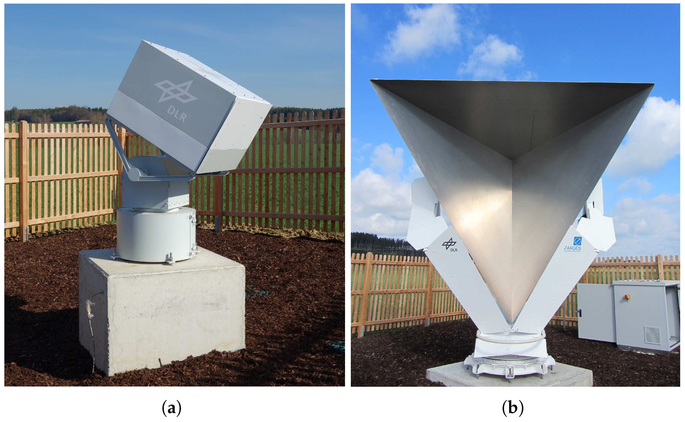
Figure 3.
DLR’s calibration site with three 2.8 m corner reflectors (D38, D42, D43) and three C-band transponders (D39, D40, D41) in South Germany with approximate center coordinate 48°0′N, 10°42′E. This calibration site is optimized for the Sentinel-1 mission, whereby the blue hatched areas indicate the Sentinel-1 coverage of all beams being selected for in-flight measurements (SM1, SM2, IW1, EW3, IW3, SM5, WV1).

Figure 4.
Sentinel-1 SAR image across the DLR calibration field in StripMap operation (SM5) for the co-polar channel VV. The regions around the deployed reference targets are zoomed out for the corresponding polarization channel (VV, VH).
Figure 4.
Sentinel-1 SAR image across the DLR calibration field in StripMap operation (SM5) for the co-polar channel VV. The regions around the deployed reference targets are zoomed out for the corresponding polarization channel (VV, VH).
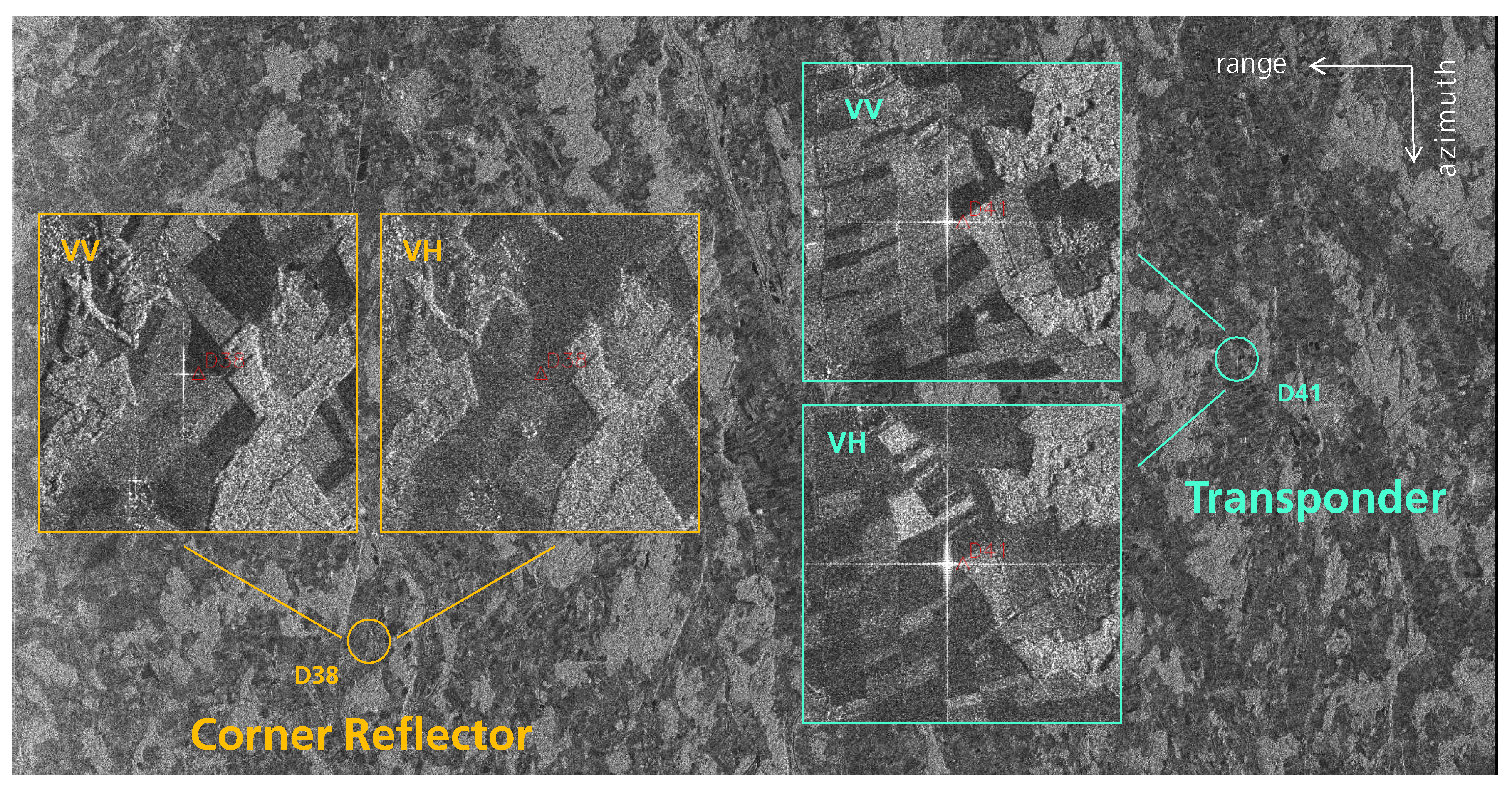
Figure 5.
Sentinel-1B front-end temperature drift (top plot); instrument drift in amplitude and in phase (middle and bottom plot) of the co-polar channel (VV) for a 25 min long IW data take acquired during the commissioning phase on 17 May 2016.
Figure 5.
Sentinel-1B front-end temperature drift (top plot); instrument drift in amplitude and in phase (middle and bottom plot) of the co-polar channel (VV) for a 25 min long IW data take acquired during the commissioning phase on 17 May 2016.

Figure 6.
Sentinel-1B instrument drift within a DT in amplitude (top plot) and phase (bottom plot) during the three months of CP from June to August 2016. Different colors indicate different acquisition modes.
Figure 6.
Sentinel-1B instrument drift within a DT in amplitude (top plot) and phase (bottom plot) during the three months of CP from June to August 2016. Different colors indicate different acquisition modes.
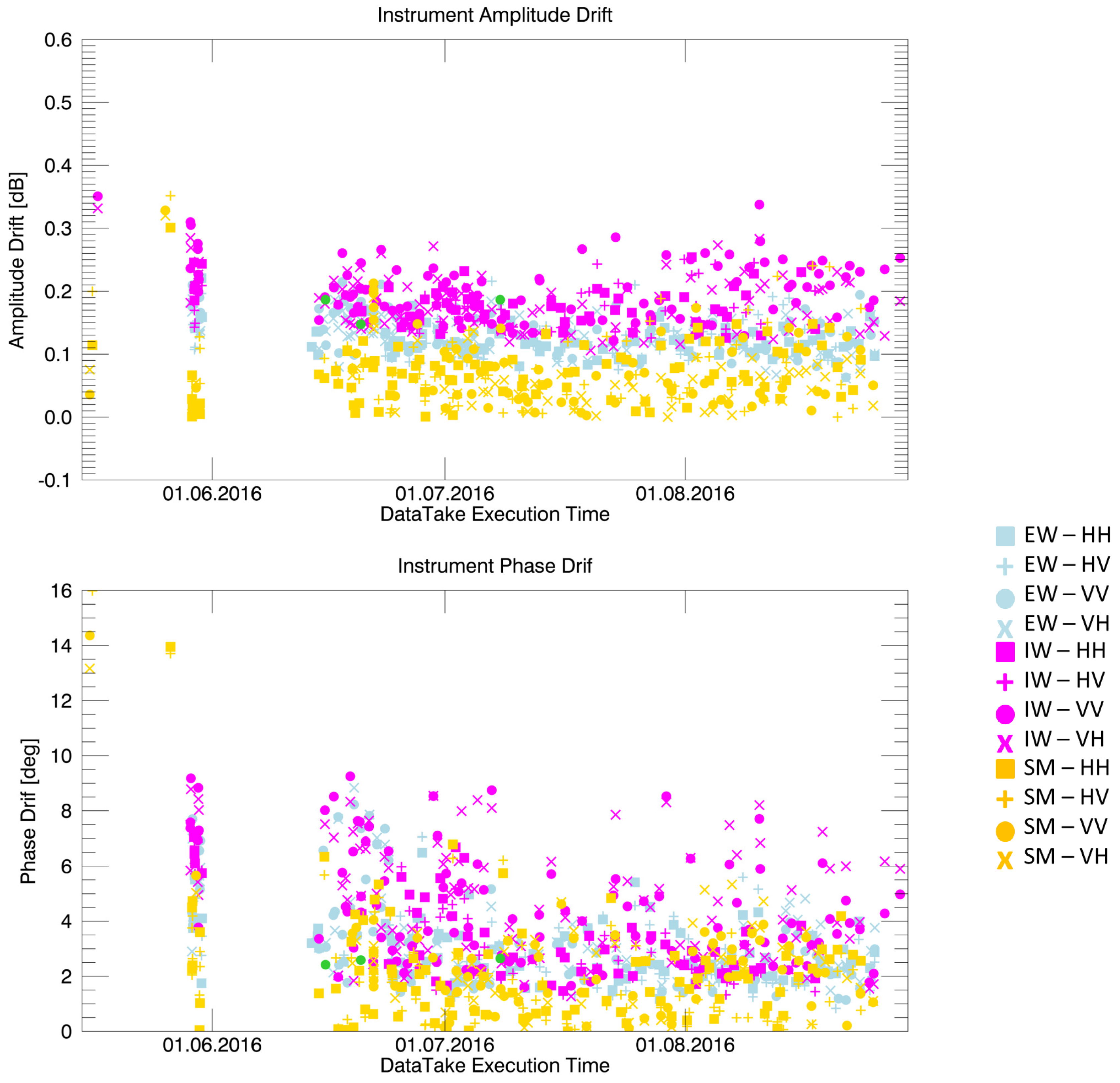
Figure 7.
Sentinel-1B instrument internal delay for the co- and cross-polar channels observed during the CP. Calibration pulses from the preamble (top plot) and postamble (bottom plot) have been evaluated on a daily basis during the CP.
Figure 7.
Sentinel-1B instrument internal delay for the co- and cross-polar channels observed during the CP. Calibration pulses from the preamble (top plot) and postamble (bottom plot) have been evaluated on a daily basis during the CP.

Figure 8.
Sentinel-1B PG Product amplitude and phase evaluation results during the Commissioning Phase.
Figure 8.
Sentinel-1B PG Product amplitude and phase evaluation results during the Commissioning Phase.
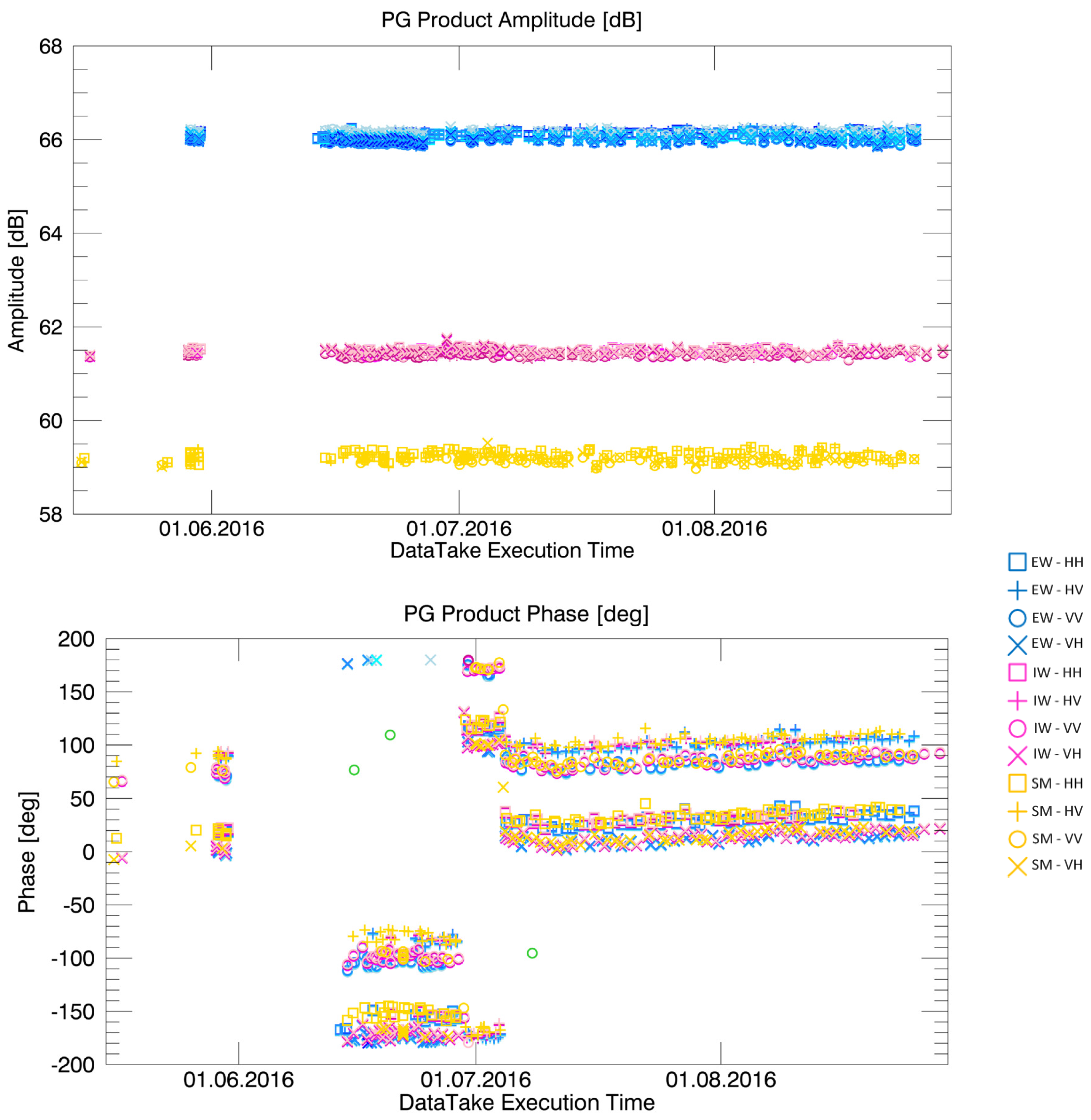
Figure 9.
Sentinel-1B Front-End mean temperature for the DTs analyzed during the CP.
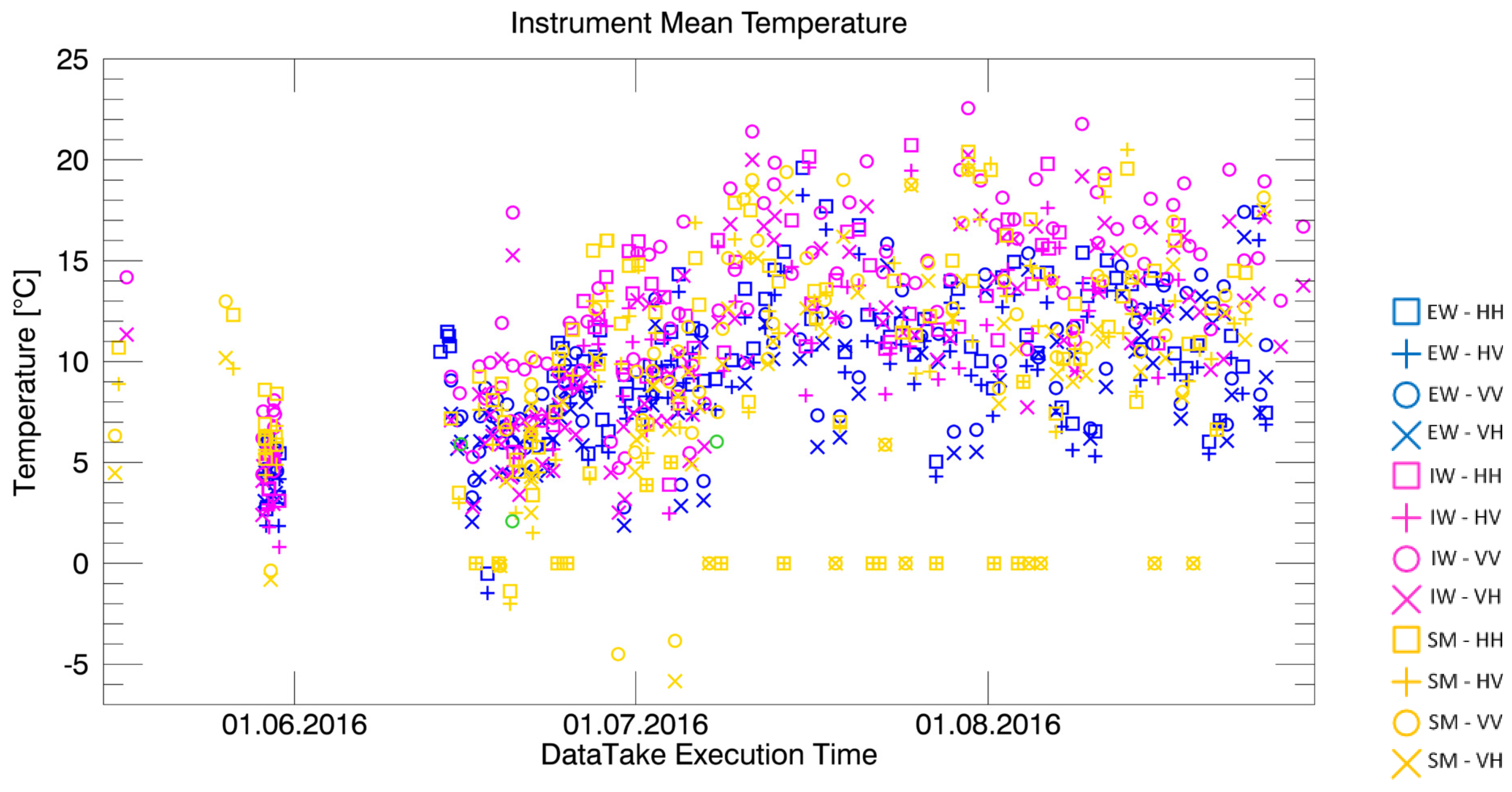
Figure 10.
Tx/Rx chain settings measured for individual Sentinel-1B front-end TRMs between June and August 2016. The blue curve represents the mean value of 76 RFC pairs per TRM for the V polarization.
Figure 10.
Tx/Rx chain settings measured for individual Sentinel-1B front-end TRMs between June and August 2016. The blue curve represents the mean value of 76 RFC pairs per TRM for the V polarization.

Figure 11.
Sentinel-1B front-end mean temperature during the 24 h of continuous RFC acquisitions, as part of the 24 h RFC campaign performed on 15 May 2016.
Figure 11.
Sentinel-1B front-end mean temperature during the 24 h of continuous RFC acquisitions, as part of the 24 h RFC campaign performed on 15 May 2016.
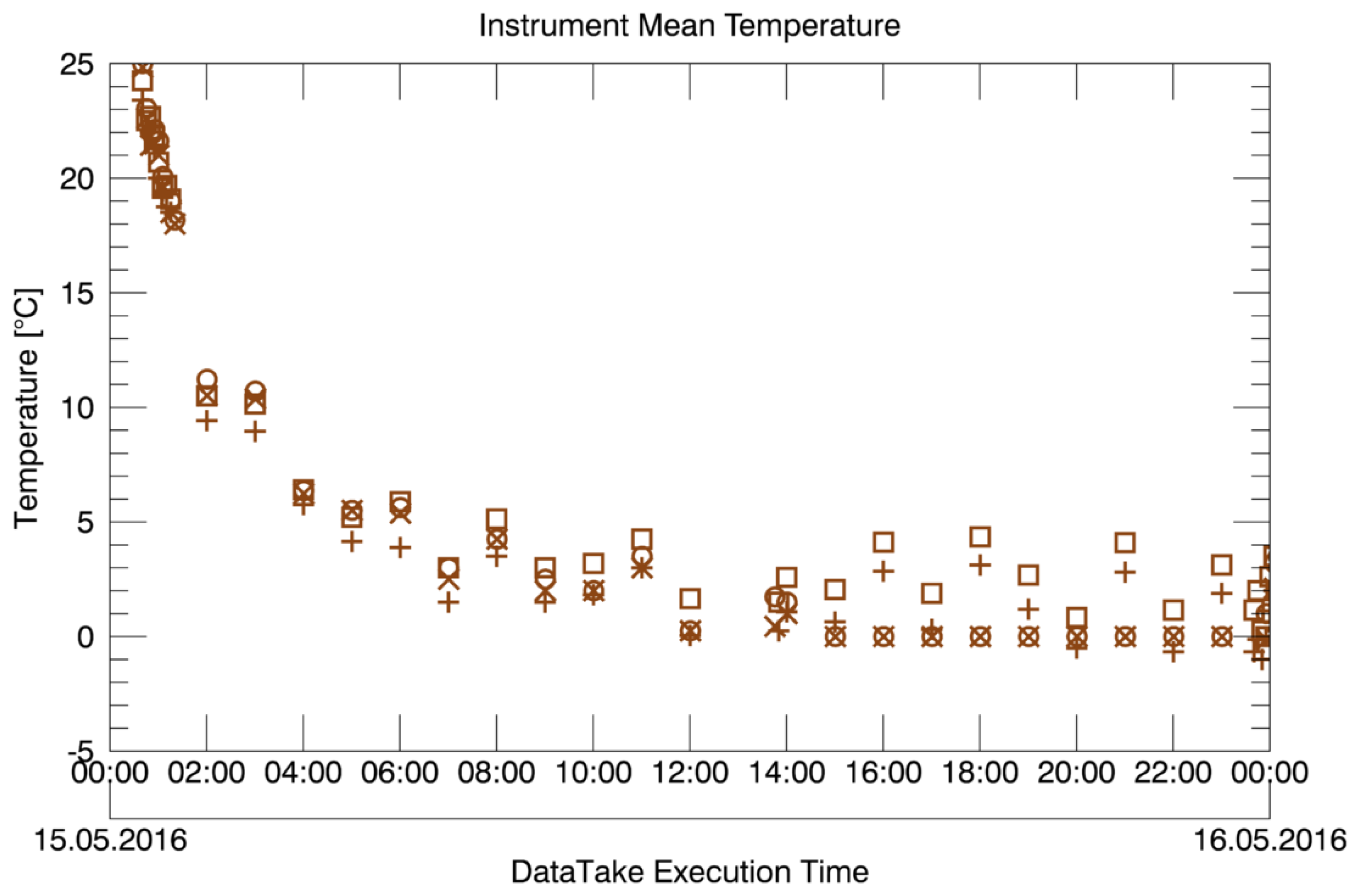
Figure 12.
Sentinel-1B amplitude and phase deviations for a total of 42 H-pol RFC measurements acquired during the 24 h RFC campaign in May 2016. The two top plots show the deviations for the Tx-chain (amplitude and phase); the two bottom plots show the deviations for the Rx chain.
Figure 12.
Sentinel-1B amplitude and phase deviations for a total of 42 H-pol RFC measurements acquired during the 24 h RFC campaign in May 2016. The two top plots show the deviations for the Tx-chain (amplitude and phase); the two bottom plots show the deviations for the Rx chain.
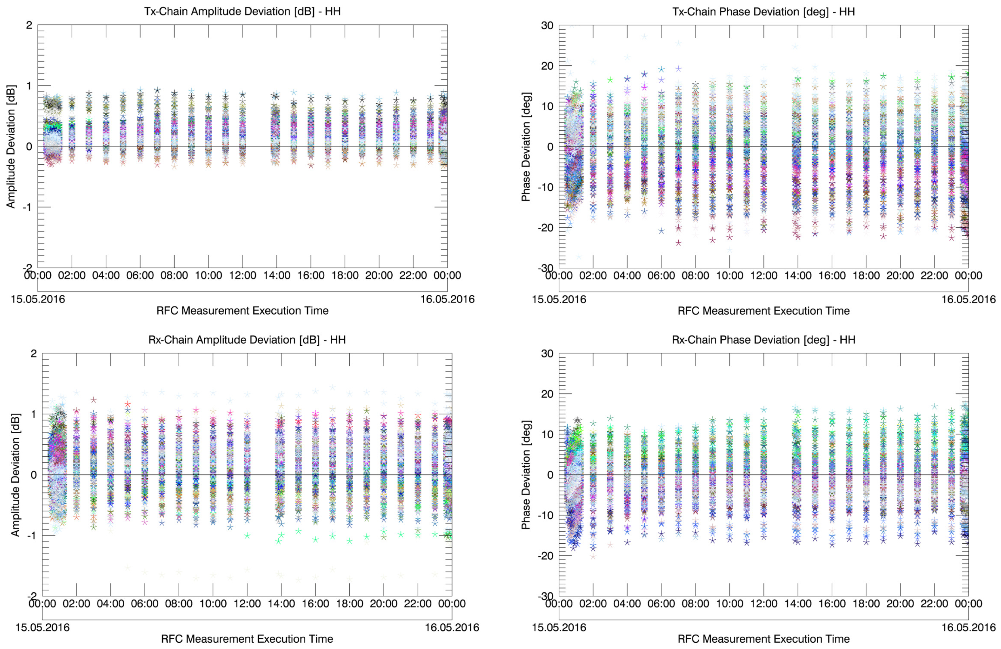
Figure 13.
Sentinel-1B amplitude and phase deviations w.r.t. the in-orbit reference for a total of 76 V-pol RFC measurements acquired between June and August 2016 during the CP. The two top plots show the deviations for the Tx-chain; the two bottom plots show the deviations for the Rx chain.
Figure 13.
Sentinel-1B amplitude and phase deviations w.r.t. the in-orbit reference for a total of 76 V-pol RFC measurements acquired between June and August 2016 during the CP. The two top plots show the deviations for the Tx-chain; the two bottom plots show the deviations for the Rx chain.
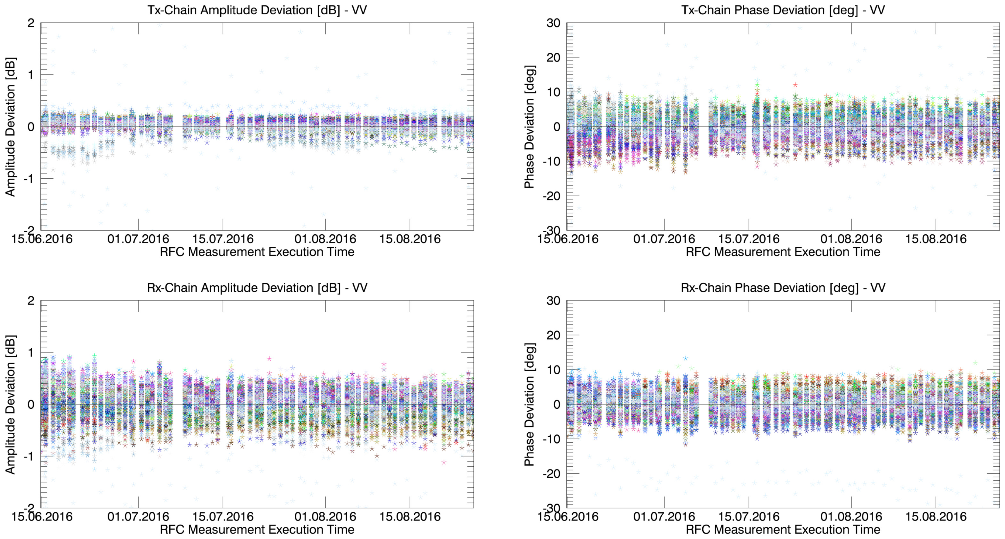
Figure 14.
Azimuth offset for all acquired overpasses derived from corner reflectors for SM (blue), IW (red) and EW mode (green).
Figure 14.
Azimuth offset for all acquired overpasses derived from corner reflectors for SM (blue), IW (red) and EW mode (green).
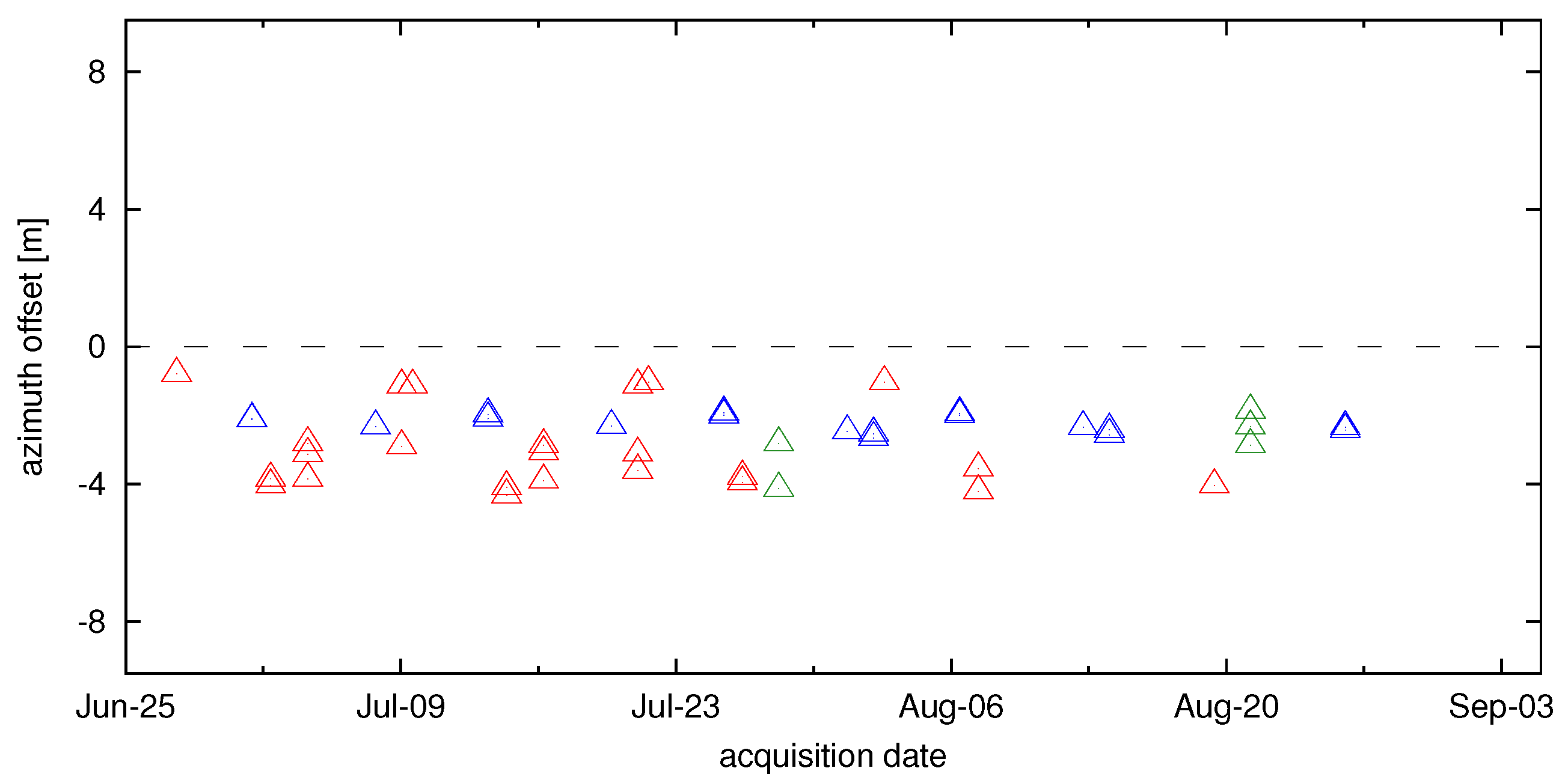
Figure 15.
Slant-range offset as a function of look angle derived from corner reflectors for the SM (blue), the IW (red) and the EW-mode (green); the instrument delay and propagation effects are already corrected.
Figure 15.
Slant-range offset as a function of look angle derived from corner reflectors for the SM (blue), the IW (red) and the EW-mode (green); the instrument delay and propagation effects are already corrected.

Figure 16.
Squint angle in azimuth as a function of the antenna look angle. The two dashed lines designate two separate fits to data which were acquired with two different star tracker configurations. Here, the change in configuration resulted in an offset in squint angle. N1–N6: azimuth notch acquisition with different look angles.
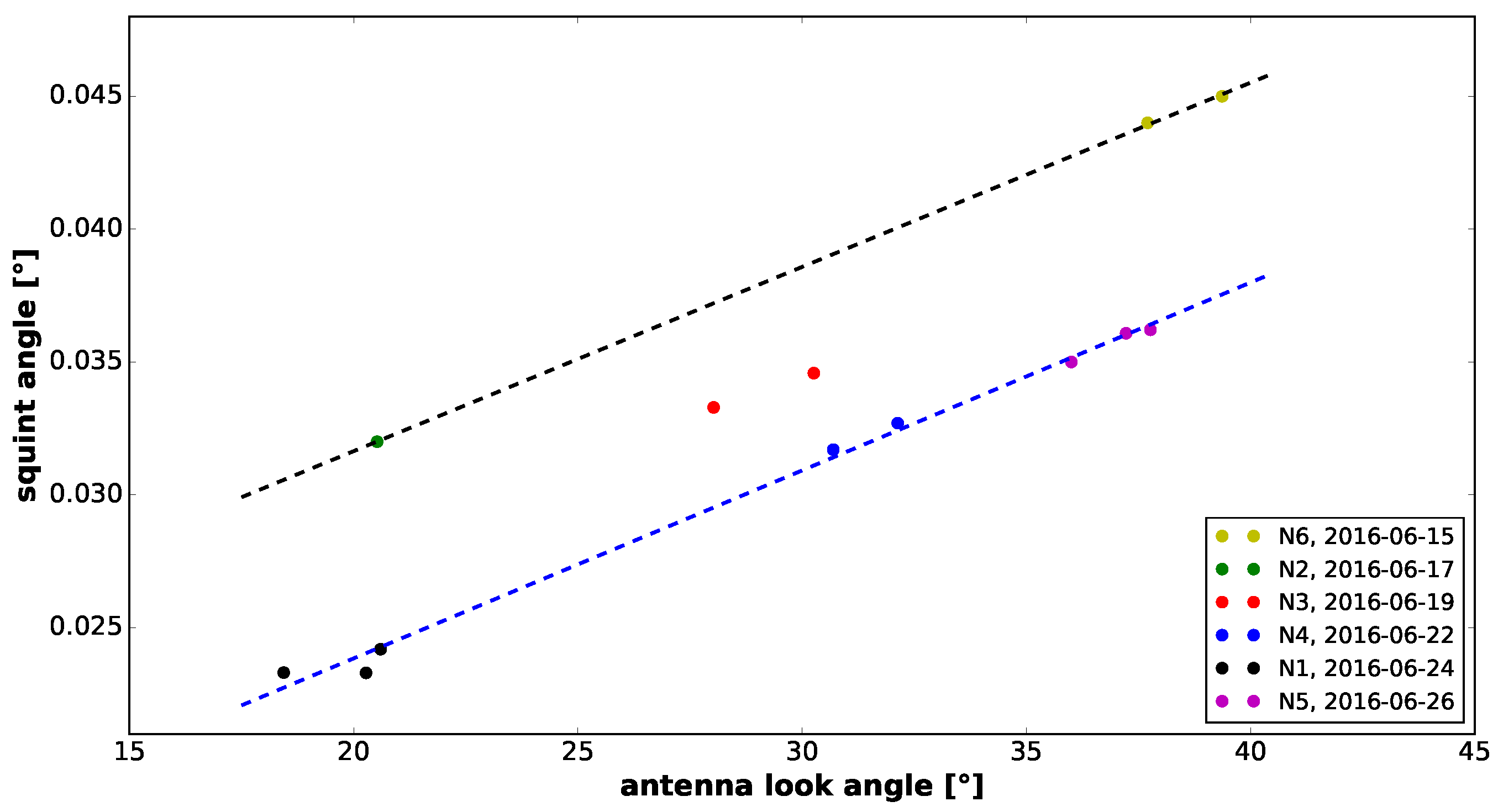
Figure 17.
Exemplary elevation notch beam evaluation for HH-Pol acquired on 19 June 2016. The blue curve in the plot on the left shows the full measured notch gamma profile. Marked in red is the central part of the notch which is used for minimum position determination. The plot on the right shows a detailed view of the central notch part (blue dots), a polynomial fit (polynomial of seventh order) based on this central part (red line) and the retrieved minimum position (red triangle) for HH-Pol.
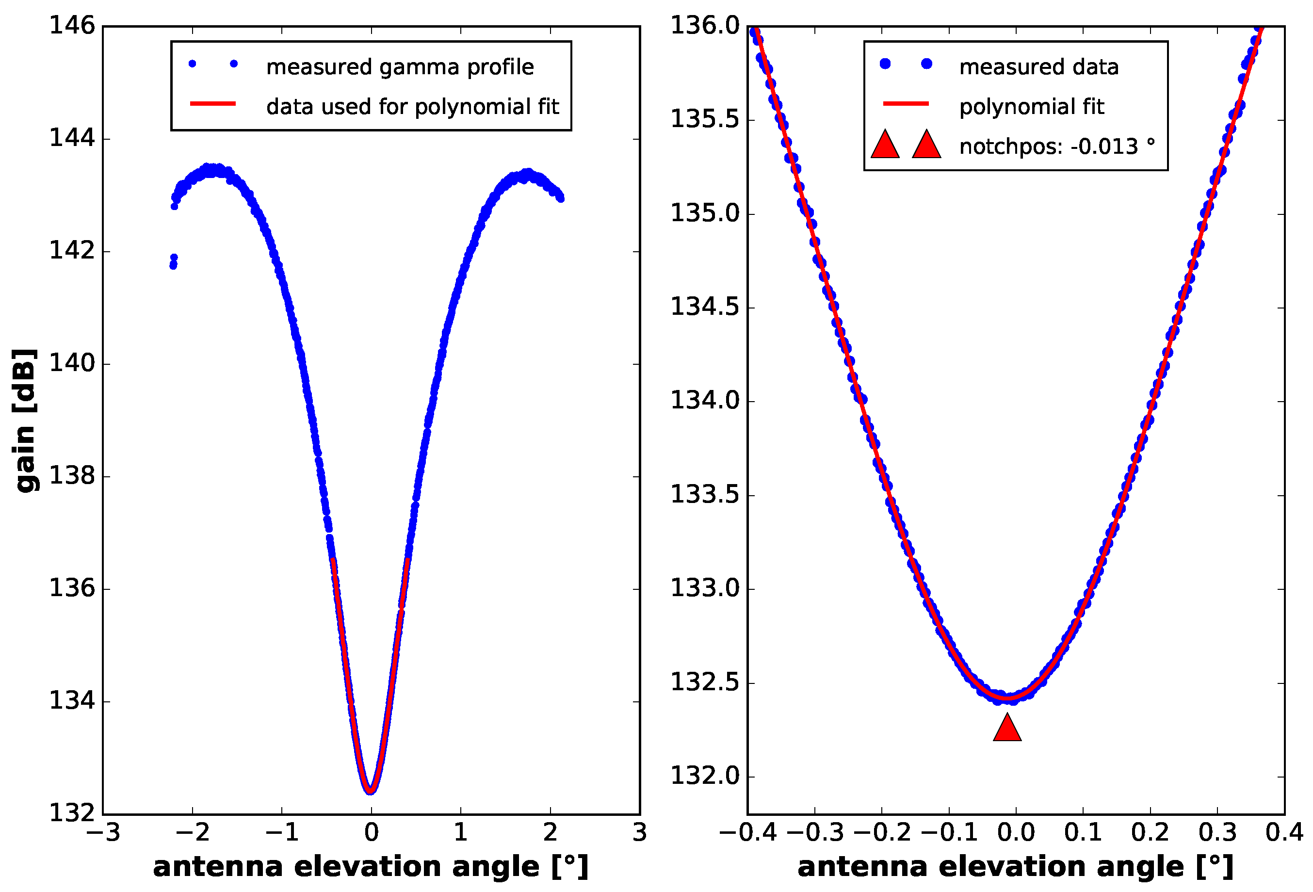
Figure 18.
Azimuth pattern measurement for SM2 on 29 June 2016, shifted to coincide at the maximum of the main beam. The top plot shows the sidelobes as a function of azimuth angles. The bottom plot shows a zoom of the measurement/model difference over the main lobe area and the deviation between the averaged measured patterns; the calculated reference is shown in black.

Figure 19.
Averaged IW gamma profiles measured after star tracker realignment shown without antenna pattern compensation (solid lines) for co-pol (top plot) and cross-pol (bottom plot) and the corresponding antenna model predictions (dashed lines). The antenna model prediction has been adjusted using an offset defined by the difference between the mean modeled and mean measured IW3 gain. Hence, the beam-to-beam differences can be compared with respect to IW3 for both model and measurement.
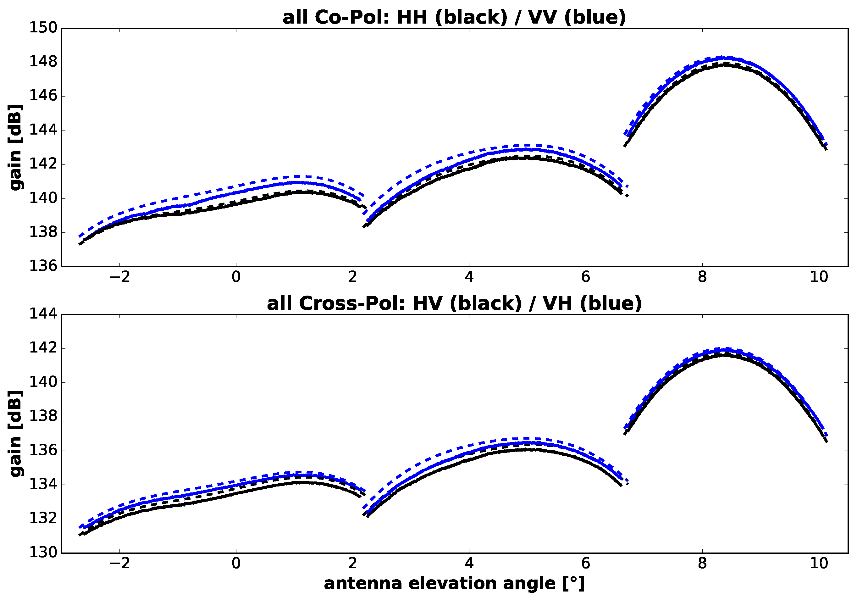
Figure 20.
IW3-mean-removed difference between averaged measured IW data and the corresponding antenna model prediction after star tracker realignment.
Figure 20.
IW3-mean-removed difference between averaged measured IW data and the corresponding antenna model prediction after star tracker realignment.

Figure 21.
Plot analogue to Figure 19 for averaged EW measurements. Here, the antenna model prediction has been adjusted using the offset defined by the difference between the mean modeled and mean measured EW3 gain. Hence, the beam-to-beam differences can be compared with respect to EW3 for both model and measurement.

Figure 22.
EW3-mean-removed difference between averaged measured EW data and the corresponding antenna model prediction. The distinct monotonous variation over elevation for each sub-swath signifies a potential influence of antenna mispointing.
Figure 22.
EW3-mean-removed difference between averaged measured EW data and the corresponding antenna model prediction. The distinct monotonous variation over elevation for each sub-swath signifies a potential influence of antenna mispointing.

Figure 23.
Timeline of the standard deviation of the absolute calibration factor for each overpass for all acquired products (blue: SM, red: IW, green: EW) for co-polarization channels. The number of covered targets within the scene is denoted in the circle center.
Figure 23.
Timeline of the standard deviation of the absolute calibration factor for each overpass for all acquired products (blue: SM, red: IW, green: EW) for co-polarization channels. The number of covered targets within the scene is denoted in the circle center.

Figure 24.
Absolute calibration factor for co-polarized channels using different targets (triangle: corner reflectors, square: transponders) acquired for different modes (blue: SM, red: IW, green: EW).
Figure 24.
Absolute calibration factor for co-polarized channels using different targets (triangle: corner reflectors, square: transponders) acquired for different modes (blue: SM, red: IW, green: EW).

Figure 25.
Channel imbalance between the cross- and co-polar channel derived from the transponder IRF for H- (filled diamonds HV-HH in dB) and V-polarization (open diamonds VH-VV in dB) on transmit for different modes (blue: SM, red: IW, green: EW).
Figure 25.
Channel imbalance between the cross- and co-polar channel derived from the transponder IRF for H- (filled diamonds HV-HH in dB) and V-polarization (open diamonds VH-VV in dB) on transmit for different modes (blue: SM, red: IW, green: EW).

Figure 26.
Channel imbalance between the cross- and co-polar channel derived from rainforest EW mode acquisitions for H on transmit (black) and V on transmit (blue). The channel imbalance is plotted for two cases: using the standard SLC products including the antenna pattern correction (blue and black lines) and without antenna pattern correction (green and purple lines).

Figure 27.
Cross-talk derived from DLR corner reflectors for different modes (blue: SM, red: IW, green: EW).
Figure 27.
Cross-talk derived from DLR corner reflectors for different modes (blue: SM, red: IW, green: EW).

Figure 28.
Mean Doppler centroid frequencies of Sentinel-1A and 1B units during the Sentinel-1B commissioning phase.
Figure 28.
Mean Doppler centroid frequencies of Sentinel-1A and 1B units during the Sentinel-1B commissioning phase.
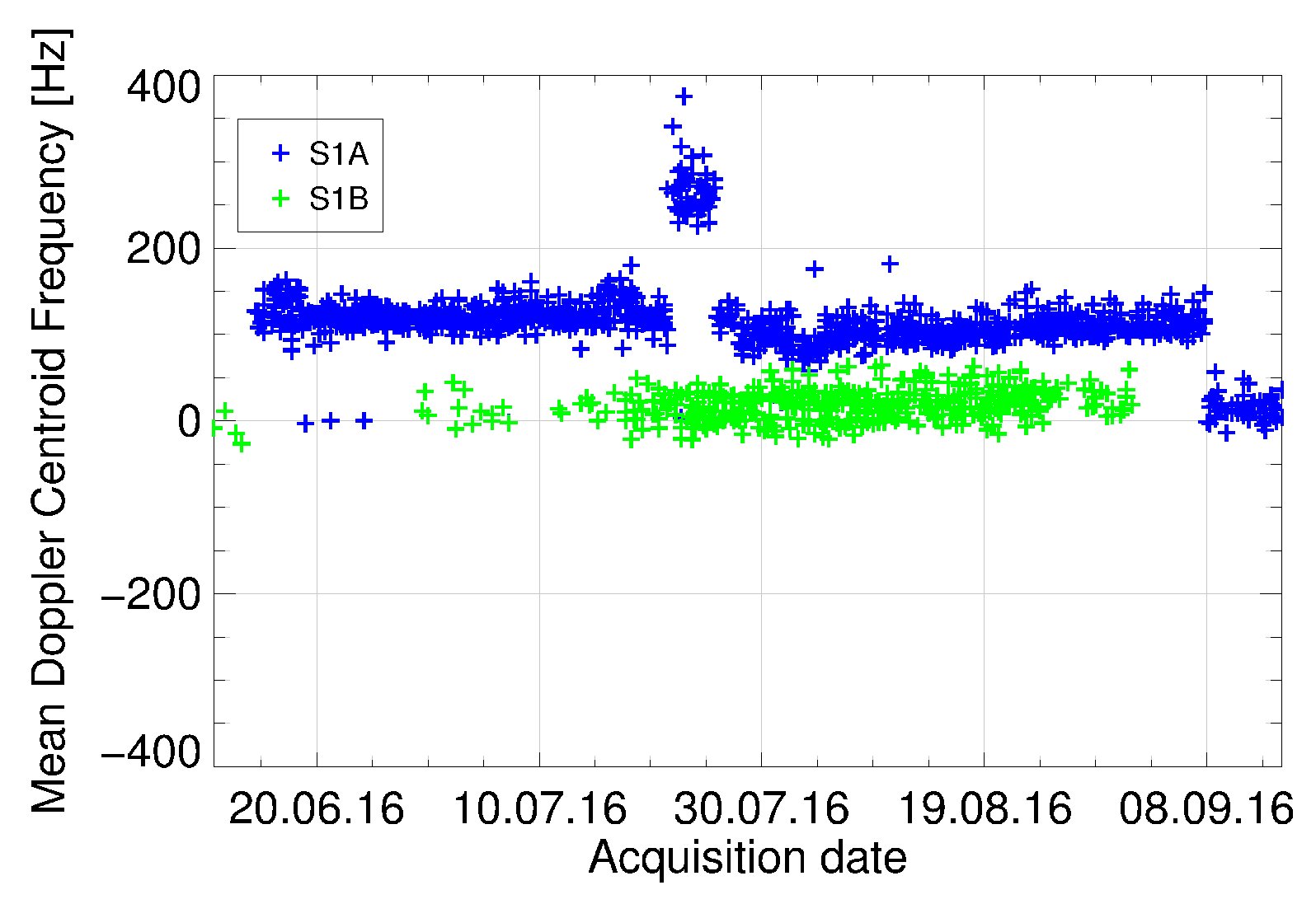
Figure 29.
InSAR baselines, burst mis-synchronization and final common Doppler bandwidth for the combination of S1B–S1B (first column) and S1B–S1A (second column) InSAR data pairs. The first row shows the physical baseline (B), perpendicular baseline (), and parallel baseline () for all analyzed pairs, as a function of the geographic latitude. The second row shows the burst mis-synchronization values of the analyzed pairs. The third row shows the percentage of the final common Doppler bandwidth with the master acquisition date.
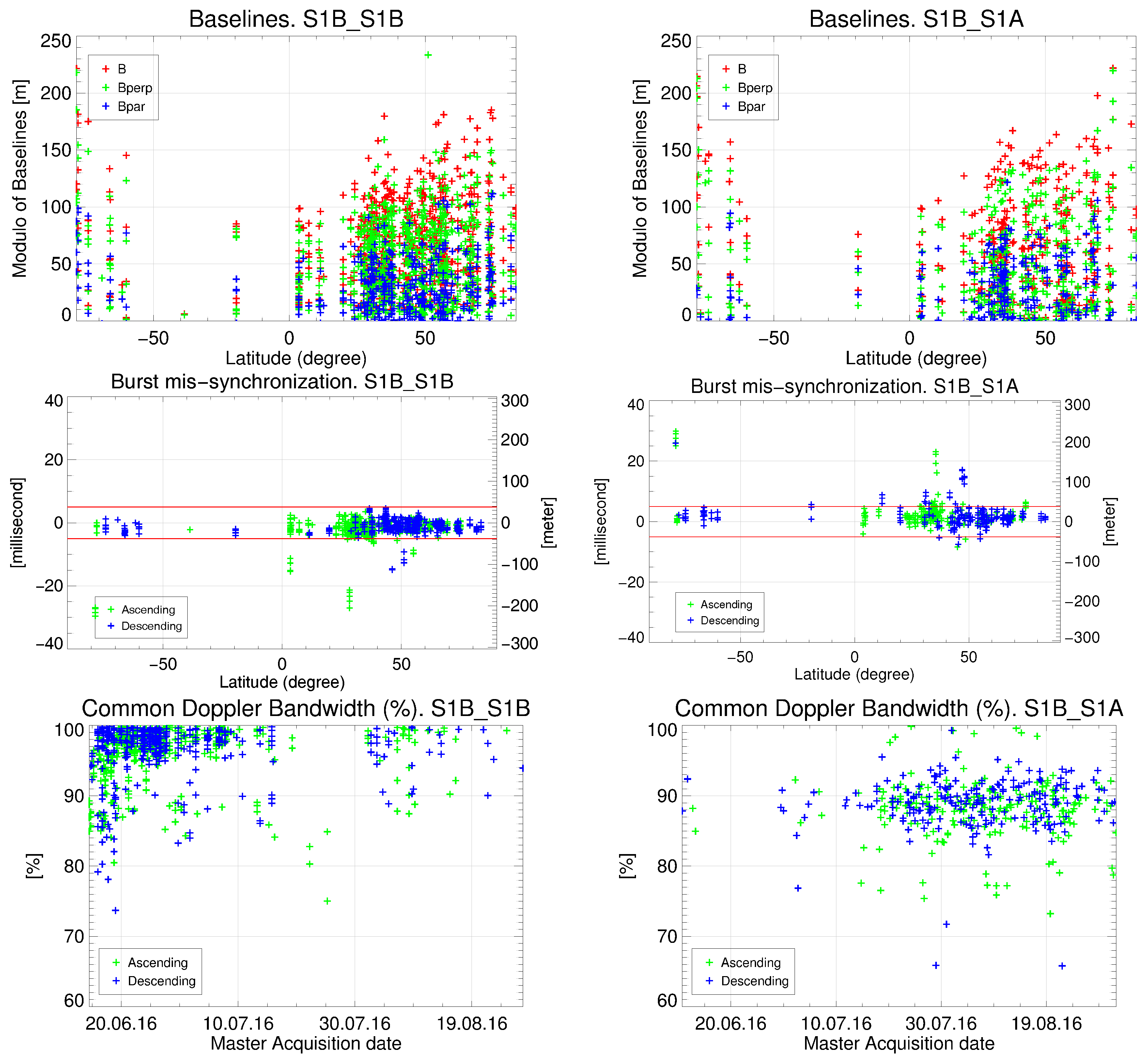
Figure 30.
Sentinel-1A/B cross-interferogram acquired over east Europe for a long data take (range is vertical, azimuth is horizontal): (top) Reflectivity image; (middle) coherence and (bottom) DEM-flattened interferometric phase. The Sentinel-1A/B images were acquired on 13 June (S1A) and 19 June 2016 (S1B). The data take consists of eight slices with a total of 72 bursts and is about 1400 km long. The data take duration was 3 min and 20 s. The residual fringes observed in the interferogram are mainly related to atmospheric artifacts.
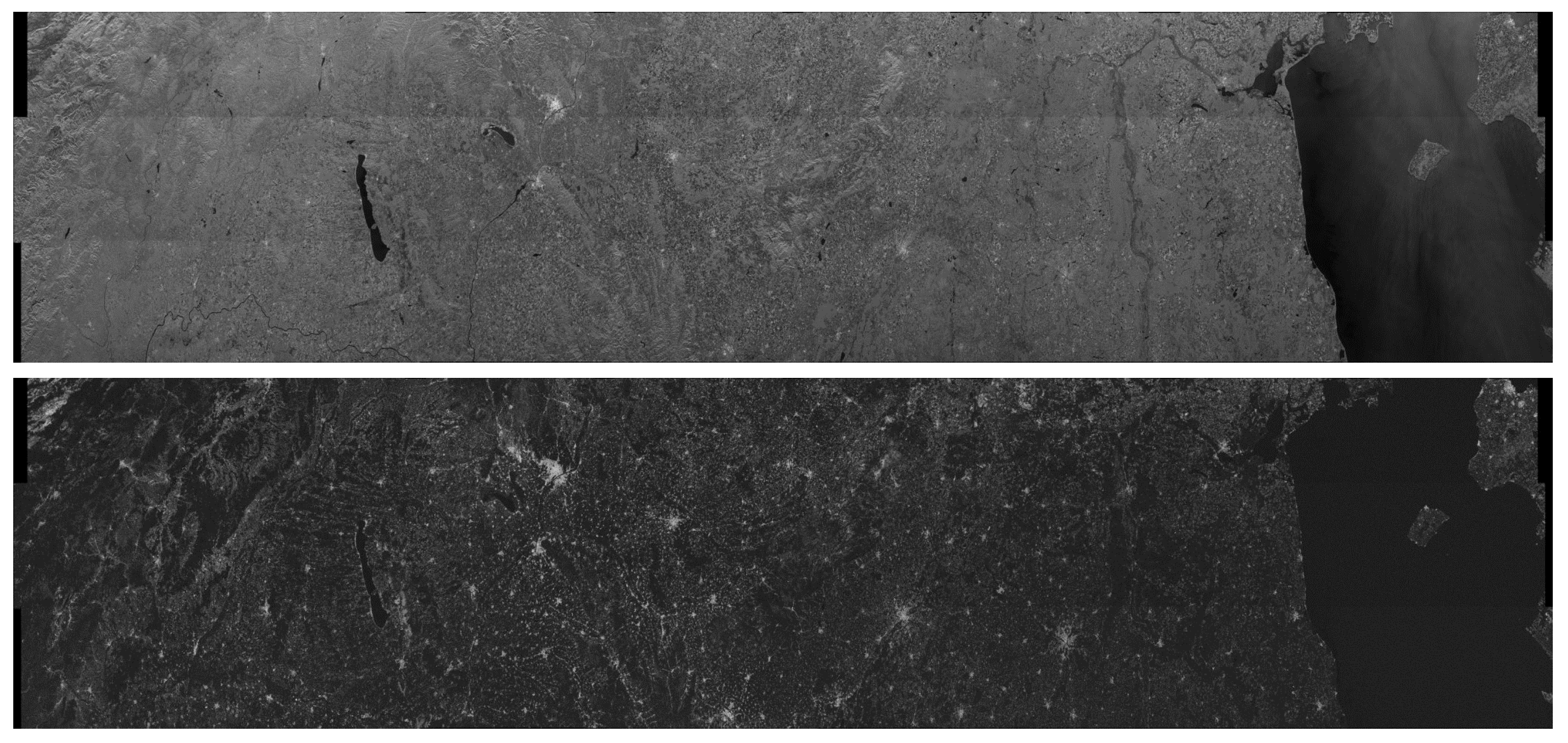

Figure 31.
Measured azimuth mis-registration between master and slave images by using the enhanced spectral diversity (ESD) approach [22] for every overlap area of the data take.
Figure 31.
Measured azimuth mis-registration between master and slave images by using the enhanced spectral diversity (ESD) approach [22] for every overlap area of the data take.
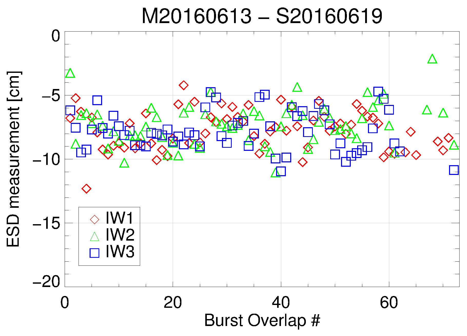
Figure 32.
Absolute calibration factor derived from point targets for the IW mode (triangle: corner reflectors, square: co- transponders, crosses: cross- transponder) and distinguished between transmit polarization (blue: H on transmit, red: V on transmit). (a) for Sentinel-1B of the IW mode; (b) for Sentinel-1A of the IW mode.
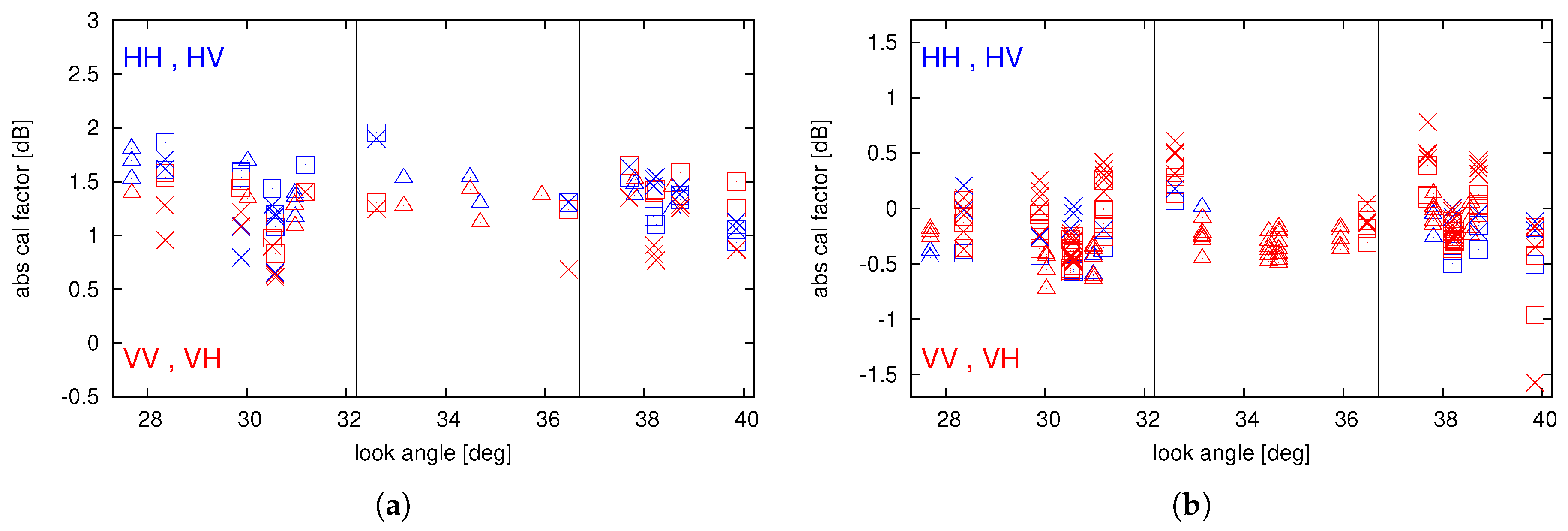

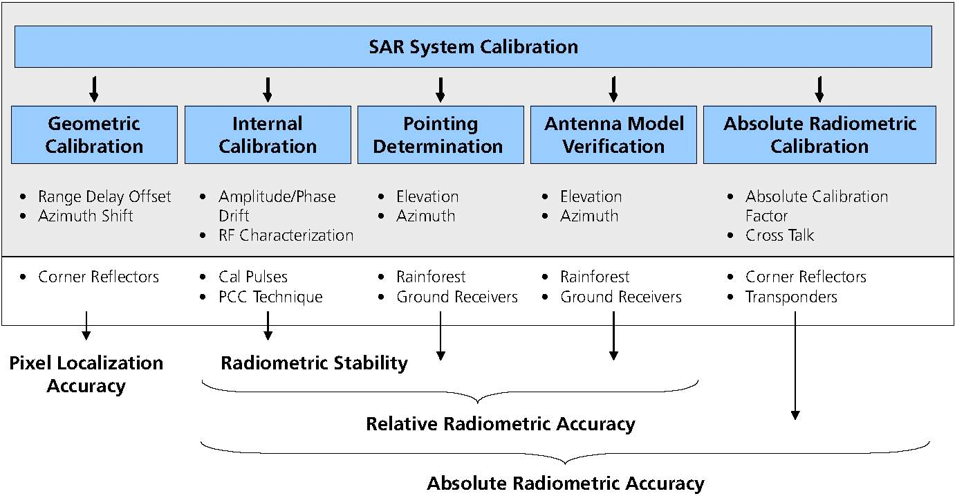
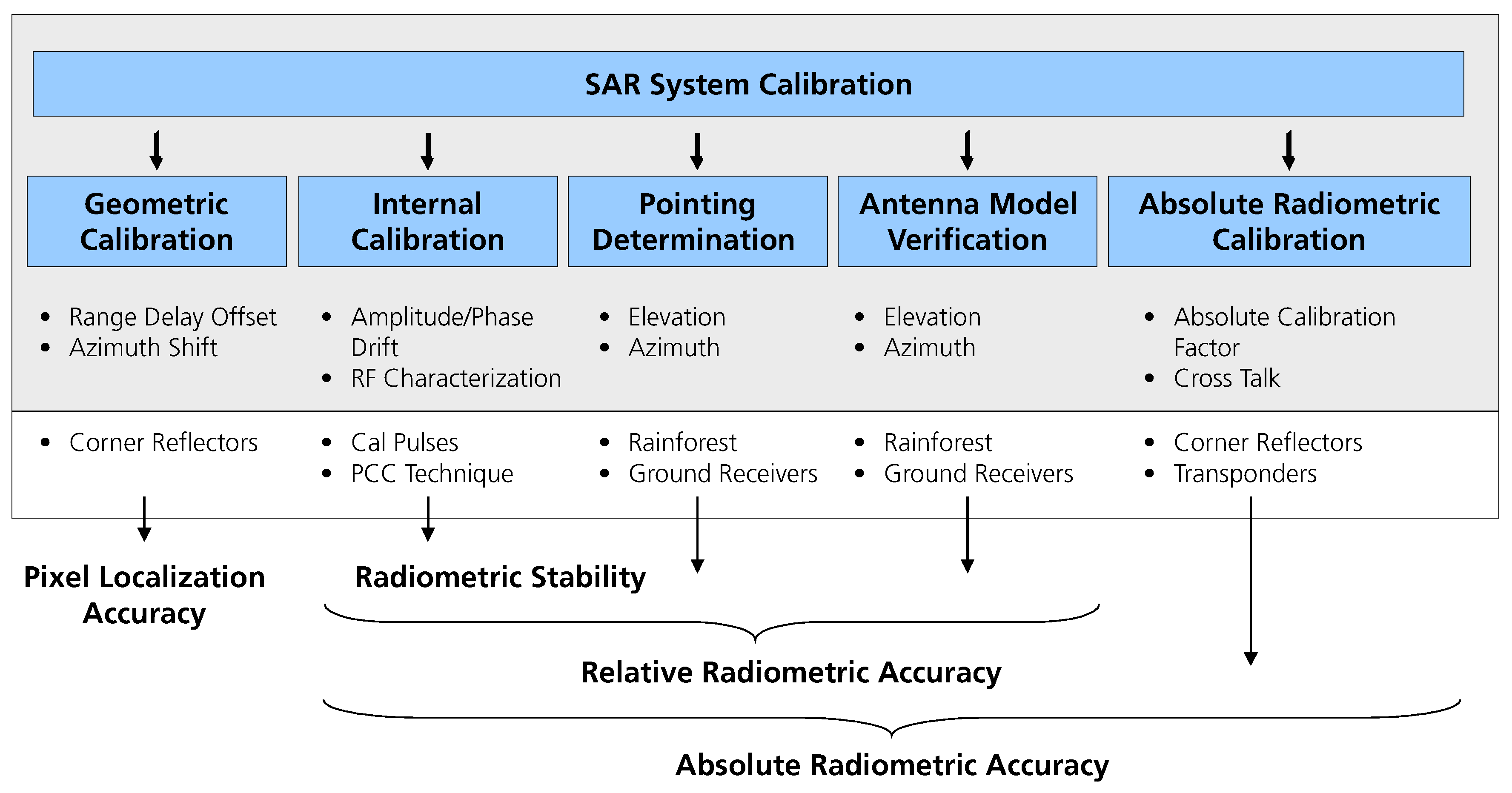
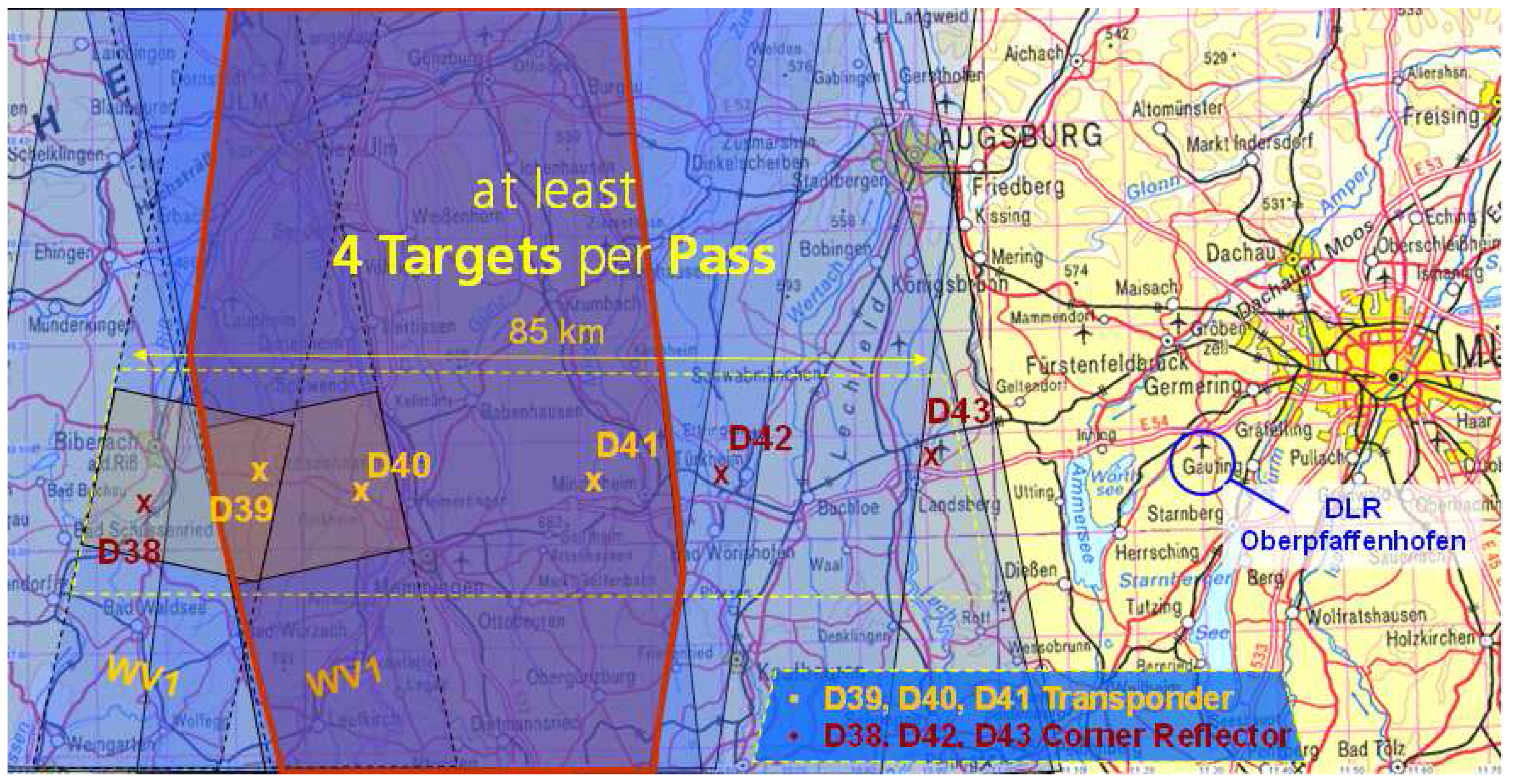
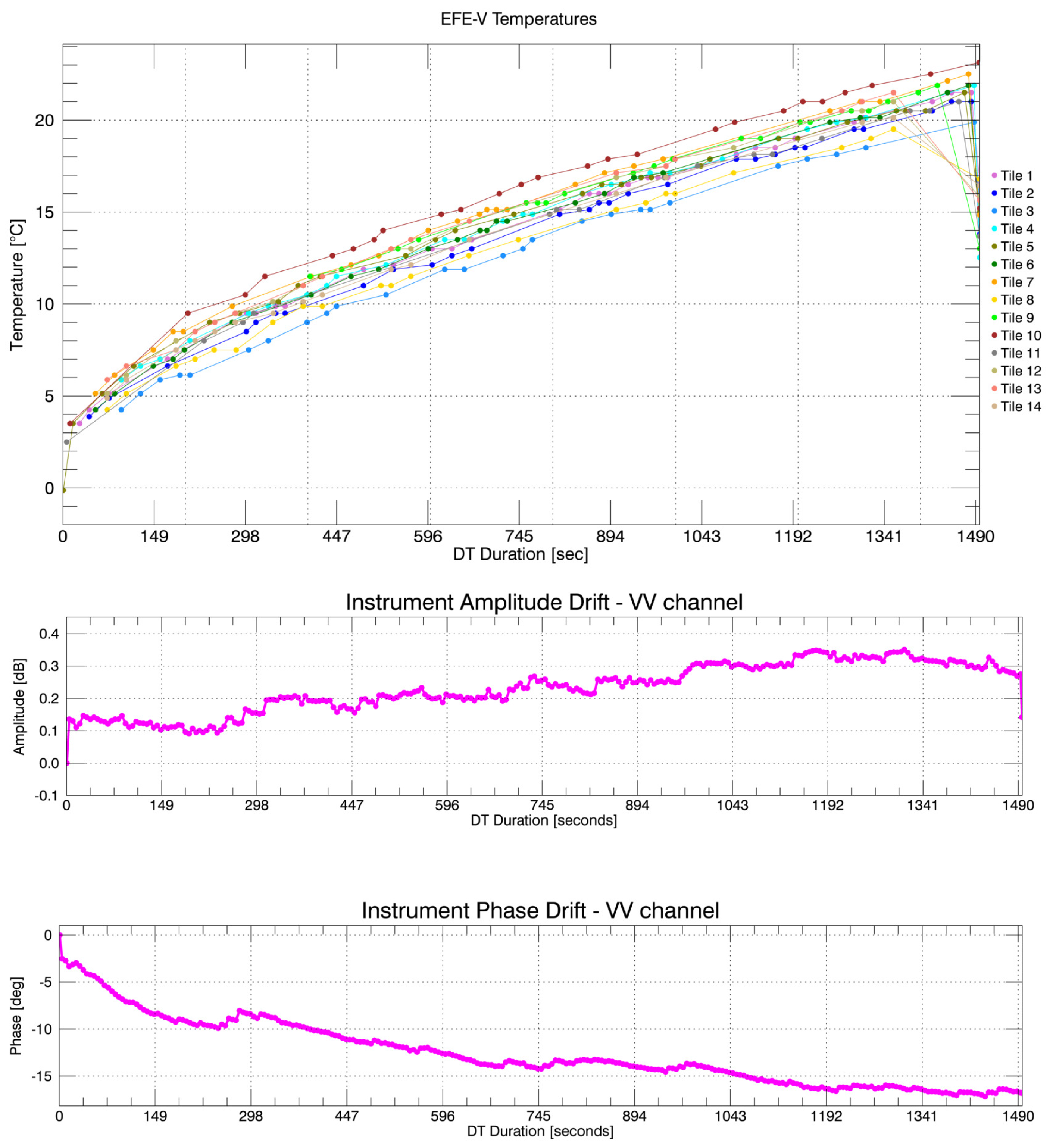
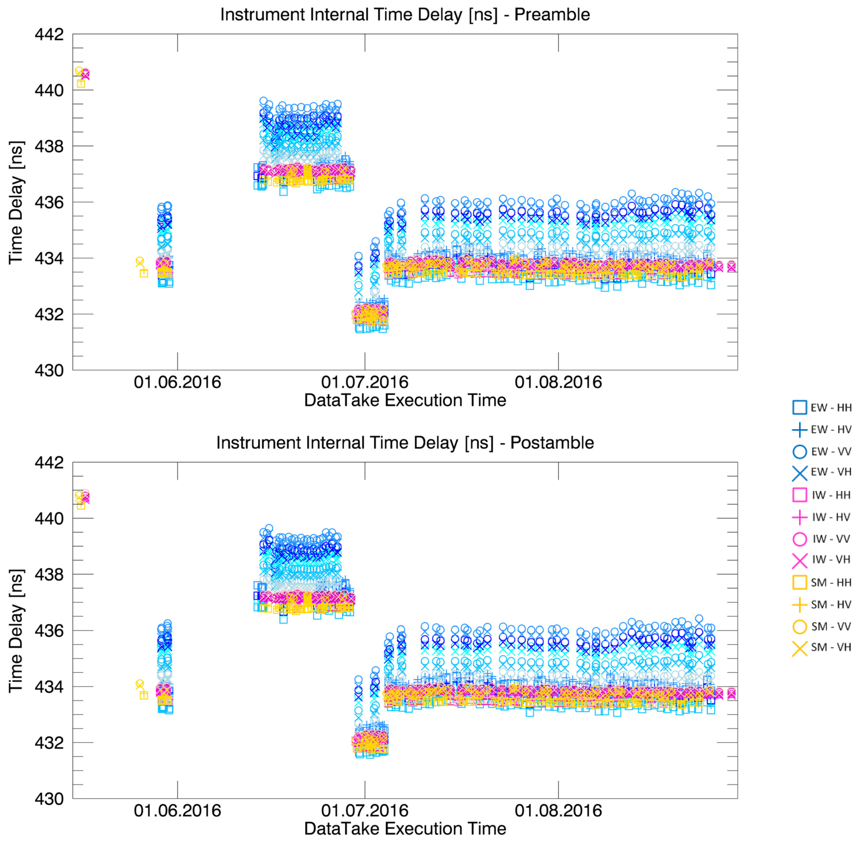
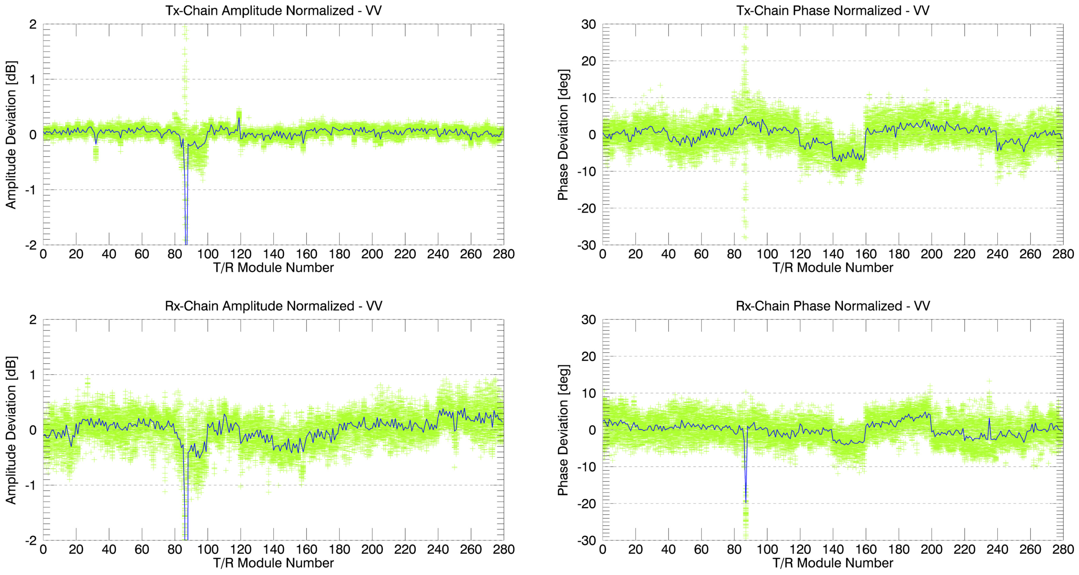
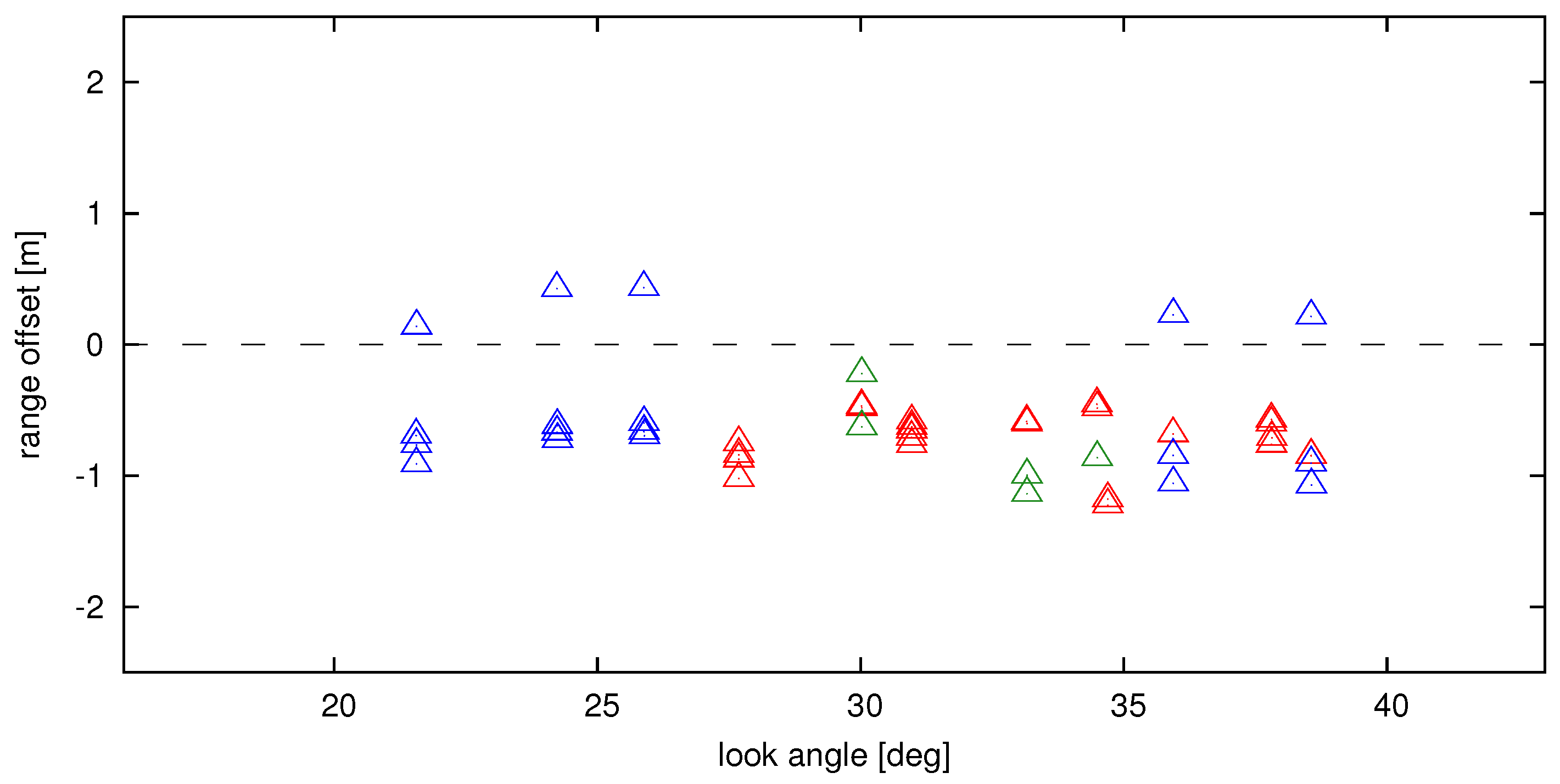
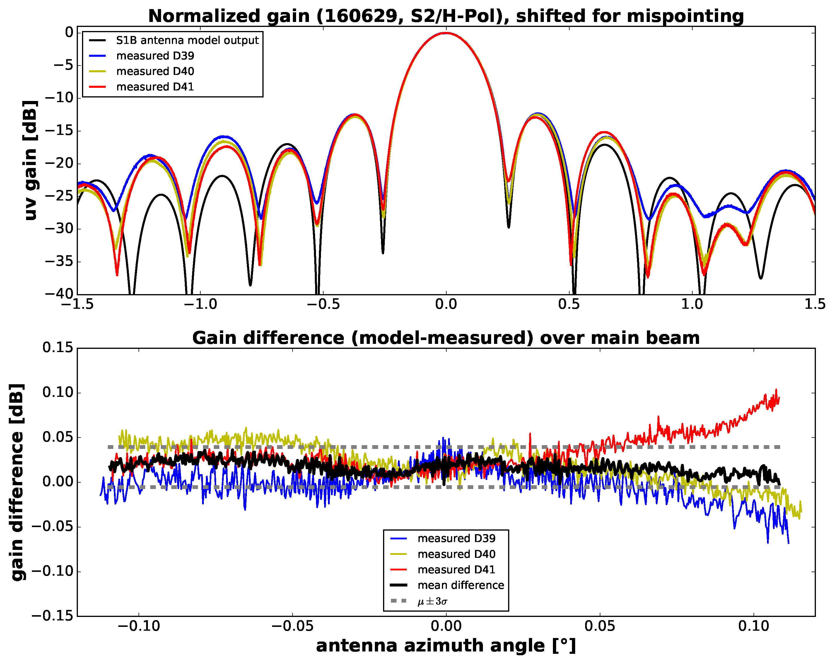
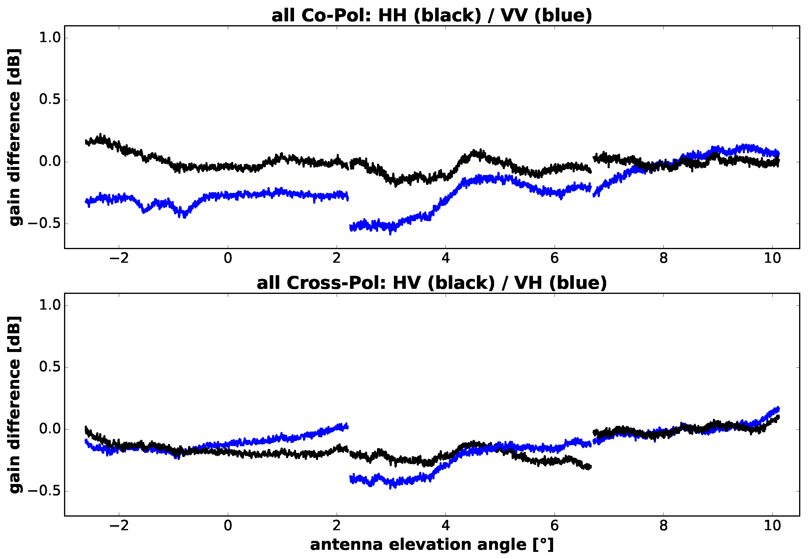
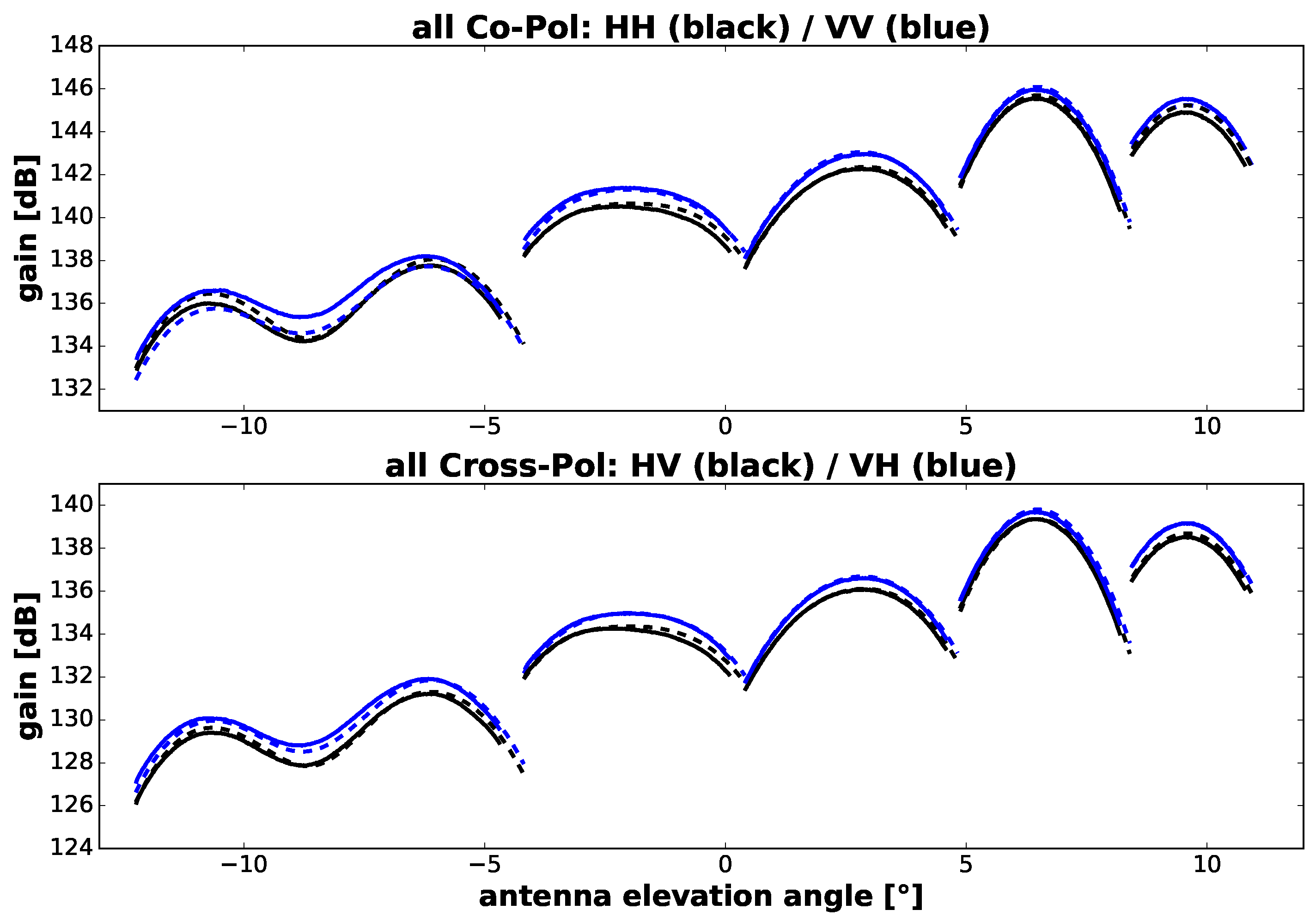
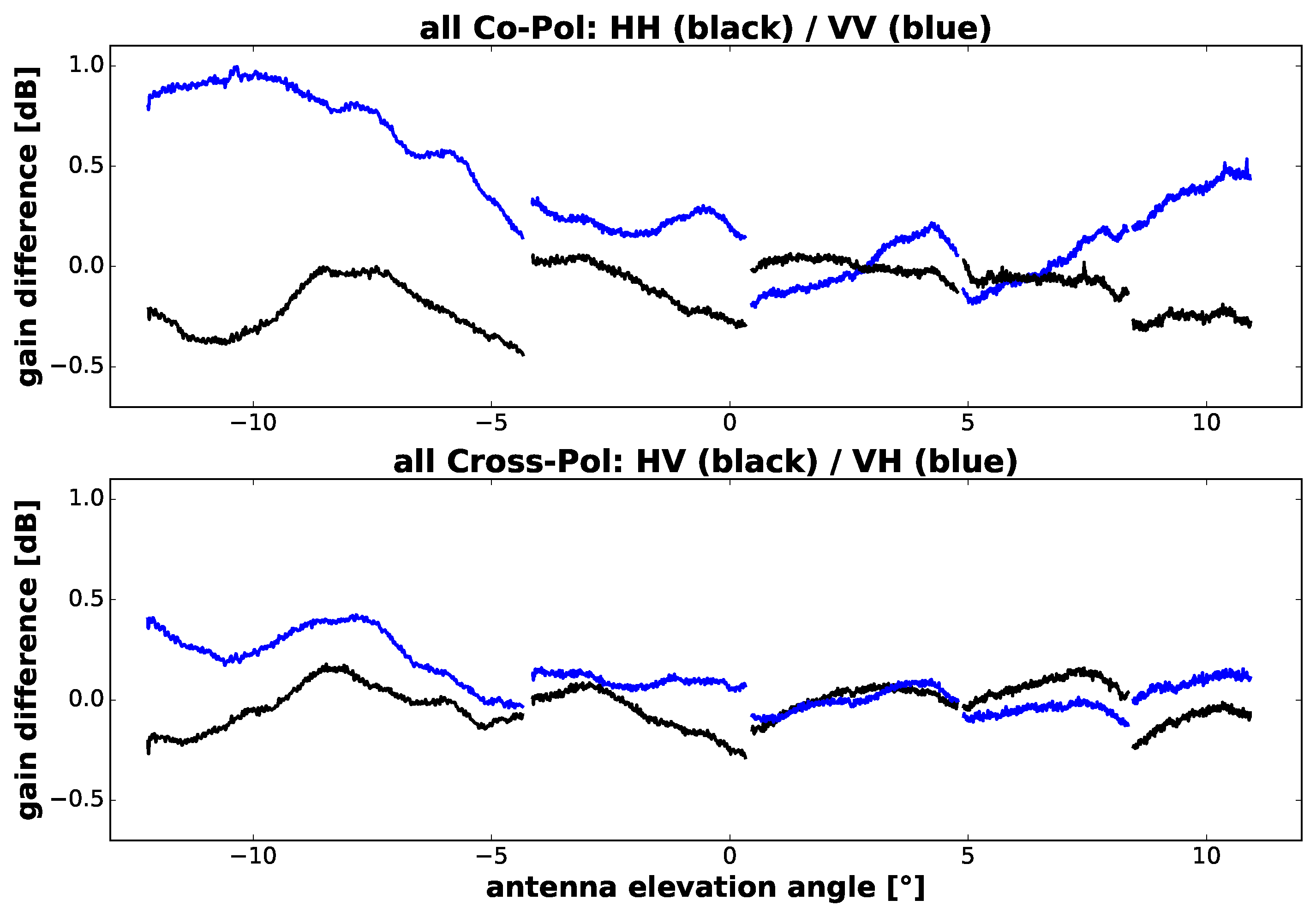
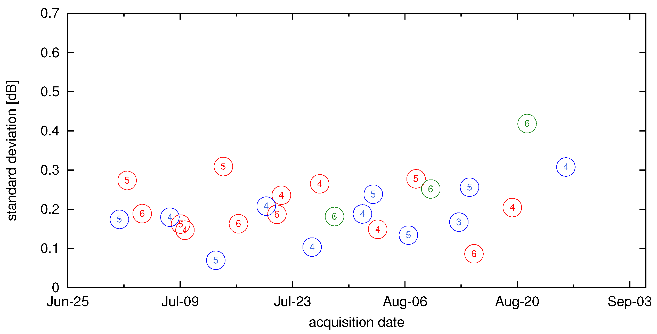
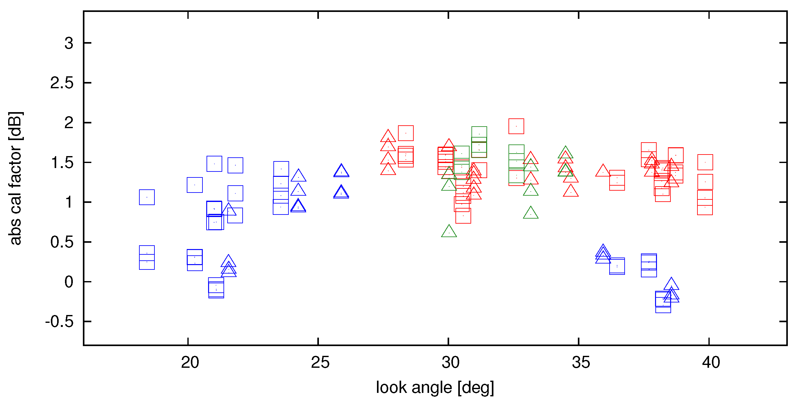
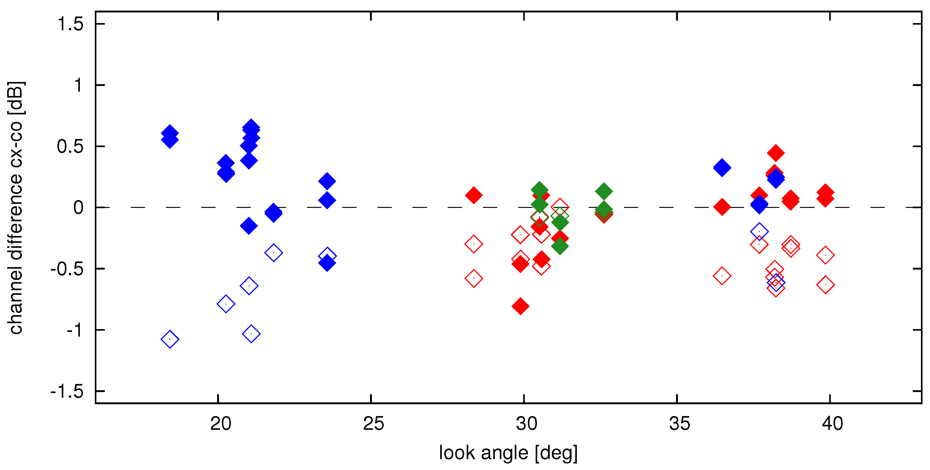
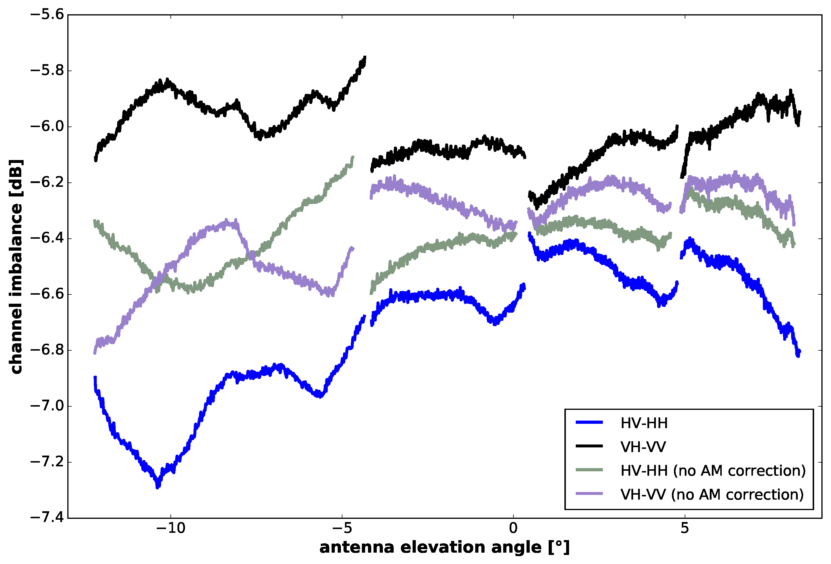
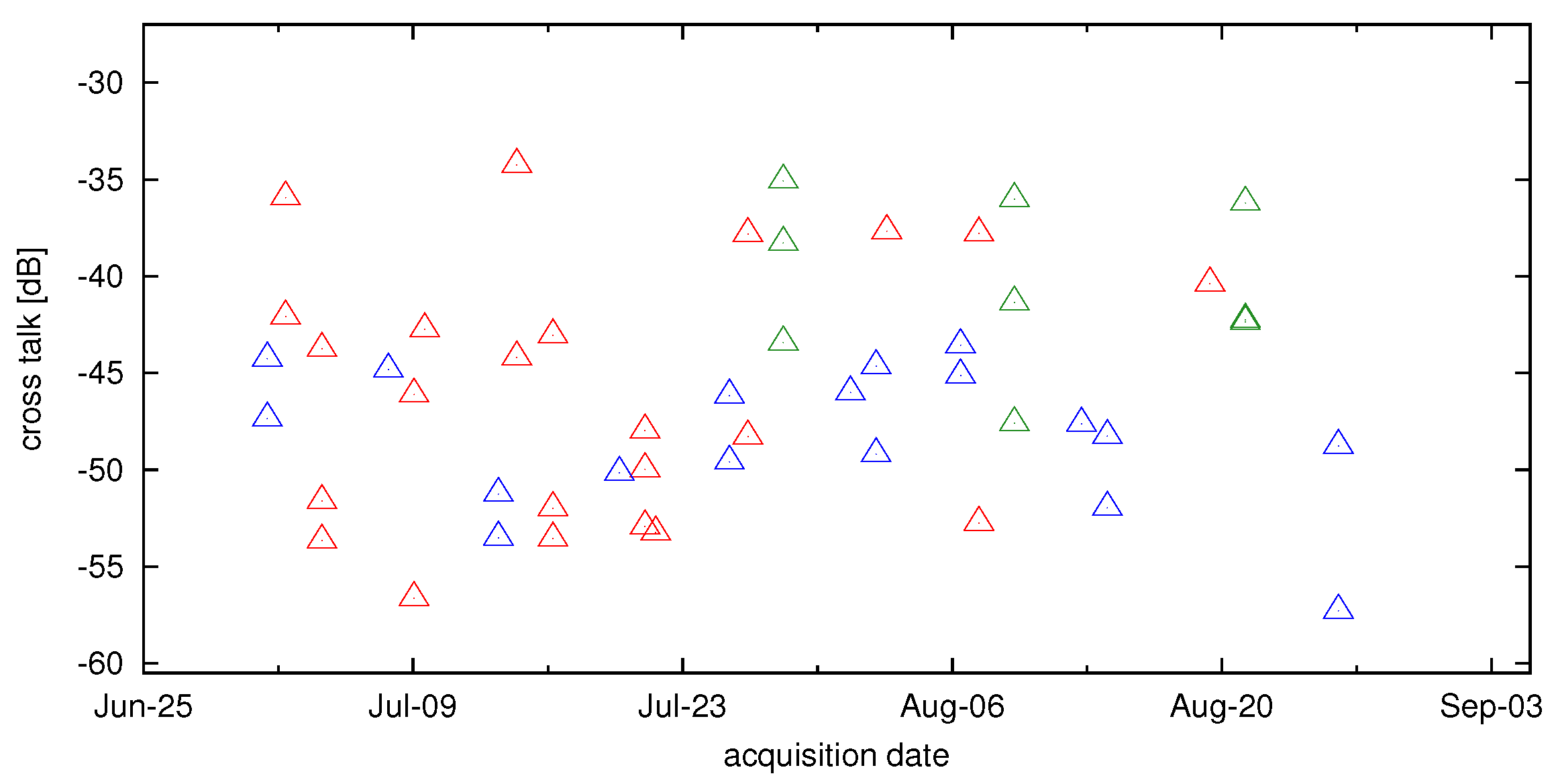
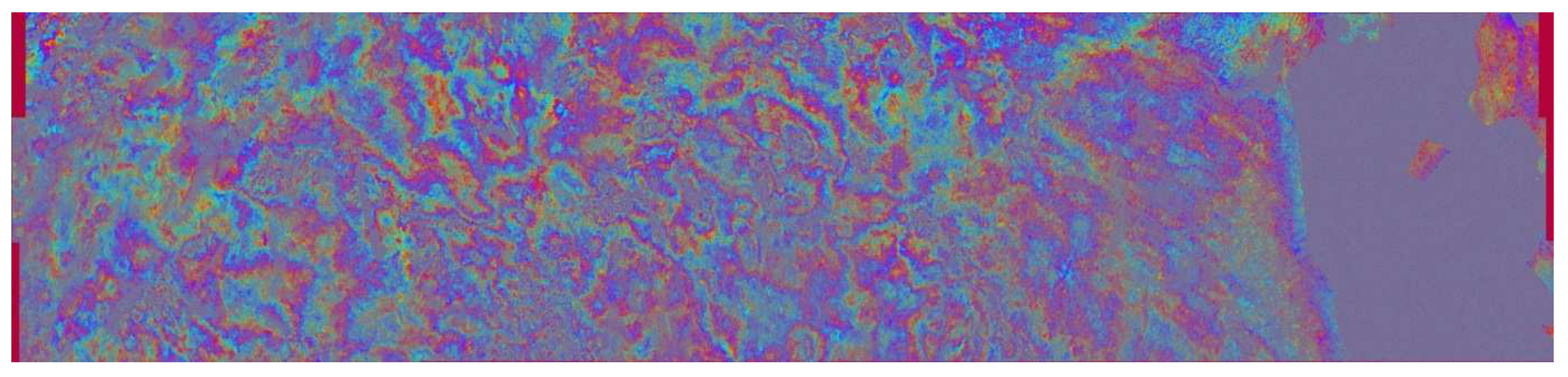
Table 1.
Sentinel-1B instrument amplitude and phase drift for long DTs acquired with different polarizations and acquisition modes.
Table 1.
Sentinel-1B instrument amplitude and phase drift for long DTs acquired with different polarizations and acquisition modes.
| IW | SM6 | SM6 | |
|---|---|---|---|
| Polarization | DV | DH | DV |
| Date | 17 May 2016 | 26 May 2016 | 25 May 2016 |
| Duration | 25 min | 25 min | 25 min |
| Mean Temp. | 14 C | 12 C | 13 C |
| Temp. Drift | 23 C | 20 C | 23 C |
| Amp. Drift | 0.25 dB | 0.2 dB | 0.23 dB |
| Phase Drift | 17.2 | 13.9 | 19.6 |
Table 2.
Sentinel-1B instrument internal delay for long DTs acquired with different polarizations and acquisition modes.
Table 2.
Sentinel-1B instrument internal delay for long DTs acquired with different polarizations and acquisition modes.
| Data Take | Swath | PREAMBLE | POSTAMBLE | Time Delay |
|---|---|---|---|---|
| SM DH | SM6 | 433.91 ns | 434.11 ns | 0.2 ns |
| 100 MHz | 433.70 ns | 433.81 ns | 0.11 ns | |
| SM DV | SM6 | 433.46 ns | 433.68 ns | 0.22 ns |
| 100 MHz | 433.51 ns | 433.65 ns | 0.14 ns | |
| Mean Value | 433.64 ns | 433.81 ns | 0.17 ns | |
| Standard Deviation | 0.18 ns | 0.18 ns | 0.04 ns | |
Table 3.
Geometric offsets and pixel localization accuracy in azimuth and in range for different SAR modes derived from DLR corner reflectors.
Table 3.
Geometric offsets and pixel localization accuracy in azimuth and in range for different SAR modes derived from DLR corner reflectors.
| Mode | Azimuth Offset | Range Offset | ||
|---|---|---|---|---|
| [m] | [m] | [m] | [m] | |
| SM | −2.2 | 0.2 | −0.5 | 0.5 |
| IW | −3.0 | 1.2 | −0.7 | 0.2 |
| EM | −2.8 | 0.8 | −0.7 | 0.3 |
| all | −2.7 | 1.0 | −0.6 | 0.4 |
Table 4.
Antenna elevation mispointing values, i.e., differences between measured notch positions and antenna model prediction, derived from all elevation notch measurements acquired after the star tracker realignment.
Table 4.
Antenna elevation mispointing values, i.e., differences between measured notch positions and antenna model prediction, derived from all elevation notch measurements acquired after the star tracker realignment.
| Datatake ID | Measurement Date | Pass | Polarization | Mispointing [mdeg] |
|---|---|---|---|---|
| 2283/1 (A495) | 13 August 2016 | asc. | HH | −11 |
| 2283/2 (3D2F) | 13 August 2016 | asc. | HH | −11 |
| 2283/3 (F631) | 13 August 2016 | asc. | HH | −13 |
| 2283/4 (4932) | 13 August 2016 | asc. | HH | −21 |
| 2380/1 (5279) | 15 August 2016 | desc. | VV | −16 |
| 2380/2 (9CBA) | 15 August 2016 | desc. | VV | −17 |
| 25D2/1 (A9C4) | 18 August 2016 | asc. | HH | −13 |
| 25D2/2 (ED0E) | 18 August 2016 | asc. | HH | −13 |
| 25D2/3 (05D5) | 18 August 2016 | asc. | HH | −13 |
| 25D2/4 (B0C9) | 18 August 2016 | asc. | HH | −19 |
| 26F5/2 (3311) | 20 August 2016 | asc. | VV | −18 |
| 26F5/3 (52FF) | 20 August 2016 | asc. | VV | −18 |
| 26F5/4 (DF60) | 20 August 2016 | asc. | VV | −16 |
| −15 ± 3 |
Table 5.
Overview of all results achieved for StripMap azimuth pattern verification.
| Measurement Date | Swath Type | Transmit Polarization | Model-Measured over Main Beam/ [dB] |
|---|---|---|---|
| 29 June 2016 | SM2 | H | 0.035 (3 transponder average) |
| 6 July 2016 | SM1 | H | 0.031 (1 transponder) |
| 11 July 2016 | SM2 | V | 0.023 (3 transponder average) |
| 18 July 2016 | SM1 | V | 0.032 (3 transponder average) |
| 30 July 2016 | SM1 | H | 0.019 (3 transponder average) |
| 1 August 2016 | SM5 | H | 0.026 (3 transponder average) |
| 4 August 2016 | SM2 | H | 0.015 (1 transponder) |
| 11 August 2016 | SM1 | H | 0.042 (1 transponder) |
| 13 August 2016 | SM5 | H | 0.008 (3 transponder average) |
Table 6.
Mean value and standard deviation of the absolute calibration factor for the beams measured in-flight by separating co- and cross-channel results and summarizing all polarization channels.
Table 6.
Mean value and standard deviation of the absolute calibration factor for the beams measured in-flight by separating co- and cross-channel results and summarizing all polarization channels.
| Mode | Co-Channels (HH, VV) | Cross-Channels (HV, VH) | All Channels (HH, HV, VV, VH) | |||
|---|---|---|---|---|---|---|
| [dB] | [dB] | [dB] | [dB] | [dB] | [dB] | |
| S1 | 0.39 | 0.45 | 0.49 | 0.35 | 0.44 | 0.41 |
| S2 | 1.13 | 0.23 | 1.12 | 0.18 | 1.13 | 0.21 |
| S5 | 0.07 | 0.25 | 0.10 | 0.43 | 0.08 | 0.31 |
| IW (1,2,3) | 1.40 | 0.23 | 1.17 | 0.33 | 1.31 | 0.29 |
| EM (2,3) | 1.40 | 0.30 | 1.54 | 0.14 | 1.45 | 0.26 |
Table 7.
Standard deviation of the geometrical baselines for the S1B–S1B and S1B–S1A pairs.
| Physical Baseline (B) | Perp. Baseline () | Parallel Baseline () | |
|---|---|---|---|
| S1B–S1B. Standard deviation | 94.4 m | 81.22 m | 63.67 m |
| S1B–S1A. Standard deviation | 105.82 m | 89.43 m | 73.35 m |
Table 8.
Standard deviation of the radial and cross-track orbit components for S1B pairs and S1B–S1A combination.
Table 8.
Standard deviation of the radial and cross-track orbit components for S1B pairs and S1B–S1A combination.
| Radial Component () | Across-Track Component () | |
|---|---|---|
| S1B–S1B. Standard deviation (baseline) | 12.5 m | 93.56 m |
| S1B–S1B. Standard deviation (single platform) | 8.83 m | 66.16 m |
| S1B–S1A. Standard deviation (baseline) | 11 m | 105.24 m |
© 2017 by the authors. Licensee MDPI, Basel, Switzerland. This article is an open access article distributed under the terms and conditions of the Creative Commons Attribution (CC BY) license (http://creativecommons.org/licenses/by/4.0/).
Share and Cite
MDPI and ACS Style
Schwerdt, M.; Schmidt, K.; Tous Ramon, N.; Klenk, P.; Yague-Martinez, N.; Prats-Iraola, P.; Zink, M.; Geudtner, D. Independent System Calibration of Sentinel-1B. Remote Sens. 2017, 9, 511. https://doi.org/10.3390/rs9060511
AMA Style
Schwerdt M, Schmidt K, Tous Ramon N, Klenk P, Yague-Martinez N, Prats-Iraola P, Zink M, Geudtner D. Independent System Calibration of Sentinel-1B. Remote Sensing. 2017; 9(6):511. https://doi.org/10.3390/rs9060511
Chicago/Turabian StyleSchwerdt, Marco, Kersten Schmidt, Núria Tous Ramon, Patrick Klenk, Nestor Yague-Martinez, Pau Prats-Iraola, Manfred Zink, and Dirk Geudtner. 2017. "Independent System Calibration of Sentinel-1B" Remote Sensing 9, no. 6: 511. https://doi.org/10.3390/rs9060511
Note that from the first issue of 2016, this journal uses article numbers instead of page numbers. See further details here.