Article

Ground-Level NO2 Concentrations over China Inferred from the Satellite OMI and CMAQ Model Simulations

1
State Key Laboratory of Remote Sensing Science, Institute of Remote Sensing and Digital Earth, Chinese Academy of Sciences, Beijing 100101, China
2
University of the Chinese Academy of Sciences, Beijing 100049, China
3
State Key Joint Laboratory of Environment Simulation and Pollution Control, School of Environment, Tsinghua University, Beijing 100101, China
4
NOAA/NESDIS/Center for Satellite Applications and Research, College Park, MD 20740, USA
*
Authors to whom correspondence should be addressed.
Remote Sens. 2017, 9(6), 519; https://doi.org/10.3390/rs9060519
Submission received: 9 March 2017 / Revised: 15 May 2017 / Accepted: 19 May 2017 / Published: 24 May 2017
(This article belongs to the Special Issue Remote Sensing of Atmospheric Pollution)

Abstract

:
In the past decades, continuous efforts have been made at a national level to reduce Nitrogen Dioxide (NO2) emissions in the atmosphere over China. However, public concern and related research mostly deal with tropospheric NO2 columns rather than ground-level NO2 concentrations, but actually ground-level NO2 concentrations are more closely related to anthropogenic emissions, and directly affect human health. This paper presents one method to derive the ground-level NO2 concentrations using the total column of NO2 observed from the Ozone Monitoring Instrument (OMI) and the simulations from the Community Multi-scale Air Quality (CMAQ) model in China. One year’s worth of data from 2014 was processed and the results compared with ground-based NO2 measurements from a network of China’s National Environmental Monitoring Centre (CNEMC). The standard deviation between ground-level NO2 concentrations over China, the CMAQ simulated measurements and in-situ measurements by CNEMC for January was 21.79 μg/m3, which was improved to a standard deviation of 18.90 μg/m3 between our method and CNEMC data. Correlation coefficients between the CMAQ simulation and in-situ measurements were 0.75 for January and July, and they were improved to 0.80 and 0.78, respectively. Our results revealed that the method presented in this paper can be used to better measure ground-level NO2 concentrations over China.

Graphical Abstract

1. Introduction

Nitrogen dioxide (NO2) is a pollutant trace gas in the atmosphere that plays an important role in atmospheric tropospheric chemistry and radiative heating [1,2,3]. Atmospheric ozone chemistry is affected by NO2 in terms of ozone formation, whereas in the troposphere, NO2 regulates the surface ozone level and maintains oxidizing capacities [4]; furthermore, exposure to ozone leads to adverse health effects for humans [5]. At high concentrations, NO2 is toxic to humans [6,7]. Some epidemiological studies have shown that long-term NO2 exposure is consistently associated with decreased lung function and with increased risks of respiratory symptoms [8,9,10,11,12,13], and daily time-series research results show that NO2 and non-accidental mortality are strongly correlated [14,15,16]. In addition, NO2 can initiate the formation of acid rain and can indirectly affect the global climate by perturbing greenhouse gas, ozone and methane levels [3]. Furthermore, NO2 is a precursor of ammonium nitrate, which is an important component of atmospheric particulate matter pollution [17].
Concentrations of NO2 columns are traditionally monitored through in-situ measurement networks [18]; however, these in-situ measurements are sparse in many parts of the world. Since 1995, satellite retrievals of NO2 columns have provided more measurements than the ground-based and aircraft measurements. Some attempts to estimate emission levels have been made using a top-down approach [19] and satellite measurements. These studies show that satellite remote sensing can be used to monitor NO2 columns at regional to global scales [20,21,22]. Satellite observations of global NO2 columns began in 1995 with the development of the Global Ozone Monitoring Experiment (GOME) [23], followed by launch of the Scanning Imaging Absorption Spectrometer for Atmospheric Chartography (SCIAMACHY) [24], the Ozone Monitoring Instrument (OMI) onboard Earth Observing System (EOS)/Aura [25,26], and the GOME-2 [27]. The retrieval of tropospheric NO2 columns is especially relevant to the state of the atmosphere (e.g., NO2 profile shape). The uncertainties of GOME, SCIAMACHY and OMI observations are estimated to be on the order of 30–60% for individual measurements [28,29,30,31].
Over the last decades, the incredible economic growth of China has led to serious atmosphere pollution problems, continuous efforts have been made at national levels to reduce NO2 emissions in the atmosphere. The monitoring of long-term pollutant emissions and the trend of concentration has been a key aspect of the evaluation of NO2 emission abatement strategy effects. However, public concern and related research based on satellite observations of NO2 columns have been focusing mainly on tropospheric NO2 columns instead of ground-level NO2 concentrations; when actually, ground-level NO2 concentrations are more closely linked to the air pollution and impact on human health. This paper presents a method of estimating ground-level NO2 concentrations over China based on tropospheric NO2 columns retrieved from the OMI and model simulations. Section 2 provides a brief introduction to OMI and its retrieval of tropospheric NO2 columns, the CMAQ model, ground-level in-situ measurements, and a method to derive the ground-level NO2 concentrations by combining OMI tropospheric NO2 columns and the CMAQ model. Comparisons of the derived NO2 with ground-based NO2 concentrations and model simulations in China are given in Section 3. A discussion and conclusion are given in Section 4 and Section 5, respectively.

2. Materials and Methods

2.1. Measurement of OMI Tropospheric NO2 Columns

The Dutch-Finnish OMI installed on NASA’s EOS Aura satellite is a nadir-viewing imaging spectrograph that measures direct and atmosphere-backscattered sunlight within an ultraviolet-visible (UV-VIS) range of 270 nm to 500 nm [26]. EOS Aura was launched on 15 July 2004, and it traces a sun-synchronous polar orbit at approximately 705 km altitude over a period of 100 min and with a local equator crossing time of between 13:40 and 13:50, local time [31]. The OMI instrument is equipped with two two-dimensional Charge Coupled Device (CCD) detectors. The CCDs record the complete 270–500 nm spectrum in one direction and observe the Earth’s atmosphere with a 114° field of view that is distributed over 60 discrete viewing angles, and which is perpendicular to the flight direction. The OMI’s wide field of view corresponds to a 2600 km-wide spatial swath across the Earth’s surface, which is large enough to achieve complete global coverage once a day. The exposure time of the CCD-camera is 2 s, corresponding to a spatial sampling of 13 km along the track (2 s × 6.5 km/s, with the latter being the orbital velocity projected onto the Earth’s surface). Along the cross track, OMI pixel sizes vary with viewing zenith angles from 24 km in the nadir to approximately 128 km in extreme viewing angles of 57° along the edges of the swath [31].
Detailed descriptions of the NO2 retrieval algorithm were provided by Boersma et al. [32], Bucsela et al. [33] and Celarier et al. [34]. The NO2 retrieval algorithm involves a two-step procedure [31]. The first step employs a standard Differential Optical Absorption Spectroscopy (DOAS) technique [35] to determine slant column densities with a nonlinear least squares fitting within the 415–465 nm windows. The slant column represents the integrated abundance of NO2 along the average photon path through the atmosphere. The second step is to derive initial vertical column densities by dividing slant column densities with an unpolluted air mass factor (AMF), which is defined as the ratio of the observed slant column to the vertical column. The AMF can be calculated using a single mean unpolluted NO2 profile, and it estimates the stratospheric contributions to slant columns, which can be made by assimilating slant columns into the Thematic Mapper 4 (TM4) atmospheric Chemical Transport Model (CTM), including stratospheric chemistry and meteorological fields.
Major errors in the retrieval of tropospheric NO2 columns have been estimated at ~0.7 × 10¹⁵ mol cm−2 from the slant column fitting (~0.15 × 10¹⁵ mol cm−2 in the stratospheric slant column and ~0.5 × 10¹⁵–1.5 × 10¹⁵ mol cm−2 in the tropospheric AMF for individual cloud-free pixels (with an effective cloud fraction of <0.2)) [31]. AMF errors are primarily caused by cloud interference, surface albedo, aerosol, and profile shape uncertainties [29,30,32,36,37]. Error contributions to relative tropospheric AMF uncertainties (31%) are reported to include the following: 15% from surface albedo, 30% from cloud fractions, 15% from cloud top pressure levels and 9% from profile shapes [31]. The separation between the stratosphere and troposphere also serves as a source of error, and while the overall error in the OMI vertical column density under clear and unpolluted conditions is estimated at 5%, it can reach up to 50% in the presence of pollution and clouds [32]. Stripes affecting slant columns in the swath direction in Version 1.0.0 have been greatly reduced in Version 1.0.5, largely due to the improved dark current correction mechanisms that are available through Collection 3 Level 1B processing [38]. In this study we used the OMI standard tropospheric NO2 product (version 3.0) available from the NASA Goddard Earth Sciences (GES) Data Active Archive Center (http://disc.sci.gsfc.nasa.gov/Aura/overview/data-holdings/OMI/). One year’s worth of OMI NO2 tropospheric columns data in 2014 in China were used because the ground-based NO2 measurements are available for validation. We used here the data taken at an effective cloud fraction of <0.2. We used OMI tropospheric NO2 columns covering an area of 18°N–55°N and 70°E–138°E.

2.2. Model Description

The two main components of the modeling system are Community Multi-scale Air Quality (CMAQ), developed by the US Environmental Protection Agency (US EPA) to simulate multiple atmosphere quality issues with multi-scale capabilities [39], and Regional Atmospheric Modeling System (RAMS). CMAQ is a multi-scale and multi-pollutant air quality model developed for depicting the detail processes about dust formation, transport, deposition, and other important characteristics [40]. The comprehensive suite aerosol composition (sulfate, nitrate, ammonium, black carbon, organic mass, dust and sea salt) is taken into consideration. The aerosol particle size distribution is comprised of three modes: Aitken mode, accumulation mode, and coarse mode. In this study the chemical mechanism CB05 [41] and aerosol evaluation processes of CMAQ Version 4.7 is used.
RAMS is a multifunctional numerical code for simulating and forecasting meteorological phenomena, and has good capacity to depict the boundary layer, which is important for simulating the dust formation. In this study, RAMS is used to provide the three-dimensional meteorological field for CMAQ, including boundary-layer turbulence, cloud, precipitation, and other meteorological elements. The meteorological fields from RAMS are used instead of the CMAQ default meteorological driver. In this study, the RAMS was run in a four-dimensional data assimilation mode along with re-initialization every 4 days, with the first 24 h designated as the initialization period. The three-dimensional meteorological fields of the RAMS were obtained from the European Center for Medium-Range Weather Forecast (ECMWF) datasets, which were available every 6 h with a spatial resolution of 1° × 1°. Many previous works have shown the successful use of the RAMS-CMAQ modeling system by comparing the simulation results with diverse measurement data [42,43,44,45].
In this study, the emission inventory by the RAMS-CMAQ modeling system is introduced as follows. The anthropogenic emissions of aerosols and their precursors (CO, NOx, SO2, volatile organic compounds (VOCs), black carbon, organic carbon, PM2.5, and PM10) are obtained from the monthly-based emission inventory [46,47,48], updated from the previous version [49], over East Asia. This emission inventory has a spatial resolution of 0.25° × 0.25° and involves four emission categories, including industry, power, transport and residential. The model domain (Figure 1) is on a rotated polar stereographic map projection centered at (35°N, 116°E) with a 64 km grid cell. The modeling system has 15 vertical layers in the coordinates system unequally spaced from the ground to ~23 km, and approximately half of them are concentrated in the lowest 2 km to improve the simulation of the atmospheric boundary layer. Research has shown that the NO2 concentrations in China modeled using the RAMS-CMAQ modeling system are generally in good agreement with surface observations and satellite measurements [50,51,52,53].

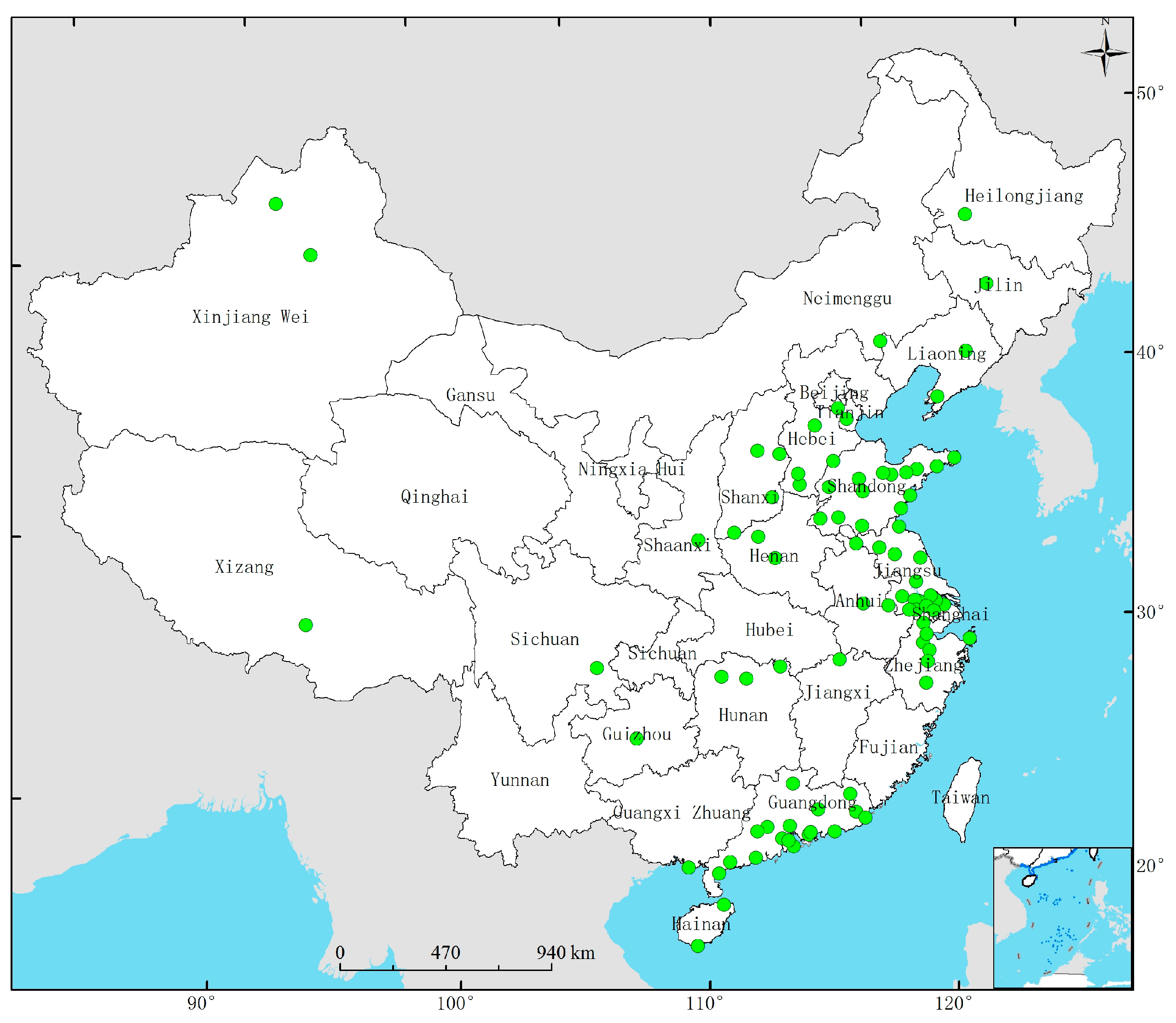
2.3. Ground-Level In Situ Measurement

Along with the rapid economic growth that has occurred over the past two decades, environmental pollution has emerged as a severe issue in China. The Chinese government has established the China National Environmental Monitoring Centre (CNEMC), which is directly affiliated with the ministry of environmental protection of the People’s Republic of China. CNEMC’s main functions are to undertake state environmental monitoring, develop state environmental monitoring technologies, and provide monitoring information and technical support to the country’s environmental management and decision-making bodies. Since the beginning of 2013, CNEMC has begun to establish a network for monitoring ground-level NO2 concentrations over China. Currently, there are more than 800 atmospheric pollution-monitoring stations in this network, hourly ground-level NO2 concentrations released by these monitoring stations were measured with the standard methods (http://www.cnemc.cn/publish/totalWebSite/0493/187/newList_1.html). The Thermo Scientific Model 42i, which is used to monitor ground-level NO2 concentrations in these monitoring stations, is designated by the United States Environmental Protection Agency (US EPA) as a Reference Method for the measurement of ambient concentrations of NO2 pursuant with the requirements defined in the Code of Federal Regulations. The Model 42i Chemiluminescence Analyzer combines proven detection technology, easy-to-use menu-driven software, and advanced diagnostics to offer unsurpassed flexibility and reliability. We found that the 2014 annual observation data is the most abundant, and has the minimum discontinuity after statistics.
In this study, we used ground-level NO2 concentration observation data released by CNEMC-monitored stations in 2014 to compare. We first eliminated the data released by the CNEMC stations that had a monitoring time of less than 20 days a month. Then, we analyzed the longitude and latitude of each monitored station, computed the mean of the data released by stations distributed in the same 64 km grid cell according to latitude and longitude. In addition, because the OMI was launched into a Sun-synchronous orbit crossing the equator at approximately 13:45, we computed the mean of the CNEMC’s ground-level NO2 concentration observation data between 13:00 and 14:00 as daily mean values to compare. In this study we obtained monthly mean values of ground-level NO2 concentrations released by 100 CNEMC monitored stations. Distribution of these 100 monitored stations is shown in Figure 2.

2.4. Determination of Ground-Level NO2 Concentrations

Airborne measurements of the southeastern United States show that NO2 in the boundary layer can greatly contribute to NO2 tropospheric columns over polluted regions [54]. Retrievals based on satellite observations have revealed a close relationship between land surface NO2 emissions and tropospheric NO2 columns [36,55,56,57,58,59]. These studies clearly suggest that tropospheric NO2 columns retrieved from satellite observations can be used to derive the ground-level NO2 concentrations. In this study, we used the RAMS-CMAQ modeling system to simulate the relationship between satellite observations of tropospheric NO2 columns and the ground-level NO2 concentrations over China following the method described by Lamsal et al. [60,61], who conducted a simulation of tropospheric NO2 profiles over the United States and Canada using the Goddard Earth Observing System (GEOS)-Chem global three-dimensional model of tropospheric chemistry at 2° × 2.5°, version 7-03-06. However, previous research on ground-level NO2 concentrations by combining with satellite observations and model simulations has failed to consider the influence of China’s high atmospheric pollution on obtaining the vertical distribution of tropospheric NO2 profiles over China. In addition, compared to the GEOS-Chem global model, the RAMS-CMAQ modeling system, with its higher spatial resolution of a 64 km grid cell, is more appropriate to simulating tropospheric NO2 profiles over China. Many works have shown that the modeled NO2 concentrations over China by the RAMS-CMAQ modeling system are more appropriately suited to China’s high atmospheric pollution [51,52,53]. In this study we compensated for this shortcoming by estimating ground-level NO2 concentrations over China using the OMI standard NO2 product combined with simulations from the RAMS-CMAQ model, after obtaining the more appropriate vertical distribution of tropospheric NO2 profiles.
In this study, the different spatial resolution from the OMI standard NO2 product and simulation from the RAMS-CMAQ modeling system has hindered the estimating of ground-level NO2 concentrations over China. Our approach to reconstructing consistent spatial resolution was to degrade higher spatial resolution data to a single consistent coarse spatial resolution. Here we first calculated the distance of latitude and longitude from each grid cell of the RAMS-CMAQ model with relatively coarse spatial resolution of 64 × 64 km2 grid cells to all grid cells of the OMI tropospheric NO2 columns with higher spatial resolution of 13 × 24 km2, and considered the two grid cells of the different data with minimum distance of latitude and longitude to correspond to each other. Then we estimated ground-level NO2 concentrations over China using the OMI standard NO2 product combined with simulation from the RAMS-CMAQ model after reconstructing a consistent spatial resolution of 64 × 64 km2.

3. Results

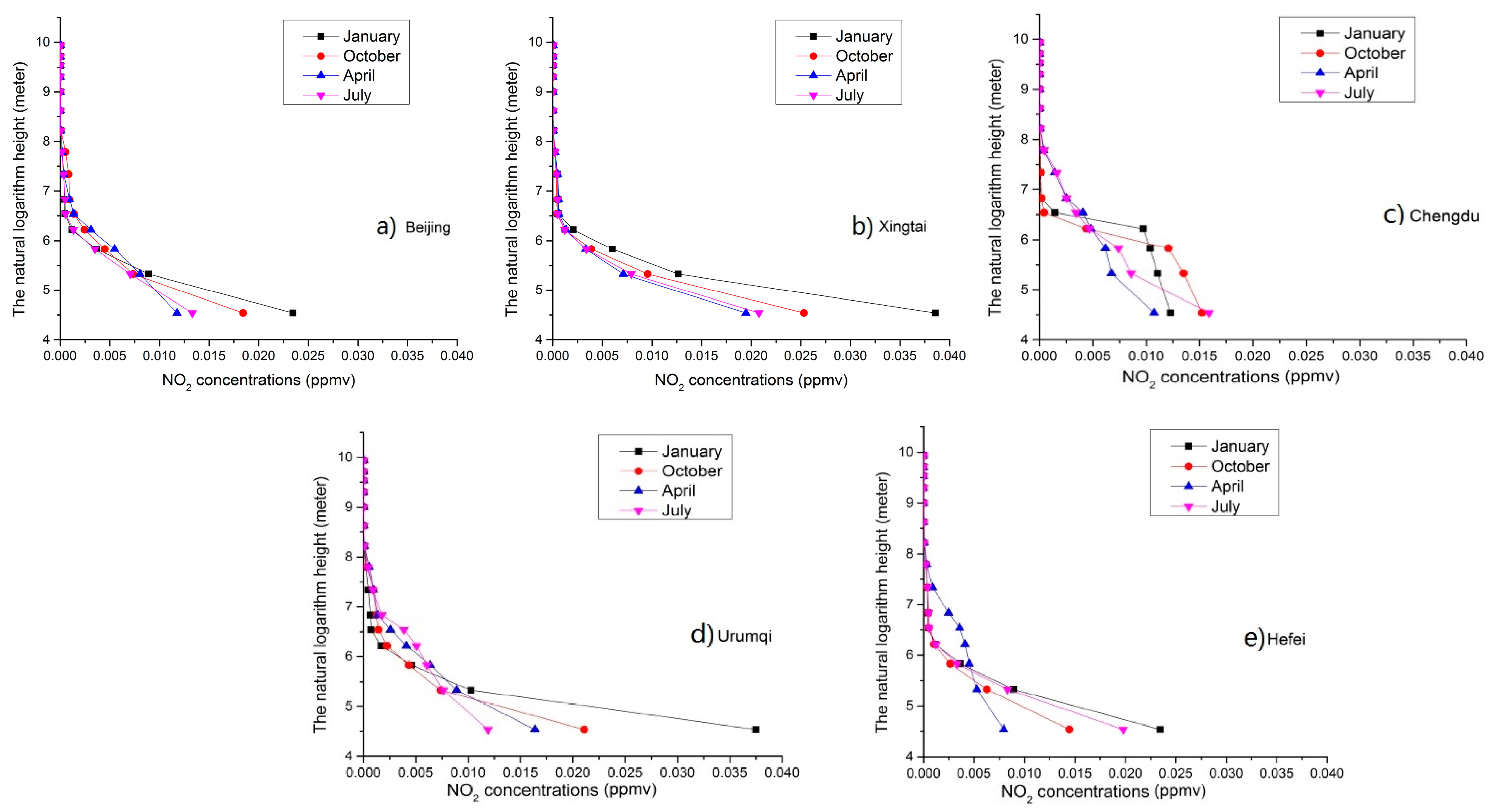
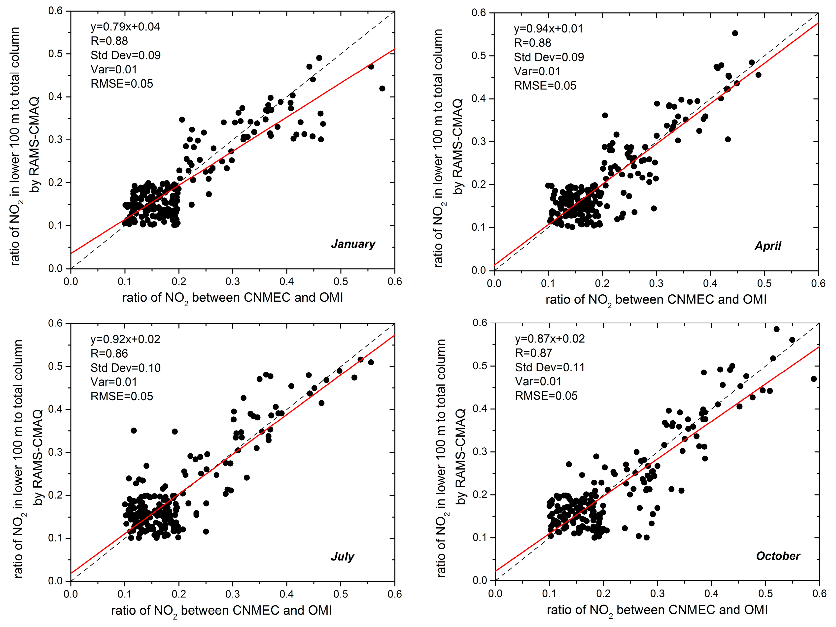
3.1. Verification of Distributions of Tropospheric NO2 Profiles from RAMS-CMAQ

In this section, verification of vertical distributions of tropospheric NO2 profiles from the RAMS-CMAQ model is presented. We first counted the monthly mean of tropospheric NO2 columns from OMI observations over China in 2014. After the corresponding unit conversion, we calculated the ratio of ground-level NO2 concentrations released by CNEMC to tropospheric NO2 columns by OMI, then compared the ratio of simulated NO2 concentrations distributed within the atmosphere from the ground to a height of 100 m to simulated concentrations distributed within the atmosphere from the ground to ~23 km by the RAMS-CMAQ model. We verified the accuracy of the vertical distribution of tropospheric NO2 profiles over China from the RAMS-CMAQ model by comparing the correlation of these two sets of ratios, the results of which are shown in Figure 3.
It is found that the vertical distribution of tropospheric NO2 profiles over China has a large spatial and temporal variation. To illustrate these spatial-temporal variations in tropospheric NO2 profiles over China, we chose to analyze the vertical distributions of tropospheric NO2 profiles in five representative cities: Beijing, Xingtai, Chengdu, Urumqi and Hefei. Information on these five cities is listed in Table 1. The vertical distributions of tropospheric NO2 profiles in these five cities are shown in Figure 4. The x-axis shows NO2 concentrations simulated by the RAMS-CMAQ modeling system, and the y-axis shows the corresponding heights expressed by the natural logarithm. Natural logarithm height was used because the vertical layers by the RAMS-CMAQ modeling system were unequally spaced in the coordinates system, and heights corresponding to the different vertical layers varied dramatically. It is evident from Figure 4 that the tropospheric NO2 columns are mainly distributed within the atmosphere from the ground to a height of 100–150 m.

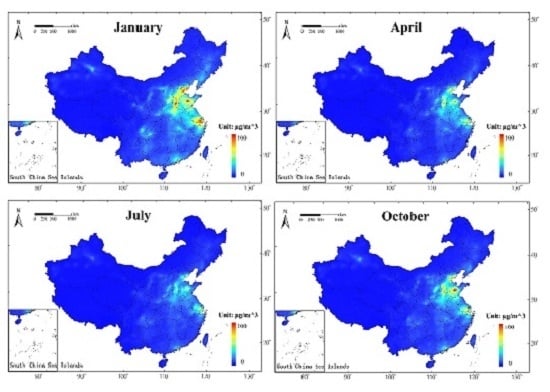
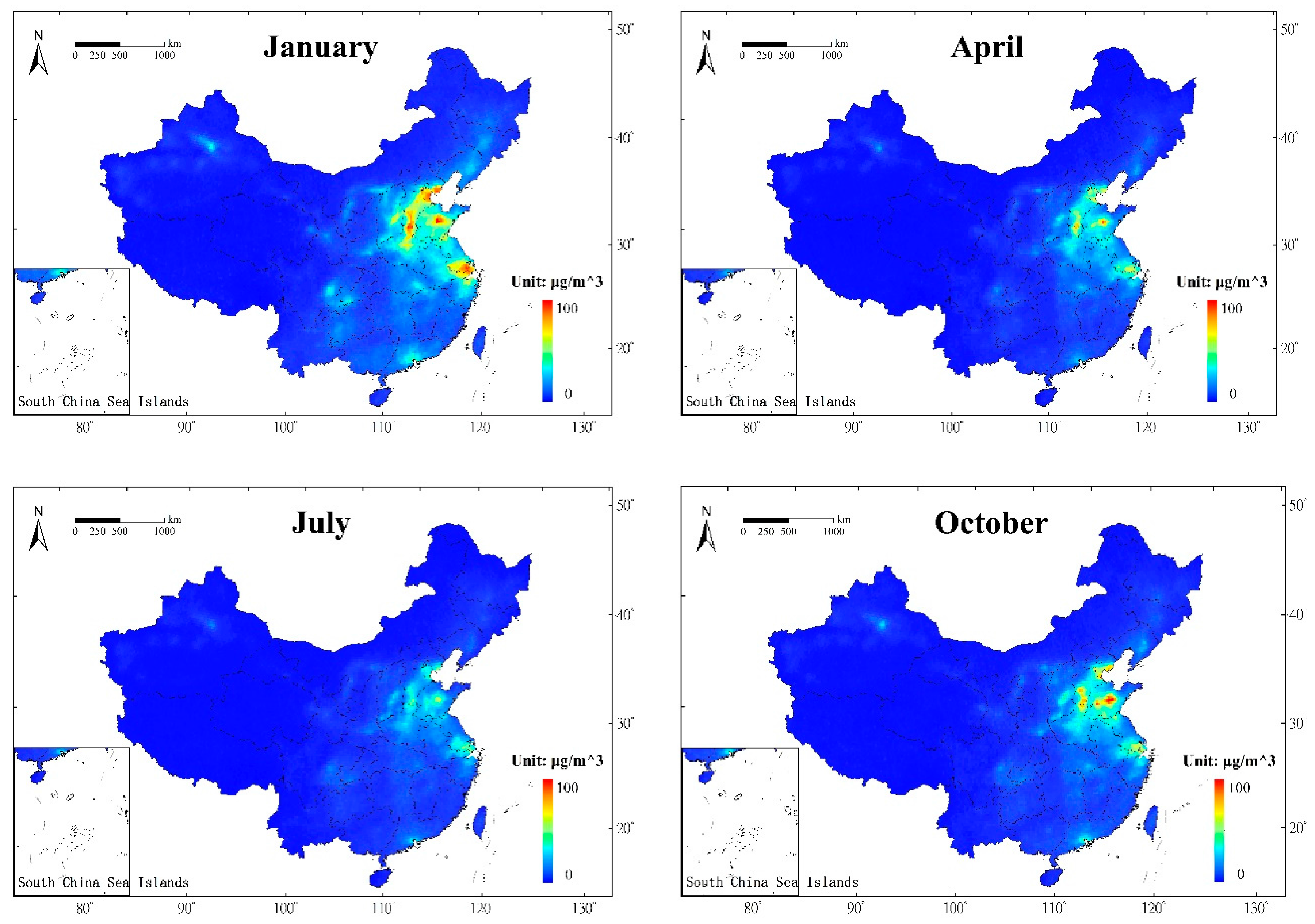
3.2. Spatial-Temporal Variations of Derived Ground-Level NO2 Concentrations

In this section, spatio-temporal variation trends of derived ground-level NO2 concentrations combining OMI observations with the RAMS-CMAQ model are presented. Figure 5 shows the monthly mean values of the derived ground-level NO2 concentrations over China in January, April, July, and October, 2014. From Figure 5, we can see that among different seasons the ground-level NO2 concentration levels over China were high in the winter/spring and low in the summer/fall, and for different regions they were high in the eastern, developed areas, but low in the western, developing areas of China, due to there being more anthropogenic emissions in the eastern areas (e.g., ground-level NO2 concentrations in the developed North China Plain reached 60.00–100.00 μg/m3 whereas concentrations in the less developed western areas reached 5.00–20.00 μg/m3). We analyzed these spatial distribution characteristics of ground-level NO2 concentrations for China in combination with industrial development and anthropogenic emissions. A significant positive correlation was found between the magnitude of ground-level NO2 concentrations and levels of industrial development and anthropogenic emissions. Of the different seasons in China, winter ground-level NO2 concentration values are the highest of the year, which is mainly attributable to winter coal use for heating.

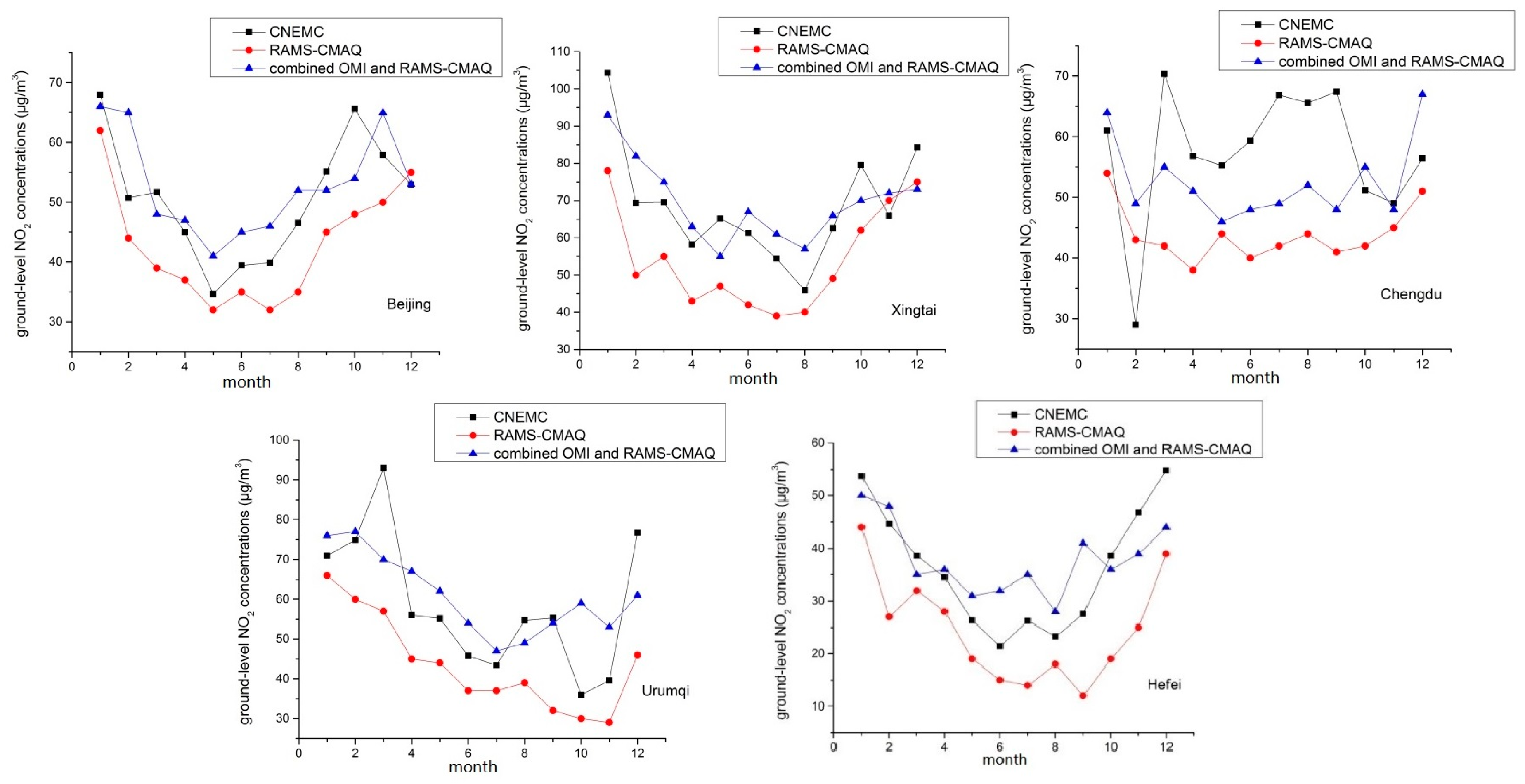
3.3. Comparisons of the Derived NO2 with Ground-Based Measurements for Different Regions

A comparison between monthly mean ground-level NO2 concentrations for different regions from in-situ measurements and the concentrations derived from OMI satellite data in conjunction with the RAMS-CMAQ modeling results is shown in Figure 6, the x-axis is the month, and the y-axis is the ground-level NO2 concentrations. We analyzed the ground-level NO2 concentrations in the five representative cities, i.e., Beijing, Xingtai, Chengdu, Urumqi and Hefei. As the CNEMC atmospheric pollution monitoring stations are unevenly distributed across the country, we first computed the average values of ground-level NO2 concentrations released by all monitoring stations distributed within a city, calculated the average value of OMI tropospheric NO2 columns over the same city, and then we obtained the ground-level NO2 concentrations of the same city. Figure 6 shows that the average correlation coefficients largely fall within a range of 0.70~0.80 for the selected five representative cities of Beijing, Xingtai, Chengdu, Urumqi and Hefei, and that the correlation coefficients for Beijing, Xingtai and Hefei are, relatively, better. Beijing is one of China’s mega cities and has, relatively, more ground monitoring stations. The data quality in Beijing is better, creating a more solid foundation for air pollution monitoring research and long-term monitoring. Xingtai is currently one of the most heavily air-polluted cities in China, and the air quality levels in Xingtai were ranked last. Hefei’s air is similar to Beijing. Figure 6 shows that our method is more precise at determining levels for cities with heavy air pollution, and for those cities with more ground monitoring stations. In general the vertical distributions of tropospheric NO2 profiles for these cities based on the RAMS-CMAQ model are, relatively, more accurate representations of air quality conditions; therefore, ground-level NO2 concentrations retrieved are more accurate.
From Figure 6, we also found that, compared to the in-situ ground measurements, the RAMS-CMAQ simulated values are underestimated, and in areas with high NO2 concentrations, the underestimations are more obvious (e.g., in Xingtai City). Overall, the results of our method are similar to the in-situ measurements. The standard deviation between ground-level NO2 concentrations, the RAMS-CMAQ simulated measurements and those measurements released by CNEMC in Beijing was 10.25 μg/m3, and the standard deviation between our method and CNEMC’s was 9.03 μg/m3. The variance between the RAMS-CMAQ and CNEMC data for Beijing was 105.01, and the variance between our method and that of CNEMC was 81.51. The standard deviation between the RAMS-CMAQ simulated measurements and those released by CNEMC for Xingtai was 15.68 μg/m3, and the standard deviation between our method and that released by CNEMC was 12.65 μg/m3. The variance between the RAMS-CMAQ model and CNEMC results for Xingtai was 246.00, and the variance between our method and that of CNEMC was 160.07. The analysis shows that ground-level NO2 concentrations derived using OMI tropospheric NO2 columns together with vertical distributions of tropospheric NO2 profiles from RAMS-CMAQ model simulations were more accurate than the simulations from RAMS-CMAQ model only.
Figure 6 shows the derived ground-level NO2 concentrations by OMI and RAMS-CMAQ model are generally lower than the in-situ ground measurements by CNEMC in these cities in winter, except for Chengdu, this result is similar to Lamsal’s result that the derived surface NO2 by OMI and GEOS-chem over western North America are generally lower than the local in-situ measurements in winter [60]. Larger differences between the in-situ measurements and the derived ground-level NO2 concentrations in China likely reflect a combination of enhanced spatial variations in polluted regions and preferential placement of in-situ monitors in polluted locations. The ground-level NO2 concentrations estimated from our approach are generally consistent with the in-situ ground measurements for these five cities, and the occasional large discrepancies may reflect local variation processes. In addition, the consumption of bulk coal and household coal for heating, cooking and other uses in winter is common in China, especially in rural areas. However, information about these sources of NO2 emissions are generally not grasped by the government. The emission inventory by the RAMS-CMAQ model generally also overlooks wintertime NO2 emission caused by bulk coal and household coal in China, which led to the underestimation of the derived ground-level NO2 concentrations in winter from our approach. The vertical distribution of tropospheric NO2 profiles over China from the RAMS-CMAQ model as shown in Figure 3 also verified this underestimation of our results. Chengdu is surrounded by mountains. From west to east, the terrain of Chengdu is divided into three parts, comprising mountains, plains and hills. It is difficult to operate the local in-situ NO2 measurements such as the elevation of the western part of Chengdu is mainly over 3 km while the elevation of the central part is about 400 m to 700 m. However, in order to ensure the integrity of this study, it is necessary to study ground-level NO2 concentration in Chengdu, which is a representative metropolis in Southwest China. Meanwhile, the worse result in Chengdu reflects that our approach has to be improved when considering complicated topographies, which is a future work we will conduct. Additionally, more ground-based monitoring data will be helpful for future analysis.

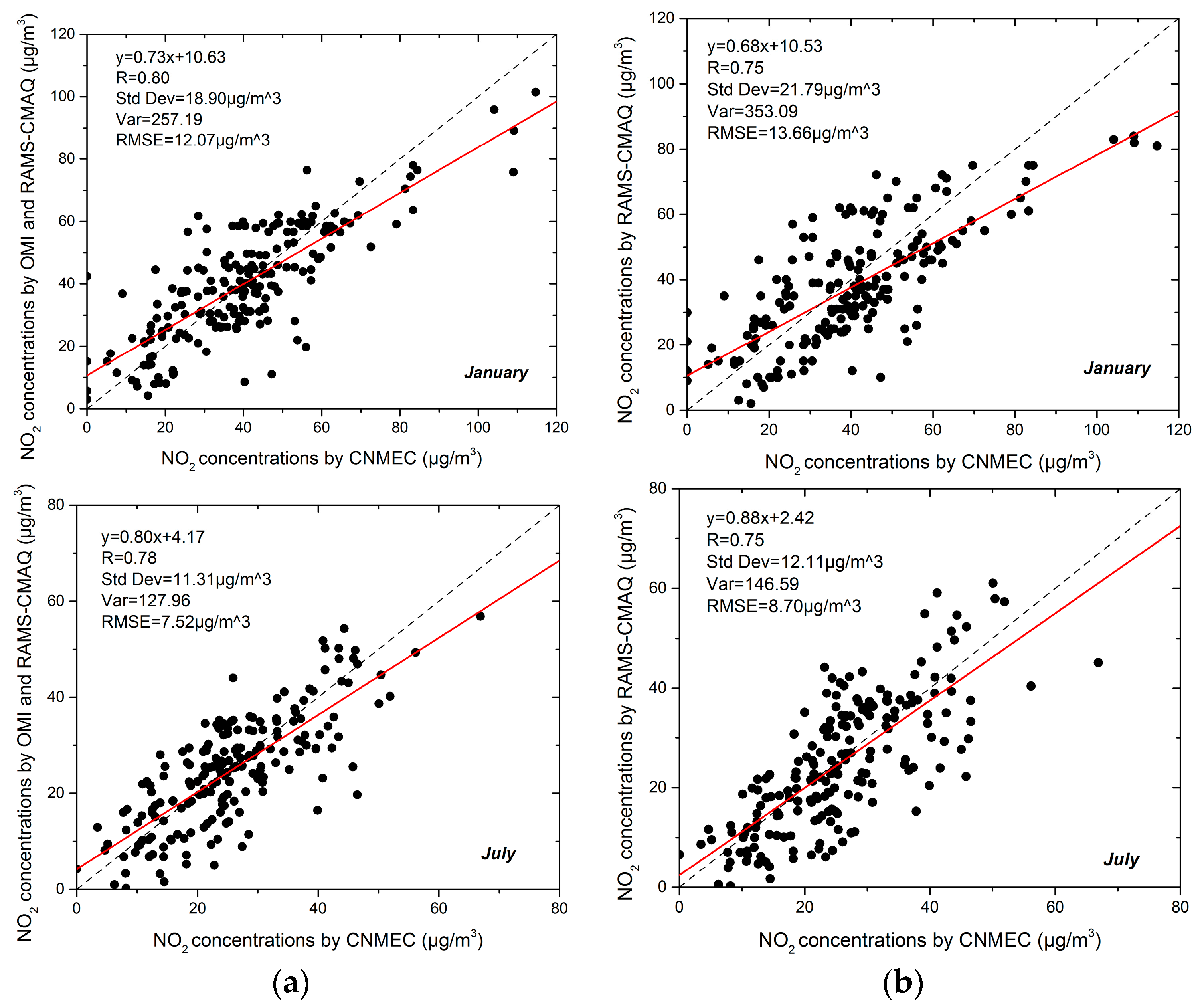
3.4. Comparisons of the Derived NO2 with Ground-Based Measurements for Different Seasons

In this section, we compared the ground-level NO2 concentrations retrieved from our method with in-situ measurements for different seasons across China. As satellite data offer broader observational data coverage than in-situ measurements, data in a large area of China and for different seasons were used. We used mean monthly values from the 100 ground-level NO2 concentration CNEMC-monitored stations mentioned in Section 2.3 to compare. Figure 7 shows good correlations between the derived ground-level NO2 concentrations and the monthly mean ground-level NO2 over China for 2014. The correlation coefficient, R, was 0.80 for January and was 0.78 for July; compared to ground-level NO2 concentrations simulated using the RAMS-CMAQ model only. The standard deviation between our method and those measurements released by CNEMC for January was 18.90 μg/m3, and the standard deviation between the RAMS-CMAQ simulated measurements and CNEMC’s was 21.79 μg/m3. The variance between our method and that released by CNEMC for January was 257.19, and the variance between the RAMS-CMAQ and CNEMC data was 353.09. The standard deviation between our method and that released by CNEMC for July was 11.31 μg/m3, and the standard deviation between the RAMS-CMAQ simulated concentrations and CNEMC’s was 12.11 μg/m3. The variance between our method and that released by CNEMC for July was 127.96, and the variance between the RAMS-CMAQ and CNEMC data was 146.59. Analyzing the ground-level NO2 concentrations retrieved from our method for different seasons, we found clear seasonal variations in the derived ground-level NO2 concentrations, with the largest variations occurring in the winter and the least pronounced in the summer. This is mainly attributable to increases in burning and heating emissions in the winter. Therefore, anthropogenic emission is the main factor that is impacting changes in ground-level NO2 concentrations. The ground-level NO2 concentrations calculated in this paper can be used to measure the influence of anthropogenic emissions on atmospheric quality.
Figure 7 also shows that the ground-level NO2 concentrations estimated by OMI and RAMS-CMAQ model are generally lower than the in-situ measurements by CNEMC over China in January and July, the underestimation of the derived ground-level NO2 concentrations in January from our approach may be caused by the wintertime consumption of bulk coal and household coal in China, which are not considered in the emission inventory by the RAMS-CMAQ model. The underestimation level of the derived ground-level NO2 concentrations in July is lower than in January, which corresponds to the underestimation level of the vertical distributions of tropospheric NO2 profiles as shown in Figure 3. OMI-derived ground-level NO2 concentration represents the mean concentration over several hundred square kilometers, while in-situ measurements are point observations in general, which led to a slope of linear regression line of less than 1 in Figure 7. Possible explanations for the seasonal discrepancy between the derived ground-level NO2 concentrations and in-situ measurements include errors in the in-situ NO2 concentrations, in the RMAS-CMAQ simulated vertical distributions of tropospheric NO2 profiles, and in the OMI tropospheric NO2 column retrieval. Another likely contributor to the seasonal discrepancy is the use of mean NO2 profiles in the OMI air mass factor calculation [60]. Seasonal variation would yield an underestimate in retrieved NO2 columns in winter versus in summer. In addition, seasonal variation in surface reflectivity could also play a part.

4. Discussion

In this study, we have used the OMI tropospheric NO2 columns and the RAMS-CMAQ modeling system to infer ground-level NO2 concentrations. Several previous studies reported that the simulation of tropospheric NO2 profiles over the United States and Canada using the GEOS-Chem global three-dimensional model of tropospheric chemistry at 2° × 2.5° were obtained, and ground-level NO2 concentrations over the United States and Canada were measured by the Ozone Monitoring Instrument (OMI) [60,61]. However, these previous studies on ground-level NO2 concentrations by combining satellite observations and model simulations, on the one hand, has not been implemented in China, and the influence of severe atmospheric pollution also increases the level of difficulty of obtaining the vertical distribution of tropospheric NO2 profiles over China. On the other hand, compared to the GEOS-Chem global model used in the previous studies, the RAMS-CMAQ modeling system with the higher spatial resolution of 64 km grid cell is more appropriate for simulating tropospheric NO2 profiles over China. Much research has shown that the modeled NO2 concentrations over China by the RAMS-CMAQ model are more appropriate to China’s high atmospheric pollution [51,52,53]. In this study we inferred the ground-level NO2 concentrations over China using the OMI NO2 product combined with simulation from the RAMS-CMAQ model after obtaining the more appropriately vertical distribution of tropospheric NO2 profiles.
We derived the ground-level NO2 concentrations using the total column of NO2 observed from the OMI and the simulations from the RAMS-CMAQ model in China. Data for 2014 were processed and compared to in-situ measurements derived from the CNEMC monitoring network. The derived ground-level NO2 concentrations were also compared with the simulated ground-level NO2 concentrations by the RAMS-CMAQ. Overall, ground level NO2 concentrations were underestimated by the RAMS-CMAQ model. Using observed data corresponding to in-situ CNEMC measurements, the standard deviation between the RAMS-CMAQ simulated measurements and in-situ measurements by CNEMC for January was 21.79 μg/m3, it was improved to 18.90 μg/m3 between our method and CNEMC data. The variance between our method and that released by CNEMC for January was 257.19, and the variance between the RAMS-CMAQ and CNEMC data was 353.09, the root mean square error between the RAMS-CMAQ simulations and in-situ measurements by CNEMC for January was 13.66 μg/m3, which was improved to 12.07 μg/m3 between our method and CNEMC data. The standard deviation between the RAMS-CMAQ and CNEMC data for July was 12.11 μg/m3, and it was improved to 11.31 μg/m3 between our method and CNEMC data. The variance between our method and that released by CNEMC for July was 127.96, and the variance between the RAMS-CMAQ data and CNEMC data was 146.59. The root mean square error between the RAMS-CMAQ simulations and in-situ measurements by CNEMC for July was 8.70 μg/m3, which was improved to 7.52 μg/m3 between our method and CNEMC data. Correlation coefficients between the RAMS-CMAQ simulation and in-situ measurements were 0.75 for January and July, and they were improved to 0.80 and 0.78, respectively, from our approach. Compared to that of the in-situ measurements in different regions, the standard deviation between ground-level NO2 concentrations, the RAMS-CMAQ simulated measurements, and in-situ measurements released by CNEMC in Beijing was 10.25 μg/m3, which was improved to 9.03 μg/m3 between our method and CNEMC data33; the standard deviation between the RAMS-CMAQ and CNEMC data in Xingtai was 15.68 μg/m3, which was improved to 12.65 μg/m3 between our method and CNEMC data.
Major errors in the retrieval of ground-level NO2 concentrations using the total column of NO2 observed from the OMI and the simulations from the RAMS-CMAQ model have been estimated in the following aspects. First, the errors in the retrieval of OMI tropospheric NO2 columns have been estimated at ~0.7 × 10¹⁵ mol cm−2 from the slant column fitting (~0.15 × 10¹⁵ mol cm−2 in the stratospheric slant column and ~0.5 × 10¹⁵–1.5 × 10¹⁵ mol cm−2 in the tropospheric AMF for individual cloud-free pixels (with an effective cloud fraction of <0.2)) [31]. AMF errors are mainly from cloud interference, surface albedo, aerosol, and profile shape uncertainties [29,30,32,36,37]. Separation between the stratosphere and troposphere is also a source of error; and while the overall error in the OMI vertical NO2 columns under clear and unpolluted conditions is estimated at 5%, it can reach up to 50% in the presence of pollution and clouds [32]. Second, in this study, we used the RAMS-CMAQ modeling system to simulate of tropospheric NO2 profiles over China. The emission inventory by the RAMS-CMAQ model, such as the anthropogenic emissions of aerosols and their precursors (CO, NOx, SO2, volatile organic compounds (VOCs), black carbon, and organic carbon, PM2.5, and PM10), are obtained from the monthly emission inventory [46,47,48] updated from the previous version [49] over East Asia. The errors in the retrieval of tropospheric NO2 profiles over China by the RAMS-CMAQ model are mainly due to the emission inventory and the meteorology field. The meteorology field is important to the modeled mass concentrations, aerosols and their precursor simulations. The accuracy of wind field and relative humidity simulation could obviously affect the dust particle transport and optical properties calculation [50]. Last, because the different spatial resolution from the OMI standard NO2 product and simulation from the RAMS-CMAQ model has hindered the estimating ground-level NO2 concentrations, another source of error was the reconstructed consistent spatial resolution, for which we degraded the higher spatial resolution data to a single consistent coarse spatial resolution.
In this study, we did not take into account the averaging kernel (AK). AK is a well-established concept in the retrieval of remote sensing observations as the link between the retrieved quantities and reality. It is proportional to the height-dependent sensitivity of satellite observation to changes in tracer concentration, and provides the interpretation of the value of the air mass factor. The AK provides important information needed for quantitative analysis of the satellite data, especially for interpreting the satellite retrieval of trace gases to users. It’s very useful to remove the dependence on a priori assumptions about the profile shape for inter-comparison between model simulations and satellite measurements. In this paper, we focused on estimating ground-level NO2 by combining the OMI standard product OMNO2 from NASA (Version 3) and the RAMS-CMAQ modeled NO2 profiles, rather than on satellite-model comparison, so we didn’t consider the AK in this study. However, the OMI NO2 standard product is not directly suitable to studying VCDs on a scale below the resolution of the ancillary parameters (such as 2° × 2.5° for priori NO2 profiles), and the AK can be used to correct the NO2 VCDs when more accurate NO2 profiles are available, which will improve satellite NO2 VCD products and also the ground-level nitrogen dioxide concentrations inferred from satellites. While this correction is beyond the scope of this study, we are developing a customized OMI NO2 retrieval by recalculating AKs using the high-resolution RAMS-CMAQ modeled NO2 profiles, and will apply it to the estimation of ground-level NO2 in future study. We did not take into account NO2 emissions from natural sources such as biomass burning, soil, and lightning, because they are negligible compared to anthropogenic emissions over urban areas. In addition, the contribution of free tropospheric NO2 produced from lightning mainly occur in low latitude areas, while the NO2 high concentration areas, such as the Beijing Tianjin Hebei region, were mainly distributed in the middle and high latitude areas.

5. Conclusions

Most works using satellite observations of NO2 focused on tropospheric NO2 columns rather than on ground-level NO2 concentrations. However, ground-level NO2 concentrations are more closely related to anthropogenic emissions and directly affect human health. This paper presents a means of estimating ground-level NO2 concentrations based on OMI tropospheric NO2 columns and the vertical distribution of tropospheric NO2 profiles simulated using the RAMS-CMAQ model. One year’s worth of data from 2014 was processed and the results were compared to ground-based NO2 measurements from a network of CNEMC, and the simulated ground-level NO2 concentrations by the RAMS-CMAQ model. Our results revealed that the method presented in this paper can be used to better measure ground-level NO2 concentrations over China.
Further analysis of the ground-level NO2 concentrations retrieved from this algorithm shows that seasonal variations of the ground-level NO2 concentrations are pronounced, with the largest occurring in the winter and the lowest in the summer. Such variations are mainly due to significant increases in burning and heating emissions levels in winter. The ground-level NO2 concentrations presented in this paper can be used to better measure distribution of NO2 in the atmosphere and study the effects of anthropogenic emissions on atmospheric pollution conditions. Further validations and improvements of this method are ongoing, and include the quality control of in-situ measurements, whose errors have not been taken into account. We plan to develop a simple empirical formula based on the CMAQ model for directly converting OMI column values to ground-level NO2. Such an algorithm may be used to more accurately monitor ground-level NO2 using satellite data and to generate measurements with better spatial and temporal coverage than surface measurements.

Acknowledgments

This work was supported by the National Natural Science Foundation of China (Grant No. 41501476) and the National Science and Technology Ministry (Grant No. 2014BAC21B03), this work was partially supported by China Postdoctoral Science Foundation funded project (Grant No. 2015M580084, 2016T90083). We greatly acknowledge the free use of tropospheric NO2 column data from the OMI sensor. We also thank State Key Laboratory of Atmospheric Boundary Layer Physics and Atmospheric Chemistry, Chinese Academy of Sciences for the RAMS-CMAQ simulation data. We also thank China’s National Environmental Monitoring Centre for in-situ measurements.

Author Contributions

The authors contributed equally to the manuscript.

Conflicts of Interest

The authors declare no conflict of interest.

References

  1. Logan, J.A. Nitrogen Oxides in the Troposphere: Global and Regional Budgets. J. Geophys. Res. 1983, 88, 10785–10807. [Google Scholar] [CrossRef]
  2. Finlayson-Pitts, F.C.; Pitts, J.N., Jr. (Eds.) Atmospheric Chemistry: Fundamentals and Experimental Techniques; John Wiley: Hoboken, NJ, USA, 1986. [Google Scholar]
  3. Solomon, S.; Portmann, R.W.; Sanders, R.W.; Daniel, J.S.; Madsen, W.; Bartram, B.; Dutton, E.G. On the Role of Nitrogen Dioxide in the Absorption of Solar Radiation. J. Geophys. Res. 1999, 1041, 12047–12058. [Google Scholar] [CrossRef]
  4. Crutzen, P.J. The Role of NO and NO2 in the Chemistry of the Troposphere and Stratosphere. Annu. Rev. Earth Planet. Sci. 1979, 7, 443–472. [Google Scholar] [CrossRef]
  5. Sunyer, J.; Spix, C.; Quénel, P.; Ponce-de-León, A.; Pönka, A.; Barumandzadeh, T.; Touloumi, G.; Bacharova, L.; Wojtyniak, B.; Vonk, J.; et al. Urban Air Pollution and Emergency Admissions for Asthma in Four European Cities: the APHEA Project. Thorax 1997, 52, 760–765. [Google Scholar] [CrossRef] [PubMed]
  6. Latza, U.; Gerdes, S.; Baur, X. Effects of Nitrogen Dioxide on Human Health: Systematic Review of Experimental and Epidemiological Studies Conducted between 2002 and 2006. Int. J. Hyg. Environ. Health 2009, 212, 271–287. [Google Scholar] [CrossRef] [PubMed]
  7. Chen, R.; Samoli, E.; Wong, C.M.; Huang, W.; Wang, Z.; Chen, B.; Kan, H. CAPES Collaborative Group. Associations between Short-Term Exposure to Nitrogen Dioxide and Mortality in 17 Chinese Cities: the China Air Pollution and Health Effects Study (CAPES). Environ. Int. 2012, 45, 32–38. [Google Scholar] [CrossRef] [PubMed]
  8. Ackermann-Liebrich, U.; Leuenberger, P.; Schwartz, J.; Schindler, C.; Monn, C.; Bolognini, G.; Bongard, J.P.; Brändli, O.; Domenighetti, G.; Elsasser, S.; et al. Lung Function and Long Term Exposure to Air Pollutants in Switzerland. Study on Air Pollution and Lung Diseases in Adults (SAPALDIA) Team. Am. J. Respir. Crit. Care Med. 1997, 155, 122–129. [Google Scholar] [CrossRef] [PubMed]
  9. Schindler, C.; Ackermann-Liebrich, U.; Leuenberger, P.; Monn, C.; Rapp, R.; Bolognini, G.; Bongard, J.P.; Brändli, O.; Domenighetti, G.; Karrer, W.; et al. Associations between Lung Function and Estimated Average Exposure to NO2 in Eight Areas of Switzerland. The SAPALDIA Team. Swiss Study of Air Pollution and Lung Diseases in Adults. Epidemiology 1998, 9, 405–411. [Google Scholar] [CrossRef] [PubMed]
  10. Panella, M.; Tommasini, V.; Binotti, M.; Palin, L.; Bona, G. Monitoring Nitrogen Dioxide and Its Effects on Asthmatic Patients: Two Different Strategies Compared. Environ. Monit. Assess. 2000, 63, 447–458. [Google Scholar] [CrossRef]
  11. Smith, B.J.; Nitschke, M.; Pilotto, L.S.; Ruffin, R.E.; Pisaniello, D.L.; Willson, K.J. Health Effects of Daily Indoor Nitrogen Dioxide Exposure in People with Asthma. Eur. Respir. J. 2000, 16, 879–885. [Google Scholar] [CrossRef] [PubMed]
  12. Gauderman, W.J.; McConnell, R.; Gilliland, F.; London, S.; Thomas, D.; Avol, E.; Vora, H.; Berhane, K.; Rappaport, E.B.; Lurmann, F.; et al. Association between Air Pollution and Lung Function Growth in Southern California Children. Am. J. Respir. Crit. Care Med. 2000, 162, 1383–1390. [Google Scholar] [CrossRef] [PubMed]
  13. Gauderman, W.J.; Gilliland, G.F.; Vora, H.; Avol, E.; Stram, D.; McConnell, R.; Thomas, D.; Lurmann, F.; Margolis, H.G.; Rappaport, E.B.; et al. Association between Air Pollution and Lung Function Growth in Southern California Children: Results from a Second Cohort. Am. J. Respir. Crit. Care Med. 2002, 166, 76–84. [Google Scholar] [CrossRef] [PubMed]
  14. Stieb, D.M.; Judek, S.; Burnett, R.T. Meta-Analysis of Time-Series Studies of Air Pollution and Mortality: Update in Relation to the Use of Generalized Additive Models. J. Air Waste Manag. Assoc. 2003, 53, 258–261. [Google Scholar] [CrossRef] [PubMed]
  15. Burnett, R.T.; Stieb, D.; Brook, J.R.; Cakmak, S.; Dales, R.; Raizenne, M.; Vincent, R.; Dann, T. The Short-Term Effects of Nitrogen Dioxide on Mortality in Canadian Cities. Arch. Environ. Health 2004, 59, 228–237. [Google Scholar] [CrossRef] [PubMed]
  16. Samoli, E.; Aga, E.; Touloumi, G.; Nisiotis, K.; Forsberg, B.; Lefranc, A.; Pekkanen, J.; Wojtyniak, B.; Schindler, C.; Niciu, E.; et al. Short Term Effects of Nitrogen Dioxide and Mortality: An Analysis within the APHEA Project. Eur. Respir. J. 2006, 27, 1129–1137. [Google Scholar] [CrossRef] [PubMed]
  17. Schaap, M.; Müller, K.; ten Brink, H.M. Constructing the European Aerosol Nitrate Concentration Field from Quality Analysed Data. Atmos. Environ. 2002, 36, 1323–1335. [Google Scholar] [CrossRef]
  18. Tørseth, K.; Aas, W.; Breivik, K.; Fjæraa, A.M.; Fiebig, M.; Hjellbrekke, A.G.; Lund Myhre, C.; Solberg, S.; Yttri, K.E. Introduction to the European Monitoring and Evaluation Programme (EMEP) and Observed Atmospheric Composition Change During 1972–2009. Atmos. Chem. Phys. 2012, 12, 5447–5481. [Google Scholar] [CrossRef]
  19. Zhou, Y.; Brunner, D.; Hueglin, C.; Henne, S.; Staehelin, J. Changes in OMI Tropospheric NO2 Columns over Europe from 2004 to 2009 and the Influence of Meteorological Variability. Atmos. Environ. 2012, 46, 482–495. [Google Scholar] [CrossRef]
  20. Castellanos, P.; Boersma, K.F. Reductions in Nitrogen Oxides over Europe Driven by Environmental Policy and Economic Recession. Sci. Rep. 2012, 2, 265. [Google Scholar] [CrossRef] [PubMed]
  21. Hilboll, A.; Richter, A.; Burrows, J.P. Long-Term Changes of Tropospheric NO2 over Megacities Derived from Multiple Satellite Instruments. Atmos. Chem. Phys. 2013, 13, 4145–4169. [Google Scholar] [CrossRef]
  22. Curier, R.L.; Kranenburg, R.; Segers, A.J.S.; Timmermans, R.M.A.; Schaap, M. Synergistic Use of OMI NO2 Tropospheric Columns and LOTOS-EUROS to Evaluate the NOx Emission Trends across Europe. Remote Sens. Environ. 2014, 149, 58–69. [Google Scholar] [CrossRef]
  23. Burrows, J.P.; Weber, M.; Buchwitz, M.; Rozanov, V.; Ladstätter-Weißenmayer, A.; Richter, A.; DeBeek, R.; Hoogen, R.; Bramstedt, K.; Eichmann, K.; et al. The Global Ozone Monitoring Experiment (GOME): Mission Concept and First Scientific Results. J. Atmos. Sci. 1999, 56, 151–175. [Google Scholar] [CrossRef]
  24. Bovensmann, H.; Burrows, J.P.; Buchwitz, M.; Frerick, J.; Noël, S.; Rozanov, V.V.; Chance, K.V.; Goede, A.P.H. SCIAMACHY: Mission Objectives and Measurement Modes. J. Atmos. Sci. 1999, 56, 127–150. [Google Scholar] [CrossRef]
  25. Levelt, P.F.; Hilsenrath, E.; Leppelmeier, G.W.; van den Oord, G.H.J.; Bhartia, P.K.; Tamminen, J.; de Haan, J.F.; Veefkind, J.P. Science Objectives of the Ozone Monitoring Instrument. IEEE Trans. Geosci. Remote Sens. 2006, 44, 1199–1208. [Google Scholar] [CrossRef]
  26. Levelt, P.F.; van den Oord, G.H.J.; Dobber, M.R.; Malkki, A.; Visser, H.; de Vries, J.; Stammes, P.; Lundell, J.O.V.; Saari, H. The Ozone Monitoring Instrument. IEEE Trans. Geosci. Remote Sens. 2006, 44, 1093–1101. [Google Scholar] [CrossRef]
  27. Callies, J.; Corpaccioli, E.; Eisinger, M.; Hahne, A.; Lefebvre, A. GOME-2, Metop’s Second Generation Sensor for Operational Ozone Monitoring. ESA Bull. 2000, 102, 28–36. [Google Scholar]
  28. Richter, A.; Burrows, J.P. Retrieval of Tropospheric NO2 from GOME Measurements. Adv. Space Res. 2002, 29, 1673–1683. [Google Scholar] [CrossRef]
  29. Martin, R.V.; Chance, K.; Jacob, D.J.; Kurosu, T.P.; Spurr, R.J.D.; Bucsela, E.; Gleason, J.F.; Palmer, P.I.; Bey, I.; Fiore, A.M.; et al. An Improved Retrieval of Tropospheric Nitrogen Dioxide from GOME. J. Geophys. Res. 2002, 107, 4437. [Google Scholar] [CrossRef]
  30. Boersma, K.F.; Eskes, H.J.; Brinksma, E.J. Error Analysis for Tropospheric NO2 Retrieval from Space. J. Geophys. Res. 2004, 109, D04311. [Google Scholar] [CrossRef]
  31. Boersma, K.F.; Eskes, H.J.; Veefkind, J.P.; Brinksma, E.J.; van der A, R.J.; Sneep, M.; van den Oord, G.H.J.; Levelt, P.; Stammes, P.; Gleason, J.F.; et al. Near-Real Time Retrieval of Tropospheric NO2 from OMI. Atmos. Chem. Phys. 2007, 7, 2103–2118. [Google Scholar] [CrossRef]
  32. Boersma, K.F.; Bucsela, E.J.; Brinksma, E.J.; Gleason, J.F. NO2. In OMI Algorithm Theoretical Basis Document, OMI Trace Gas Algorithms; ATB-OMI-04, Version 2.0; Chance, K., Ed.; NASA Distributed Active Archive Centers: Greenbelt, MD, USA, 2002; Volume 4. [Google Scholar]
  33. Bucsela, E.J.; Celarier, E.A.; Wenig, M.O.; Gleason, J.F.; Veefkind, J.P.; Boersma, K.F.; Brinksma, E.J. Algorithm for NO2 Vertical Column Retrieval from the Ozone Monitoring Instrument. IEEE Trans. Geosci. Remote Sens. 2006, 44, 1245–1258. [Google Scholar] [CrossRef]
  34. Celarier, E.A.; Brinksma, E.J.; Gleason, J.F.; Veefkind, J.P.; Cede, A.; Herman, J.R.; Ionov, D.; Goutail, F.; Pommereau, J.; Lambert, J.; et al. Validation of Ozone Monitoring Instrument Nitrogen Dioxide Columns. J. Geophys. Res. 2008, 113, D15S15. [Google Scholar] [CrossRef]
  35. Platt, U. Differential Optical Absorption Spectroscopy (DOAS). In Air Monitoring by Spectroscopic Techniques; Sigrist, M., Ed.; John Wiley: Hoboken, NJ, USA, 1994; pp. 27–84. [Google Scholar]
  36. Martin, R.V.; Jacob, D.J.; Chance, K.; Kurosu, T.P.; Perner, P.I.; Evans, M.J. Global Inventory of Nitrogen Oxide Emission Constrained by Space-Based Observations of NO2 Columns. J. Geophys. Res. 2003, 108, 4537. [Google Scholar] [CrossRef]
  37. Hong, H.; Lee, H.; Kim, J.; Jeong, U.; Ryu, J.; Lee, D.S. Investigation of Simultaneous Effects of Aerosol Properties and Aerosol Peak Height on the Air Mass Factors for Space-Borne NO2 Retrievals. Remote Sens. 2017, 9, 208. [Google Scholar] [CrossRef]
  38. Dobber, M.; Kleipool, Q.; Dirksen, R.; Levelt, P.; Jaross, G.; Taylor, S.; Kelly, T.; Flynn, L.; Leppelmeier, G.; Rozemeijer, N. Validation of Ozone Monitoring Instrument Level 1b Data Products. J. Geophys. Res. 2008, 113, D15S06. [Google Scholar] [CrossRef]
  39. Byun, D.; Schere, K. Review of the governing equations, computation algorithms, and other components of the Models-3 Community Multiscale Air Quality (CMAQ) modeling system. Appl. Mech. Rev. 2006, 59, 51–77. [Google Scholar] [CrossRef]
  40. Byun, D.W.; Ching, J. Science Algorithms of the EPA Models-3 Community Multi-Scale Air Quality (CMAQ) Modeling System; NERL: Research Triangle Park, NC, USA, 1999; p. 425. [Google Scholar]
  41. Sarwar, G.; Luecken, D.; Yarwood, G.; Whitten, G.; Carter, W. Impact of an Updated Carbon Bond Mechanism on Predictions from the CMAQ Modeling System: Preliminary Assessment. J. Appl. Meteorol. Climatol. 2008, 47, 3–14. [Google Scholar] [CrossRef]
  42. Zhang, M.; Uno, I.; Sugata, S.; Wang, Z.; Byun, D.; Akimoto, H. Numerical Study of Boundary Layer Ozone Transport and Photochemical Production in East Asia in the Wintertime. Geophys. Res. Lett. 2002, 29. [Google Scholar] [CrossRef]
  43. Zhang, M. Large-Scale Structure of Trace Gas and Aerosol Distributions over the Western Pacific Ocean During the Transport and Chemical Evolution Over the Pacific (TRACE-P) Experiment. J. Geophys. Res. 2003, 108, 8820. [Google Scholar] [CrossRef]
  44. Zhang, M.G.; Uno, I.; Yoshida, Y.; Xu, Y.; Wang, Z.; Akimoto, H.; Bates, T.; Quinn, T.; Bandy, A.; Blomquist, B. Transport and Transformation of Sulfur Compounds over East Asia during the TRACE-P and ACE-Asia Campaigns. Atmos. Environ. 2004, 38, 6947–6959. [Google Scholar] [CrossRef]
  45. Zhang, M.G. Modeling of Organic Carbon Aerosol Distributions over East Asia in the Springtime. China Part. 2004, 2, 192–195. [Google Scholar] [CrossRef]
  46. Lu, Z.; Streets, D.G.; Zhang, Q.; Wang, S.; Carmichael, G.R.; Cheng, Y.F.; Wei, C.; Chin, M.; Diehl, T.; Tan, Q. Sulfur dioxide emissions in China and sulfur trends in East Asia since. Atmos. Chem. Phys. 2000, 10, 6311–6331. [Google Scholar] [CrossRef]
  47. Lu, Z.; Zhang, Q.; Streets, D.G. Sulfur dioxide and primary carbonaceous aerosol emissions in China and India, 1996–2010. Atmos. Chem. Phys. 2011, 11, 9839–9864. [Google Scholar] [CrossRef]
  48. Lei, Y.; Zhang, Q.; He, K.; Streets, D. Primary anthropogenic aerosol emission trends for China, 1990–2005. Atmos. Chem. Phys. 2011, 11, 931–954. [Google Scholar] [CrossRef]
  49. Zhang, Q.; Streets, D.; Carmichael, G.; He, K.; Huo, H.; Kannari, A.; He, K.; Huo, H.; Kannari, A.; Klimont, Z.; et al. Asian emissions in 2006 for the NASA INTEX-B mission. Atmos. Chem. Phys. 2009, 9, 5131–5153. [Google Scholar] [CrossRef]
  50. Han, X.; Ge, C.; Tao, J.; Zhang, M.; Zhang, R. Air quality modeling for a strong dust event in East Asia in March 2010. Aerosol Air Qual. Res. 2012, 12, 615–628. [Google Scholar] [CrossRef]
  51. Han, X.; Zhang, M.; Tao, J.; Wang, L.; Gao, J.; Wang, S.; Chai, F. Modeling aerosol impacts on atmospheric visibility in Beijing with RAMS-CMAQ. Atmos. Environ. 2013, 72, 177–191. [Google Scholar] [CrossRef]
  52. Han, X.; Zhang, M.; Gao, J.; Wang, S.; Chai, F. Modeling analysis of the seasonal characteristics of haze formation in Beijing. Atmos. Chem. Phys. 2014, 14, 10231–10248. [Google Scholar] [CrossRef]
  53. Han, X.; Zhang, M.; Zhu, L.; Skorokhod, A. Assessment of the impact of emissions reductions on air quality over North China Plain. Atmos. Pollut. Res. 2016, 7, 249–259. [Google Scholar] [CrossRef]
  54. Bucsela, E.J.; Perring, A.E.; Cohen, R.C.; Boersma, K.F.; Celarier, E.A.; Gleason, J.F.; Wenig, M.O.; Bertram, T.H.; Wooldridge, P.J.; Dirksen, R.; et al. Comparison of Tropospheric NO2 In Situ Aircraft Measurements with near-Real-Time and Standard Product Data from the Ozone Monitoring Instrument. J. Geophys. Res. 2008, 113, D16S31. [Google Scholar] [CrossRef]
  55. Leue, C.; Wenig, M.; Wagner, T.; Klimm, O.; Platt, U.; Jähne, B. Quantitative Analysis of NO2 Emissions from Global Ozone Monitoring Experiment Satellite Image Sequences. J. Geophys. Res. 2001, 106, 5493–5505. [Google Scholar] [CrossRef]
  56. Martin, R.V.; Sioris, C.E.; Chance, K.; Ryerson, T.B.; Bertram, T.H.; Wooldridge, P.J.; Cohen, R.C.; Neuman, J.A.; Swanson, A.; Flocke, F.M. Evaluation of Space-Based Constraints on Global Nitrogen Oxide Emissions with Regional Aircraft Measurements over and Downwind of Eastern North America. J. Geophys. Res. 2006, 111. [Google Scholar] [CrossRef]
  57. Jaeglé, L.; Steinberger, L.; Martin, R.V.; Chance, K. Global Partitioning of NOx Sources Using Satellite Observations: Relative Roles of Fossil Fuel Combustion, Biomass Burning and Soil Emissions. Faraday Discuss. 2005, 130, 407–423. [Google Scholar] [CrossRef] [PubMed]
  58. Zhang, Q.; Streets, D.G.; He, K.; Wang, Y.; Richter, A.; Burrows, J.P.; Uno, I.; Jang, C.J.; Chen, D.; Yao, Z.; et al. NOx Emission Trends for China, 1995–2004, The View from the Ground and the View from Space. J. Geophys. Res. 2007, 112, D22306. [Google Scholar] [CrossRef]
  59. Schaap, M.; Kranenburg, R.; Curier, L.; Jozwicka, M.; Dammers, E.; Timmermans, R. Assessing the Sensitivity of the OMI-NO2 Product to Emission Changes across Europe. Remote Sens. 2013, 5, 4187–4208. [Google Scholar] [CrossRef]
  60. Lamsal, L.N.; Martin, R.V.; van Donkelaar, A.; Steinbacher, M.; Celarier, E.A.; Bucsela, E.; Dunlea, E.; Pinto, J.P.; Lamsal, C. Ground-level nitrogen dioxide concentrations inferred from the satellite-borne Ozone Monitoring Instrument. J. Geophys. Res. 2008, 113. [Google Scholar] [CrossRef]
  61. Lamsal, L.N.; Martin, R.V.; van Donkelaar, A.; Celarier, E.A.; Bucsela, E.J.; Boersma, K.F.; Dirksen, R.; Luo, C.; Wang, Y. Indirect validation of tropospheric nitrogen dioxide retrieved from the OMI satellite instrument: insight into the seasonal variation of nitrogen oxides at northern midlatitudes. J. Geophys. Res. 2010, 115. [Google Scholar] [CrossRef]
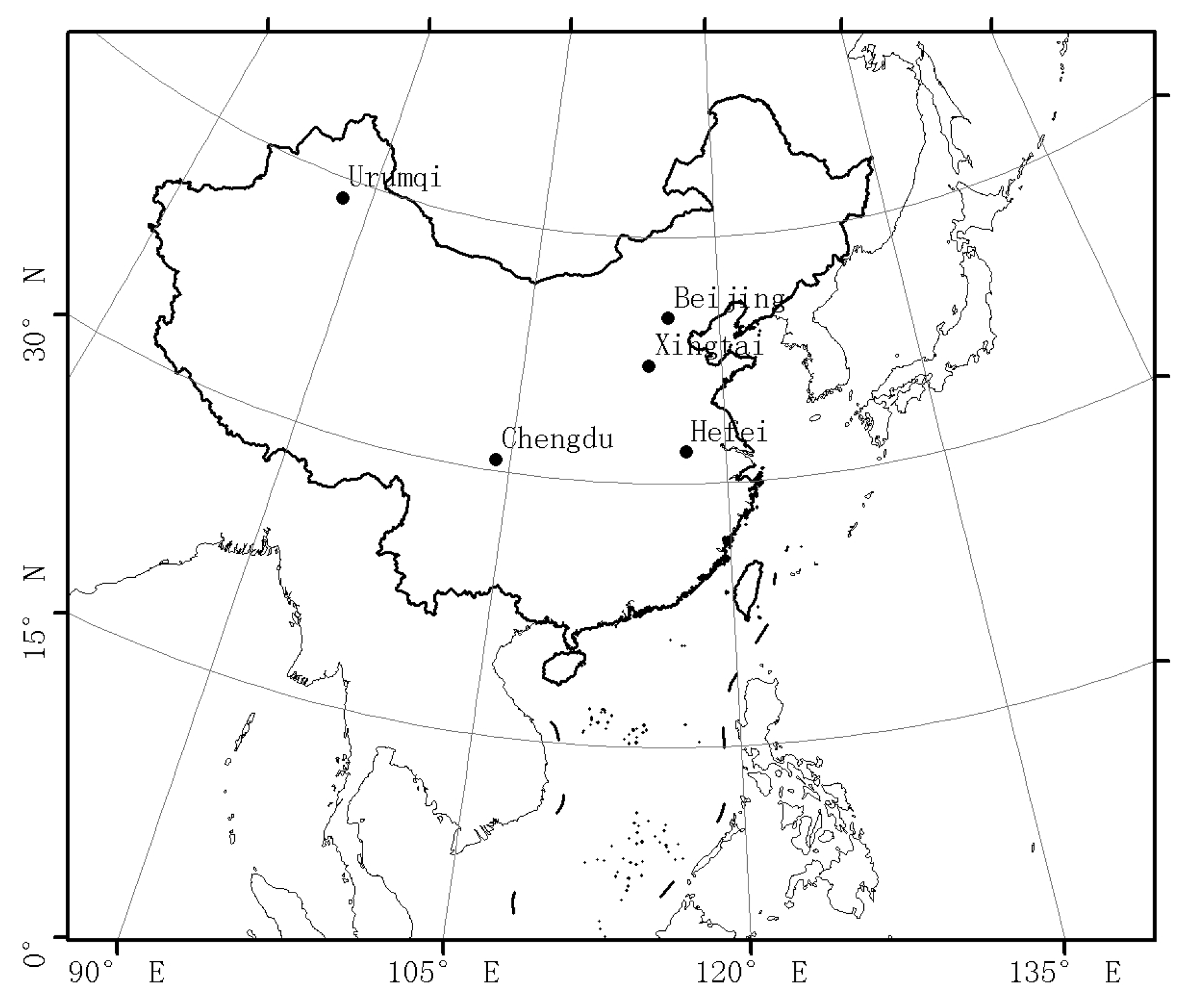
Figure 1. Model domain for RAMS-CMAQ used in this study is on a rotated polar stereographic map projection centered at (35°N, 116°E) with a 64 km grid cell.
Remotesensing 09 00519 g001
Figure 2. Distribution of the 100 ground-level NO2 concentrations CNEMC monitored stations.
Remotesensing 09 00519 g002
Figure 3. Scatter plots to verify accuracy of vertical distribution of tropospheric NO2 profiles over China from the RAMS-CMAQ model in January, April, July and October in 2014.
Remotesensing 09 00519 g003
Figure 4. The simulated NO2 vertical profiles over Beijing (a), Xingtai (b), Chengdu (c), Urumqi (d) and Hefei (e) in January, April, July and October in 2014.
Remotesensing 09 00519 g004
Figure 5. Monthly derived ground-level NO2 concentrations over China in January, April, July, and October in 2014.
Remotesensing 09 00519 g005
Figure 6. Line charts of the derived ground-level NO2 concentrations with in-situ measurements from ground network and the RAMS-CMAQ simulation over Beijing, Xingtai, Chengdu, Urumqi and Hefei cities in 2014.
Remotesensing 09 00519 g006
Figure 7. Scatter plots of the derived ground-level NO2 concentrations with in-situ measurements from ground network (a) and the RAMS-CMAQ simulation (b) over China in January and July 2014.
Remotesensing 09 00519 g007
Table 1. The information of the selected five cities.
City NameLatitudeLongitudeCity Condition
Beijing40.00°116.00°a megalopolis located in northeastern China that presents relatively high levels of air pollution
Xingtai37.05°114.48°one of the most air-polluted cities in China, and an important energy base in the North China area
Chengdu30.67°104.06°a large city located in southwestern China with relatively high air pollution compared to other southwestern cities
Urumqi43.77°87.68°a large city located in northwestern China but with lower levels of air pollution compared to other cities located in the east
Hefei31.86°117.27°a large city located in southeastern China with relatively low levels of air pollution compared to other cities located in the north

