
Optical Cloud Pixel Recovery via Machine Learning


Department of Civil, Environmental and Construction Engineering, University of Central Florida, Orlando, FL 32816, USA
*
Author to whom correspondence should be addressed.
Remote Sens. 2017, 9(6), 527; https://doi.org/10.3390/rs9060527
Submission received: 14 December 2016
/
Revised: 19 May 2017
/
Accepted: 21 May 2017
/
Published: 25 May 2017
Abstract
:Remote sensing derived Normalized Difference Vegetation Index (NDVI) is a widely used index to monitor vegetation and land use change. NDVI can be retrieved from publicly available data repositories of optical sensors such as Landsat, Moderate Resolution Imaging Spectro-radiometer (MODIS) and several commercial satellites. Studies that are heavily dependent on optical sensors are subject to data loss due to cloud coverage. Specifically, cloud contamination is a hindrance to long-term environmental assessment when using information from satellite imagery retrieved from visible and infrared spectral ranges. Landsat has an ongoing high-resolution NDVI record starting from 1984. Unfortunately, this long time series NDVI data suffers from the cloud contamination issue. Though both simple and complex computational methods for data interpolation have been applied to recover cloudy data, all the techniques have limitations. In this paper, a novel Optical Cloud Pixel Recovery (OCPR) method is proposed to repair cloudy pixels from the time-space-spectrum continuum using a Random Forest (RF) trained and tested with multi-parameter hydrologic data. The RF-based OCPR model is compared with a linear regression model to demonstrate the capability of OCPR. A case study in Apalachicola Bay is presented to evaluate the performance of OCPR to repair cloudy NDVI reflectance. The RF-based OCPR method achieves a root mean squared error of 0.016 between predicted and observed NDVI reflectance values. The linear regression model achieves a root mean squared error of 0.126. Our findings suggest that the RF-based OCPR method is effective to repair cloudy pixels and provides continuous and quantitatively reliable imagery for long-term environmental analysis.

1. Introduction
Normalized Difference Vegetation Index (NDVI) conveys valuable information relating to vegetation properties on the land surface [1,2]. NDVI is a vegetation index derived from optical remote sensors and represents the reflective and absorptive characteristics of vegetation in the red and near infrared (NIR) bands of the electromagnetic spectrum. For this reason, a chronological analysis of NDVI can indicate changes in vegetation conditions proportional to the absorption of photo-synthetically active radiation [3]. Such time series analyses of NDVI can detect the impact of natural events or anthropogenic disturbances on vegetation and can play an important role in natural resource management [4]. Furthermore, NDVI change detection can provide multi-dimensional information such as differences in urban land use/land cover changes [5], vegetation dynamics, surface elevation and floodplain dynamics [6].
The raw data for NDVI can be downloaded at no cost from several publicly available optical remote sensor repositories such as the Advanced Very High Resolution Radiometer (AVHRR), Moderate Resolution Imaging Spectro-radiometer (MODIS)-TERRA, MODIS-AQUA and Landsat satellites. Commercial satellites such as Satellite Pour l'Observation de la Terre (SPOT) also provide NDVI information. Among the publicly available sensors, Landsat has longest data record and is applicable for modeling terrestrial ecosystems on global, continental, and regional scales.
The main drawback of Landsat, as with any optical satellite sensor, is that the imagery can be obscured, shadowed, or saturated. The effects of clouds and cloud shadows, atmospheric variability, and bi-directional effects include the outright omission or skewing of readings in the image. These issues hamper the monitoring of terrestrial ecosystems and introduce undesirable noise [7,8]. This is especially significant in change detection analyses at climatic time scales. Errors due to the presence of clouds introduce uncertainties in satellite images during information retrieval, signal processing, data compression and distribution procedures causing anomalous results that are often difficult to correct [9,10].
Data reconstruction has recently gained popularity in Remote Sensing (RS). Spatial reconstruction has been described by removing cloud-contaminated portions in satellite images and cloning information from cloud-free patches [11]. Reconstruction of cloudy areas has also been proposed based on compressive sensing (CS) theory in underdetermined linear equation systems [12]. For example, a recently developed method uses two multi-temporal dictionary learning methods based on the expanded K-means clustering process and Bayesian algorithms [11]. Furthermore, at the acquisition layer, the commonly used Landsat NDVI data products are multi-day Maximum Value Composite (MVC) [13]; however, some noise remains in the final imagery. Data from Landsat, or optical satellites in general, are frequently discontinuous and faulty in warm coastal areas such as Florida’s gulf and west coasts due to heavy near shore evapotranspiration [14]. Therefore, it is crucial to mitigate or eliminate faulty information and recover missing information in a defensible and repeatable manner to enhance NDVI as a viable tool for long term change detection analyses.
To this end, an information recovery method, named Optical Cloud Pixel Recovery (OCPR), is proposed here to reconstruct the values of cloudy pixels through the established multi-parameter time-space-spectrum relationships of cloud-free pixels. The proposed OCPR method is able to predict NDVI using a random forest (RF) model trained and tested on a large high resolution spatio-temporal multi-parameter (temperature, precipitation, water level and months) data set and assess its performance in terms of information recovery from cloud coverage in remotely sensed Landsat MVC images. A comparison of the performance of RF with linear regression and mean only methods to predict NDVI is also included to justify the complexity of the RF model.
2. Past Research on Data Recovery
The importance of data recovery in numerous fields such as medical [15,16], neuro-computation [17], and climate science [18,19] has long been realized. Several approaches have been applied to recover the value of missing data. These methods were developed using statistical and numerical models to recover missing values from the originally available data. There were numerous relevant studies that have been conducted to recover either NDVI or other similar data by combination of time-space-spectrum memory. Based on the type of study, here we divide the literature review in three groups. First are studies on NDVI value recovery using empirical methods; second are studies on data recovery using machine learning methods; and third are studies on hydrologic parameters and their relationship with NDVI. While the first two sections of literature review explore existing data recovery methods, the third section provides insight into additional relevant variables that can be utilized to develop a novel model to recover Landsat NDVI values from beneath cloud cover. Typically, missing data may arise from instrumental error, time-lapse, and limited field visits. In the field of optical remote sensing, the missing data primarily originate from clouds. It is difficult to systematically reconstruct information under cloudy pixels at regional or larger scales with sufficient accuracy, especially, in warm coastal areas with frequent storms and broad cloud cover. In addition, due to the stochastic nature of clouds, it is difficult to build a consistent relationship to recover the value of pixels beneath the clouds. Therefore, inclusion of additional influential variables in long time-series data presents an opportunity to build a robust data recovery model with sufficient training data.
2.1. Data Recovery Using Empirical Methods
A number of methods for reducing noise and building high-quality NDVI time series data sets have been proposed, applied, and examined in the last two decades in accordance with data availability and research applications. However, research into the recovery of missing NDVI pixels due to cloud cover is limited. The most common and widely used NDVI cloud pixel recovery methods are threshold-based methods such as the best index slope extraction algorithm (BISE) [20]; Fourier-based fitting methods [21,22]; and asymmetric function fitting methods such as the asymmetric Gaussian function fitting approach [23] and the weighted least-squares linear regression approach [24]. Some simpler approaches were also practiced before the year 2000 such as substitution and interpolation. Substitution approaches were used to fill in cloudy pixels using information from adjacent cloud-free pixels in the same image. Otherwise information was retrieved for the corresponding pixels from previous time periods [25,26]. In addition to methods applied directly to NDVI, data recovery techniques for other types of similar data are also informative. Several studies have used similar techniques to estimate missing rainfall data including inverse distance weighting [18], expectation maximization algorithm [19], and regression [27].
Cloud removal is a topic being studied by many researchers in the field of RS. Shen et al. [28] provided an overview to the theories and principles of missing information reconstruction of RS data and described conventional and emergent algorithms under four main categories; (1) spatial-based; (2) spectral-based; (3) temporal-based; and (4) hybrid. They argued that while the spatial-based methods cannot reliably reconstruct data if information over large areas is missing, spectral-based methods are capable of performing well in similar situations based on the spectral correlations. Multi-temporal dictionary learning algorithms have been able to efficiently reduce clouds and accurately reconstruct contaminated surficial information underlying large-scale clouds and shadows [29]. A new patch matching multi-temporal group sparse representation (PM-MTGSR) method has also been proposed for the reconstruction of the optical remote sensing missing data [26]. They suggested that the method is suitable for thick cloud cover or cases of sensor failure. In the PM-MTGSR method, the required auxiliary images are normalized to reduce their difference from target image and both auxiliary and target images are reordered to two dimensions and separated into a sequence of partially overlapping patches. Li et al. [30] investigated the reconstruction of RS images in the framework of sparse representation and established that sparse representation methods perform better than representative methods for reconstructing RS images.
A major issue regarding cloud pixel recovery is the resolution mismatch between the input predictors and predicting target. The coarse resolution data normally have high temporal frequency thus temporal information can be important for information reconstruction, although temporal information is rare in the 30 m resolution data. The methods for reconstruction of 30 m resolution data can be divided into spatial based, temporal based and auxiliary sensor based depending on the information utilized.
2.2. Data Recovery Using Machine Learning Methods
Machine learning has been applied to recover numerous types of data in various fields of study and has been proven to produce reasonable relationships from small datasets while remaining relatively robust in the presence of noisy or missing input [31]. This is mainly the result of their capability to capture complex, nonlinear and dynamic relationships in function generalization and regression as well as classification of data. Specifically, evolutionary algorithms, including genetic programming, feed forward back propagation neural networks, support vector machines, and deep learning algorithms [12,31,32] are effective at recognizing subtle patterns and thus have been employed to characterize the complex relationships between the cloudy and cloud-free pixels in the historical time series over spatial and spectral domains [15]. However, clustered missing data such as seasonal storm clouds over multiyear time scales make the compilation of viable training and test data difficult. To combat this, ancillary predictor variables can aid in developing models to capture the variability of the data. Choosing and developing these ancillary variables for use in change detection analyses requires that they have compatible spatial and temporal scales. Therefore, most conventional methods have suffered from lower learning capacity which hampered their applicability in broader contexts.
Decision tree based methods such as Random Forests (RF) [33] are recognized for their ability to recover missing values as well as accommodate high dimensional data and complex relations among variables. For example, RF has been used to improve the prediction of missing values using laboratory generated medical data [16] and also to classify salt marsh vegetation [34]. In general, RF is a decision tree based method for classification and regression. It is an ensemble of multiple decision trees, or a set of hierarchically ordered conditions that produce individual predictions (i.e., class or regression value) which are then aggregated into a single prediction by majority vote (classification) or averaging (regression). The conditions are sequentially applied to a randomly selected subset of the data from a root (parent) node to a terminal (or child) node to make repeated predictions of the phenomenon represented by training data [33]. The child nodes can be thought of, metaphorically, as the leaf of a tree. The trees used in developing the RF algorithm are referred to as Classification and Regression Trees (CARTs). The prediction of missing data values is generally achieved through a model developed by the algorithm and a set of training data. The model contains a number of CARTs set by the model developer. Training and testing (and sometimes validation) datasets are extracted from the total data corpus to train the model and then test (and validate) the model’s prediction capabilities. The predictions for a RF regression model are trained by finding the mean of all the predictions of each CART that best minimize the error function. Each decision tree in a RF utilizes a randomly chosen subset of the training data, with replacement, so that each tree in the ensemble samples from the entire training dataset [35]. The prediction output of the RF is the average prediction from all regression trees in the forest or ensemble, or the classification receiving the highest number of “votes”. Recursive splitting and multiple classifications or regressions are carried out to run the analysis of the decision trees [36].
2.3. Hydrologic Parameters and Their Relationship with NDVI
Barbosa and Lakshmi Kumar [37] showed the links between NDVI and rainfall in north eastern Brazil. They explored vegetative drought in the region and found rainfall (or lack thereof) as the dominant causative factor in the event. Fu and Burgher [38] found that the maximum temperature primarily splits NDVI values, followed by previous rainfall and then inter-flood dry period and resulting groundwater levels and suggested that warmer months required more rain compared to cooler months to attain similar mean NDVI values in areas of high NDVI such as riparian zones, likely due to higher local evaporation. Inter-flood dry periods were also found to be important for maintenance of NDVI levels, especially when rainfall is limited. Another contributing factor in NDVI dynamics is the groundwater level. Shallower groundwater levels tend to enhance NDVI and thereby vegetation greenness primarily due to the wetter environment [38]. Wang et al. [39] examined spatial responses of NDVI to precipitation and temperature during a 9-year period (1989–1997). Among the considered climatic factors, precipitation and temperature strongly influenced both temporal and spatial patterns of NDVI. Hao et al. [40] explored the linkage of NDVI to temperature and precipitation in northern china. The NDVI response for grassland and forest to three climatic indices (i.e., yearly precipitation and highest and lowest temperature) was analyzed showing that the yearly precipitation and highest temperature were correlated with NDVI. To summarize the work done to date and illustrate the novelty of the proposed method, Table 1 shows previous missing data prediction methods along with their advantages and disadvantages.
A careful investigation of the literature showed that the most popular methods to recover missing data involve building relationships in time-space-spectrum domain between cloud and cloud-free pixels, which are useful as a historic memory of prevailing conditions. The addition of ancillary hydrologic data such as rainfall or water level, known to influence the vegetation characteristics, can enhance the predictive performance of models capable of synthesizing disparate data sources. The investigation regarding the complex methods and links between NDVI and other climatic parameters guides the selection of predictor variables and also methods. Powerful tools, machine learning for example, are needed to characterize these complex relationships accurately and efficiently. To that end, the current study developed an OCPR method based on the Random Forest algorithm and assessed its performance for NDVI recovery beneath cloud obscured or otherwise faulty pixels. The OCPR method is applied to remotely sensed Landsat MVC images and compared to a linear regression model. A comparison to a simple spatial mean method is also performed to justify the complexity of the RF model.
3. Methods and Material
The objective of this study is to recover NDVI values from beneath cloudy and faulty pixels within Landsat MVC imagery. The method is based on three assumptions: (1) NDVI data are a proxy for vegetation vigor, therefore a monthly NDVI time series will follow the annual cycle of growth and decline; (2) The “cfmask” product provided with Landsat MVC imagery accurately identifies clouds and cloud shadows [43]; (3) coastal NDVI dynamics are related to local hydrologic variables rainfall, temperature, and water (tide) level [18,19]. In line with these three assumptions, the OCPR method was developed. In the following sections, a brief description of the study area is provided, followed by the OCPR method development and assessment. Figure 1 presents a flowchart that summarizes the methodology.
3.1. Study Area
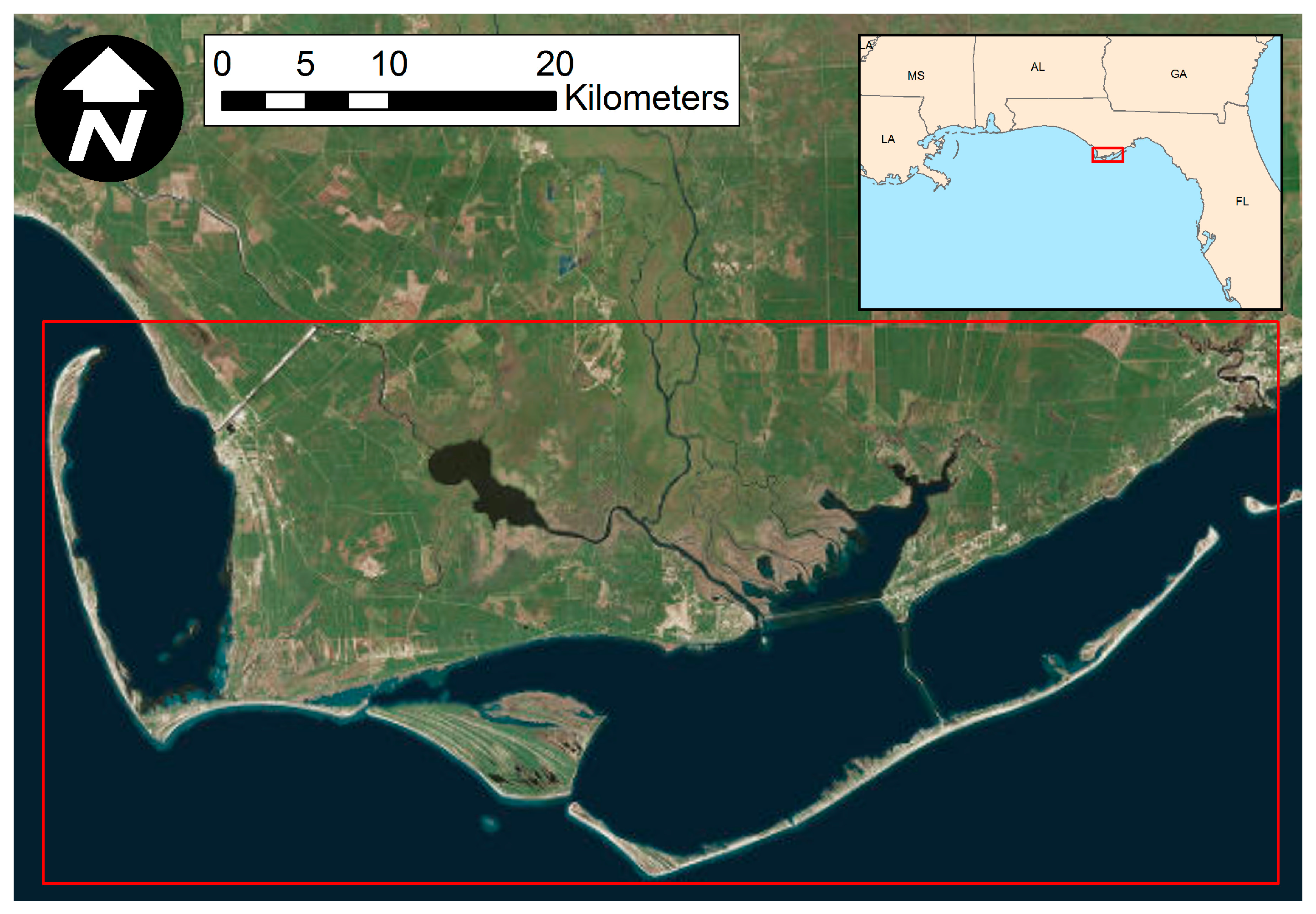
The study area occupies a section of Landsat TM scene L4-5 TM, Path 19/Row 39, located in Apalachicola Bay, Florida (see Figure 2). Apalachicola Bay is renowned for the largest oyster fishery in Florida [44] and is home to a rich variety of wetland plant, animal and microbial species. The lower Apalachicola river region as a whole is a nearly uninterrupted series of natural salt marshes, swamps, upland vegetation, and flood plains. Much of the basin vegetation has the appearance of a mature forest because of rapid regrowth. Although some municipalities (Apalachicola and Eastpoint) are situated near or within the riverine and tidal flood plains, they are not major urban centers. Therefore, there is very little urbanization in the basin. The study area includes parts of Gulf and Franklin counties. Wetland areas, including forested and non-forested wetlands, make up about 42% of the study area excluding open water and urban areas. The non-wetland and non-forested areas are mainly covered by agriculture, buildings and invasive vegetation.
3.2. Optical Cloud Pixel Recovery (OCPR)
The proposed method computes an NDVI value for cloudy or faulty pixels through an empirically trained RF model. The base dataset is composed of the relevant spatially distributed hydrologic time series data associated with the available body of Landsat MVC NDVI images. The predictor variables include mean monthly temperature, cumulative monthly precipitation, mean monthly water (tide) level, calendar month encoded as a sequential number from 1 to 12, northing and easting (coordinates in meters). The objective of the study is to train and test the model using historic data and validate its performance in terms of its ability to accurately recover hypothetical (i.e., synthetic, known NDVI) cloudy pixels manually inserted into the validation images.
Random Forest
The RF algorithm is initiated by dividing the target variable or parent node into binary parts, and each generation of child nodes are purer than their parent node. Throughout this procedure, the decision tree progresses through all candidate splits to determine the optimal split that maximizes the purity of the resulting tree. Residual sum of squares (RSS), shown in Equation (1) is used as the splitting criteria.
where, and refer to the left and right nodes, determined by the binary split.
While classic regression trees are typically “pruned” (reducing the number of leaves or child nodes) according to a specific condition, decision trees in RF grow to maximum purity, constrained in most computer implementations by a maximum depth parameter. Each tree may share similar or different conditions as set by the model developer. Each tree sees only part of the training data sets and thus captures only part of the information it contains. All of the trees look quite similar to each other and therefore the predictions from the trees can be highly correlated. The details of RF can be found in [45,46]. The RF algorithm uses the Gini impurity index [47] to calculate the information purity of child nodes compared to that of their parent node. From the parent node, the data splitting process in each internal node of a condition of the tree is repeated until a pre-specified stop condition is reached. Each of the child nodes has a simple regression model attached to it, which applies to that node only.
It has been observed in several studies that the RF algorithm offers characteristics that make it appealing for different applications. These include built-in feature selection capabilities, relatively high levels of accuracy in predictions, and a means for evaluating the influence of each feature on the algorithm [48]. The theoretical background of RF regression is discussed in detail in [33,49,50]. The essential attribute of RF is that it trains each tree individually, using a bootstrap sample of the data. This randomness helps to make the model more robust than a single decision tree and less likely to over fit to the training data. The ensemble of decision trees aggregates predictions of continuous variables by averaging the predictions from all trees. Random vectors are often generated in order to grow each tree in this ensemble of decision trees [33]. A popular example of this is bootstrap aggregation, commonly referred to as bagging, where a random subset is selected with replacement to train the individual trees with the results of the ensemble aggregated by averaging or voting [35,50].
The RF algorithm also provides an additional level of randomness to the bagging process. While nodes of standard decision trees are split by making use of the best possible split from the full list of predictor variables, RF uses a randomly selected subset of these variables; this drastically speeds up the tree growing process. However, the RF procedure is such that every node utilizes the best possible split from the randomly selected subset of predictors at the node to perform the splitting procedure. The best splitter might either be the best overall, or just a fairly good splitter, or may not be of any help at all. If the splitter is not very helpful, the outcome from the split is two nodes that are essentially the same. One of the major benefits of the RF algorithm is that it is very easy to implement because there are only two important control variables: predictor sub-setting control for splitting at the nodes and the number of trees in the forest. Once sufficient values for these two parameters are determined, the algorithm is not particularly sensitive to them [51]. Figure 3a shows a synopsis of an ensemble with three trees while Figure 3b shows detail of one tree from the ensemble.
Critical parameters used to constrain a RF model are number of trees in the forest and maximum depth of the trees. Numerous opinions have been put forth for selecting the optimal value for each of the parameters. Previous research indicates that sometimes, a larger number of trees in a forest only increase its computational cost without any significant gain in performance. It is also possible that there is a threshold beyond which there is no significant gain, unless a huge computational environment is available. As the number of trees grows, it does not always mean the performance of the forest is significantly better than forests with fewer trees [52].
3.3. Application of OCPR in Apalachicola Bay
The schematic flowchart of the OCPR methodology is represented in Figure 1. The OCPR method includes five crucial steps: (1) data acquisition and input preparation (target: NDVI and predictors: temperature, precipitation, water level, month); (2) cloud and faulty value identification from NDVI; (3) selection of input for training OCPR model; (4) training, testing and building prediction model ; and (5) validation.
3.3.1. Data Acquisition and Input Preparation
Target Variable: NDVI
Surface reflectance NDVI data were acquired from the USGS Earth Resources Observation and Science (EROS) Center Science Processing Architecture (ESPA) archive for the years 1984 through 2015. Since OCPR is based on the historical time series of NDVI, a sufficient body of data is required to characterize the relationship between NDVI and its predictor variables.
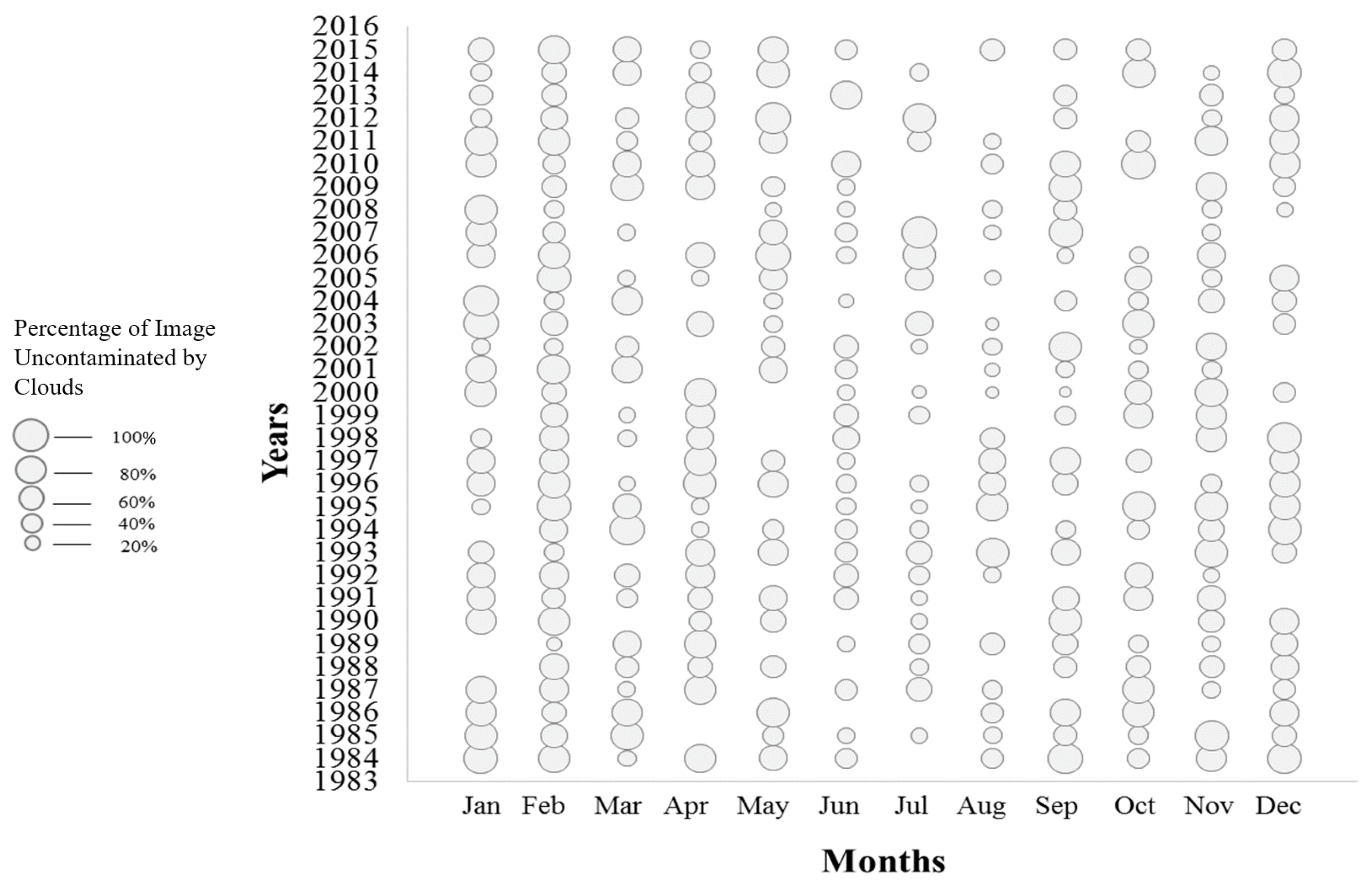
A threshold of 30% or less cloud cover (i.e., 70% of the pixels containing valid data) was used to screen the candidate Landsat MVC images over the above-referenced time period for inclusion, resulting in 252 usable images out of 384 (see Figure 4). Since NDVI is released as a 16-day composite, two images per month are often available. Considering that the month is a predictor variable in the feature vector, when two images were available for a given month the one with less cloud coverage was selected. Overall, 93% of the images were from Landsat-5 as it was the only data source from 1984 to 1998 and continued to acquire data until 2013. Landsat-7 data were avoided as it was contaminated by stripes as a result of the scan line corrector (SLC) in the Landsat Enhanced Thematic Mapper Plus (ETM+) sensor that failed permanently in 2003 [53]. The remainder of the data came from Landsat-8.
In performing the NDVI OCPR, data availability was considered at the pixel level, as per-pixel cloud cover and the swath side overlap between two adjacent paths were evaluated. Ancillary cloud mask, cloud shadow mask, adjacent cloud mask, snow mask, and water mask were available from the USGS Earth Explorer for the study area and were used for data quality assessment (QA). The QA layer, namely “cfmask”, identified water, cloud, cloud shadow, and snow [43] and was included in the ESPA NDVI product used in this study.
After NDVI image acquisition, all images were registered and clipped to the spatial extent of the project. Spatial registration, projection and resampling using WGS1984 UTM Zone 16N was implemented to ensure that each 30 m pixel location was consistent throughout the time series. These two processes (i.e., spatial registration and spatial clipping) were implemented using ArcGIS. NDVI was calculated using NIR and RED spectral bands of a sensor system as shown in Equation (2):
where NIR and RED are spectral reflectance measurements acquired in the near-infrared and visible red regions, respectively.
Predictor Variables: Rainfall, Temperature, Water Level and Month
The data for the predictor variables rainfall and temperature were collected for similar 30 m spatio-temporal domain from the PRISM climate group based at Oregon State University. The PRISM Climate Group collects climate observations from a large number of monitoring networks and builds spatial climate datasets to analyze short and long-term climate patterns. Time series data for precipitation and temperature were available at a spatial resolution of 4 km and the temporal coverage starts from 1981 to the present. This dataset was available online free of charge. These data were modeled using climatologically-aided interpolation (CAI), which uses the long-term average patterns as first-guess of the spatial pattern of climatic conditions for a given month or day. CAI is robust against wide variations in station data density, which is necessary when modeling over long time spans. The data used herein were available based on either monthly or daily interpolation. Monthly average values were estimated from daily values by averaging. These data used all station networks and data sources collected by the PRISM Climate group. After the precipitation and temperature data collection for the time domain was complete, they were registered, projected and clipped to match the the NDVI data. Spatial resolution for each precipitation (mm) and temperature (Kelvin) pixel was resampled from 4 km to 30 m. Downscaling to higher resolution reallocated the existing information to correspond to the NDVI data size and resolution. The processed NDVI, temperature (°C) and rainfall (mm) images are shown in Figure 5.
Next, water level data over the same temporal domain were collected. Water level data were available from the U.S. National Oceanographic and Atmospheric Administration National Ocean Service (NOAA-NOS) at coastal gauge stations across the United States. One gauge station was located in the study area (8728690 Apalachicola, FL). Monthly water level data were collected in meters relative to the NAVD88 orthometric datum. The tide gauge data were added to the predictor variable vector and used as a proxy for prevailing water levels. If a storm surge event was experienced, the value would be higher and according to our current hypothesis and previous work, would lower the NDVI of impacted areas, especially freshwater wetlands [54]. Examples of input data records used to train and test the algorithm are shown in Table 2.
3.3.2. Cloud and Faulty Value Detection from NDVI
In order to ensure that the labeled data were clean for training/testing of the RF and linear regression, pixels were classified as cloudy or cloud-free. The “cfmask” layers were processed to make a binary map that reclassifies all erroneous pixels as “0.0” and the valid pixels as “1.0”. A raster multiplication was done using the binary reclassified map and the NDVI images. This function removes the faulty values from the NDVI time series and replaces them with a void pixel. Since the data were collected from different sources, each dataset had their own label for anomalous data. For instance, NDVI time series gives “NaN” to a void pixel. After this preprocessing step, images were generated for each month of each year and used to calculate the percentage of clear pixels (POC) over the area of interest as shown below.
where is the total number of cloudy pixels and is the total number of pixels (i.e., both cloudy and cloud-free pixels) in the image j.
3.3.3. Selection of Input for Training OCPR Model
It is important to select reliable inputs for the construction/training of the OCPR model. The final prediction performance is highly dependent on the trained model. Candidate training pixels are comprised of valid (cloud-free) target data along with its corresponding (by month and position) predictor data. Here, NDVI are the target data and temperature, rainfall, water level, month, northing, and easting are the predictor data. In addition, NDVI, temperature, rainfall, northing, and easting are gridded raster products and are therefore spatially variable, while month and water level were represented by single values for each image.
3.3.4. Building the Prediction Model
The random forest algorithm used in the current study was implemented in Python. The scikit-learn (sklearn) [55] module was used to train and run the RF model and the GDAL [56] module was used to extract the spatial information associated with the target and predictor variables from geo-referenced images. 70% of the data corpus was randomly selected, without replacement, as the training data with the remaining 30% held out for testing. Figure 3a,b depict a schematic of splitting conditions. For the maximum purity of the RF model, the records containing missing predictors (NaNs) were removed. Overall, the construction of the data corpus from the associated imagery took approximately 5 min on average for each date (approximately 342 km2) on a non-specialized laptop computer.
3.3.5. Validation and Performance Metrics
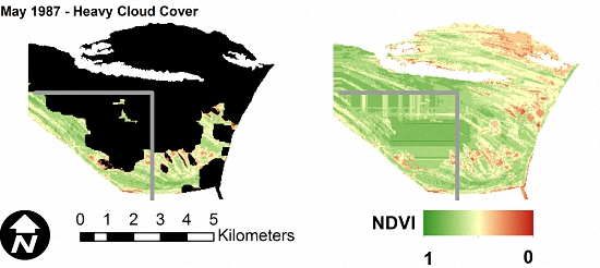
The prediction accuracy of the OCPR model was evaluated against a linear regression (LR) model. For quantitative validation of the model, hypothetical clouds were created where the underlying image has viable NDVI values. This provides labeled data for validation purposes. The images selected for the hypothetical cloud validation were deliberately excluded from the training and testing data, but were still located in the study area. A performance matrix was developed for the hypothetical cloud pixels using RF-based OCPR model and LR based model. In addition, a demonstration of the method on images with low, medium and heavy natural cloud cover is presented. With a section of the real cloud validation images located outside the training area, we visually demonstrated the impact of position as a prediction feature. The real cloud validation images visually demonstrated the application potential of the new algorithm.
Root-Mean-Square Error (RMSE)
The root-mean-square error is defined as:
where represents the difference between the predicted and observed NDVI at space–time points and m is the number of the time series of observations for each location.
Coefficient of Determination (R2)
The coefficient of determination (R2), an overall measure of performance, is defined as:
where Sj and indicate the standard deviations of reconstructed and observed NDVI values, respectively. R2 measures the linear association between prediction and observation. However, it only performs well when data are normally distributed and is sensitive to large values and outliers.
4. Results
4.1. Suitability and Sensitivity Analysis of RF Model
The best and most stable result was found using three hydrological predictors (precipitation, temperature and water level) along with position (northing and easting) and month in the RF model. Table 3 shows that success-rate of RF model according to number of trees and maximum depth of trees, performed as a sensitivity analysis on a small subset of the data. Ten trees with a maximum depth of 30 was the optimal combination in this case as shown by the minimum RMSE and maximum R2. If we increased the number of trees and maximum depth beyond those values, we did not gain much improvement and the computation time significantly increased. Nielson et al. [57] noted that in “big data” settings, it is undesirable to grow the individual tree components of a RF ensemble to their maximal depth. More recently, Kertész argues that there is an optimal tree size beyond which the RF tends to overfit after growing too big without additional gain in the accuracy [58]. Therefore, all the hydrologic predictor variables were kept in the RF-based OCPR model with the selected number and maximum depth of trees.
4.2. Prediction of Missing Values Using OCPR
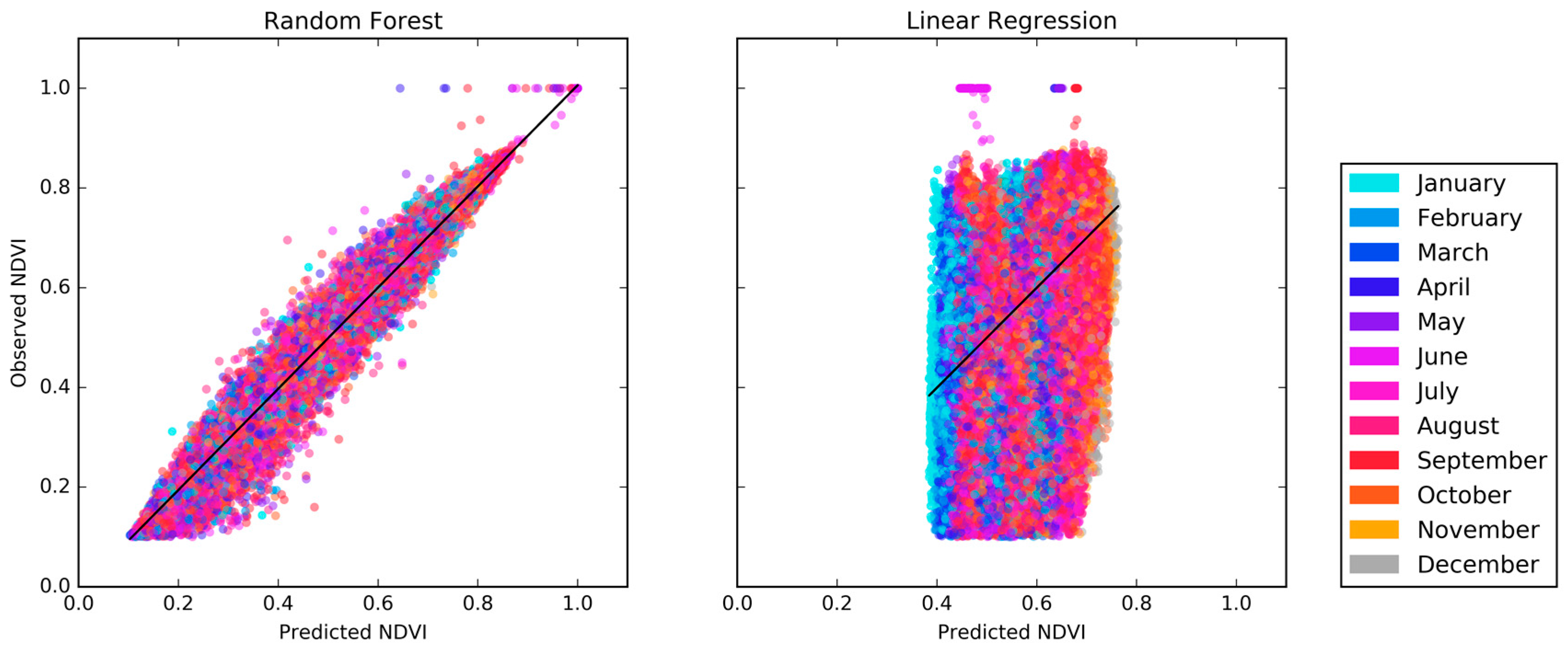
Figure 6 shows scatter plots of the predicted versus observed NDVI for the pixels in testing dataset for the OCPR model (Figure 6 (left)) and for the LR model (Figure 6 (right)). 30% of the total data corpus was selected, without replacement, to form the testing dataset. These results suggest that the OCPR model using hydrologic parameters outperforms the LR model in terms of prediction accuracy. For example, OCPR has an R2 value of 0.9880 and a clearly positive sloped linear trend while the LR model has a significantly weaker R2 value (0.2596) and much more scatter around its linear trend. The RMSE values shown in Table 4 also suggest that OCPR was able to reconstruct the cloudy pixels quite closely in terms of the absolute magnitude of NDVI. Based on this evidence, OCPR outperforms LR in terms of prediction accuracy. Additionally, OCPR model accuracy was compared with some other known empirical methods, such as S-G Golay, and Artificial Neural Network (ANN). For this, we randomly chose a few points from our NDVI data. Then we applied the OCPR method using ANN, RF, LR and S-G Golay. While the coefficient of determination (R2) were higher for both RF and ANN which were 0.4844 and 0.3244 respectively, the R2 were low for both LR and S-G Golay which were 0.0478 and 0.013, respectively.
The data shown in Figure 6 is also color coded by month to investigate the possibility of the model performing well as a whole while performing poorly in each individual month. The colors are well distributed throughout the scatter plot indicating that the model is performing equally well in each month in addition to the data aggregated over the entire time span.
The performance of OCPR was also validated by comparing the predicted and observed NDVI reflectance data for synthetic or hypothetical clouds manually applied to selected images that were held out of the training and test data. The result is shown in Figure 7. An area of naturally cloud-free pixels with heterogeneous nature was selected for demonstration, delineated as a black line square in Figure 7. These pixels were labeled as cloudy pixels. Then, the OCPR method was utilized to reconstruct the values of these pixels.
Image dates were selected so that the first date was before the study time period, the second date was near the middle and the final date was after. The three months were selected in three different times of year to capture seasonal variations, however the seasonal variations in this region are difficult to distinguish visually. The images are from October 1984, August 2002 and April 2015. These figures show that the OCPR model is capable of recovering missing NDVI values caused by cloud contamination with visually plausible results. The predictions did not produce any extremely low or high values of NDVI in the hypothetically clouded pixels.
5. Discussion
In this paper, a method for recovering NDVI values from beneath cloudy or otherwise faulty pixels is presented. This method, termed OCPR, was developed using a RF and is intended to address the issue of missing data in optical (visible and infrared) remote sensing images. This method takes advantage of the inherent capabilities and efficiencies of RF to characterize the relationship between NDVI and prevailing hydrologic parameters and spatial locations over the time-space spectrum. Inclusion of location (encoded as the northing and easting coordinates of the pixels) into the feature vector restricts model to reconstruct a value close to that of the neighboring pixels as well as a plausible value for that pixel in historical terms. In fact, as shown in Table 5, the position (Northing, Easting) of the pixel is the most important feature in the model. The other features contribute almost equally to the capture of the remaining variability, collectively accounting for 15.6% of the feature importance.
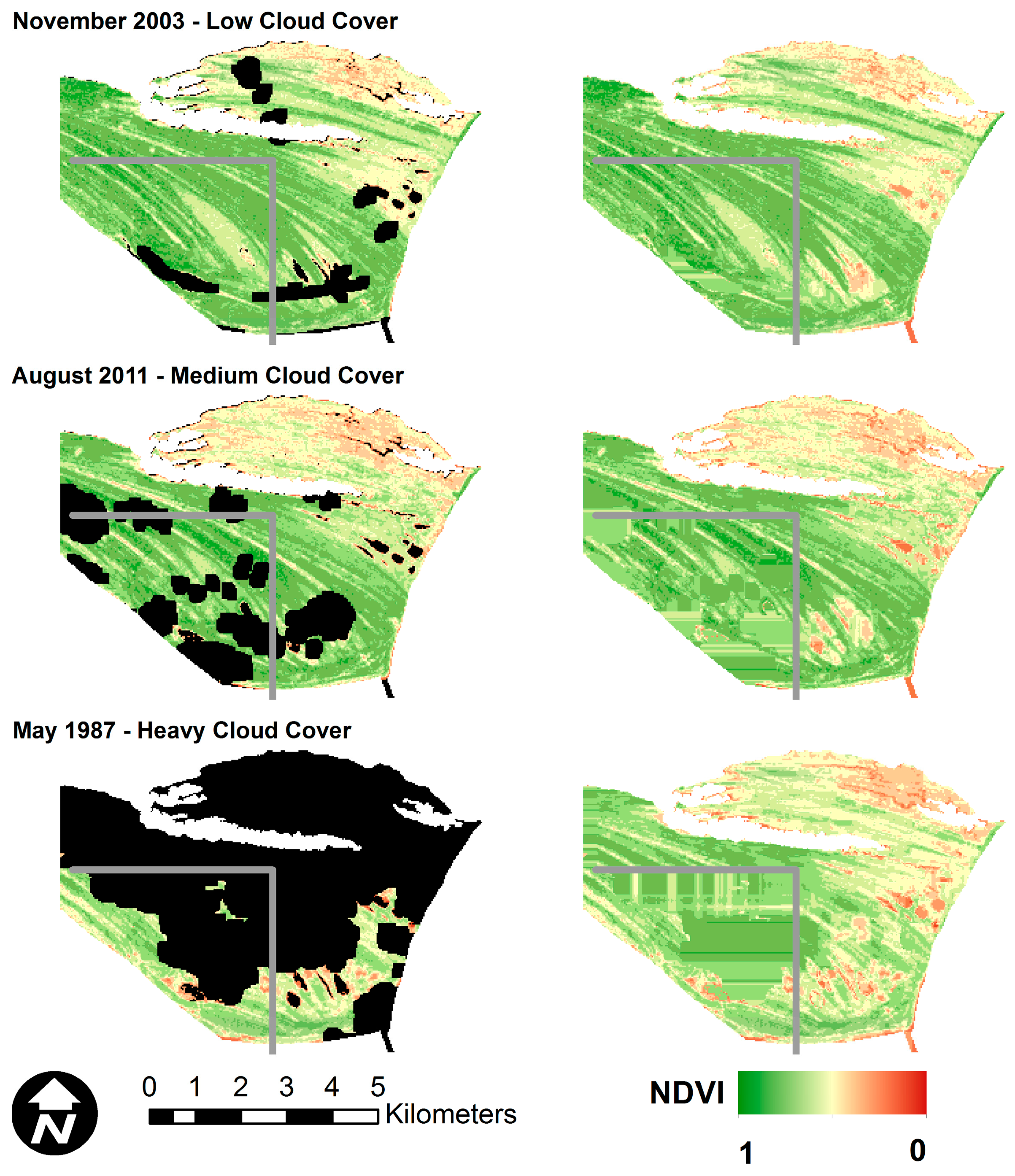
The performance of OCPR was further tested by applying the method to selected images with varying levels of natural cloud cover that were held out of the training and test data. In addition, a section of the image, delineated by gray lines in Figure 8, lies outside of the training data area. This was done to visually demonstrate the effect of spatial location on prediction accuracy.
As shown in Figure 8, OCPR is able to reconstruct the NDVI values beneath cloud pixels in a visually plausible manner. However, in all images, the section to the southwest of the gray lines appears smeared and horizontally oriented. As stated previously, this section of the image was not in the area used to train the random forest model at the core of OCPR. Therefore, the dominant importance of spatial location is evident. In addition, areas to the immediate north and west of the gray lines also show some visible distortion and unnatural uniformity. This indicates the presence of edge or boundary effects inherent in OCPR. Both of these issues point the user towards ensuring that the training data not only completely covers the desired area for OCPR application, but that the outer boundary of the training area lies well outside the area of interest.
The dominance of spatial position is an expected result due to the establishment of vegetative communities that persist over time. The hydrologic features serve to explain the relatively small changes in vegetation health (measured by NDVI) due to climatic factors. Two examples of this would be an increase in vegetation health due to above-average rainfall during the month, or perhaps a slight decrease in vigor due to a storm tide event that caused a higher average water level during the month (i.e., an increase in salinity causes vegetative stress for certain species). Future work will focus on testing the relative accuracy of a position only model, as well as testing the approach in different settings (upland vegetative communities, for example) and using different sensors.
Lastly, in terms of model training time, LR is significantly faster than RF. However, RF shows much better prediction accuracy than LR in this real world application based on the patches or spatial patterns of NDVI reflectance values. Also, the scale of the analysis presented herein correspond to a two county area in the United States. Regional or even global applications of OCPR will benefit from detailed scaling analysis and concern for efficient large scale computing efforts, including further code optimization and parallelization.
6. Conclusions
This study presents a technique for recovering data from beneath cloud contaminated pixels in optical remote sensing imagery. Specifically, the normalized difference vegetation index (NDVI) derived from Landsat imagery was recovered using a random forest based method named Optical Cloud Pixel Recovery (OCPR). Using spatial location (northing and easting), month (to capture seasonality), and hydrologic information known to influence coastal vegetation growth and vigor (rainfall, temperature and tide level) as predictor variables, OCPR was shown to be capable of reconstructing missing information in cloud contaminated regions with visually plausible and quantitatively accurate results, even under severe cloud cover situations. Spatial location (northing and easting) were the most important features in the model, with the remaining features collectively making up 15.6% of the feature importance. Over the test data set, OCPR recovered NDVI values with an RMSE of 0.016 (NDVI values range from 0 to 1). Also, the R2 for the observed versus predicted NDVI values was 0.988 (~1) indicating good reconstruction close to the original data.
The RF has many advantages in fast and accurate learning capability when characterizing complex time-space-spectrum relationships in real world studies. The proposed random forest based OCPR method is capable of recovering missing information with high efficacy and we predict that it can eventually be scaled for operational use.
It should be noted that the OCPR method was limited by the availability of the historical time series to characterize the complex time–spatial–spectral relationships between the cloudy and cloud-free pixels over the multiple parameters in a specific region. Also, the temperature, precipitation and water level predictor variables are currently not available at the spatial resolution of NDVI. This is most evident in the water level data as these are recorded in very limited locations such as NOAA-NOS tide gages. As with any machine learning model, including OCPR, its performance is heavily dependent on its training data. Improvements can be achieved by further optimizing the training algorithms and architectures of the random forest with the new ideas for treating missing values in the predictor variable data sets. Focusing on screening and selecting suitable inputs for the OCPR models is critical to the prediction accuracy. Also, the authors strongly recommend that the outer boundary of area selected for training lie well outside the area of interest in order to avoid edge or boundary effects, considering the importance of spatial location on the predicted values. In spite of these limitations, the idea of spatial information recovery via machine learning provides a promising and efficient approach to mitigate and eliminate cloud contaminations with sufficient accuracy over the long term remote sensing analyses.
Acknowledgments
This research is partially funded under Award No. NA10NOS4780146 from the National Oceanic and Atmospheric Administration (NOAA) Center for Sponsored Coastal Ocean Research (CSCOR) as well as by the U.S. Department of Homeland Security under Grant Award Number 2015-ST-061-ND0001-01. We thank the editor and three anonymous reviewers whose suggestions and constructive comments helped to improve the focus and presentation of our work. The views and conclusions contained in this document are those of the authors and should not be interpreted as necessarily representing the official policies, either expressed or implied of the U.S. Department of Homeland Security and the National Oceanic and Atmospheric Administration (NOAA) Center for Sponsored Coastal Ocean Research (CSCOR). The data presented in this paper can be requested from the authors.
Author Contributions
S.T. collected the data, developed and integrated the code, and wrote the paper under the supervision of S.C.M. and A.S. S.C.M. planned and designed the work, created Figure 5, Figure 6, Figure 7 and Figure 8, and developed and executed the code. A.S. guided the analysis and reviewed the paper. M.H. assisted in coding and reviewing the paper.
Conflicts of Interest
The authors declare no conflicts of interest.
References
- Justice, C.O.; Townshend, J.R.G.; Holben, B.N.; Tucker, C.J. Analysis of the phenology of global vegetation using meteorological satellite data. Int. J. Remote Sens. 1985, 6, 1271–1318. [Google Scholar] [CrossRef]
- Myneni, R.B.; Keeling, C.D.; Tucker, C.J.; Asrar, G.; Nemani, R.R. Increased plant growth in the northern high latitudes from 1981 to 1991. Nature 1997, 386, 698–702. [Google Scholar] [CrossRef]
- Sellers, P.J. Canopy reflectance, photosynthesis and transpiration. Int. J. Remote Sens. 1985, 6, 1335–1372. [Google Scholar] [CrossRef]
- Jovanović, M.M.; Milanović, M.M. Normalized Difference Vegetation Index (NDVI as the basis for local forest management. Example of the municipality of Topola, Serbia. Pol. J. Environ. Stud. 2015, 24, 529–535. [Google Scholar]
- Chen, J.; Jönsson, P.; Tamura, M.; Gu, Z.; Matsushita, B.; Eklundh, L. A simple method for reconstructing a high-quality NDVI time-series data set based on the Savitzky-Golay filter. Remote Sens. Environ. 2004, 91, 332–344. [Google Scholar] [CrossRef]
- Marchetti, Z.Y.; Minotti, P.G.; Ramonell, C.G.; Schivo, F.; Kandus, P. NDVI patterns as indicator of morphodynamic activity in the middle Parana River floodplain. Geomorphology 2016, 253, 146–158. [Google Scholar] [CrossRef]
- Cihlar, J.; Ly, H.; Li, Z.; Chen, J.; Pokrant, H.; Huang, F. Multitemporal, multichannel AVHRR data sets for land biosphere studies—Artifacts and corrections. Remote Sens. Environ. 1997, 60, 35–57. [Google Scholar] [CrossRef]
- Gutman, G.G. Vegetation indices from AVHRR: An update and future prospects. Remote Sens. Environ. 1991, 35, 121–136. [Google Scholar] [CrossRef]
- Eckardt, R.; Berger, C.; Thiel, C.; Schmullius, C. Removal of optically thick clouds from multi-spectral satellite images using multi-frequency SAR data. Remote Sens. 2013, 5, 2973–3006. [Google Scholar] [CrossRef]
- Melgani, F. Contextual reconstruction of cloud-contaminated multitemporal multispectral images. IEEE Trans. Geosci. Remote Sens. 2006, 44, 442–455. [Google Scholar] [CrossRef]
- Lin, C.H.; Tsai, P.H.; Lai, K.H.; Chen, J.Y. Cloud removal from multitemporal satellite images using information cloning. IEEE Trans. Geosci. Remote Sens. 2013, 51, 232–241. [Google Scholar] [CrossRef]
- Lorenzi, L.; Melgani, F.; Mercier, G. Missing-area reconstruction in multispectral images under a compressive sensing perspective. IEEE Trans. Geosci. Remote Sens. 2013, 51, 3998–4008. [Google Scholar] [CrossRef]
- Holben, B.N. Characteristics of maximum-value composite images from temporal AVHRR data. Int. J. Remote Sens. 1986, 7, 1417–1434. [Google Scholar] [CrossRef]
- Gutman, G.; Janetos, A.C.; Justice, C.O.; Moran, E.F.; Mustard, J.F.; Rindfuss, R.R.; Skole, D.; Turner, B.L., II; Cochrane, M.A. Land Change Science: Observing, Monitoring, and Understanding Trajectories of Change on the Earth’s Surface. Remote Sens. Digit. Image Process. 2004, 6, 482. [Google Scholar]
- Jerez, J.M.; Molina, I.; García-Laencina, P.J.; Alba, E.; Ribelles, N.; Martín, M.; Franco, L. Missing data imputation using statistical and machine learning methods in a real breast cancer problem. Artif. Intell. Med. 2010, 50, 105–115. [Google Scholar] [CrossRef] [PubMed]
- Hapfelmeier, A.; Hothorn, T.; Riediger, C.; Ulm, K. Estimation of a Predictor’s Importance by Random Forests When There Is Missing Data: RISK Prediction in Liver Surgery using Laboratory Data. Int. J. Biostat. 2014, 10, 165–183. [Google Scholar] [CrossRef] [PubMed]
- Sovilj, D.; Eirola, E.; Miche, Y.; Björk, K.-M.; Nian, R.; Akusok, A.; Lendasse, A. Extreme learning machine for missing data using multiple imputations. Neurocomputing 2015, 174, 220–231. [Google Scholar] [CrossRef]
- Simanton, J.R.; Osborn, H.B. Reciprocal-Distance Estimate of Point Rainfall. J. Hydraul. Div. 1980, 106, 1242–1246. [Google Scholar]
- Makhuvha, T.; Pegram, G.; Sparks, R.; Zucchini, W. Patching rainfall data using regression methods. 1 Best subset selection, EM and pseudo-EM methods: Theory. J. Hydrol. 1997, 198, 289–307. [Google Scholar] [CrossRef]
- Viovy, N.; Arino, O.; Belward, A.S. The Best Index Slope Extraction (BISE): A method for reducing noise in NDVI time-series. Int. J. Remote Sens. 1992, 13, 1585–1590. [Google Scholar] [CrossRef]
- Cihlar, J. Identification of contaminated pixels in AVHRR composite images for studies of land biosphere. Remote Sens. Environ. 1996, 56, 149–163. [Google Scholar] [CrossRef]
- Roerink, G.J.; Menenti, M.; Verhoef, W. Reconstructing cloudfree NDVI composites using Fourier analysis of time series. Int. J. Remote Sens. 2000, 21, 1911–1917. [Google Scholar] [CrossRef]
- Jonsson Lars Eklundh, P. Seasonality extraction by function-fitting to time-series of satellite sensor data. IEEE Trans. Geosci. Remote Sens. 2002, 40, 1824–1832. [Google Scholar] [CrossRef]
- Swets, D.L.; Reed, B.C.; Rowland, J.D.; Marko, S.E. A weighted least-squares approach to temporal smoothing of NDVI. In Proceedings of the ASPRS Annual Conference, from Image to Information, Portland, OR, USA, 17–21 May 1999; American Society for Photogrammetry and Remote: Portland, OR, USA, 1999. [Google Scholar]
- Long, D.G.; Remund, Q.P.; Daum, D.L. A cloud-removal algorithm for SSM/I data. IEEE Trans. Geosci. Remote Sens. 1999, 37, 54–62. [Google Scholar] [CrossRef]
- Lin, C.H.; Lai, K.H.; Chen, Z.B.; Chen, J.Y. Patch-based information reconstruction of cloud-contaminated multitemporal images. IEEE Trans. Geosci. Remote Sens. 2014, 52, 163–174. [Google Scholar] [CrossRef]
- Lynch, S.D. Development of a RASTER Database of Annual, Monthly and Daily Rainfall for Southern Africa; WRC Report No. 1156/1/04; Water Research Commission: Pretoria, South Africa, 2003; 78 p. [Google Scholar]
- Shen, H.; Li, X.; Cheng, Q.; Zeng, C.; Yang, G.; Li, H.; Zhang, L. Missing Information Reconstruction of Remote Sensing Data: A Technical Review. IEEE Geosci. Remote Sens. Mag. 2015, 3, 61–85. [Google Scholar] [CrossRef]
- Li, X.; Shen, H.; Zhang, L.; Zhang, H.; Yuan, Q.; Yang, G. Recovering quantitative remote sensing products contaminated by thick clouds and shadows using multitemporal dictionary learning. IEEE Trans. Geosci. Remote Sens. 2014, 52, 7086–7098. [Google Scholar]
- Li, X.; Shen, H.; Zhang, L.; Li, H. Sparse-based reconstruction of missing information in remote sensing images from spectral/temporal complementary information. ISPRS J. Photogramm. Remote Sens. 2015, 106, 1–15. [Google Scholar] [CrossRef]
- Ilunga, M.; Stephenson, D. Infilling streamflow data using feed-forward back-propagation (BP) artificial neural networks: Application of standard BP and pseudo Mac Laurin power series BP techniques. Water SA 2005, 31, 171–176. [Google Scholar] [CrossRef]
- Han, X.; Chen, X.; Feng, L. Four decades of winter wetland changes in Poyang Lake based on Landsat observations between 1973 and 2013. Remote Sens. Environ. 2015, 156, 426–437. [Google Scholar] [CrossRef]
- Breiman, L. Random forests. Mach. Learn. 2001, 45, 5–32. [Google Scholar] [CrossRef]
- Van Beijma, S.; Comber, A.; Lamb, A. Random forest classification of salt marsh vegetation habitats using quad-polarimetric airborne SAR, elevation and optical RS data. Remote Sens. Environ. 2014, 149, 118–129. [Google Scholar] [CrossRef]
- Breiman, L. Bagging Predictors. Mach. Learn. 1996, 24, 123–140. [Google Scholar] [CrossRef]
- Rodriguez-Galiano, V.F.; Chica-Olmo, M.; Chica-Rivas, M. Predictive modelling of gold potential with the integration of multisource information based on random forest: A case study on the Rodalquilar area, Southern Spain. Int. J. Geogr. Inf. Sci. 2014, 28, 1336–1354. [Google Scholar] [CrossRef]
- Barbosa, H.A.; Lakshmi Kumar, T.V. Influence of rainfall variability on the vegetation dynamics over Northeastern Brazil. J. Arid Environ. 2016, 124, 377–387. [Google Scholar] [CrossRef]
- Fu, B.; Burgher, I. Riparian vegetation NDVI dynamics and its relationship with climate, surface water and groundwater. J. Arid Environ. 2015, 113, 59–68. [Google Scholar] [CrossRef]
- Wang, J.; Price, K.P.; Rich, P.M. Spatial patterns of NDVI in response to precipitation and temperature in the central Great Plains. Int. J. Remote Sens. 2001, 22, 3827–3844. [Google Scholar] [CrossRef]
- Hao, F.; Zhang, X.; Ouyang, W.; Skidmore, A.K.; Toxopeus, A.G. Vegetation NDVI linked to temperature and precipitation in the upper catchments of Yellow River. Environ. Model. Assess. 2012, 17, 389–398. [Google Scholar] [CrossRef]
- Zhu, W.; Pan, Y.; He, H.; Wang, L.; Mou, M.; Liu, J. A changing-weight filter method for reconstructing a high-quality NDVI time series to preserve the integrity of vegetation phenology. IEEE Trans. Geosci. Remote Sens. 2012, 50, 1085–1094. [Google Scholar] [CrossRef]
- Tu, J.V. Advantages and disadvantages of using artificial neural networks versus logistic regression for predicting medical outcomes. J. Clin. Epidemiol. 1996, 49, 1225–1231. [Google Scholar] [CrossRef]
- Zhu, Z.; Woodcock, C.E. Object-based cloud and cloud shadow detection in Landsat imagery. Remote Sens. Environ. 2012, 118, 83–94. [Google Scholar] [CrossRef]
- Huang, W.; Hagen, S.; Bacopoulos, P.; Wang, D. Hydrodynamic modeling and analysis of sea-level rise impacts on salinity for oyster growth in Apalachicola Bay, Florida. Estuar. Coast. Shelf Sci. 2015, 156, 7–18. [Google Scholar] [CrossRef]
- James, G.; Witten, D.; Hastie, T.; Tibshirani, R. An Introduction to Statistical Learning: With Applications in R; Springer: Berlin, Germany, 2013; Volume XIV, ISBN 1461471370 9781461471370. [Google Scholar]
- Kuhn, M.; Johnson, K. Applied Predictive Modeling; Springer: New York, NY, USA, 2013; Volume 26. [Google Scholar]
- Breiman, L.; Friedman, J.H.; Olshen, R.A.; Stone, C.J. Classification and Regression Trees; Taylor & Francis: Park Drive, UK, 1984; Volume 19, ISBN 0412048418, 9780412048418. [Google Scholar]
- Palmer, D.S.; O’Boyle, N.M.; Glen, R.C.; Mitchell, J.B.O. Random forest models to predict aqueous solubility. J. Chem. Inf. Model. 2007, 47, 150–158. [Google Scholar] [CrossRef] [PubMed]
- Svetnik, V.; Liaw, A.; Tong, C.; Wang, T. Application of Breiman’s random forest to modeling structure-activity relationships of pharmaceutical molecules. In Proceedings of the International Workshop on Multiple Classifier Systems, Cagliari, Italy, 9–11 June 2004; pp. 334–343. [Google Scholar]
- Biau, G.; Devroye, L.; Lugosi, G. Consistency of random forests and other averaging classifiers. J. Mach. Learn. Res. 2008, 9, 2015–2033. [Google Scholar]
- Liaw, A.; Wiener, M. Classification and Regression by randomForest. R News 2002, 2, 18–22. [Google Scholar]
- Oshiro, T.M.; Perez, P.S.; Baranauskas, J.A. How many trees in a random forest? In Lecture Notes in Computer Science (Including Subseries Lecture Notes in Artificial Intelligence and Lecture Notes in Bioinformatics); Springer: Berlin/Heidelberg, Germany, 2012; Volume 7376, pp. 154–168. [Google Scholar]
- Goward, S.; Arvldson, T.; Williams, D.; Faundeen, J.; Irons, J.; Franks, S. Historical record of landsat global coverage: Mission operations, NSLRSDA, and international cooperator stations. Photogramm. Eng. Remote Sens. 2006, 72, 1155–1169. [Google Scholar] [CrossRef]
- Tahsin, S.; Medeiros, C.S.; Singh, A. Resilience of coastal wetlands to extreme hydrologic events in Apalachicola Bay. Geophys. Res. Lett. 2016, 43, 7529–7537. [Google Scholar] [CrossRef]
- Pedregosa, F.; Varoquaux, G. Scikit-learn: Machine learning in Python. J. Mach. Learn. Res. 2011, 12, 2825–2830. [Google Scholar]
- Warmerdam, F. GDAL—Geospatial Data Abstraction Library. 2012. Available online: http://gdal.org/1.11/ (accessed on 26 March 2016).
- Nielson, J.L.; Guandique, C.F.; Liu, A.W.; Burke, D.A.; Lash, A.T.; Moseanko, R.; Hawbecker, S.; Strand, S.C.; Zdunowski, S.; Irvine, K.-A.; et al. Development of a Database for Translational Spinal Cord Injury Research. J. Neurotrauma 2014, 31, 1789–1799. [Google Scholar] [CrossRef] [PubMed]
- Kertesz, C. Rigidity-Based Surface Recognition for a Domestic Legged Robot. IEEE Robot. Autom. Lett. 2016, 1, 309–315. [Google Scholar] [CrossRef]
Figure 1.
Schematic flowchart of the proposed OCPR method.
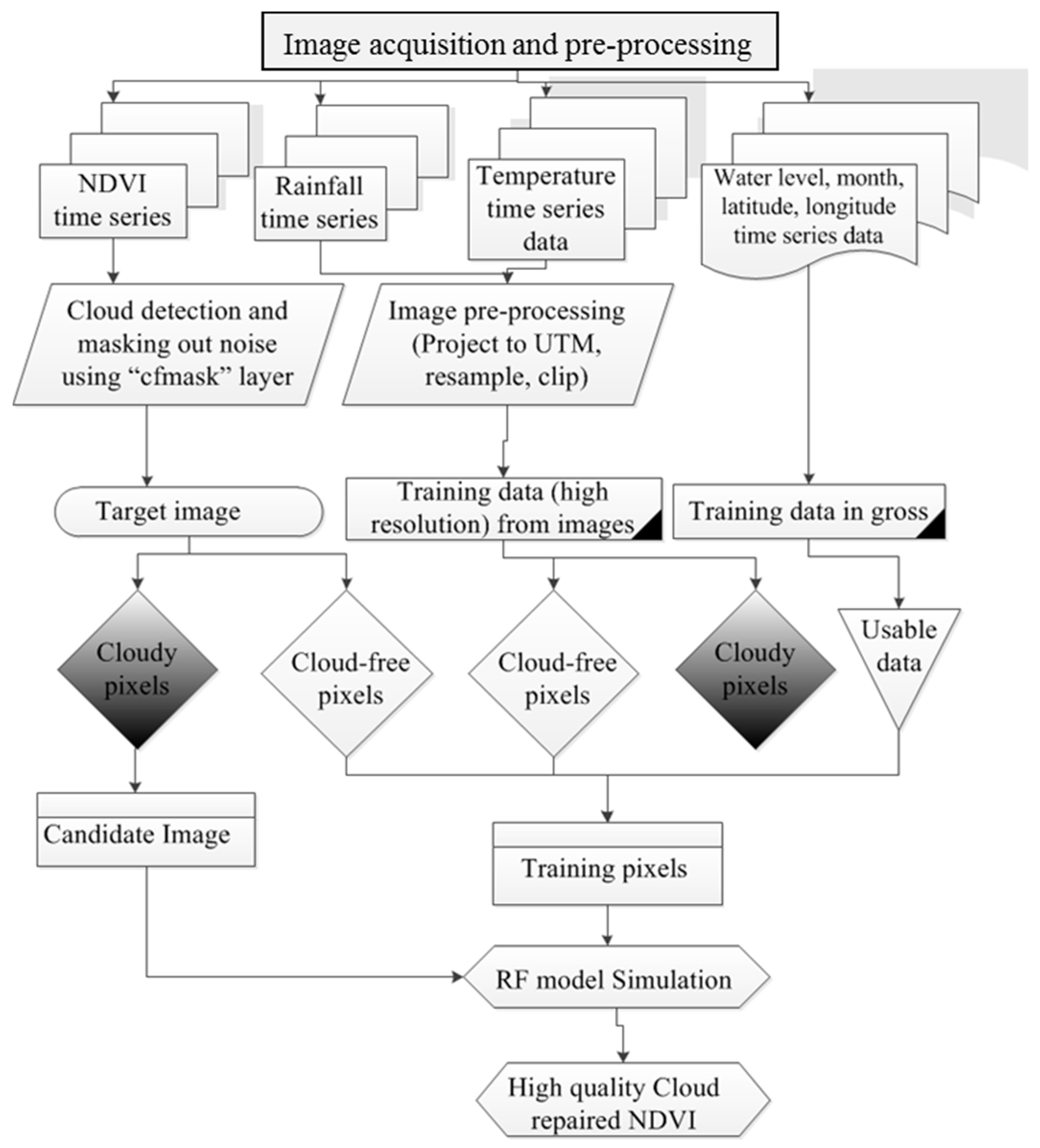
Figure 2.
Study Area in Apalachicola, Florida.

Figure 3.
Typical random forest regression tree structure (a) and example of an individual tree (b). M = month; R = rainfall, MT = maximum temperature; WL = water level; X1–X16 = splitting values.
Figure 3.
Typical random forest regression tree structure (a) and example of an individual tree (b). M = month; R = rainfall, MT = maximum temperature; WL = water level; X1–X16 = splitting values.
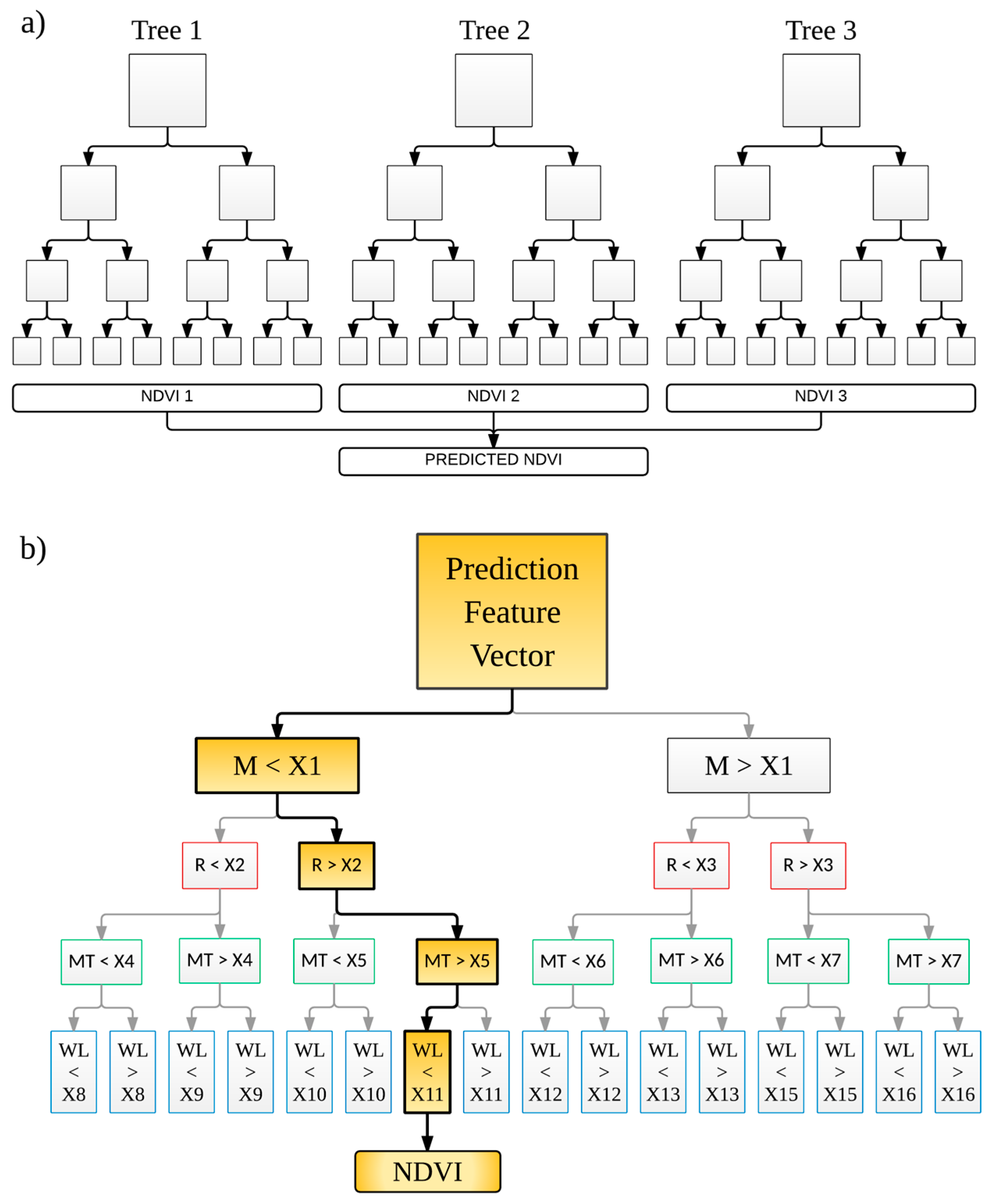
Figure 4.
Availability and usability of 16-day composite NDVI images over the study time period (1984–2015), bubble size indicates the % of available data in corresponding NDVI images.
Figure 4.
Availability and usability of 16-day composite NDVI images over the study time period (1984–2015), bubble size indicates the % of available data in corresponding NDVI images.

Figure 5.
Sample NDVI, rainfall, and temperature raster data.
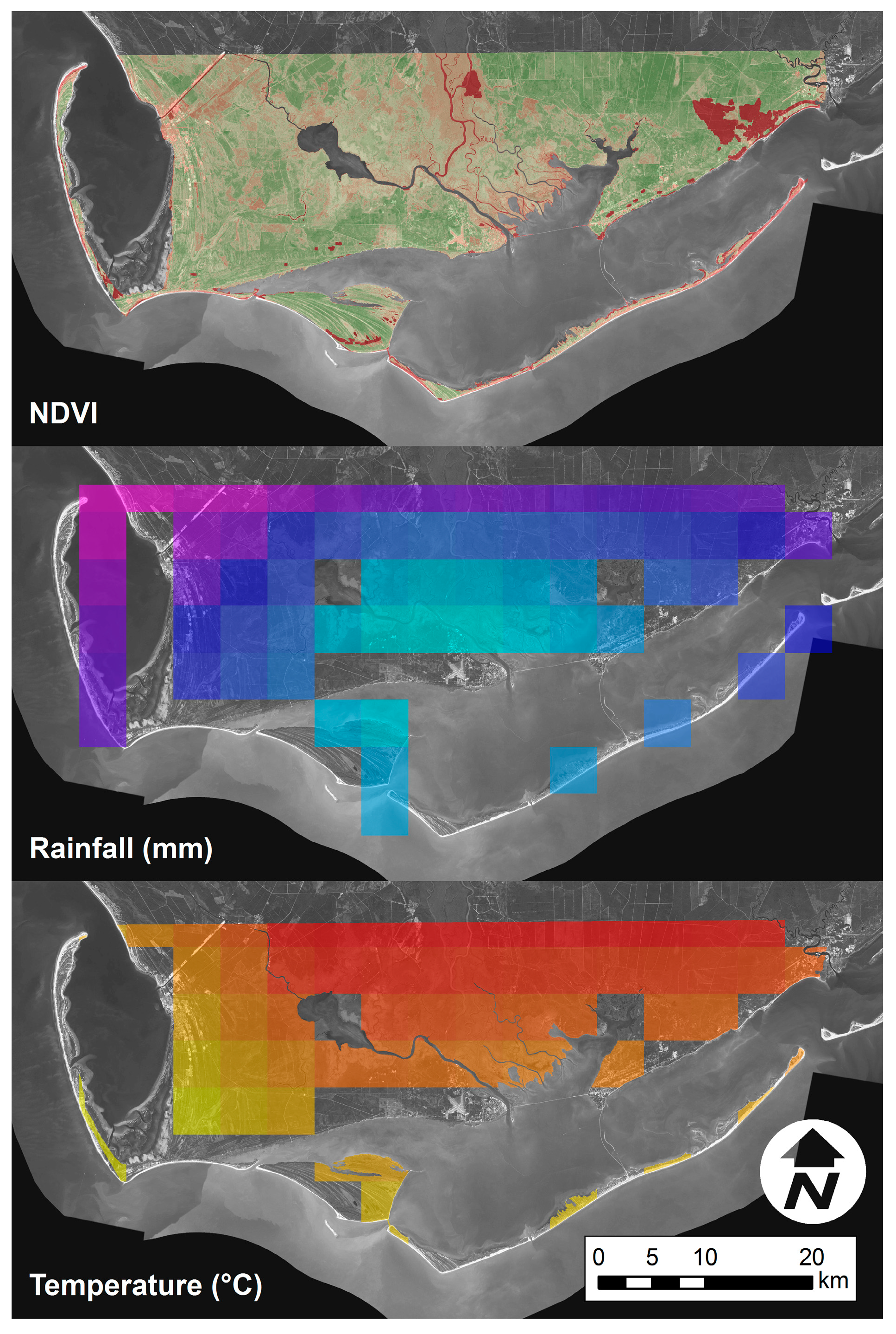
Figure 6.
Scatter plots of the observed and predicted NDVI from the testing dataset using (left) OCPR and (right) Linear Regression.
Figure 6.
Scatter plots of the observed and predicted NDVI from the testing dataset using (left) OCPR and (right) Linear Regression.

Figure 7.
Application of OCPR model to reconstruct NDVI under hypothetical clouds from images associated with October 1984, August 2002 and April 2015. The left column represents the original images and the right column represents the information recovered by OCPR. All images are visually symbolized using the same color scale.
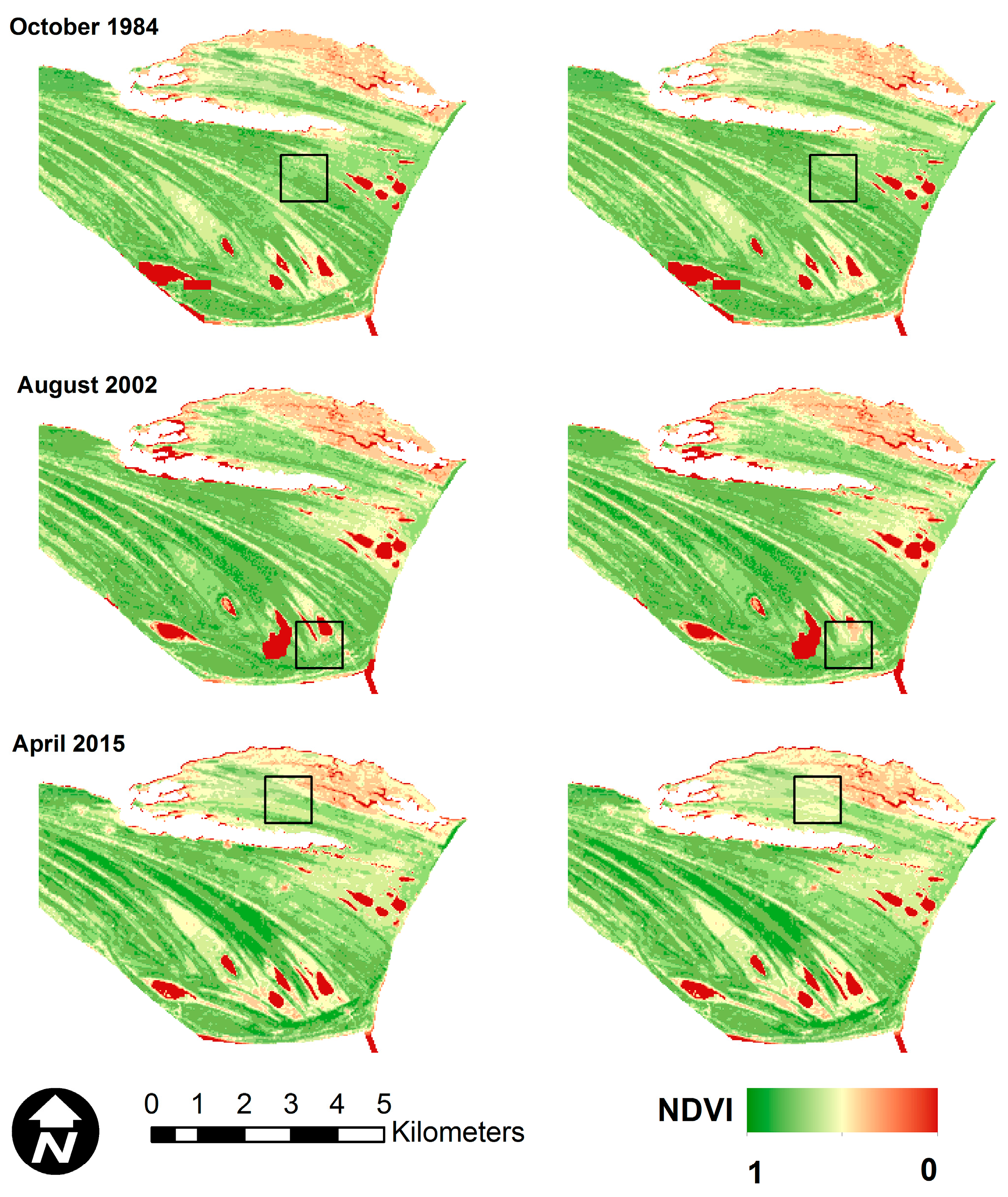
Figure 8.
Performance of OCPR on images with natural cloud cover (black). Areas to the southwest of the gray lines were not part of the area used to train the random forest model at the core of OCPR. All images are symbolized using the same color scale.
Figure 8.
Performance of OCPR on images with natural cloud cover (black). Areas to the southwest of the gray lines were not part of the area used to train the random forest model at the core of OCPR. All images are symbolized using the same color scale.


Table 1.
Description of existing methods to recover missing values from geospatial observations.
| Method | Advantages | Disadvantages |
|---|---|---|
| The Best Index Slope Extraction (BISE) [20,41] | Effective noise removal. | Dependence on threshold value and predefined time period; resulting profiles insensitive to timing of NDVI change. |
| Fourier based fitting [22] | Retain amplitude of local maxima and minima in time series. | Only determines overall curve shape, rather than identifying particular cycles; requires to rerunning over the entire time series every time new data are added. |
| Savitzy-golay (S-G) [5] | Preserves shape, timing and amplitude of time series for a broad range of phonologies. | Running mean and median filters alter the timing of local maxima and minima, even when weighted. |
| Asymmetric function fitting [41] | Preserves aesthetic value and geometric accuracy. | Successive relaxation of parameters depending on fit requires trial and error. |
| Nonlinear filter, ANN [42] | Computationally efficient; detects complex nonlinear relationships; multiple training algorithms including back propagation (BP) are supported. | “Black box” nature; tendency to over fit. |
| Multi-temporal regression | Efficient; applicable to small data sets. | Sensitive to outliers and can produce doubtful estimates for prediction. |
| Extreme learning machine [17] | Less training time compared to BP and SVM/SVR; outperforms BP in many applications. | Can over fit and get trapped in local minima. |
| Random Forest | No expectation of linear features; handles a wide range of training set sizes. | Tendency to over fit for regression when using limited, noisy data. |
Table 2.
Sample input data for training OCPR model.
| NDVI | Northing (m) | Easting (m) | Month | Rainfall (mm) | Temperature (°C) | Water Level (m) |
|---|---|---|---|---|---|---|
| 0.38 | 720,735 | 3,307,665 | 1 | 252.692 | 18.425 | 0.170 |
| 0.46 | 720,765 | 3,307,665 | 1 | 298.636 | 21.775 | 0.170 |
| 0.18 | 720,795 | 3,307,665 | 3 | 252.692 | 18.425 | 0.180 |
| 0.23 | 720,825 | 3,307,665 | 4 | 321.608 | 23.450 | 0.210 |
| 0.45 | 720,855 | 3,307,665 | 4 | 275.664 | 20.100 | 0.210 |
| 0.13 | 720,885 | 3,307,665 | 6 | 344.580 | 25.125 | 0.260 |
| 0.09 | 720,915 | 3,307,665 | 7 | 275.664 | 20.100 | 0.240 |
| 0.45 | 720,945 | 3,307,665 | 8 | 367.552 | 26.800 | 0.200 |
| 0.58 | 720,975 | 3,307,665 | 4 | 390.524 | 28.475 | 0.210 |
Table 3.
Sensitivity analysis of RF model using tree number and depth of tree.
| Tree Number | Tree Depth | RMSE | R2 |
|---|---|---|---|
| 10 | 12 | 0.0802 | 0.6987 |
| 12 | 12 | 0.0802 | 0.6989 |
| 22 | 12 | 0.0802 | 0.6985 |
| 35 | 12 | 0.0800 | 0.7001 |
| 60 | 12 | 0.0798 | 0.7023 |
| 120 | 12 | 0.0798 | 0.7017 |
| 10 | 30 | 0.0461 | 0.8949 |
| 12 | 30 | 0.0475 | 0.8944 |
| 22 | 30 | 0.0468 | 0.7017 |
| 35 | 30 | 0.0470 | 0.8951 |
| 60 | 30 | 0.0473 | 0.8946 |
| 120 | 30 | 0.0473 | 0.7018 |
| 10 | 60 | 0.0473 | 0.8949 |
| 12 | 60 | 0.0472 | 0.8955 |
| 22 | 60 | 0.0473 | 0.7025 |
| 35 | 60 | 0.0474 | 0.8967 |
| 60 | 60 | 0.0474 | 0.8973 |
| 120 | 60 | 0.0474 | 0.7040 |
| 500 | 12 | 0.0789 | 0.7017 |
| 500 | 30 | 0.0670 | 0.7018 |
| 500 | 60 | 0.0474 | 0.7040 |
| 500 | 60 | 0.0469 | 0.7052 |
Table 4.
Error metrics comparison between OCPR and Linear Regression.
| Method | RMSE | R2 |
|---|---|---|
| OCPR | 0.0162 | 0.9880 |
| LR | 0.1257 | 0.2596 |
Table 5.
Feature importance from the trained random forest model.
| Feature | Importance |
|---|---|
| Month | 0.034 |
| Easting (m) | 0.352 |
| Northing (m) | 0.492 |
| Rainfall (mm) | 0.039 |
| Temperature (°C) | 0.045 |
| Water Level (m) | 0.038 |
© 2017 by the authors. Licensee MDPI, Basel, Switzerland. This article is an open access article distributed under the terms and conditions of the Creative Commons Attribution (CC BY) license (http://creativecommons.org/licenses/by/4.0/).
Share and Cite
MDPI and ACS Style
Tahsin, S.; Medeiros, S.C.; Hooshyar, M.; Singh, A. Optical Cloud Pixel Recovery via Machine Learning. Remote Sens. 2017, 9, 527. https://doi.org/10.3390/rs9060527
AMA Style
Tahsin S, Medeiros SC, Hooshyar M, Singh A. Optical Cloud Pixel Recovery via Machine Learning. Remote Sensing. 2017; 9(6):527. https://doi.org/10.3390/rs9060527
Chicago/Turabian StyleTahsin, Subrina, Stephen C. Medeiros, Milad Hooshyar, and Arvind Singh. 2017. "Optical Cloud Pixel Recovery via Machine Learning" Remote Sensing 9, no. 6: 527. https://doi.org/10.3390/rs9060527
Note that from the first issue of 2016, this journal uses article numbers instead of page numbers. See further details here.