Article

Examination of the Potential of Terrestrial Laser Scanning and Structure-from-Motion Photogrammetry for Rapid Nondestructive Field Measurement of Grass Biomass

1
Geospatial Sciences Center of Excellence & Department of Geography, South Dakota State University, Brookings, SD 57007, USA
2
School for the Environment, University of Massachusetts Boston, Boston, MA 02125, USA
*
Author to whom correspondence should be addressed.
Remote Sens. 2017, 9(6), 531; https://doi.org/10.3390/rs9060531
Submission received: 4 April 2017 / Revised: 15 May 2017 / Accepted: 24 May 2017 / Published: 26 May 2017

Abstract

:
Above ground biomass (AGB) is a parameter commonly used for assessment of grassland systems. Destructive AGB measurements, although accurate, are time consuming and are not easily undertaken on a repeat basis or over large areas. Structure-from-Motion (SfM) photogrammetry and Terrestrial Laser Scanning (TLS) are two technologies that have the potential to yield precise 3D structural measurements of vegetation quite rapidly. Recent advances have led to the successful application of TLS and SfM in woody biomass estimation, but application in natural grassland systems remains largely untested. The potential of these techniques for AGB estimation is examined considering 11 grass plots with a range of biomass in South Dakota, USA. Volume metrics extracted from the TLS and SfM 3D point clouds, and also conventional disc pasture meter settling heights, were compared to destructively harvested AGB total (grass and litter) and AGB grass plot measurements. Although the disc pasture meter was the most rapid method, it was less effective in AGB estimation (AGBgrass r2 = 0.42, AGBtotal r2 = 0.32) than the TLS (AGBgrass r2 = 0.46, AGBtotal r2 = 0.57) or SfM (AGBgrass r2 = 0.54, AGBtotal r2 = 0.72) which both demonstrated their utility for rapid AGB estimation of grass systems.

Graphical Abstract

1. Introduction

Quantification of the above ground biomass (AGB, units g m−2) of grasslands is important for a number of applications including pasture management [1], wildlife habitat monitoring [2,3], fire management [4,5], carbon storage [6,7], and understanding the implications of biophysical and ecological processes that influence grass production [8,9]. Destructive methods of AGB estimation require cutting, drying, and weighing grass samples, which is time consuming, inefficient for large area application, and may preclude repeat temporal estimation as the grass is physically removed. Conventional grassland AGB estimation methods rely on allometric relationships established between destructively harvested AGB plot data and a grass structural property, such as the grass height, that can be measured elsewhere [10,11]. For example, a long established grass AGB estimation method is the disc pasture meter which allometrically relates the settling height of a weighted disc on a grassland plot to the AGB beneath it [12,13].
Recent technological advances in active and passive remote sensing have potential for rapid grass AGB estimation. Terrestrial Laser Scanning (TLS) provides a ground based way to estimate the biomass of trees and shrubs. Three dimensional (3D) point clouds of the vegetation surface are derived from laser scans and allow the reconstruction of quantitative 3D vegetation models [14,15,16] that, with knowledge of the vegetation density, enable biomass estimation without allometric information [17,18]. Most TLS studies have focused on woody vegetation, although studies have used TLS for assessing grass height, including the change in height associated with grazing [19] and fire [20,21], as well as for estimating the AGB of crops [22,23]. A limited number of studies have used TLS to estimate grass biomass. For example, Umphries [24] related TLS height metrics over bunchgrass to destructively harvested AGB, obtaining r2 values ranging from 0.30 to 0.42. Eitel et al. [25] used TLS volume estimates to derive the AGB of winter wheat over two growing seasons (r2 > 0.72). Schaefer and Lamb [26] used TLS derived grass height and the normalized difference vegetation index (NDVI) to estimate tall fescue biomass and found that together they produced better estimates (r2 = 0.76) than using only the TLS height (r2 = 0.61) or only the NDVI (r2 = 0.56).
Structure-from-Motion (SfM) is used to generate 3D point clouds from overlapping 2D photographs using photogrammetric and computer vision techniques [27]. The primary application of SfM has been on the analysis of topography [28,29] and man-made features [30,31]. Improved digital camera technology and computing capabilities enable rapid SfM implementation. SfM has been used to estimate tree heights and stem diameters [32,33,34,35], tree volumes [36,37], shrub heights [38], and crop heights [39,40,41]. However, no studies to our knowledge have used SfM to assess grass biomass. This is perhaps because non-crop grasses are often irregular which may reduce the efficacy of point cloud generation using SfM image matching procedures.
This study examines the potential of TLS and SfM photogrammetry for rapid nondestructive estimation of grass AGB. Eleven grass plots selected over a range of biomass from about 150 g m−2 to 1050 g m−2 in South Dakota, USA, were measured using a TLS and a digital camera. Volume metrics extracted from the 3D point clouds, and also disc pasture meter settling heights, were compared to destructively harvested AGB measurements. An assessment of the practical limitations of each method and recommendations for future research are discussed.

2. Materials and Methods

2.1. Study Area and Grass Plots

Field measurements were collected at the North Farm Unit of Oak Lake Field Station, Eastern South Dakota in September and October 2016. The field station has been affiliated with South Dakota State University since 1988 and the North Farm Unit has been left without human management since then. The field station is located on the Northern Glaciated Plains and has a mid-continental climate with a mean annual precipitation of 58 cm, the majority occurring before August, and a mean annual temperature of 5.9 °C [42].
Eleven 1 × 1 m plots were selected to encompass a range of likely grass AGB by selecting plot locations with a range of grass heights from approximately 50 to 70 cm. Only plots containing the invasive cool season Smooth Brome (Bromus inermis) grass were selected. The grass was partially senescent and each plot contained dead litter understory. The grass blades were typically less than 1 mm thick and less than 1 cm wide and oriented in many directions. Each plot included a minority of seed heads on millimeter stems with heights varying from 90 to 120 cm. All the plots were on relatively flat (<5° inclination) sites on well drained, fine-loamy soils in the Singsass-Buse soil complex [43].
Each plot was delineated by four 1.2 m tall vertical poles that were 0.8 cm in diameter (Figure 1). The poles were covered in red fluorescent plastic with a white reflective band that had notably higher TLS return intensities, and also could be clearly discerned in the digital photographs. After each pole was placed into the ground the distance from the bottom of the white reflective band to the soil at the pole base was measured using a tape measure. In addition, a painted cube target was placed on top of each pole to help align the digital photographs.

2.2. Data Collection

2.2.1. Remotely Sensed Data Measurement

The compact biomass LiDAR (CBL), built by the University of Massachusetts Boston, is a new generation of TLS that is inexpensive and optimized for rapid scanning and portability [44]. It uses a SICK LMS151 LiDAR and records the first and last returns at 905 nm over a 360° horizontal and 270° vertical scan in less than 35 s. It has a 0.25° angular resolution and a 0.86° beam divergence and a maximum range of 40 m. The CBL was placed on a tripod and oriented with a level so that the resulting x, y point cloud was in the horizontal plane. Four CBL scans were taken from opposing sides of each plot to minimize occlusion [45,46]. For each scan, the CBL was placed 1.6 m from the side of the plot at a height of 1.6 m. This ensured that the CBL was always above the grass (heights 50 to 70 cm) and meant that the grass was between 1.84 m and 2.80 m away from the CBL. At these ranges, the LiDAR pulses are sensed every 0.80 to 1.22 cm with pulse widths of 2.76 cm to 4.20 cm. All the CBL scans were acquired on windless days to minimize vegetation movement.
A Canon EOS 6D 20 Megapixel digital single-lens reflex camera was used to take true color digital images of each plot. A Canon EF 24–70 mm f/4L IS USM lens was used. The lens coatings provide improved color rendering and minimal ghosting compared to more standard lenses and are resistant to dust and water. The lens is stabilized and has low dispersion aspherical detector elements to minimize chromatic and spherical aberration and color blurring around subject edges. Approximately 150 overlapping digital images were taken by hand in concentric circles 1.5 m from the center of each plot. Several passes were made at varying heights so that a full hemispherical coverage was obtained. The large number of photographs ensured that they were spatially overlapping by more than 50% horizontally and vertically and so they could be used in the SfM image matching process. The camera parameters were manually selected based on the ambient light conditions. Specifically, the ISO settings were kept low to reduce sensitivity to light and to provide finer grain digital photographs, while keeping a small aperture size but adequate shutter speed so that sharp images with low noise were captured. It took approximately 10 min to take all of the photographs for one plot. The photographs were taken under consistent solar conditions (either overcast or clear skies) to reduce unhelpful variation in lighting conditions [36].

2.2.2. Disc Pasture Meter Measurement

A disc pasture meter was used after the remotely sensed data were collected. A vertical pole and a weighted 0.46 m × 0.46 m square disc that is not in contact with the pole, with specifications described in [47], was placed onto the grass at the center of each plot. The disc settling height was measured to the nearest millimeter using a rule etched onto the pole.

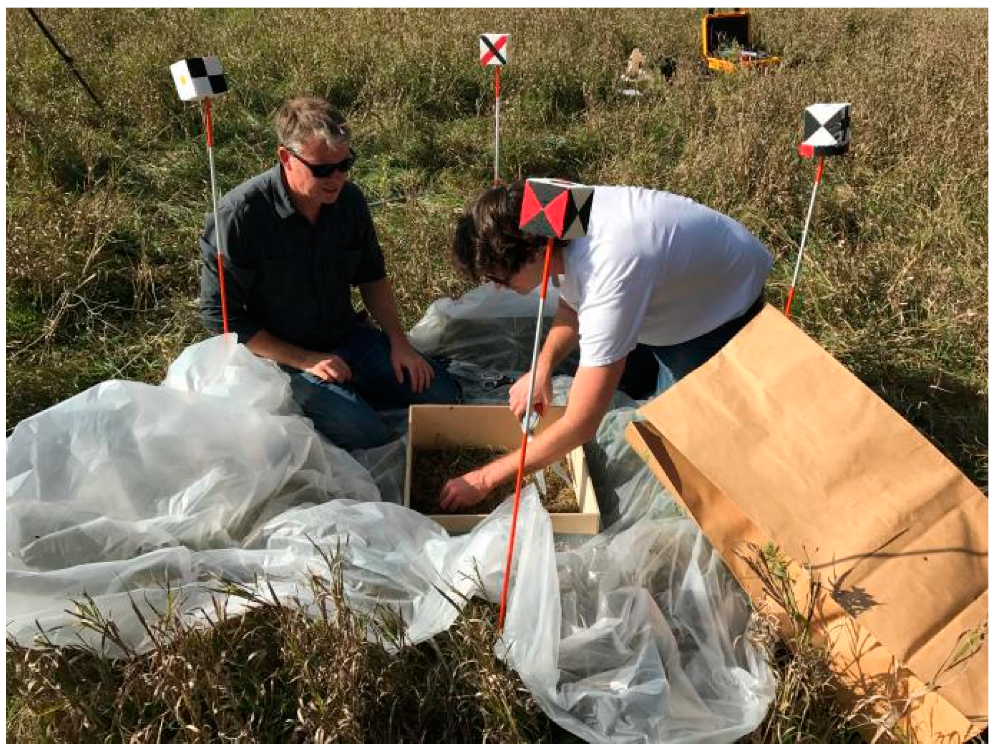
2.2.3. Destructive Grass Harvesting

After the above measurements, the grass and litter was removed manually from each plot. A wooden frame that encompassed the 0.46 m × 0.46 m disc pasture meter was placed at the plot center and all the standing grass material within the frame was removed (Figure 1). In each plot there was always a non-negligible litter layer at the bottom of the grass stems. The litter was removed and bagged separately from the grass.

2.3 Remotely Sensed Data Analysis

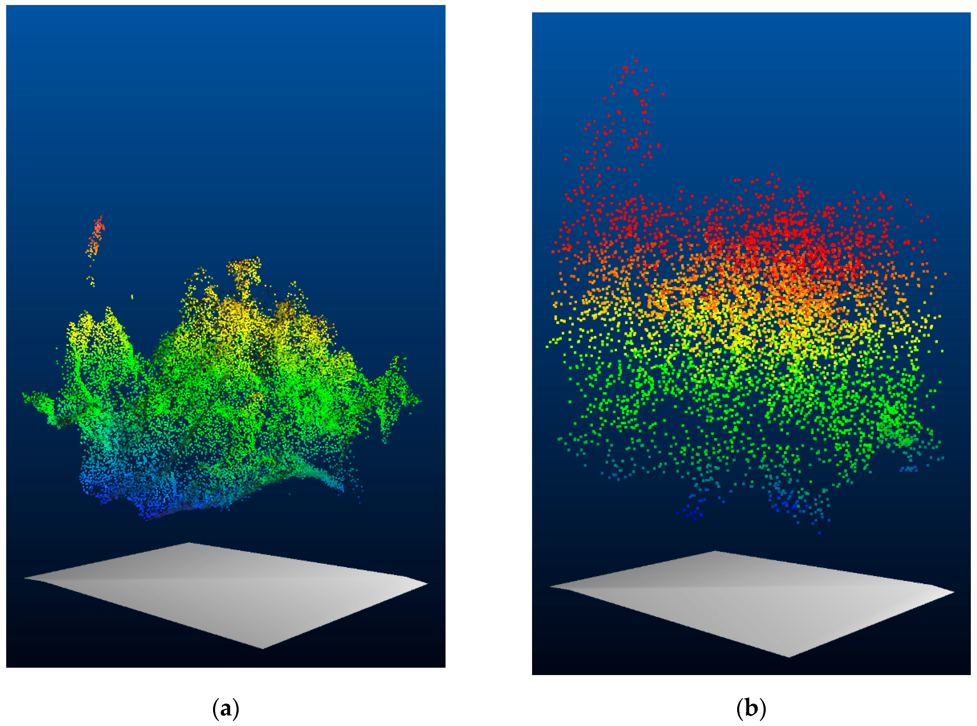
2.3.1. Pre-Processing–Aligned 3D Point Cloud Generation

The four CBL scans (composed of x, y, z coordinates and LiDAR intensities) were combined using the recent Version 2.7.0 CloudCompare software [48]. In each scan, the four poles were apparent and so the four scans were aligned interactively using the LiDAR first returns from the poles, and in particular using the returns from the tops and bottoms of the white reflective bands, which were quite evident due to their higher return intensities.
The digital photographs were processed using the recent Version 1.2.5 Agisoft Photoscan Pro SfM software [49] running on a high performance Linux server (64 cores with 512 GB RAM). Shadows cast by the photographer were first manually masked from each photograph. Then the photographs were aligned and the camera orientations derived automatically by matching features common to the overlapping photographs using the Photoscan Pro software. The feature matching was difficult due to the homogenous and repetitive appearance of the grass. Consequently the alignment accuracy parameter—which could be set as ‘lowest’, ‘low’, ‘medium’, ‘high’, or ‘highest’—was set to ‘low’. Using a higher accuracy setting resulted in large gaps in the point cloud. The matched point coordinates were output to provide a sparse 3D point cloud. A dense, high quality 3D point cloud was then generated using mild depth filtering to automatically remove erroneous points from the dense point cloud (e.g., points estimated below the ground surface).
The resulting SfM and TLS point clouds were aligned interactively using CloudCompare. Specifically, for each plot, the SfM point cloud was aligned to the TLS point cloud, taking advantage of the evident poles. The aligned point clouds were spatially clipped to a 0.5 m × 0.5 m area centered on the plot center.

2.3.2. Pre-Processing—Ground Surface Estimation

Although the plots were on flat (<5°) sites, a planar model of the ground surface was defined. The x, y, z coordinates of the bottoms of the white reflective bands on each pole were identified in the aligned 3D point clouds. Then the measured distances from the bottoms of the white reflective bands to the ground surface (Section 2.1) were subtracted from each z coordinate. This yielded four x, y, z coordinates defining the location of the ground at the base of each pole relative to the point clouds. The ground surface was defined by two 3D triangles with vertices defined by the pole base x, y, z coordinates.

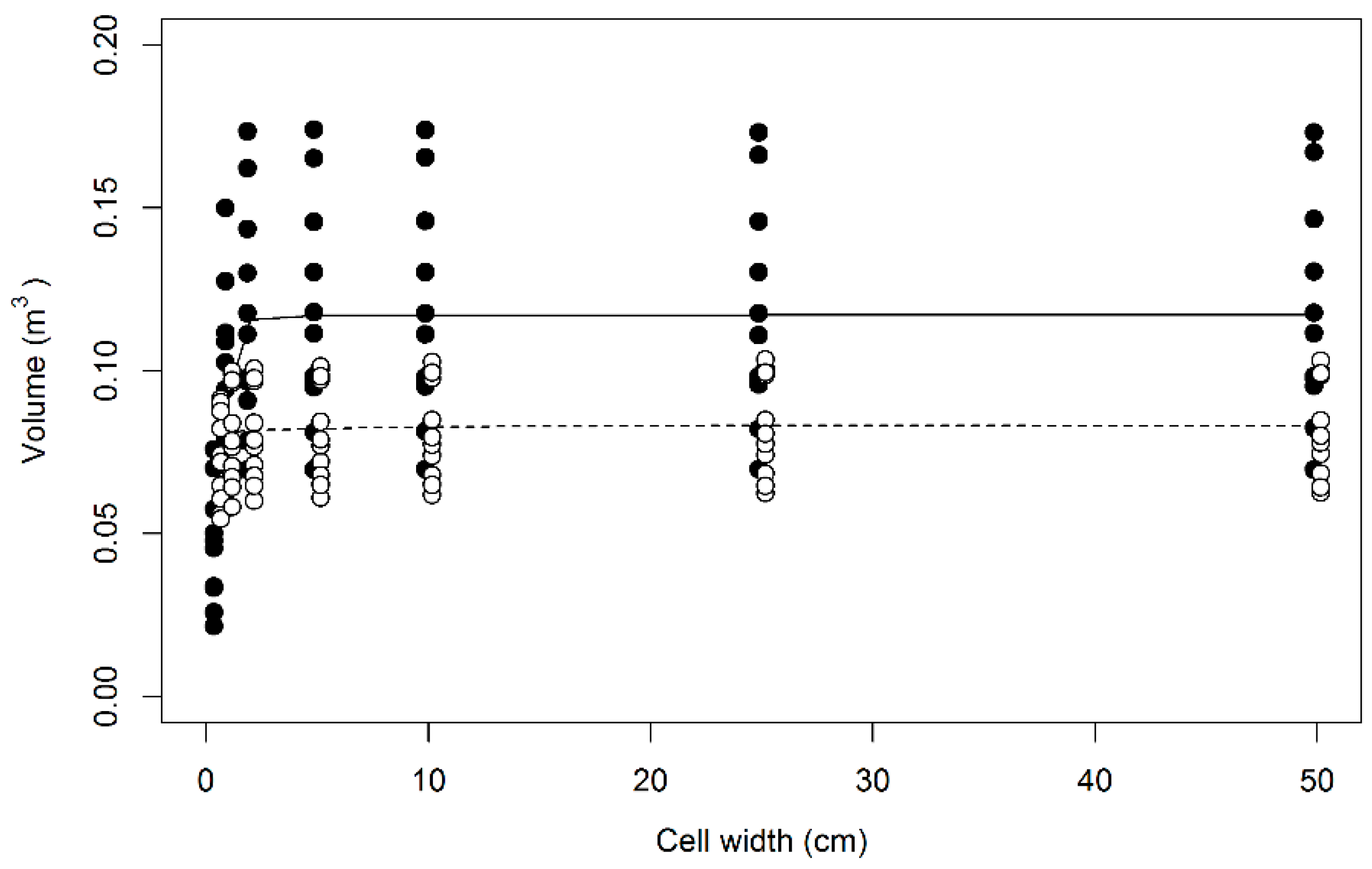
2.3.3. Grass Volume Estimation

The volume of the grass including litter (that could not be separately resolved with the TLS or SfM data) was derived from the aligned 3D point clouds using a volumetric surface differencing approach. Established voxel counting methods, which involve partitioning the point cloud into voxels and then counting the number of voxels containing at least one point [50,51], were not used as they require full canopy penetration, which was not obtained due to the close packed nature of the grasses. Similarly, more sophisticated volume estimation methods based on derivation of quantitative 3D vegetation models [15] were inappropriate as the grass structural components could not be resolved in the point clouds.
The volumetric surface differencing approach does not require full canopy penetration but implicitly assumes that the space beneath the points to the ground surface are occupied by vegetation [25,52,53]. First, the z coordinate of each point was converted into a height above the ground to account for site topography [54]. This was undertaken by subtracting the interpolated ground surface planar model z value at the point cloud x, y location from the corresponding point cloud z coordinate. Then the point clouds were partitioned in the x, y plane into square cells. The mean height of all the points falling within each of the cells was calculated. The cell grass volume was estimated as the product of the mean height and the cell side dimensions. The total grass volume (m3) was calculated by summing the volumes of all the cells within the 0.5 m × 0.5 m point cloud.
The point cloud derived grass volume estimation was expected to be sensitive to the cell dimensions used [52]. To investigate this, the grass volumes were estimated considering a range of cell dimensions (0.5, 1, 2, 5, 10, 25, and 50 cm). A minimum 0.5 cm cell dimension was used as it is smaller than the 0.80 to 1.22 cm spatial sampling provided by the CBL configuration (Section 2.2.1). The largest 50 cm cell dimension was used, as the resulting volume estimate is equivalent to the mean point cloud height, which has been used by previous researchers [24,26], multiplied by the 0.5 m × 0.5 m point cloud area.

2.4. Destructively Harvested AGB Grass and Litter Estimation

The destructively harvested grass and litter for each plot were dried separately in an oven at 60 °C for 72 h and then weighed with an accurate laboratory scale. The dry weight of the grass and litter, and the weight of the grass alone, were converted to AGB (units g m−2) by dividing by 0.46 × 0.46 to provide AGBtotal and AGBgrass estimates respectively for each plot.

2.5. Remotely Sensed and Disc pasture Meter AGB Grass and Litter Estimation
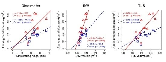
The volume measurements derived from TLS and SfM point clouds, as well as the settling height of the disc pasture meter, were related to the destructively harvested AGBtotal and AGBgrass estimates for the 11 plots using ordinary least squares (OLS) linear regression. The OLS regression goodness of fit (r2) and F-test p-value were used to measure correspondence between these data.
To compare the AGB predictive capability of the regression models, a boot-strapped ‘leave-one-out’ model cross-validation approach was undertaken considering the AGBtotal and AGBgrass and the TLS, SfM, and disc pasture meter plot data. Specifically, 11 OLS regressions were generated, each time leaving out one plot for model validation and using the remaining 10 plots to generate the regression. The following quantities were derived
r e s i d u a l i =   A G B i   A G B ^
R M S E = i = 1 11 r e s i d u a l i 2 11
where r e s i d u a l i is the difference between the harvested AGB for the ‘left out’ plot i ( A G B i ) and the predicted AGB ( A G B ^ ) derived using the OLS regression parameters defined using the data for the 10 other plots, and the RMSE is the root mean square error of the eleven r e s i d u a l i values.

3. Results

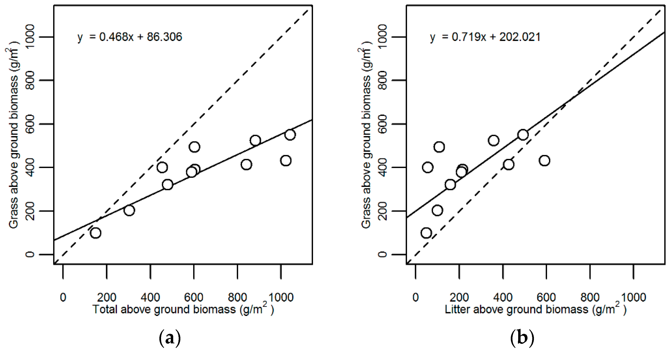
3.1. Destructively Harvested AGB

Among the 11 plots the destructively harvested AGB for grass (AGBgrass) varied from 99.5 g/m2 to 551 g/m2 (mean 382.7 g/m2) and for grass and litter (AGBtotal) varied from 149 g/m2 to 1043 g/m2 (mean 634.03 g/m2) (Figure 2).
The range of destructively harvested AGB values is comparable to that found in other undisturbed grass systems [55] including smooth brome pastures [56]. The amount of litter biomass was directly proportional to AGBgrass and AGBtotal and varied from 49.13 g/m2 to 590.87 g/m2. The relatively high litter biomass was likely because the study site was not mown or grazed by domestic animals, or subject to prescribed fires, for at least two decades.

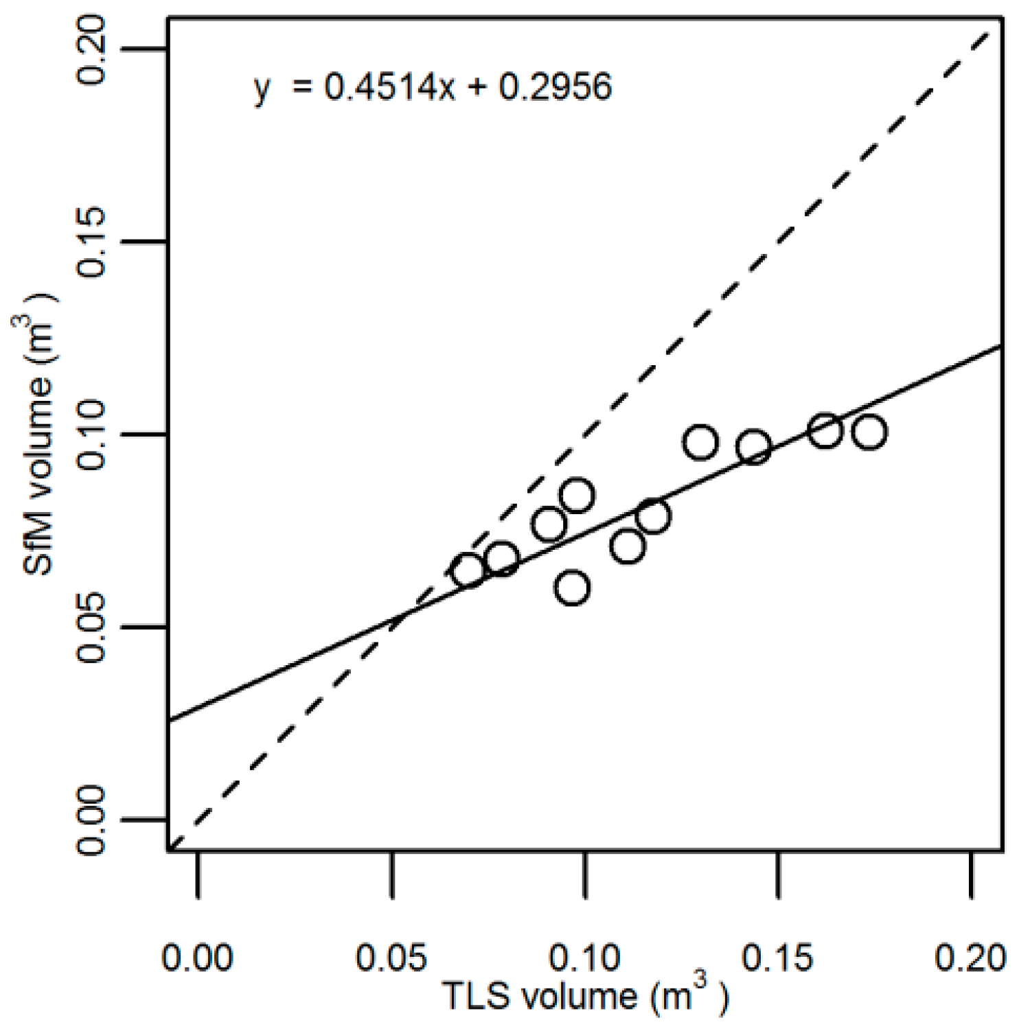
3.2. Point Cloud Grass Volumes

The SfM and TLS 3D point clouds were morphologically similar but with evident differences (Figure 3). For all 11 plots, including those with the lowest AGB, neither the SfM nor the TLS provided canopy penetration to the ground or to the litter layer. The SfM point clouds had a greater density of points (typically 40,000 points per 0.5 m × 0.5 m plot) compared to the TLS point clouds (typically 5000 points per plot). Within the main vegetation canopy, more structural detail was visually apparent in the SfM point clouds. However, some of the isolated elements at the top of the canopy (taller grass blades and seed heads) were not present in the SfM point cloud due the SfM depth filtering (although minimal, this filtering was not disabled as without it a minority of noisy mismatched points remained that rendered the point cloud unusable). More of the elements at the top of the canopy were captured by the TLS because the LiDAR pulse width was larger than most of the grass blades and they were captured as partial LiDAR returns. Thus, although certain isolated seed heads and grass blades are more apparent in Figure 3a than in Figure 3b, more of the canopy top is apparent in Figure 3b.
The point cloud derived plot volume estimates were quite similar when derived using cell dimensions greater than 0.5 cm × 0.5 cm with the SfM volumes typically 27% less than the TLS volumes (Figure 4). The plot volumes estimated with a 0.5 cm × 0.5 cm cell dimension were markedly lower than for the other cell dimensions and occurred because some 0.5 cm × 0.5 cm cells contained no points. With cell dimensions of 2.0 cm × 2.0 cm there were always points within each cell for the TLS or SfM point clouds. The remainder of the analyses were carried out using point cloud volumes derived with 2 cm cell dimensions.
Figure 5 Illustrates in detail the SfM and TLS volumes for the 11 plots derived using a 2.0 cm × 2.0 cm cell dimension. The SfM volumes have a smaller range (from 0.0602 to 0.0817 m3) than the TLS volumes (from 0.0698 to 0.1736 m3). Despite this, the TLS and SfM volumes are well correlated (r = 0.76), indicating that both remote sensing methods provide related results.

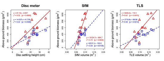
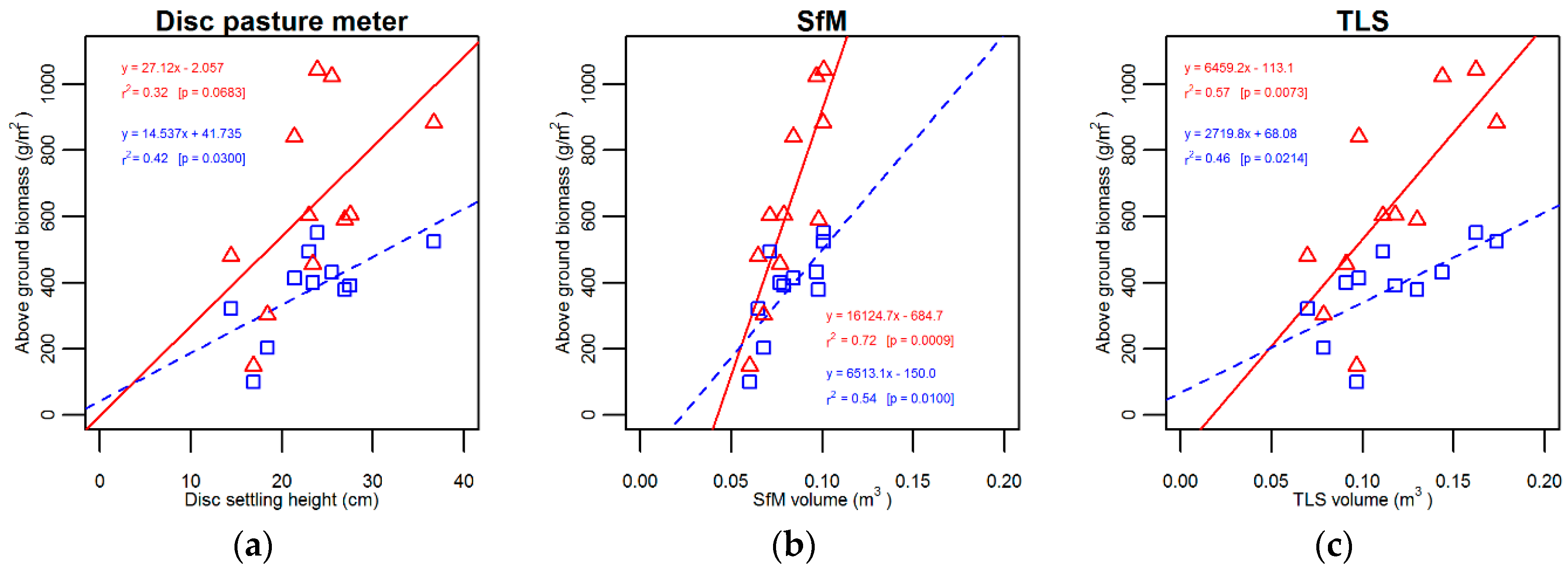
3.3. Remotely Sensed and Disc Pasture Meter AGB Estimation

The destructively harvested above ground biomass data were compared by OLS regression with the disc pasture meter settling heights and with the plot volumes derived from the SfM and TLS point clouds (Figure 6). Considering the regression goodness of fit (r2), a clear pattern emerges for the three AGB estimation methods.
The disc pasture meter settling heights had the least correspondence with the harvested AGB. The settling height has better correspondence with AGBgrass (r2 = 0.42) than with AGBtotal (r2 = 0.32). However, the regressions were not particularly significant (AGBtotal p = 0.068 and AGBgrass p = 0.030).
The volumes derived from the SfM point clouds had the highest correspondence with the harvested AGB, both for AGBtotal (r2 = 0.72) and AGBgrass (r2 = 0.54). The TLS volumes provided relatively lower correspondence for both AGBtotal (r2 = 0.57) and AGBgrass (r2 = 0.46). For both data types, the volume estimates corresponded better with AGBtotal than with AGBgrass.
The results of the ‘leave-one-out’ model cross validation are summarized in Table 1. The RMSE values indicate that the disc pasture meter settling height data provided poor predictive capability with RMSE values of 120.1 g/m2 (AGBgrass) and 268.7 g/m2 (AGBtotal). These errors are quite large, and correspond to 31% and 42% of the means of the destructively harvested AGBgrass and AGBtotal plot data respectively (Figure 2).
The point cloud based methods provided improved AGB predicative capability compared to the disc pasture meter method (Table 1). The SfM RMSE values were smaller than the TLS RMSE values although there was marginal difference between the AGBgrass RMSE values (approximately 109 g/m2 that corresponds to about 28% of the mean of the destructively harvested AGBgrass plot data). The SfM and TLS AGBtotal RMSE values (178.8 g/m2 and 215.3 g/m2) correspond to 28% and 34% of the mean of the destructively harvested AGBtotal plot data respectively.

4. Discussion

The disc pasture meter provided the least accurate method for AGB estimation, with the lowest r2 (Figure 6) and highest AGB predictive RMSE values (Table 1). The settling height had better correspondence with AGBgrass (r2 = 0.42) than with AGBtotal (r2 = 0.32). This may be because the litter resided at the bottom of the grass stems and so had little influence on the grass mechanical strength and therefore on the disc settling height. The correspondence between the disc pasture meter settling heights and the destructively harvested AGB described in this study were lower than reported in some literature, which may be due to site and grass differences [12,57].
Neither the SfM nor the TLS data provided canopy penetration to the litter layer or to the ground surface due to the dense packing of the grass. Consequently, a volumetric surface differencing approach was used to derive grass volumes from the 3D point clouds. This method implicitly assumes that the space beneath the points to the ground surface are occupied by vegetation [25,52,53]. Neither the TLS nor SfM volume estimates were sensitive to the cell dimension used when all the cells contained point cloud data. While this sensitivity is expected to vary with the vegetation structure and the instrumentation, this suggests that using mean height point cloud metrics, at least for the grasses considered in this study, is sufficient for relating point cloud metrics to grass AGB e.g., [26].
The SfM derived grass volumes were correlated with the TLS derived volumes but were typically 27% smaller and defined over a narrower range of values (Figure 4 and Figure 5). This is likely because, although the SfM point clouds captured more detail within the main canopy, the TLS captured more of the isolated elements of the canopy top (single glass blades and seed heads) (Figure 3). The comparatively wide TLS beam divergence (0.86°) may have resulted in relatively more captured isolated vegetation elements but with a commensurate reduction in the localization accuracy of the returns. In terms of the volume estimation method, this could misplace returns into multiple cells, resulting in a relative overestimation of the volume. If the SfM and TLS measurements were taken closer or further away from the grass then the interplay of these factors may change.
The SfM photogrammetry volumetric surface differencing approach provided the most accurate method for AGB estimation. The volumes derived from the SfM point clouds had higher correspondence with the harvested AGB than the TLS point clouds and had r2 values comparable to other studies [25,26]. Interestingly, both the SfM and TLS volume estimates had higher correspondence with the harvested AGBtotal than with the harvested AGBgrass data (Figure 6). Neither the SfM nor the TLS resolved the litter, which increased with AGBgrass and with AGBtotal (Figure 2). Consequently, the difference between AGBtotal and AGBgrass was greater for the higher biomass plots but the point cloud derived volumes were the same (Figure 6). This is also why there was only a marginal difference between the SfM and TLS AGBgrass RMSE values but distinct differences between the SfM and TLS AGBtotal RMSE values (Table 1). The SfM photogrammetry approach provided better AGBtotal predictive capability than the TLS.
The different AGB estimation methods considered in this study have quite different practical limitations. The disc pasture meter method is straightforward and rapid, as it takes only seconds to place and measure the disc settling height, and it is the least expensive of the three methods. Furthermore, unlike the other methods, it can be undertaken on windy days. However, it is the least accurate. The CBL is a new generation of TLS that is inexpensive and optimized for rapid scanning and portability [44]. It took less than 10 min to set up and complete the four CBL scans for each plot. A similar amount of time was spent taking the approximately 150 digital photographs per plot. However, the processing required to generate 3D point clouds was markedly different between the TLS and SfM methods, typically 30 min per plot for the TLS data and five times more for the SfM data due to greater computer processing requirements. Although the CBL is more expensive than a digital camera it does not require a high performance computer to process the collected data. The TLS processing could be undertaken on a laptop computer in the field but except for generating ‘quick look’ images this was not considered an advantage due to the difficulty of operating a laptop in natural daylight.
Further work to assess the impact of confounding factors on AGB estimation using TLS and SfM derived measurements is recommended. Such factors include sensitivity to grass species composition, growth stage, structure and condition, seasonality, and the amount of litter. The failure of point clouds to capture the extremities of fine scale vegetation is well known and is due to numerous factors, particularly those related to the ability to resolve vegetation elements, match elements in the point clouds, and the implementation of appropriate point cloud filtering. Further research to investigate these aspects is recommended. It may be possible to combine SfM and TLS point clouds to provide improved AGB estimates but again further research is required. Finally, we note that both technologies have potential for upscaling AGB estimates from plot-level measurements to field-level measurements using terrestrial vehicle or airborne platforms.

5. Conclusions

The results of this study demonstrate the potential of SfM photogrammetry and TLS for nondestructive estimation of grass AGB. The study was limited to one type of grass and may not be transferable to other species and types. Despite being more rapid, the established disc pasture meter was found to be the least accurate of the three methods considered. The disc pasture meter settling height had poor correspondence with harvested AGBtotal (r2 = 0.32) and AGBgrass (r2 = 0.42). The SfM photogrammetry approach provided more accurate estimation of AGBtotal and AGBgrass than the TLS or disc pasture meter approaches. The SfM and TLS volume estimates had higher correspondence with harvested AGBtotal (r2 = 0.72 and r2 = 0.57) than with harvested AGBgrass data (r2 = 0.54 and r2 = 0.46) due primarily to the inability of SfM and TLS measurements to resolve the litter layer. A volumetric surface differencing approach was used to derive grass volumes from the 3D point clouds but there was little observed sensitivity to the cell dimension used. Further research to determine the major influencing factors and to establish optimal methodologies for SfM and TLS data acquisition in grassland ecosystems is recommended. Each method has different practical limitations, and the results of this study suggest that selecting a particular method should be influenced by accuracy and application requirements.

Acknowledgments

This research was funded by a South Dakota State University (SDSU) Geospatial Sciences Center of Excellence Research Assistantship. Sanath Sathyachandran Kumar is thanked for helping with the field measurements and Francesco Peri is thanked for technical assistance with the Compact Biomass LiDAR.

Author Contributions

S.C. and D.R. conceived the experiments; S.C. collected and processed the data, undertook the data analysis, and developed the graphics, D.R. helped with the data analysis and structured and drafted the manuscript with assistance from I.P., S.C., and C.S.

Conflicts of Interest

The authors declare no conflict of interest.

References

  1. Trotter, M.G.; Lamb, D.W.; Donald, G.E.; Schneider, D.A. Evaluating an active optical sensor for quantifying and mapping green herbage mass and growth in a perennial grass pasture. Crop Pasture Sci. 2010, 61, 389–398. [Google Scholar] [CrossRef]
  2. McNaughton, S. Ecology of a grazing ecosystem: The serengeti. Ecol. Monogr. 1985, 55, 259–294. [Google Scholar] [CrossRef]
  3. Carlyle, C.N.; Fraser, L.H.; Haddow, C.M.; Bings, B.A.; Harrower, W. The use of digital photos to assess visual cover for wildlife in rangelands. J. Environ. Manag. 2010, 91, 1366–1370. [Google Scholar] [CrossRef] [PubMed]
  4. Trollope, W.S.W.; Trollope, L.A.; Potgieter, A.F.L.; Zambatis, N. Safari-92 characterization of biomass and fire behavior in the small experimental burns in the Kruger National Park. J. Geophys. Res. Atmos. 1996, 101, 23531–23539. [Google Scholar] [CrossRef]
  5. Kauffman, J.B.; Cummings, D.L.; Ward, D.E. Relationships of fire, biomass and nutrient dynamics along a vegetation gradient in the Brazilian Cerrado. J. Ecol. 1994, 82, 519–531. [Google Scholar] [CrossRef]
  6. Tilman, D.; Hill, J.; Lehman, C. Carbon-negative biofuels from low-input high-diversity grassland biomass. Science 2006, 314, 1598–1600. [Google Scholar] [CrossRef] [PubMed]
  7. Scurlock, J.M.O.; Hall, D.O. The global carbon sink: A grassland perspective. Glob. Chang. Biol. 1998, 4, 229–233. [Google Scholar] [CrossRef]
  8. Loreau, M.; Hector, A. Partitioning selection and complementarity in biodiversity experiments. Nature 2001, 412, 72–76. [Google Scholar] [CrossRef] [PubMed]
  9. Tilman, D.; Reich, P.B.; Knops, J.; Wedin, D.; Mielke, T.; Lehman, C. Diversity and productivity in a long-term grassland experiment. Science 2001, 294, 843–845. [Google Scholar] [CrossRef] [PubMed]
  10. Evans, R.A.; Jones, M.B. Plant height times ground cover versus clipped samples for estimating forage production. Agron. J. 1958, 50, 504–506. [Google Scholar] [CrossRef]
  11. Williamson, S.C.; Detling, J.K.; Dodd, J.L.; Dyer, M.I. Nondestructive estimation of shortgrass aerial biomass. J. Range Manag. 1987, 40, 254–256. [Google Scholar] [CrossRef]
  12. Santillan, R.A.; Ocumpaugh, W.; Mott, G. Estimating forage yield with a disk meter. Agron. J. 1979, 71, 71–74. [Google Scholar] [CrossRef]
  13. Holmes, C. The massey grass meter. In Dairy Farming Annual; Massey University: Palmerston North, New Zealand, 1974; pp. 26–30. [Google Scholar]
  14. Kaasalainen, S.; Krooks, A.; Liski, J.; Raumonen, P.; Kaartinen, H.; Kaasalainen, M.; Puttonen, E.; Anttila, K.; Makipaa, R. Change detection of tree biomass with terrestrial laser scanning and quantitative structure modelling. Remote Sens. 2014, 6, 3906–3922. [Google Scholar] [CrossRef]
  15. Raumonen, P.; Kaasalainen, M.; Akerblom, M.; Kaasalainen, S.; Kaartinen, H.; Vastaranta, M.; Holopainen, M.; Disney, M.; Lewis, P. Fast automatic precision tree models from terrestrial laser scanner data. Remote Sens. 2013, 5, 491–520. [Google Scholar] [CrossRef]
  16. Cote, J.F.; Fournier, R.A.; Egli, R. An architectural model of trees to estimate forest structural attributes using terrestrial LiDAR. Environ. Model. Softw. 2011, 26, 761–777. [Google Scholar] [CrossRef]
  17. Calders, K.; Newnham, G.; Burt, A.; Murphy, S.; Raumonen, P.; Herold, M.; Culvenor, D.; Avitabile, V.; Disney, M.; Armston, J.; et al. Nondestructive estimates of above-ground biomass using terrestrial laser scanning. Methods Ecol. Evol. 2015, 6, 198–208. [Google Scholar] [CrossRef]
  18. Dassot, M.; Constant, T.; Fournier, M. The use of terrestrial LiDAR technology in forest science: Application fields, benefits and challenges. Ann. For. Sci. 2011, 68, 959–974. [Google Scholar] [CrossRef]
  19. Radtke, P.J.; Boland, H.T.; Scaglia, G. An evaluation of overhead laser scanning to estimate herbage removals in pasture quadrats. Agric. For. Meteorol. 2010, 150, 1523–1528. [Google Scholar] [CrossRef]
  20. Rowell, E.; Seielstad, C. Characterizing grass, litter, and shrub fuels in longleaf pine forest pre-and post-fire using terrestrial LiDAR. In Proceedings of the SilviLaser, Vancouver, BC, Canada, 16–19 September 2012. [Google Scholar]
  21. Wallace, L.; Gupta, V.; Reinke, K.; Jones, S. An assessment of pre-and post fire near surface fuel hazard in an Australian dry sclerophyll forest using point cloud data captured using a terrestrial laser scanner. Remote Sens. 2016, 8, 679. [Google Scholar] [CrossRef]
  22. Tilly, N.; Hoffmeister, D.; Cao, Q.; Huang, S.; Lenz-Wiedemann, V.; Miao, Y.; Bareth, G. Multitemporal crop surface models: Accurate plant height measurement and biomass estimation with terrestrial laser scanning in paddy rice. J. Appl. Remote Sens. 2014, 8, 083671. [Google Scholar] [CrossRef]
  23. Hütt, C.; Schiedung, H.; Tilly, N.; Bareth, G. Fusion of high resolution remote sensing images and terrestrial laser scanning for improved biomass estimation of maize. Int. Arch. Photogram. Remote. Sens. Spat. Inf. Sci. 2014, 40, 101. [Google Scholar] [CrossRef]
  24. Umphries, T.A. Characterizing Fuelbed Structure, Depth, and Mass in a Grassland Using Terrestrial Laser Scanning. Master’s Thesis, University of Montana, Missoula, MT, USA, 2013. [Google Scholar]
  25. Eitel, J.U.H.; Magney, T.S.; Vierling, L.A.; Brown, T.T.; Huggins, D.R. LiDAR based biomass and crop nitrogen estimates for rapid, non-destructive assessment of wheat nitrogen status. Field Crop. Res. 2014, 159, 21–32. [Google Scholar] [CrossRef]
  26. Schaefer, M.T.; Lamb, D.W. A combination of plant NDVI and LiDAR measurements improve the estimation of pasture biomass in tall fescue (Festuca arundinacea var. Fletcher). Remote Sens. 2016, 8, 109. [Google Scholar] [CrossRef]
  27. Ullman, S. The interpretation of structure from motion. Proc. R. Soc. Lond. B: Biol. Sci. 1979, 203, 405–426. [Google Scholar] [CrossRef]
  28. James, M.R.; Robson, S. Straightforward reconstruction of 3D surfaces and topography with a camera: Accuracy and geoscience application. J. Geophys. Res. Earth 2012, 117. [Google Scholar] [CrossRef]
  29. Nouwakpo, S.K.; Weltz, M.A.; McGwire, K. Assessing the performance of structure-from-motion photogrammetry and terrestrial LiDAR for reconstructing soil surface microtopography of naturally vegetated plots. Earth Surf. Process. Landf. 2015. [Google Scholar] [CrossRef]
  30. Pollefeys, M.; Van Gool, L.; Vergauwen, M.; Cornelis, K.; Verbiest, F.; Tops, J. 3D capture of archaeology and architecture with a hand-held camera. Int. Arch. Photogramm. Remote Sens. Spat. Inf. Sci. 2003, 34, 262–267. [Google Scholar]
  31. Brutto, M.L.; Meli, P. Computer vision tools for 3D modelling in archaeology. Int. J. Herit. Digit. Era 2012, 1, 1–6. [Google Scholar] [CrossRef]
  32. Morgenroth, J.; Gomez, C. Assessment of tree structure using a 3D image analysis technique—A proof of concept. Urban For. Urban Green. 2014, 13, 198–203. [Google Scholar] [CrossRef]
  33. Liang, X.L.; Jaakkola, A.; Wang, Y.S.; Hyyppa, J.; Honkavaara, E.; Liu, J.B.; Kaartinen, H. The use of a hand-held camera for individual tree 3D mapping in forest sample plots. Remote Sens. 2014, 6, 6587–6603. [Google Scholar] [CrossRef]
  34. Forsman, M.; Börlin, N.; Holmgren, J. Estimation of tree stem attributes using terrestrial photogrammetry with a camera rig. Forests 2016, 7, 61. [Google Scholar] [CrossRef]
  35. Surový, P.; Yoshimoto, A.; Panagiotidis, D. Accuracy of reconstruction of the tree stem surface using terrestrial close-range photogrammetry. Remote Sens. 2016, 8, 123. [Google Scholar] [CrossRef]
  36. Miller, J.; Morgenroth, J.; Gomez, C. 3D modelling of individual trees using a handheld camera: Accuracy of height, diameter and volume estimates. Urban For. Urban Green. 2015, 14, 932–940. [Google Scholar] [CrossRef]
  37. Mikita, T.; Janata, P.; Surový, P. Forest stand inventory based on combined aerial and terrestrial close-range photogrammetry. Forests 2016, 7, 165. [Google Scholar] [CrossRef]
  38. Hesse, R. Three-dimensional vegetation structure of Tillandsia latifolia on a coppice dune. J. Arid Environ. 2014, 109, 23–30. [Google Scholar] [CrossRef]
  39. Wu, M.; Yang, C.; Song, X.; Hoffmann, W.C.; Huang, W.; Niu, Z.; Wang, C.; Li, W. Evaluation of orthomosics and digital surface models derived from aerial imagery for crop type mapping. Remote Sens. 2017, 9, 239. [Google Scholar] [CrossRef]
  40. Bendig, J.; Willkomm, M.; Tilly, N.; Gnyp, M.L.; Bennertz, S.; Qiang, C.; Miao, Y.; Lenz-Wiedemann, V.I.S.; Bareth, G. Very high resolution crop surface models (CSMs) from UAV-based stereo images for rice growth monitoring in Northeast China. Int. Arch. Photogramm. Remote Sens. Spat. Inf. Sci. 2013, 40, 45–50. [Google Scholar] [CrossRef]
  41. Holman, F.H.; Riche, A.B.; Michalski, A.; Castle, M.; Wooster, M.J.; Hawkesford, M.J. High throughput field phenotyping of wheat plant height and growth rate in field plot trials using UAV based remote sensing. Remote Sens. 2016, 8, 1031. [Google Scholar] [CrossRef]
  42. SDSU Mesonet. South Dakota Climate and Weather, South Dakota State University. Available online: https://climate.sdstate.edu/ (accessed on 16 February 2017).
  43. Staff, S.S. Web Soil Survey. Available online: https://websoilsurvey.sc.egov.usda.gov/ (accessed on 16 February 2017).
  44. Paynter, I.; Saenz, E.; Genest, D.; Peri, F.; Erb, A.; Li, Z.; Wiggin, K.; Muir, J.; Raumonen, P.; Schaaf, E.S. Observing ecosystems with lightweight, rapid-scanning terrestrial LiDAR scanners. Remote Sens. Ecol. Conserv. 2016, 2, 174–189. [Google Scholar] [CrossRef]
  45. Van der Zande, D.; Hoet, W.; Jonckheere, L.; van Aardt, J.; Coppin, P. Influence of measurement set-up of ground-based LiDAR for derivation of tree structure. Agric. For. Meteorol. 2006, 141, 147–160. [Google Scholar] [CrossRef]
  46. Liang, X.; Kankare, V.; Hyyppä, J.; Wang, Y.; Kukko, A.; Haggrén, H.; Yu, X.; Kaartinen, H.; Jaakkola, A.; Guan, F. Terrestrial laser scanning in forest inventories. ISPRS J. Photogramm. Remote Sens. 2016, 115, 63–77. [Google Scholar] [CrossRef]
  47. Rayburn, E.B.; Rayburn, S.B. A standardized plate meter for estimating pasture mass in on-farm research trials. Agron. J. 1998, 90, 238–241. [Google Scholar] [CrossRef]
  48. Girardeau-Montaut, D. Cloudcompare, 2.7.0. 2016. Available online: http://www.cloudcompare.org (accessed on 20 July 2017).
  49. Agisoft, L. Agisoft Photoscan User Manual: Professional Edition; Agisoft LLC: St. Petersburg, Russia, 2014. [Google Scholar]
  50. Olsoy, P.J.; Glenn, N.F.; Clark, P.E.; Derryberry, D.R. Aboveground total and green biomass of dryland shrub derived from terrestrial laser scanning. ISPRS J. Photogramm. Remote Sens. 2014, 88, 166–173. [Google Scholar] [CrossRef]
  51. Hosoi, F.; Omasa, K. Voxel-based 3-D modeling of individual trees for estimating leaf area density using high-resolution portable scanning LiDAR. IEEE Trans. Geosci. Remote Sens. 2006, 44, 3610–3618. [Google Scholar] [CrossRef]
  52. Greaves, H.E.; Vierling, L.A.; Eitel, J.U.H.; Boelman, N.T.; Magney, T.S.; Prager, C.M.; Griffin, K.L. Estimating aboveground biomass and leaf area of low-stature arctic shrubs with terrestrial LiDAR. Remote Sens. Environ. 2015, 164, 26–35. [Google Scholar] [CrossRef]
  53. Loudermilk, E.L.; Hiers, J.K.; O’Brien, J.J.; Mitchell, R.J.; Singhania, A.; Fernandez, J.C.; Cropper, W.P.; Slatton, K.C. Ground-based LiDAR: A novel approach to quantify fine-scale fuelbed characteristics. Int. J. Wildland Fire 2009, 18, 676–685. [Google Scholar] [CrossRef]
  54. Calders, K.; Armston, J.; Newnham, G.; Herold, M.; Goodwin, N. Implications of sensor configuration and topography on vertical plant profiles derived from terrestrial LiDAR. Agric. For. Meteorol. 2014, 194, 104–117. [Google Scholar] [CrossRef]
  55. Briggs, J.M.; Knapp, A.K. Interannual variability in primary production in tallgrass prairie: Climate, soil-moisture, topographic position, and fire as determinants of aboveground biomass. Am. J. Bot. 1995, 82, 1024–1030. [Google Scholar] [CrossRef]
  56. Lamond, R.E.; Ohlenbusch, P.D.; Posler, G.L. Smooth Brome Production and Utilization; C-Kansas State University, Cooperative Extension Service (USA): Manhattan, KS, USA, 1986. [Google Scholar]
  57. Karl, M.G.; Nicholson, R.A. Evaluation of the forage-disk method in mixed-grass rangelands of Kansas. J. Range Manag. 1987, 40, 467–471. [Google Scholar] [CrossRef]
Figure 1. Destructive harvesting of the aboveground grass biomass in 1 of the 11 grass plots. Note that the four poles are not vertical in this picture as the harvesting is undertaken after the remotely sensed measurements and so the poles have been pushed aside. The wooden frame is 0.46 m × 0.46 m and the four poles are 1.2 m tall (see text for details).
Remotesensing 09 00531 g001
Figure 2. Destructively harvested AGB for the 11 plots. The AGBgrass and the AGBtotal (a) have a 0.85 correlation, and the AGBgrass and litter AGB; (b) have a 0.59 correlation. The solid lines show the reduced major axis (RMA) regression and the dotted lines show the 1:1 line for reference.
Remotesensing 09 00531 g002
Figure 3. SfM (a) and TLS (b) aligned 3D point clouds clipped to a 0.5 m × 0.5 m area shown colored by the relative height above the ground surface model (grey). Data shown for one of the 11 grass plots (a representative plot with intermediate AGBtotal of 602.7 g/m2).
Remotesensing 09 00531 g003
Figure 4. Plot volumes estimated using the volumetric surface differencing approach considering a range of cell dimensions (0.5, 1, 2, 5, 10, 25, and 50 cm) from the TLS (filled circles) and the SfM (open circles) point clouds. The dotted (TLS) and solid (SfM) lines show the means of the 11 plot volumes for each cell dimension.
Remotesensing 09 00531 g004
Figure 5. Plot volume TLS and SfM estimates considering a 2 cm grid cell dimension and the volumetric surface differencing approach for the 11 plots. The data have a 0.76 correlation. The solid line shows the reduced major axis (RMA) regression and the dotted line shows the 1:1 line for reference.
Remotesensing 09 00531 g005
Figure 6. OLS regressions of the destructively harvested grass and litter AGB (AGBtotal, red triangles) and grass AGB (AGBgrass, blue squares) (Figure 2) against (a) disc pasture meter settling height; and against volumes derived with a 2 cm cell dimension from the (b) SfM, and the (c) TLS point clouds.
Remotesensing 09 00531 g006
Table 1. Root mean square errors (RMSE) of the AGB residuals (g/m2) derived as Equation (2).
AGBgrassABGtotal
Disc pasture meter120.15268.70
SfM109.05178.76
TLS109.28215.31

