
The Relationship between Urban Land Surface Material Fractions and Brightness Temperature Based on MESMA


1
Institute of Geophysics and Geomatics, China University of Geosciences, Wuhan 430074, China
2
Fujian Surveying and Mapping Institute, Fuzhou 350003, China
*
Author to whom correspondence should be addressed.
Remote Sens. 2017, 9(6), 532; https://doi.org/10.3390/rs9060532
Submission received: 12 March 2017
/
Revised: 17 May 2017
/
Accepted: 24 May 2017
/
Published: 27 May 2017
Abstract
:The relationship between urban land surface material fractions (ULSMFs) and brightness temperature has long attracted attention in research on urban environments. In this paper, a multiple endmember spectral mixture analysis (MESMA) method was applied to extract vegetation-impervious surface-soil (V-I-S) fractions in each pixel, and the surface brightness temperature was derived by using the radiation in the upper atmosphere, on the basis of Landsat 8 images. Then, a clustering analysis, ternary triangular chart (TTC), and a multivariate statistical analysis were applied to ascertain the relationship between the fractions in each pixel and the land surface brightness temperature (LSBT). The hypsometric TTC, as well as the geographical distribution features of the LSBT, revealed that the changes in LSBT were associated with the high fractions of impervious surfaces (or vegetation), in addition to the temperature distribution differences across locations with varying land-cover types. The data fitting results showed that the comprehensive endmember fractions of V-I-S explained 98.6% of fluctuating LSBT, and the impervious surface fraction had a positive impact on the LSBT, whereas the fraction of vegetation had a negative impact on the LSBT.
1. Introduction
The hybrid spatial distribution pattern of urban land-cover types causes heat islands to be distributed more widely. Urbanization has become a significant cause of global warming. The land-cover types associated with urban areas, such as bare soil, semi-bare soil, and impervious surfaces, have high land surface brightness temperature (LSBT) values [1].
Several researches have reported the effects of urban surficial characteristics on the distribution of heat islands, by using vegetation indexes to indicate the correlation between land-cover types and LSBT [2,3,4,5]. In recent years, some other researchers have utilized the ready-made digital images from the National Agricultural Imagery Program and an object-based image analysis (OBIA) to explore the influence of architecture, namely, surficial composition and configuration, on the LSBT in Phoenix [6,7]. Nonetheless, the gap in scales between the OBIA data (regional) and the derived temperature (pixel-wise) can cause unwanted computational errors when obtaining correlation coefficients. By using time-series land-use/cover data, Zhu et al. have applied a continuous classification and change detection (CCCD) algorithm to explore the impacts of land-use/cover on LSBT [8]. However, the effectiveness of the CCCD algorithm is limited because of the heterogeneity of urban surface materials [9].
The compact distribution of land-cover types in one pixel, wherein there are many types of materials, causes mixed pixels with a heterogeneous spectrum [10], especially for urban images. Traditional classification methods based on spectral statistical characteristics neglect the pixel-level spectral diversity and assume that only a single type of material exists in a pixel; therefore, these methods lack an appropriate evaluation approach. In order to consider the spectrum diversity of urban surface materials, a linear spectral mixture analysis (LSMA) method has been proposed, and has been applied in the remote sensing image classification [11,12]. In 1998, Roberts et al. proposed a multiple endmember spectral mixture analysis (MESMA) method, which diversifies the endmembers and enlarges the spectral libraries to show the spectral diversities and the extent of decreasing errors more fully [13]. This has been applied widely in urban land-cover type classification [10], forest burn severity mapping [14,15], and leaf area index estimation [16]. We drew inspiration from [10], who have qualitatively studied the locations corresponding to land-use/cover change and LSBT, but we described the mathematical relationships on the basis of further quantitative studies.
Although MESMA has been applied widely in urban land-cover type classification, it is not easy to show the relationship among each endmember in the traditional three-dimensional Cartesian coordinate system on a plane. A ternary triangular chart (TTC), derived from the International Union of Geological Sciences of 1972 for the quantitative classification of minerals [17], is capable of expressing the quantitative relationships and the distributional relation of three different indicators [18,19]. In addition, the triangle method can be applied to the classification of regional parameters (on average) [20,21].
Given the above background, the objective of this work was to examine the relationship between the urban land surface material fractions and LSBT by combining the MESMA method and ternary triangular chart. Firstly, the MESMA method was used to extract endmember fractions for each pixel and obtain more detailed information on urban surficial conditions. Then, combining the results with the aestival LSBT data, the hypsometric TTC was generated and a multivariate statistical analysis was executed to analyze the performance of the thermal environment from both qualitative and quantitative perspectives. The rest of this paper is organized as follows: Section 2 describes the study area, introduces the data used in this study, and details the framework of the proposed methods in this study; Section 3 presents the experimental results; a discussion is pursued in Section 4; and conclusions are given in Section 5.
2. Materials and Methods
2.1. Study Area and Data Preprocessing
Wuhan is the most flourishing city in central China and has a population of 8.217 million. The climate in the area is typically subtropical and monsoonal, with hot summers but cold winters. The average annual precipitation is between 1150 mm and 1450 mm. The rainfall is generally concentrated between June and August. The annual mean temperature is between 15.8 °C and 17.5 °C, with the lowest temperature in January, but the highest in July.
Owing to the geographic location and rapid development in modern Wuhan, this city has experienced a considerable heat island effect. As a consequence, the annual average temperature in the city has been rising since the 1960s [22]. Wuhan is located on the eastern Jianghan Plain, along the middle reaches of the Yangtze River at the confluence of the Yangtze and Han Rivers. To the north is a region interspersed with forests and agriculture. The suburbs are suitable for comprehensive agriculture. The water-rich Jianghan Plain supports a large area of concentrated organic agriculture. Only local areas of the Caidian District retain the protogenetic plant community. However, the increasing economic and industrial activities are transforming the original lands into urban environments.
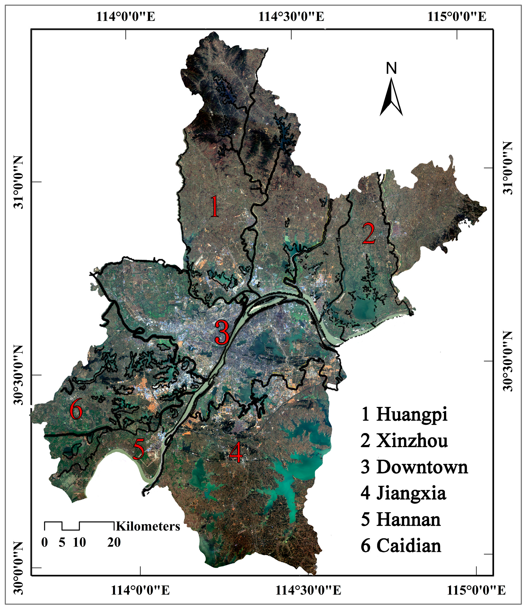
Table 1 shows the Landsat 8 images that were used in this study, downloaded from the Open Spatial Data Sharing system (http://ids.ceode.ac.cn). Then, the quadratic polynomial and nearest neighbor domain interpolation methods were used to perform geo-referencing to UTM (Universal Transverse Mercator, north 49th zone), based on the control points derived from a 1:50,000 topographic map [23], with an error within 0.5 pixels. Following this, a full coverage of Wuhan City was obtained by mosaicking images of the three continuous but different orbital tracks. Finally, the research area was obtained by masking out areas lying outside the administrative vector boundaries of Wuhan (Figure 1). The software used in the preprocessing progress was ENVI 5.0.
2.2. Methodology
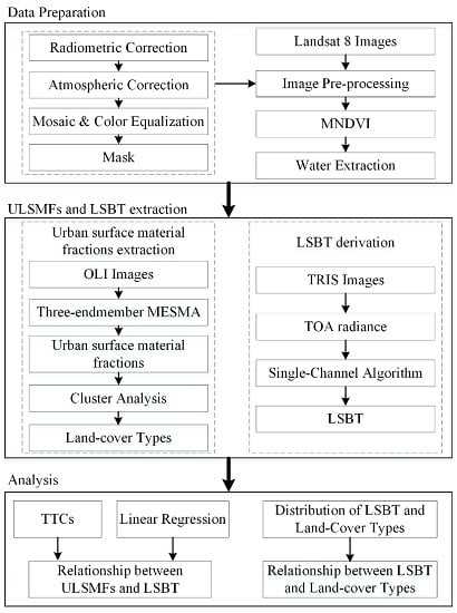
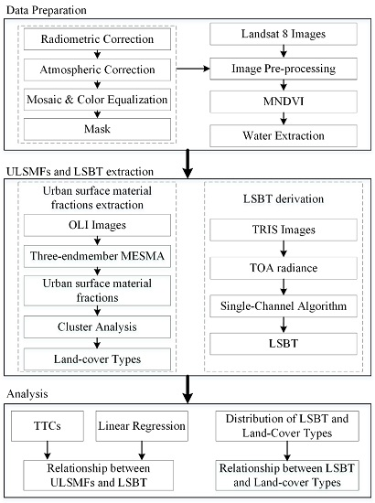
Figure 2 illustrates the overall research framework. A MESMA method was applied to extract the fractions of vegetation, impervious surface, and bare soil within each pixel. The LSBT data were derived from the radiation from the top of the atmosphere, provided by Landsat 8 TRIS images. Then, a clustering analysis and a TTC, as well as multiple linear regression models, were applied to ascertain the relationship between the fraction and the LSBT for every pixel. After having analyzed the contributions of the fractions, we found that the analytical results of both the impervious surface and vegetation were significant, thus indicating a close relationship between the endmember fractions and the aestival LSBT data of Wuhan City.
ENVI 5.0 plug-ins called VIPER (Visualization and Image Processing for Environmental Research) tools were used to extract and optimize the endmember spectrum libraries, as well as three-endmember-MESMA processing. LSBT data were calculated by using ENVI 5.0.
2.2.1. Urban Land Surface Material Fractions on the Basis of MESMA
MESMA is formed by expanding a linear spectral mixture analysis (LSMA) [13,24], which uses only a single, fixed endmember spectrum library to match pixels; however, it is unable to reflect complex spectral diversity. Improving on LSMA, the MESMA method decomposes each pixel with different types of endmember combinations, thus overcoming the inevitable limitations of LSMA [14]. The main improvements of the MESMA method are as follows: (1) for every pixel, MESMA unmixing uses multi-class endmember spectral libraries, which contain a plurality of pure endmember spectra; (2) the MESMA method uses a variety of parameters to optimize the endmember spectrum [25], and this measure makes the spectral libraries more typical; and (3) when unmixing mixed pixels, the MESMA dynamic analysis weights each endmember spectra. The MESMA method can more accurately express endmember diversity and spectrum diversity, reduce the global error, and establish more reasonable models.
For the first step of the MESMA procedure, the optimal spectral libraries were built for classifying our experimental swatch, such as impervious surfaces. Considering the configuration characteristics of urban surface materials [5], and to ensure the diversification of endmember spectra, a visual interpretation was used to process high-resolution images downloaded from Google Earth and selected the regions of interest (the ROIs) that belonged to vegetation, impervious surface, bare soil, crops, and water, all of which contained a large number of endmembers. The EMC function of VIPER Tools was adopted to screen the typical optimal endmember spectra according to the following judgment parameters [14]: (1) Count-based endmember selection (COB). The best endmember spectrum within an interest region would have the highest COB value, thus suggesting that this particular spectrum can simulate a maximum number of spectra in this spectral library [26]; (2) Endmember Average RMSE (EAR) [27], which is expressed by Equation (1). When using a spectrum to simulate each spectrum in an ROI, the average simulation qualities were evaluated by calculating the mean EAR to simplify the unmixing procedure. The best simulation quality for an ROI would have the lowest EAR; (3) Minimum Average Spectral Angle (MASA, Equation (5)) [28]: MASA parameters were used to compare the differences between different ROIs, and thus the most typical spectra case for every land-cover type was obtained.
In Equation (1), and express the “Endmember Spectra” class and “Modeled Spectra” class, respectively; n shows the number of in the class, and n − 1 simulation models are obtained by using all of the . In addition, belongs to the class.
In calculating the spectral angle θ between two spectral vectors (Equation (2)), and , respectively, express the endmember spectrum vectors and the modeled spectrum (Equation (3)); M represents the number of bands; is the residual error; and and express the reflectivity of band and the modeling spectra, respectively (Equation (4)). When we assume that there are N bands, is the band λ reflectivity of the endmember i. In Equation (5), n shows the number of in the B class, which represents the modeled spectra class, and we can obtain n − 1 simulation models by using all of the .
After the filtering processing, the original endmember spectral libraries that contained many endmembers (non-pure endmember) were streamlined into optimal endmember spectral libraries. Then, the three spectral libraries were imported into VIPER tools and the MESMA procedure was executed [29]. As a result, the preprocessed satellite images were decomposed into three fraction images: green vegetation, impervious surfaces, and bare soil [14].
2.2.2. Land Surface Brightness Temperature Derivation
The Landsat 8 TIRS (thermal infrared sensor) collects radiation data at the top of the atmosphere. According to Planck’s law, assuming that the content of vapor is relatively small and constant in the atmosphere (the radiation change affected by atmospheric conditions can only be ignored when there exists a homogeneous atmospheric environment), the at-satellite brightness temperature (in Kelvin) reflects the surficial temperature distribution condition on land [6,30]. Some researchers have proved that the at-satellite brightness temperature can be used to approximate the land surface brightness temperature (LSBT) instead [31,32,33], and some important parameters in [34] cannot easily be obtained in this research, so the at-satellite brightness temperature was used as the LSBT in our research.
The double-near-infrared bands (Bands 10–11) of Landsat 8 provide raw radiation luminance [35]. The after-corrected metadata listed the correction parameters [36], the units of gains and offsets are w/(m2*sr*μm), K1 and K2’s are Kelvin (Equation (6)), and the radiation values were obtained as (w/(m2*sr*μm)) data. Finally, these values were converted into the brightness temperature (T) (in Kelvin, Equation (7)). In this study, Band 10 was used to calculate the brightness temperature.
2.2.3. Ternary Triangular Chart
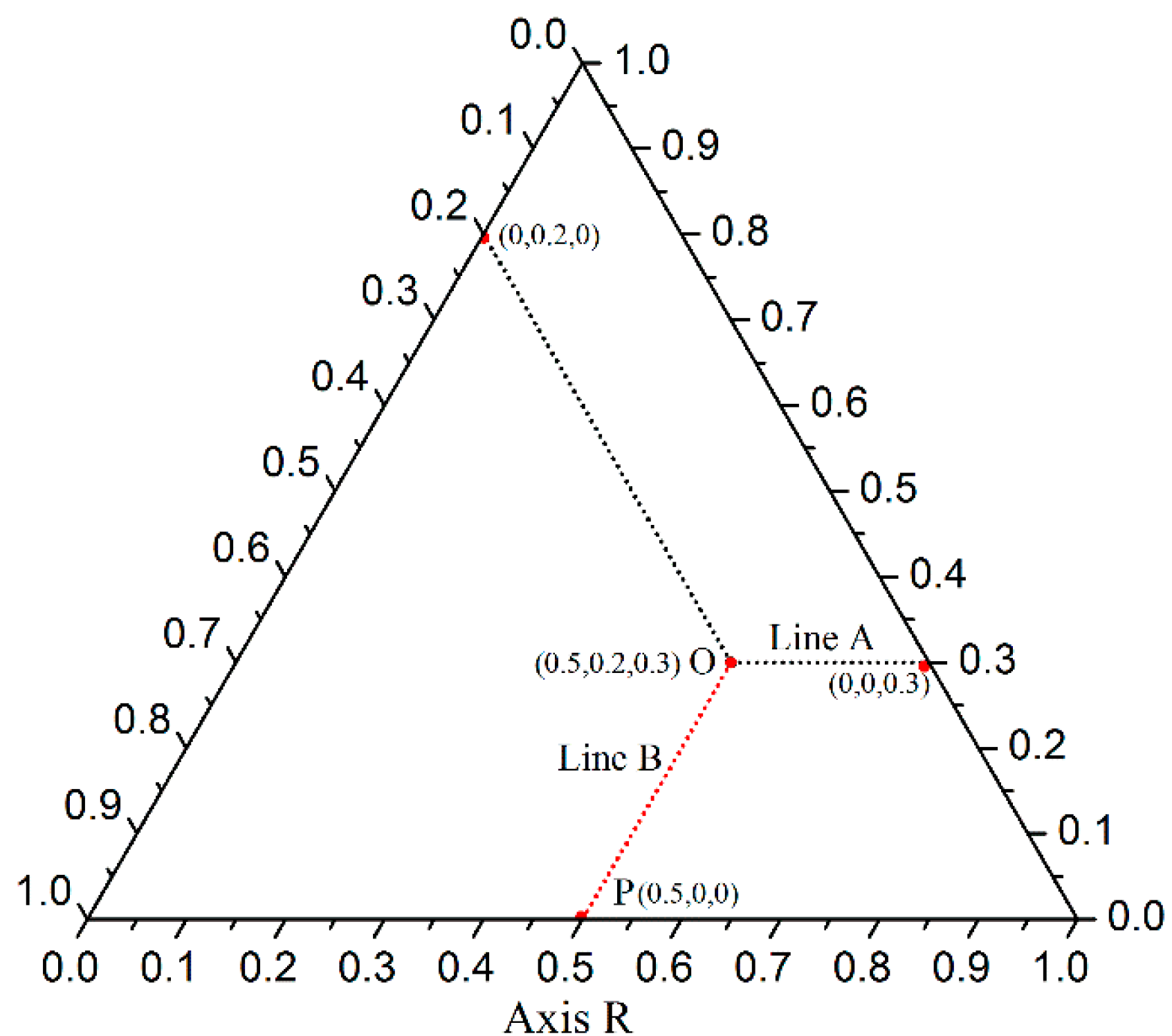
The Ternary triangular chart is drawn on the mineral classification method, which is used to determine the composition, generating the TTC to locate every pixel on the basis of the fractions (Figure 3).
An equilateral triangle projection was generated for the endmember fraction data, which are expressed as the coverage proportion of land-cover types in a pixel: for any point O on the chart, we assumed that an auxiliary line A over point O is parallel to the axis R. Then, point O was adopted as the starting point and we assumed another auxiliary line B over O that was parallel to another axis and crossed axis R at point P. The value of intersection P was the fraction on axis R. The other two intersections, formed by line A that crossed the other two axes, were both fractions. In this way, the three endmember spectra class fractions of point O were obtained. Thus, we located a point on the basis of the fractions for each sample point (but not the geographic coordinates), so any point on the charts represented a different land surface condition. In other words, the same exception of sampling points appeared when and only when there existed two pixels with an identical surface material.
3. Results
3.1. Distribution of Endmember Fractions
Since the study area comprised mainly urban regions, the vegetation-impervious surface-soil (V-I-S) model was selected for unmixing processing [37]. Because water has a single spectral characteristic and it has a high impact on LSBT, it was primarily extracted by using the Modified Normalized Difference Water Index (MNDWI) [38,39] and decomposed water regions (12.62% of the total study area in Figure 4). Then, the spectral libraries of vegetation, impervious surface, and bare soil were substituted, respectively, into the MESMA module, and a total of 48 (eight vegetation × three impervious surface × two soil) linear spectral mixture models were obtained. Each endmember fraction is shown in Figure 5a–c, in which a deeper grey color represents a larger fraction. The subtle fraction data (in pixel-level) met the demand for the precision of subsequent experiments. Figure 5d is the error image of MESMA. A total of 86.93% of the impute images were classified.
Figure 6 shows the RMSE statistical result by pixels. It can be seen from Figure 6 that the mean RMSE of the whole study area is 0.09, with a standard deviation of 0.11. The blue curve (Percent) is the RMSE proportion for the segmented sampling of the statistical results. The peak value of the blue curve is 13.83%, concentrated in the range of 0.0–0.1, which then sharply reduced to 0.06%. The red curve is the segmented cumulative ratio of RMSE. We can see that more than 80.57% of the pixels have an RMSE value of less than 0.1.
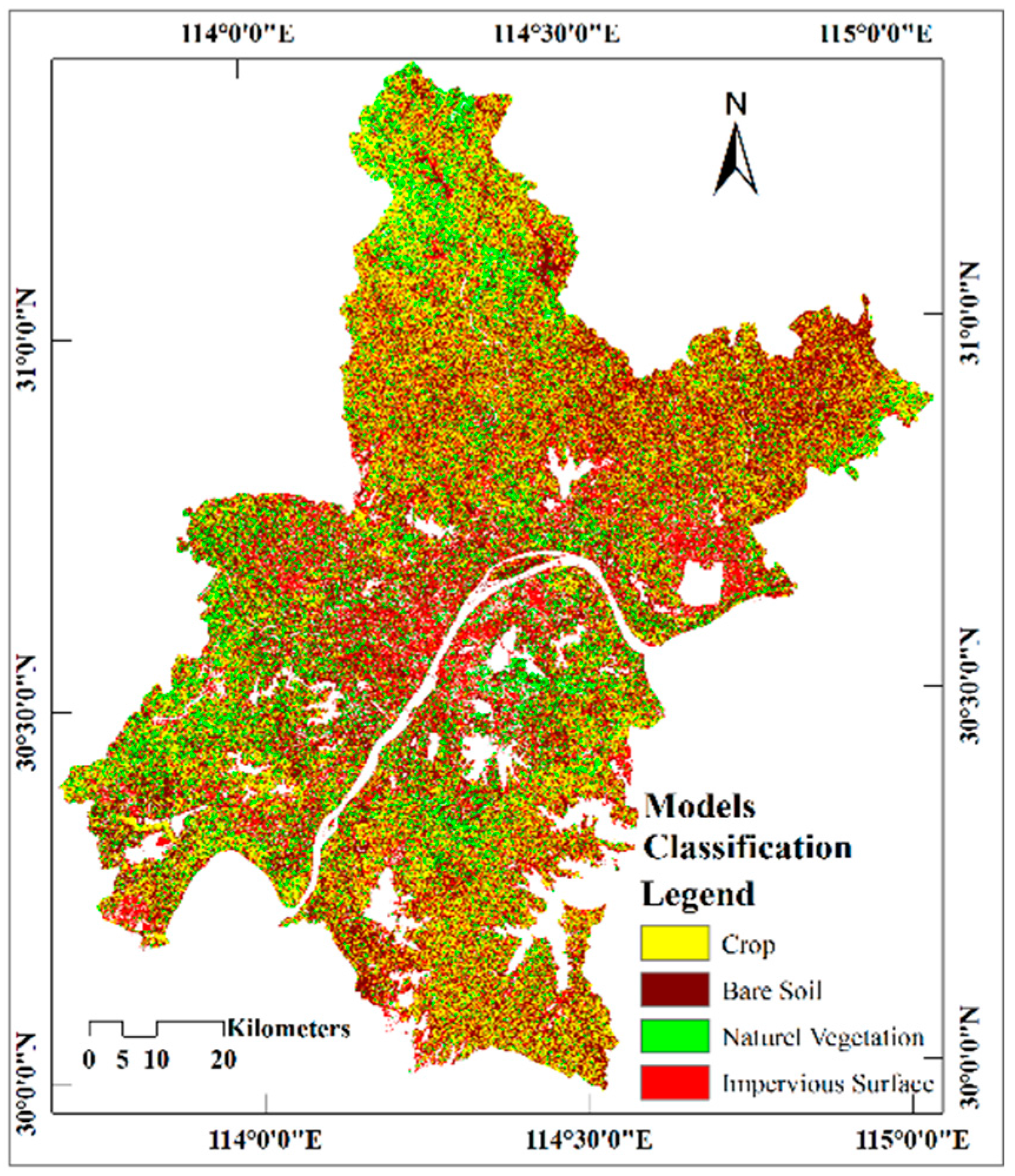
Figure 7 shows the results of the cluster analysis. The properties of the endmember groups were artificially evaluated by referring to the high-resolution images and density segmentation processing. The figure shows the natural vegetation in green (15.54%), the crops in yellow (25.55%), the impervious surfaces in red (17.69%), and the bare soil in sienna (28.18%). A cluster analysis is an unsupervised classification method that only classifies the groups on the basis of the similarities among data, so that the cluster analysis procedures are irrelevant to the threshold of the fractions [19,40,41,42]. Because it has been previously assumed that there exist five categories of typical land uses in the study area (impervious surface, bare soil, natural vegetation, crop, and water) but water regions extracted by MNDWI do not participate in the cluster analysis, four pixel-groups of undefined properties were obtained.
Figure 7 shows the following: (1) The pixels belonging to the impervious surface group are concentrated in urban centers, whereas the sporadic suburban areas have high-density building proportions; (2) The bare soil pixels have a spotty distribution, surrounding the urban center (impervious surfaces). Exposed topsoil is due to planned construction, as well as the re-construction caused by the city’s expansion; in addition, the higher soil fraction surrounding the water regions; (3) The coverage of crop regions is vast; however, the vegetation fraction (containing the natural vegetation and the crops) near the urban center is very low; in contrast, it becomes relatively higher near Jiuzhen Mountain in Caidian District, the northern hilly terrain in Huangpi District, and Xinzhou District, as well as other areas.
3.2. Aestival LSBT Distribution
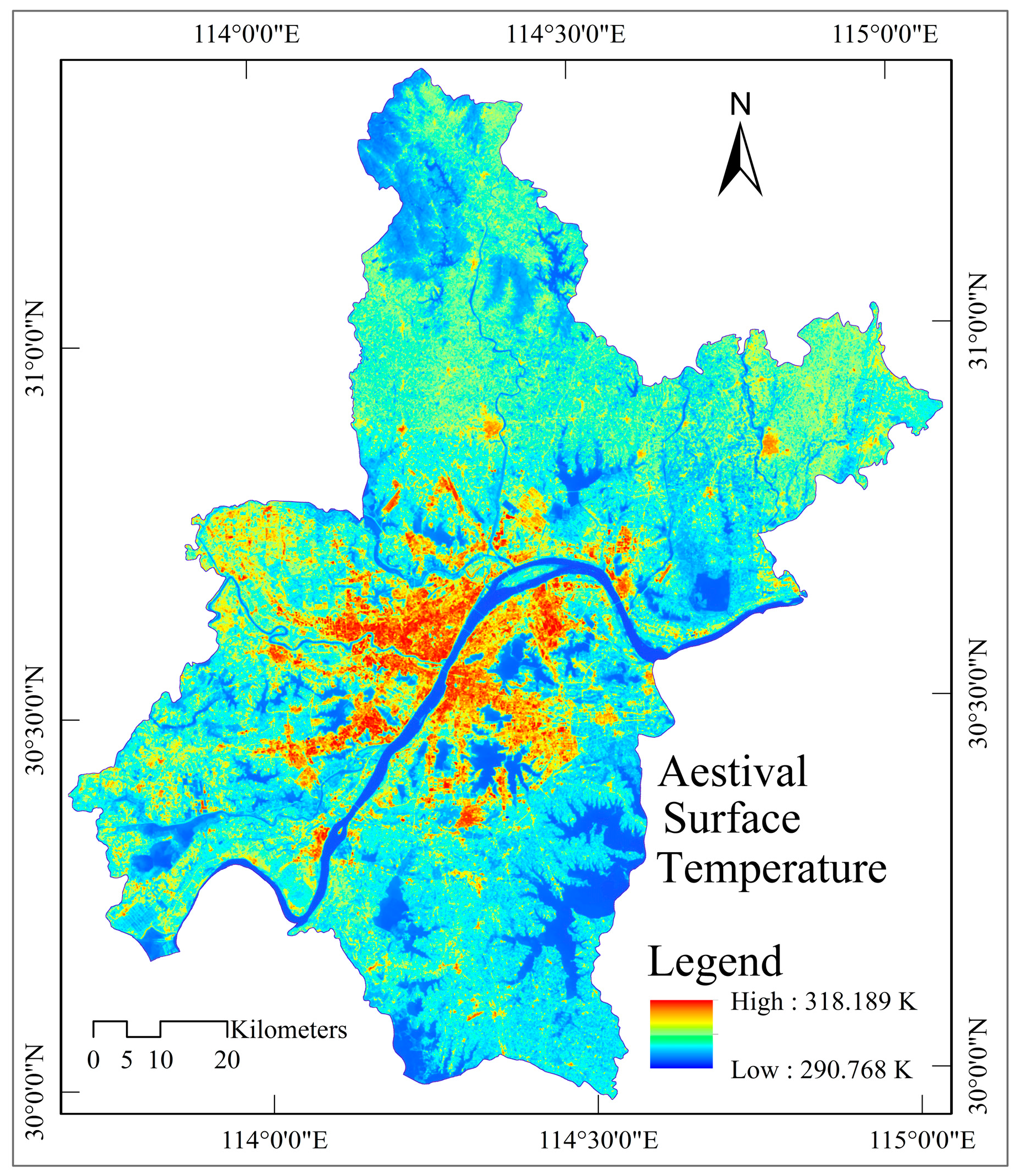
For climatic reasons, the satellite images taken in the early summer were selected (late June); therefore, the average temperature obtained is relatively lower than that in other LSBT inversion studies [22]. Figure 8 shows that a significant heat island phenomenon occurred in Wuhan, in which the highest temperature was concentrated in the urban centers and the local-secondary business districts, whereas water regions and the suburbs were covered with a relatively lower LSBT. In addition, the overall area exhibited large differences in temperature (the standard deviation reached 2.81 Kelvin).
The Center Cities have a large amount of impervious surface, most of which comprise heavily populated old cities, heavy industrial zones, highly commercialized sub-centers, clusters of processing and manufacturing industries, asphalt roads, and other areas where water is scarce, but artificial building materials (such as asphalt, concrete, metal, etc.) are abundant and vegetation coverage is low [31]. The above characteristics provide impervious surfaces with a high heat radiation ability; therefore, these surfaces are the major contributors to the urban heat effect. In addition, the surrounding development zones that have a large amount of bare soil and few impervious surfaces, with almost no vegetation, showed a high LSBT. Nevertheless, the bare soil provided the second-highest contribution rate for the thermal effect because its human activities are relatively weak. Finally, the natural vegetation’s LSBT was approximately 1–2 K lower than that of the crops, which was even lower than the high LSBT of the two types noted above. The photosynthesis and the evapotranspiration in plants increase, and the moisture proportion is higher, when the natural vegetation fractions become higher [31]. In addition, the large crowns of natural vegetation are wider than the canopy of crops and are able to prevent solar radiation from reaching the land [43,44,45,46,47]. Under normal circumstances, the LSBT of rivers is slightly lower than that of lakes [31]; however, there are some exceptions, such as when the rivers flow through city centers and the water near river banks and lake edges, where the LSBT will be slightly increased.
3.3. Relationship between ULSMFs and LSBT
In this paper, a statistical analysis of the aestival LSBT and its averages was gathered, and the data were processed through a cluster analysis. From Figure 8, an obviously strong phenomenon of an urban heat island was observed in the summer, and the overall temperature difference in our study area reached up to 30 K.
To conduct follow-up research, approximately 130,000 random sample points were first collected through ArcGIS 10.1, after having overlapped the fraction layers with the data layers of aestival LSBT. Then, the data from the sampled points were processed by using OriginPro 8.6 software to generate the TTC (Figure 9a). Finally, multivariate linear regression equations were used to fit the relationship between the fractions and the LSBT data.
Figure 9b is the hypsometric ternary triangle chart for the aestival LSBT, which shows that the intensity of red areas increased as the impervious surface fractions increased and the vegetation decreased, whereas the LSBT only changed very slightly with fluctuations in the bare soil fraction. When the vegetation fraction was greater than 0.5, the capability of the vegetation to regulate temperature was strong, whereas when the impervious surface fraction reached 0.5, the densities of the red high temperature zones surged. Therefore, the fractions of impervious surface and vegetation have a high impact on the aestival LSBT.
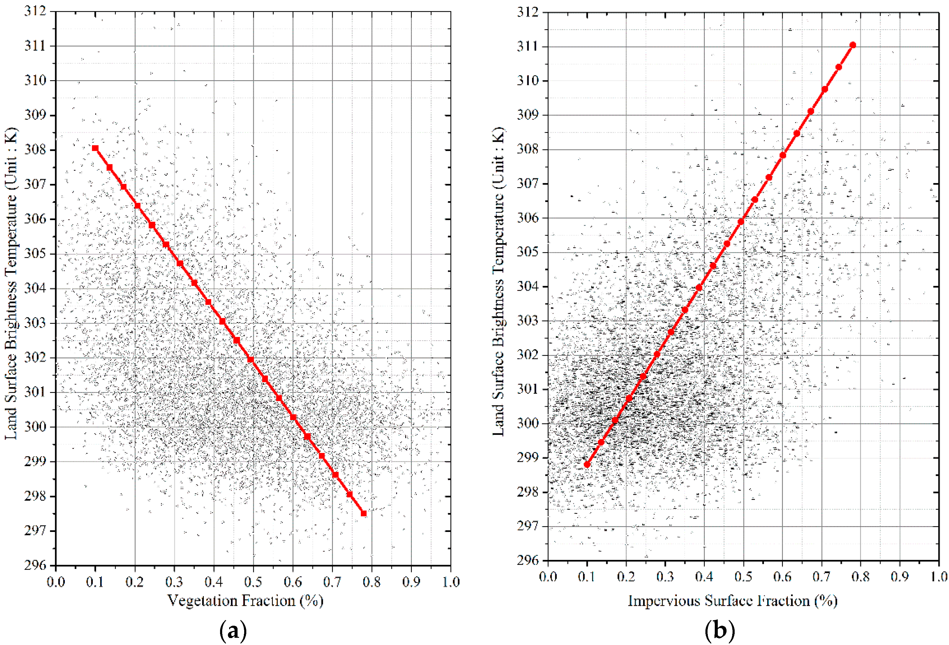
OriginPro 8.6 was used to generate scatter plots (Figure 10a,b), which showed a relatively clear linear relationship between the aestival LSBT and the fraction of vegetation (or the impervious surface fraction). Then, SPSS Statistics 19 was used to fit the multivariate linear regression equations to determine the mathematical relationship between the aestival LSBT data and the endmember fractions [48,49,50]. The fitted results (Equations (8)–(10)) indicated a significant linear relationship, of which the probability values (respectively, in the F test, for the regression equation’s significance, as well as the T test, for the regression coefficients’ significance) were less than the 0.05 significance level (Table 2).
where , , and stand for the of vegetation, impervious surface, and all three endmembers, respectively. , , and represent the fraction of vegetation, impervious surface, and bare soil, respectively.
From Figure 10a, it can be seen that the vegetation had a significant regulatory effect on temperature (high temperatures can be reduced when there is a large vegetation fraction). When its fraction came close to or exceeded 0.6, the LSBT values tended to be more stable at approximately 298–300 K (approximately 25–27 °C). The Adj. R2 of the regression Equation (8) was 0.88, thus indicating that the vegetation fraction (as the independent variable) can explain 88% of the change in the summer LSBT (as the dependent variable).
The high impervious surface endmember fraction was significantly positively correlated with the high aestival LSBT, thus explaining 90.2% of the change in the aestival LSBT and indicating a significant linear relationship (Equation (9), Table 2). The higher impervious surface fraction had poor water retention, as well as almost no vegetation coverage.
In a comprehensive analysis, it can be found that when the endmember fractions of the above three categories were used as different independent variables, the fitted multivariate regression equation obtained (Equation (10)) had an Adj. R2 of 0.986, thus indicating that this combination of endmember spectra explains 98.6% of the changes in the aestival LSBT.
4. Discussion
Many researches have been concentrated on the relationship between land-use/cover and surface temperature [1,51,52,53,54], but they have ignored the mixed pixel in the image. In our research, we focus on the relationship between ULSMFs fractions and LSBT, which means that we classified one pixel into three components and analysed the relationship between the fractions and LSBT, achieving an accuracy of 98.6% in multivariate regression analysis.
In an urban area, manmade materials, especially the impervious surfaces, have a significant positive effect on LSBT (Figure 10b). The correlation analysis results (Table 2) also show the same results. This finding is consistent with some other studies [1,51,54].
Vegetation which can lower the LSBT by releasing more latent heat flux through the evapotranspiration progress displays an effective mitigation strategy to reduce the LSBT [52,53]. Our correlation analysis shows that the vegetation fraction has a negative relationship with the LSBT, which indicates that the increase of the vegetation fraction can lower the LSBT in the urban area.
Bare soil is a transitional phase, which is intermediate in the transition from a vegetation surface (natural environment) to an impervious surface (artificial environment). Owing to the temperature regulation of vegetation and the warming effects of impervious surfaces, a separate discussion of the bare soil fraction data is necessary: (1) In the low-temperature region in the summer (≤302 K), the vegetation fraction was relatively high (>0.4), whereas the impervious surface fraction was low; (2) In the high-temperature region (≥302 K), the aestival LSBT increased when the impervious surface fraction increased, and both the fraction of vegetation and soil were significantly reduced.
Although we can obtain a satisfactory accuracy in the correlation analysis between the endmember fraction and LSBT, some uncertainties still remain. First of all, the selection of pure endmember spectra in the MESMA process can introduce uncertainties. Although the high spatial resolution images can be used, errors are inevitable. Second, the error analysis of the MESMA results is still a problem in the validation process, which will form the research focus in the future.
5. Conclusions
In this paper, MESMA was applied to extract the V-I-S fractions and the brightness temperatures were derived from the radiation exhibited in the upper atmosphere. Then, the TTC method, as well as linear-regression analysis, was used to explore the relationship between the composition of the ULSMFs and the performance of the surficial thermal environment in the summer. The conclusions are as follows: MESMA is able to interpret the urban surficial material constitution, and the fractions cluster result was consistent with Wuhan City planning in the same period.
From a qualitative point of view, Wuhan experiences a considerable urban heat island phenomenon in the summer, and the surface material types and LSBT are significantly correlated, especially impervious surfaces and the heat island.
The quantitative multivariate regression analysis results showed that the different compositions of surface materials used to fit multiple linear regression models were all able to effectively explain the aestival LSBT performance in Wuhan; in other words, the types of surface material and the changes in surficial compositions have a close relationship with LSBT.
The hypsometric TTCs can visualize the relationship between endmember fractions and the LSBT, thus enhancing the practical value of the application of MESMA.
In the summer, the LSBT is mainly influenced by the vegetation and impervious surface endmember fractions. The results revealed the importance of plants in regulating the temperature in the city. The complicated surface composition influences the thermal environment of urban regions, thus indicating that sustainable development should take these factors into account.
Acknowledgments
This work was supported in part by the National Natural Science Foundation of China (61601418); and in part by the National High Technology Research and Development Program of China (2012AA121303). The authors would like to thank the handling editor and anonymous reviewers for their valuable comments and suggestions, which significantly improved the quality of this paper.
Author Contributions
Tao Chen and Xujia Zhang implemented the urban land surface material fractions extraction and brightness temperature derivation methods, and conducted the experiments; Xujia Zhang finished the first draft; Tao Chen and Ruiqing Niu supervised the research and contributed to the editing and review of the manuscript.
Conflicts of Interest
The authors declare no conflict of interest.
Abbreviations
The following abbreviations are used in this manuscript:
| CCCD | Continuous Classification and Change Detection |
| LSBT | Land Surface Brightness Temperature |
| LSMA | Linear Spectral Mixture Analysis |
| MESMA | Multiple Endmember Spectral Mixture Analysis |
| MNDWI | Modified Normalized Difference Water Index |
| NDVI | Normalized Difference Vegetation Index |
| OBIA | Object-based Image Analysis |
| TTC | Ternary Triangular Chart |
| ULSMFs | Urban Land Surface Material Fractions |
| UTM | Universal Transverse Mercator |
| VIPER | Visualization and Image Processing for Environmental Research |
References
- Chen, X.L.; Zhao, H.M.; Li, P.X.; Yin, Z.Y. Remote sensing image-based analysis of the relationship between urban hear island and land use/cover changes. Remote Sens. Environ. 2006, 104, 133–146. [Google Scholar] [CrossRef]
- Xia, J.; Du, P.; Zhang, H.; Liu, P. The quantitative relationship between land surface temperature and land cover types based on remotely sensed data. Remote Sens. Technol. Appl. 2010, 25, 15–23, (In Chinese with English Abstract). [Google Scholar]
- Tian, P.; Tian, G.; Wang, F.; Wang, Y.F. Urban heat island effect and vegetation cover index relation using Landsat TM image. Bull. Sci. Technol. 2006, 22, 708–713, (In Chinese with English Abstract). [Google Scholar]
- Zhou, H.M.; Zhou, C.H.; Ge, W.Q.; Ding, J.C. The surveying on thermal distribution in urban based on GIS and remote sensing. Acta Geogr. Sin. 2001, 56, 189–197, (In Chinese with English Abstract). [Google Scholar]
- Chen, Y.; Wang, J.; Li, X. A study on urban thermal field in summer based on satellite remote sensing. Remote Sens. Land Resour. 2002, 14, 55–59, (In Chinese with English Abstract). [Google Scholar]
- Li, X.X.; Myint, S.W.; Zhang, Y.; Galletti, C.; Zhang, X.; Turner, B.L. Object-based land-cover classification for metropolitan Phoenix, Arizona, using aerial photography. Int. J. Appl. Earth Obs. Geoinf. 2014, 33, 321–330. [Google Scholar] [CrossRef]
- Li, X.X.; Li, W.W.; Middel, A.; Harlan, S.L.; Brazel, A.J.; Turner, B.L. Remote sensing of the surface urban heat island and land architecture in Phoenix, Arizona: Combined effects of land composition and configuration and cadastral-demographic-economic factors. Remote Sens. Environ. 2016, 174, 233–243. [Google Scholar] [CrossRef]
- Zhu, Z.; Woodcock, C.E. Continuous change detection and classification of land cover using all available Landsat data. Remote Sens. Environ. 2014, 144, 152–171. [Google Scholar] [CrossRef]
- Fu, P.; Weng, Q. A time series analysis of urbanization induced land use and land cover change and its impact on land surface temperature with Landsat imagery. Remote Sens. Environ. 2016, 175, 205–214. [Google Scholar] [CrossRef]
- Michishita, R.; Jiang, Z.B.; Xu, B. Monitoring two decades of urbanization in the Poyang Lake area, China through spectral unmixing. Remote Sens. Environ. 2012, 117, 3–18. [Google Scholar] [CrossRef]
- Lu, D.S.; Moran, E.; Batistelia, M. Linear mixture model applied to Amazonian vegetation classification. Remote Sens. Environ. 2003, 87, 456–469. [Google Scholar] [CrossRef]
- Phinn, S.; Stanford, M.; Scarth, P. Monitoring the composition of urban environments based on the vegetation-impervious surface-soil (VIS) model by subpixel analysis techniques. Remote Sens. Environ. 2002, 23, 4131–4153. [Google Scholar] [CrossRef]
- Roberts, D.A.; Gardner, M.; Church, R.; Ustin, S.; Scheer, G.; Green, R.O. Mapping Chaparral in the Santa Monica Mountains Using Multiple Endmember Spectral Mixture Models. Remote Sens. Environ. 1998, 65, 267–279. [Google Scholar] [CrossRef]
- Quintano, C.; Fernández-Manso, A.; Roberts, D.A. Multiple Endmember Spectral Mixture Analysis (MESMA) to map burn severity levels from Landsat images in Mediterranean countries. Remote Sens. Environ. 2013, 136, 76–88. [Google Scholar] [CrossRef]
- Quintano, C.; Fernandez-Manso, A.; Roberts, D.A. Burn severity mapping from Landsat MESMA fraction images and Land Surface Temperature. Remote Sens. Environ. 2017, 190, 83–95. [Google Scholar] [CrossRef]
- Zhang, Z.M.; He, G.J.; Dai, Q.; Jiang, H. Leaf Area Index Estimation Using MESMA Based on EO-1 Hyperion Satellite Imagery. Int. J. Inf. Electron. Eng. 2014, 4, 11–15. [Google Scholar] [CrossRef]
- Zhang, M.; Huang, S.; Feng, W. Further calculating plots in a triangle for the classification of sandstones. J. Chengdu Univ. Technol. Sci. Technol. Ed. 2005, 32, 421–429. [Google Scholar]
- Arnone, R.; Loisel, H.; Carder, K.; Boss, E.; Maritorena, S.; Lee, Z. Remote Sensing of Inherent Optical Properties: Fundamentals, Tests of Algorithms, and Applications; IOCCG Report 2006; International Ocean-Colour Coordinating Group: Hanover, NH, USA, 2006; Volume 5, pp. 95–100. [Google Scholar]
- Uitz, J.; Stramski, D.; Reynolds, R.A.; Dubranna, J. Assessing phytoplankton community composition from hyperspectral measurements of phytoplankton absorption coefficient and remote-sensing reflectance in open-ocean environments. Remote Sens. Environ. 2015, 171, 58–74. [Google Scholar] [CrossRef]
- Xin, X.; Zhang, P. Vulnerability classification in man-land territorial system of mining cities based on triangle methodology. J. China Coal Soc. 2009, 34, 284–288, (In Chinese with English Abstract). [Google Scholar]
- Xu, F.; Zhao, S.; Zhang, Y.; Hao, J.; Zhan, W. A methodology for evaluating quantitatively the sustainability status and trends of economic development. Acta Sci. Circumst. 2005, 25, 711–720, (In Chinese with English Abstract). [Google Scholar]
- Wu, H.; Ye, L.P.; Shi, W.Z.; Clarke, K.C. Assessing the effects of land use spatial structure on urban heat islands using HJ-1B remote sensing imagery in Wuhan, China. Int. J. Appl. Earth Obs. Geoinf. 2014, 32, 67–78. [Google Scholar] [CrossRef]
- Makarau, A.; Richter, R.; Schläpfer, D.; Reinartz, P. Combined haze and cirrus removal for multispectral imagery. IEEE Geosci. Remote Sens. Lett. 2016, 13, 379–383. [Google Scholar] [CrossRef]
- Roberts, D.A.; Smith, M.O.; Adams, J.B. Green vegetation, nonphotosynthetic vegetation, and soils in AVIRIS data. Remote Sens. Environ. 1993, 44, 255–269. [Google Scholar] [CrossRef]
- Fan, F.; Deng, Y. Enhancing endmember selection in multiple endmember spectral mixture analysis (MESMA) for urban impervious surface area mapping using spectral angle and spectral distance parameters. Int. J. Appl. Earth Obs. Geoinf. 2014, 33, 290–301. [Google Scholar] [CrossRef]
- Roberts, D.A.; Dennison, P.E.; Gardner, M.E.; Hetzel, Y. Evaluation of the potential of Hyperion for fire danger assessment by comparison to the Airborne Visible/Infrared Imaging Spectrometer. IEEE Trans. Geosci. Remote Sens. 2003, 41, 1297–1310. [Google Scholar] [CrossRef]
- Dennison, P.E.; Roberts, D.A. Endmember selection for multiple endmember spectral mixture analysis using endmember average RMSE. Remote Sens. Environ. 2003, 87, 123–135. [Google Scholar] [CrossRef]
- Dennison, P.E.; Halligan, K.Q.; Roberts, D.A. A comparison of error metrics and constraints for multiple endmember spectral mixture analysis and spectral angle mapper. Remote Sens. Environ. 2004, 93, 359–367. [Google Scholar] [CrossRef]
- Vassilopoulou, V.; Katsanevakis, S.; Panayotidis, P.; Anagnostou, C.; Damalas, D.; Dogrammatzi, A.; Drakopoulou, V.; Giakoumi, S.; Haralabous, J.; Issaris, Y.; et al. Application of the MESMA Framework. Case Study: Inner Ionian Archipelago & Adjacent Gulfs. 2012. Available online: http://www.mesma.org/FILE_DIR/06-10-2013_13-42-31_16_3_MESMA-FW-Case-Study-Greece.pdf (accessed on 25 May 2017).
- Ozelkan, E.; Bagis, S.; Ozelkan, E.C.; Ustundag, B.B.; Ormeci, C. Land Surface Temperature Retrieval for Climate Analysis and Association with Climate Data. Eur. J. Remote Sens. 2014, 47, 655–669. [Google Scholar] [CrossRef]
- Feizizadeh, B.; Blaschke, T. Examining urban heat island relations to land use and air pollution: Multiple endmember spectral mixture analysis for thermal remote sensing. IEEE J. Sel. Top. Appl. Earth Obs. Remote Sens. 2013, 6, 1749–1756. [Google Scholar] [CrossRef]
- Dash, P.; Göttsche, F.M.; Olesen, F.S.; Fischer, H. Land surface temperature and emissivity estimation from passive sensor data: Theory and practice-current trends. Int. J. Remote Sens. 2002, 23, 2563–2594. [Google Scholar] [CrossRef]
- Pareeth, S.; Salmaso, N.; Adrian, R.; Neteler, M. Homogenised daily lake surface water temperature data generated from multiple satellite sensors: A long-term case study of a large sub-Alpine lake. Sci. Rep. 2016, 6, 31251. [Google Scholar] [CrossRef] [PubMed]
- Yu, X.; Guo, X.; Wu, Z. Land surface temperature retrieval form Landsat 8 TIRS—Comparison between radiative transfer equation based method, split window algorithm and single channel method. Remote Sens. 2014, 6, 9829–9852. [Google Scholar] [CrossRef]
- Coll, C.; Galve, J.M.; Sanchez, J.M.; Caselles, V. Validation of Landsat-7/ETM+ Thermal-Band Calibration and Atmospheric Correction with Ground-Based Measurements. IEEE Trans. Geosci. Remote Sens. 2010, 48, 547–555. [Google Scholar] [CrossRef]
- Chander, G.; Markham, B.L.; Helder, D.L. Summary of current radiometric calibration coefficients for Landsat MSS, TM, ETM+, and EO-1 ALI sensors. Remote Sens. Environ. 2009, 113, 893–903. [Google Scholar] [CrossRef]
- Ridd, M.K. Exploring a VIS (vegetation-impervious surface-soil) model for urban ecosystem analysis through remote sensing: Comparative anatomy for cities. Int. J. Remote Sens. 1995, 16, 2165–2185. [Google Scholar] [CrossRef]
- Xu, H. Modification of normalized difference water index (NDWI) to enhance open water features in remotely sensed imagery. Int. J. Remote Sens. 2006, 27, 3025–3033. [Google Scholar] [CrossRef]
- Sheng, Y.W.; Song, C.Q.; Wang, J.D.; Lyons, E.A.; Knox, B.R.; Cox, J.S.; Gao, F. Representative lake water extent mapping at continental scales using multi-temporal Landsat-8 imagery. Remote Sens. Environ. 2016, 185, 129–141. [Google Scholar] [CrossRef]
- Celebi, M.E.; Kingravi, H.A.; Vela, P.A. A comparative study of efficient initialization methods for the k-means clustering algorithm. Expert Syst. Appl. 2013, 40, 200–210. [Google Scholar] [CrossRef]
- Field, A. Discovering Statistics Using IBM SPSS Statistics, 4th ed.; Sage Publications Ltd.: Los Angeles, CA, USA, 2013. [Google Scholar]
- Gouveia, C.M.; Trigo, R.M.; Beguería, S.; Vicente-Serrano, S.M. Drought impacts on vegetation activity in the Mediterranean region: An assessment using remote sensing data and multi-scale drought indicators. Glob. Planet. Chang. 2016. [Google Scholar] [CrossRef]
- Zhang, Y.; Li, Z. Remote sensing of atmospheric fine particulate matter (PM2.5) mass concentration near the ground from satellite observation. Remote Sens. Environ. 2015, 160, 252–262. [Google Scholar] [CrossRef]
- Asmala, A.; Shaun, Q. Haze modelling and simulation in remote sensing satellite data. Appl. Math. Sci. 2014, 8, 7909–7921. [Google Scholar]
- Zhang, Z.; Zhang, X.; Gong, D.; Kim, S.J.; Mao, R.; Zhao, X. Possible influence of atmospheric circulations on winter haze pollution in the Beijing–Tianjin–Hebei region, northern China. Atmos. Chem. Phys. 2016, 16, 561–571. [Google Scholar] [CrossRef]
- Wang, H.; Chen, H. Understanding the recent trend of haze pollution in eastern China: Roles of climate change. Atmos. Chem. Phys. 2016, 16, 4205–4211. [Google Scholar] [CrossRef]
- Tian, M.; Wang, H.B.; Chen, Y.; Yang, F.M.; Zhang, X.H.; Zou, Q.; Zhang, R.Q.; Ma, Y.L.; He, K.B. Characteristics of aerosol pollution during heavy haze events in Suzhou, China. Atmos. Chem. Phys. 2015, 15, 33407–33443. [Google Scholar] [CrossRef]
- Johnson, R.A.; Wichern, D.W. Applied Multivariate Statistical Analysis, 6th ed.; Prentice Hall: Upper Saddle River, NJ, USA, 2002. [Google Scholar]
- Souza, J.B.D.; Santos, J.M. Principal Components and generalized linear modeling inthe correlation between hospital admissions and air pollution. Rev. Saúde Pública 2014, 48, 451–458. [Google Scholar] [CrossRef] [PubMed]
- Recio-Vazquez, L.; Almendros, G.; Knicker, H.; Carral, P.; Álvarez, A.M. Multivariate statistical assessment of functional relationships between soil physical descriptors and structural features of soil organic matter in Mediterranean ecosystems. Geoderma 2014, 230–231, 95–107. [Google Scholar] [CrossRef]
- Wang, C.; Myint, S.W.; Wang, Z.; Song, J. Spatio-temporal modeling of the urban heat island in the Phoenix metropolitan area: Land use change implications. Remote Sens. 2016, 8, 185. [Google Scholar] [CrossRef]
- Myint, S.W.; Wentz, E.A.; Brazel, A.J.; Quattrochi, D.A. The impact of distinct anthropogenic and vegetation features on urban warming. Landsc. Ecol. 2013, 28, 959–978. [Google Scholar] [CrossRef]
- Zheng, B.; Myint, S.W.; Fan, C. Spatial configuration of anthropogenic land cover impacts on urban warming. Landsc. Urban Plan. 2014, 130, 104–111. [Google Scholar] [CrossRef]
- Weng, Q. A remote sensing-GIS evaluation of urban expansion and its impact on surface temperature in the Zhujiang Delta, China. Int. J. Remote Sens. 2001, 22, 1999–2014. [Google Scholar] [CrossRef]
Figure 1.
Location of the study area (R: Band4, G: Band3, B: Band2).

Figure 2.
Flow chart of the proposed methods in this study.
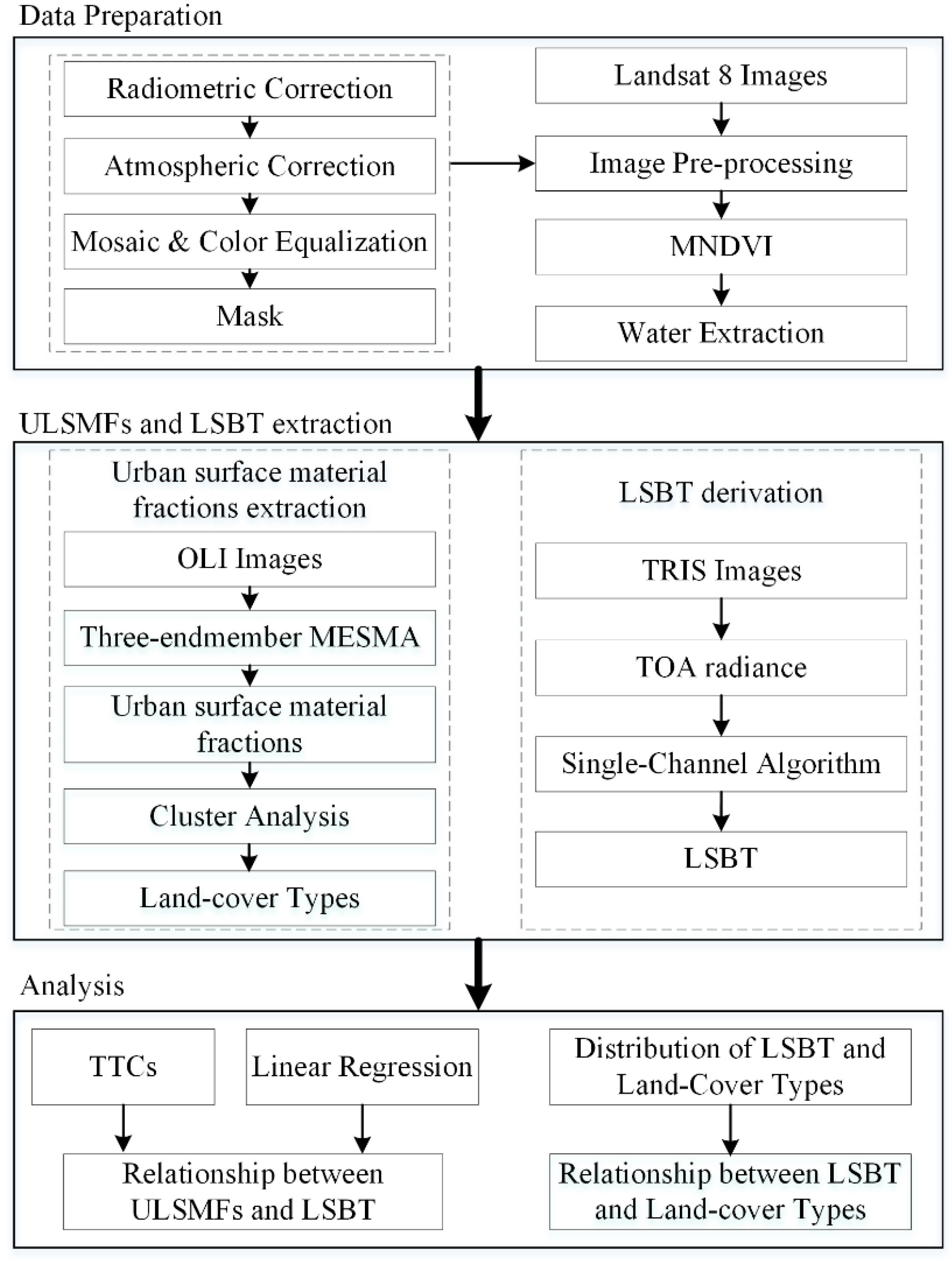
Figure 3.
Schematic of the ternary triangular chart.

Figure 4.
The extraction result of water.
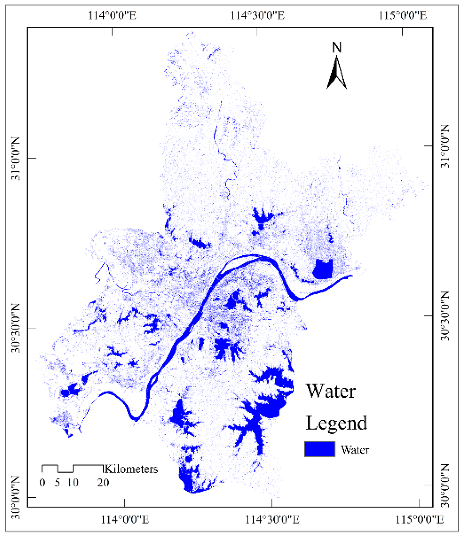
Figure 5.
The result of three-endmember spectral mixture analysis (3em-MESMA). (a) Fraction of vegetation; (b) fraction of impervious surface; (c) fraction of soil; (d) error image.
Figure 5.
The result of three-endmember spectral mixture analysis (3em-MESMA). (a) Fraction of vegetation; (b) fraction of impervious surface; (c) fraction of soil; (d) error image.
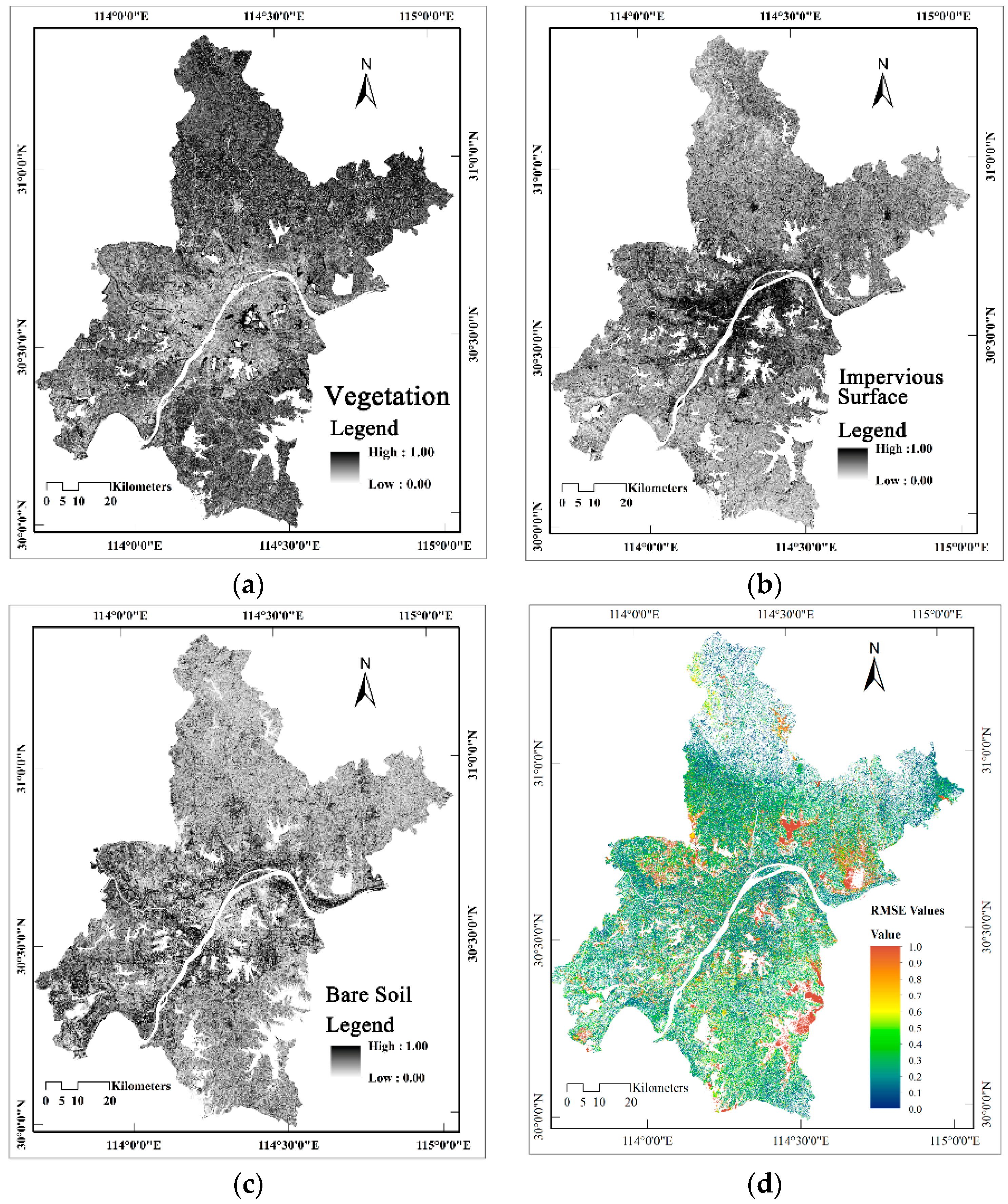
Figure 6.
RMSE statistical result by pixels.
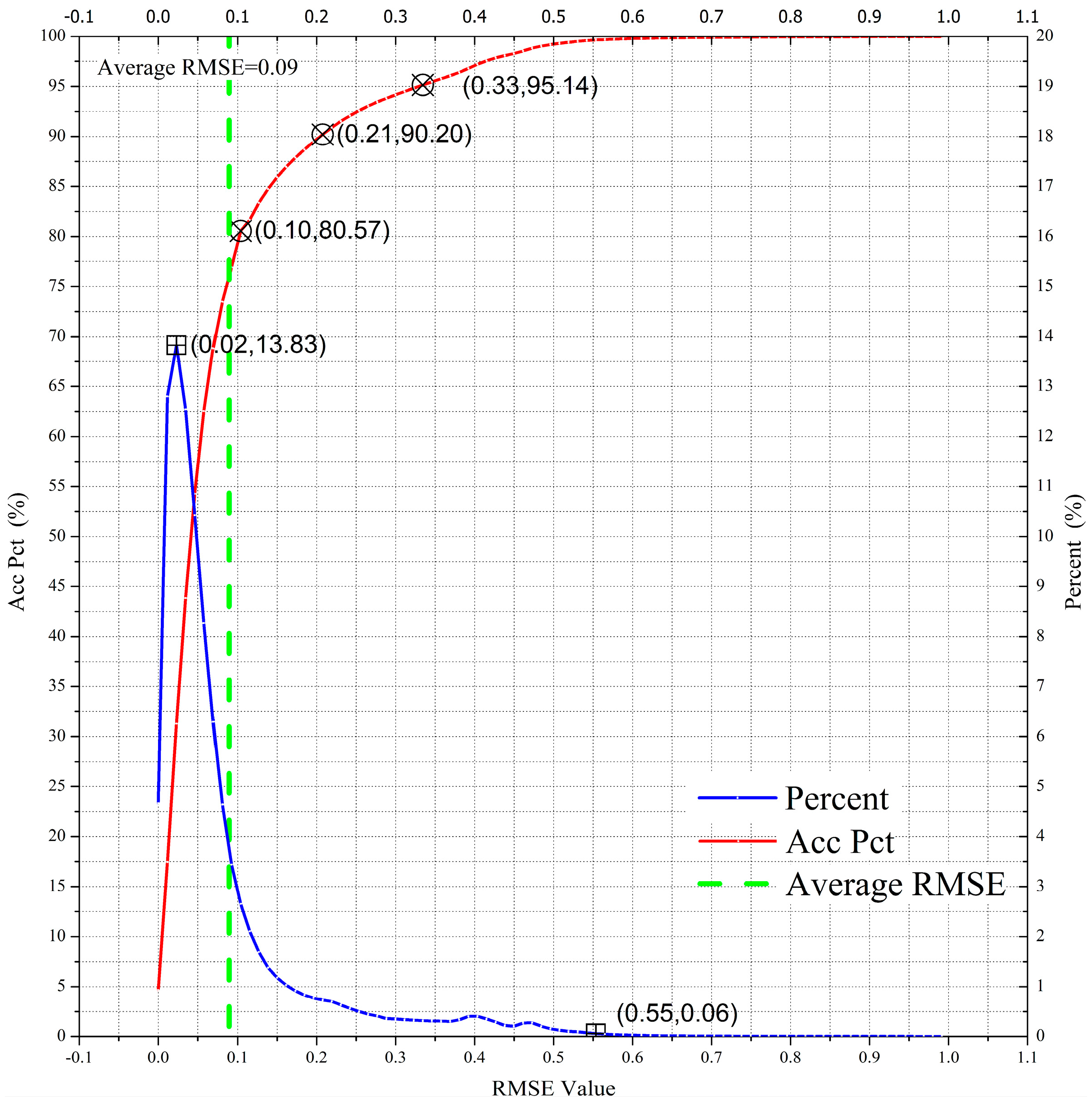
Figure 7.
The classification result of models on the basis of land-cover types of endmember sources.
Figure 7.
The classification result of models on the basis of land-cover types of endmember sources.

Figure 8.
The extraction result for LSBT in the summer of 2013 (TRIS-Band 10).

Figure 9.
TTC for three-endmember fractions overlaid on all the brightness temperature values of the sample points. The transition from blue to red suggests an increase in brightness temperature. (a) The fraction of each sampling point; (b) overlay of all the brightness temperature data.
Figure 9.
TTC for three-endmember fractions overlaid on all the brightness temperature values of the sample points. The transition from blue to red suggests an increase in brightness temperature. (a) The fraction of each sampling point; (b) overlay of all the brightness temperature data.
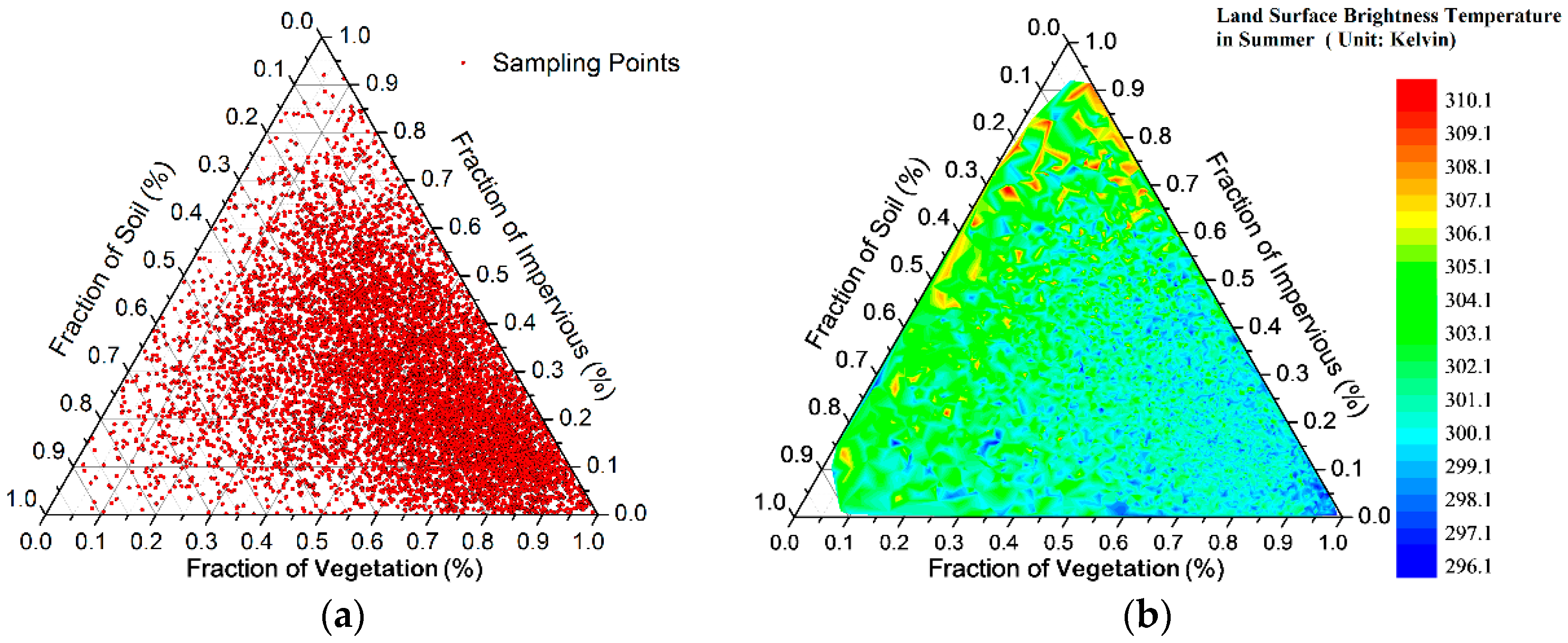
Figure 10.
Scatter diagrams of the land surface brightness temperature and the endmember fraction. (a) Vegetation fraction; (b) impervious surface fraction.
Figure 10.
Scatter diagrams of the land surface brightness temperature and the endmember fraction. (a) Vegetation fraction; (b) impervious surface fraction.


Table 1.
Landsat 8 images used in this study.
| Dates | Path/Row | File Name |
|---|---|---|
| 28 May 2013 | 123/038 | LC81230382013148LGN01 |
| 13 June 2013 | 123/039 | LC81230392013164LGN00 |
| 8 July 2013 | 122/039 | LC81220392013221LGN00 |
Table 2.
The validity of the fitting results of the multiple linear regression analysis.
| Fitted | Adj. R2 | Prob > F | Prob > |t| | ||
|---|---|---|---|---|---|
| Vegetation Fraction | Impervious Fraction | Bare Soil Fraction | |||
| 8# | 0.880 | 1.443 × 10⁻¹⁵ | 1.554 × 10⁻¹⁵ | — | — |
| 9# | 0.902 | 1.11 × 10⁻¹⁶ | — | 0.00 | — |
| 10# | 0.986 | 0.00 | 0.362 | 6.531 × 10⁻⁸ | 0.002 |
© 2017 by the authors. Licensee MDPI, Basel, Switzerland. This article is an open access article distributed under the terms and conditions of the Creative Commons Attribution (CC BY) license (http://creativecommons.org/licenses/by/4.0/).
Share and Cite
MDPI and ACS Style
Chen, T.; Zhang, X.; Niu, R. The Relationship between Urban Land Surface Material Fractions and Brightness Temperature Based on MESMA. Remote Sens. 2017, 9, 532. https://doi.org/10.3390/rs9060532
AMA Style
Chen T, Zhang X, Niu R. The Relationship between Urban Land Surface Material Fractions and Brightness Temperature Based on MESMA. Remote Sensing. 2017; 9(6):532. https://doi.org/10.3390/rs9060532
Chicago/Turabian StyleChen, Tao, Xujia Zhang, and Ruiqing Niu. 2017. "The Relationship between Urban Land Surface Material Fractions and Brightness Temperature Based on MESMA" Remote Sensing 9, no. 6: 532. https://doi.org/10.3390/rs9060532
Note that from the first issue of 2016, this journal uses article numbers instead of page numbers. See further details here.