
Quantifying the Spatiotemporal Trends of Canopy Layer Heat Island (CLHI) and Its Driving Factors over Wuhan, China with Satellite Remote Sensing


1
Jiangsu Center for Collaborative Innovation in Geographical Information Resource Development and Application, Key Laboratory of Virtual Geographic Environment of Ministry of Education, College of Geographic Science, Nanjing Normal University, Nanjing 210023, China
2
School of Remote Sensing and Information Engineering, Wuhan University, Wuhan 430079, China
3
State Key Laboratory of Information Engineering in Surveying, Mapping and Remote Sensing, Wuhan University, Wuhan 430079, China
*
Authors to whom correspondence should be addressed.
Remote Sens. 2017, 9(6), 536; https://doi.org/10.3390/rs9060536
Submission received: 25 March 2017
/
Revised: 13 May 2017
/
Accepted: 24 May 2017
/
Published: 27 May 2017
Abstract
:Canopy layer heat islands (CLHIs) in urban areas are a growing problem. In recent decades, the key issues have been how to monitor CLHIs at a large scale, and how to optimize the urban landscape to mitigate CLHIs. Taking the city of Wuhan as a case study, we examine the spatiotemporal trends of the CLHI along urban-rural gradients, including the intensity and footprint, based on satellite observations and ground weather station data. The results show that CLHI intensity (CLHII) decays exponentially and significantly along the urban-rural gradients, and the CLHI footprint varies substantially and especially in winter. We then quantify the driving factors of the CLHI by establishing multiple linear regression (MLR) models with the assistance of ZY-3 satellite data (with a spatial resolution of 2.5 m), and obtain five main findings: (1) built-up area had a significant positive effect on daily mean CLHII in summer and a negative effect in winter; (2) vegetation had significant inhibiting effects on daily mean CLHII in both summer and winter; (3) absolute humidity has a significant inhibiting effect on daily mean CLHII in summer and a positive effect in winter; (4) anthropogenic heat emissions exacerbated the daily mean CLHII by about 0.19 °C (90% confidence interval −0.06–0.44 °C) on 17 September 2013 and by about 0.06 °C (−0.06–0.19 °C) on 23 January 2014; and (5) if most of the urban area is transformed into roads (i.e., an extreme case), we estimate that the daily mean CLHII would reach 1.41 °C (0.38–2.44 °C) on 17 September 2013 and 0.14 °C (0.08–0.2 °C) on 23 January 2014 in Wuhan metropolitan area. Overall, the results provide new insights into quantifying the CLHI and its driving factors, to enhance our understanding of urban heat islands.
1. Introduction
Urbanization, which refers to a major anthropogenic influence on the earth’s surface, is taking place at an unprecedented rate in China [1]. Concurrently, the world urban population increased from 1.35 billion in 1970 to 3.63 billion in 2011, and is expected to reach 5 billion by 2030 and 6.4 billion by 2050 [2,3]. As a result of the urbanization process, the global area of impervious surfaces is increasing rapidly [4], triggering a series of negative environmental impacts [5]. Among these impacts, the urban heat island (UHI) effect, i.e., the phenomenon of urban areas having higher air/surface temperatures than rural areas, can affect not only local and regional climate [6], but also air quality, water supplies, vegetation phenology, and human health [7,8,9,10]. At present, two main strands of research have evolved for quantifying UHIs: canopy layer heat islands (CLHIs) and surface UHIs (SUHIs). A CLHI is determined by measuring surface air temperature (SAT, usually 2 m) above ground, and a SUHI is determined by land surface temperature (LST) derived from remote sensing data [11]. Generally speaking, most of the existing studies have focused on SUHI analysis [12,13,14,15,16,17,18,19,20], and few studies have addressed SAT retrieval from space for CLHI analysis [21,22,23]. Several studies have reported that SAT can have an impact on human health as a result of affecting human sensible temperature and increasing disease transmission [24,25,26]. Thus, there is a strong impetus to understand CLHI effects.
In contrast to rural areas, several studies have analyzed data obtained from ground weather stations and concluded that urban areas have become significantly warmer (i.e., the CLHI effect) in recent decades [27,28,29,30,31,32]. However, these studies have been limited by the sparse distribution of weather stations [33,34]. Satellite imagery can help to overcome the spatial discontinuity issue of ground weather stations, and has been used to derive LST in many studies [35,36,37,38,39]. Unfortunately, the application of LST to quantify the SUHI effect in large-scale areas is impacted by the limited satellite time-series data and cloud and mist disturbance [40,41,42]. Ho et al. combined satellite observations with ground weather station data to map maximum temperature distributions in urban areas [43], but they did not focus on the studies of CLHI, such as its spatiotemporal trends and driving factors.
As the first attempt, based on meteorological data and satellite remote sensing products, the main objectives of our study are: (1) to examine the spatiotemporal trends of the CLHI, including intensity and footprint; (2) to compare the CLHI and SUHI with regard to intensity, footprint, and spatiotemporal continuity, and to confirm the effectiveness of real-time monitoring of CLHI; and (3) to quantify the driving factors of the CLHI (e.g., absolute humidity, built-up land, vegetation, and anthropogenic heat emissions).
2. Study Area
Wuhan, situated in central China (as shown in Figure 1), covers an area of 8594 km2 and has a population of over 10 million, with the mean annual temperature ranging from 15.8 °C to 17.5 °C [44,45]. As the capital of Hubei province, it is recognized as the industrial base, scientific education base, and transportation center of central China. Its metropolitan area is divided into three parts by the confluence of the Yangtze River and Han River. It has a water area of about 2217 km2, which covers a quarter of the total area. Over the last three decades, Wuhan has experienced rapid urbanization that is similar to that experienced in Shanghai, Beijing, and Guangzhou [46]. Therefore, research into the CLHI is of special significance for this city.
3. Materials and Methods
3.1. Data Preparation
In this study, data for a total of 436 regional automatic weather stations were obtained from the Meteorological Bureau of Hubei Province [47]. The type of automatic weather stations includes ZQZ-A, HY-361, DZZ4 and CAWS600-RT. Temperature and humidity sensors from theses weather stations are installed in the window-shades for preventing from the influence of strong winds, rain and snow. Meteorological data from these stations have measuring accuracies in 0.1 °C and 0.1 hpa for air temperature and vapour pressure, respectively. Among these weather stations, 137 weather stations were situated in the study area (red rectangle in Figure 1), and both vapour pressure and air temperature were recorded by a total of 28 weather stations. Landsat-8 images were obtained for 17 September 2013, and 23 January 2014 [48], with a spatial resolution of 30 m. A digital elevation model (DEM) was obtained with a spatial resolution of approximately 100 m [49]. A “nighttime lights” time series product for 2013 was obtained at a 30 arc second grid [50]. The latest Version-5 MODIS-Terra LST product (MOD11A1) monitored at 10:30 h (daytime) and 22:30 h (nighttime) local solar time with an approximately 1-km spatial resolution was also obtained [51].
3.2. Predicting SAT and Absolute Humidity
In the study conducted by Ho et al. of Greater Vancouver, British Columbia, Canada, it was found that the random forest model could produce a more reasonable map of SAT distribution than ordinary least squares (OLS) regression and support vector machine [43]. Therefore, in our study, the random forest model was used to supplement meteorological monitoring network by estimating the SAT and absolute humidity of 100,000 random points in the study area. Based on supplementary monitoring network, inverse distance weighted method was used to map SAT and absolute humidity. A number of different data layers (14 predictive variables) were derived from the Landsat-8 and DEM data as predictive variables in the random forest model: bands 1–7, bands 10–11, the normalized difference vegetation index (NDVI), the normalized difference built-up index (NDBI), the normalized difference water index (NDWI), the DEM, and the LST. All of the 436 weather stations were used for the calibration and validation of the regression for predicting SAT, and these weather stations were divided into two groups: training (50%) and validation (50%), respectively. Moreover, absolute humidity (α) was determined (in g/m3) using the well-known equation of state for water vapour [52]:
where represents vapour pressure (hPa), and represents air temperature (Kelvin), and equal to . As the same with the mapping of SAT, absolute humidity was divided into two groups including training (70%) and validation (30%), and the spatial pattern was generated by random forest model and inverse distance weighted method.
All the layers, except for the elevation, were derived from the Landsat-8 data. The NDVI is constructed by exploiting the great difference in the spectral reflectance in the near-infrared (which is strongly reflected by vegetation) and red bands (which is absorbed by vegetation):
where NIR is reflectance in the near-infrared (OLI 5) band, and R is reflectance in the red (OLI 4) band.
The NDBI is designed [53], using the reflectance in the near-infrared and short-wave bands for exploiting the built-up areas:
where SWIR is reflectance in the short-wave infrared (OLI 6) band, and NIR is reflectance in the near-infrared (OLI 5) band.
The NDWI is an index designed to quantify vegetation water status [54], by using a weak liquid water absorption band (shortwave-infrared band) and the liquid water intensive band (near-infrared band):
where NIR is reflectance in the near-infrared (OLI 5) band, and SWIR is reflectance in the short-wave infrared (OLI 6) band.
LST was derived by the atmospheric correction method [55], i.e., radiative transfer equation (RTE). A flowchart of the methodology used in this study is given in Figure 2. Next, a regression calibration approach was used to reduce the deviation when quantifying the CLHI owing to the tendency of random forest to “regress towards the mean”. It can make the fitted curve of the scatter diagram of observed versus predicted values become a diagonal line. Finally, the RMSE was used to quantify the magnitude of error. The formulas are as follows:
where represents the observed value, represents the predicted value for the weather station, n represents the total number of weather stations.
3.3. Quantifying the CLHII and Footprint
In this study, to examine the CLHI with regard to the spatiotemporal trends of intensity and footprint, we first defined the urban area and the surrounding buffer zones. A three-step method was used to define the urban area [56]. In view of the concentrated distribution of built-up areas in Wuhan, we extracted the urban border based on visual interpretation. The urban area covered a total of 743 km2 in 2013. Emanating outwards from the urban border to the rural areas, nine buffer zones were generated in ArcGIS 10.2. The area of each buffer zone was equal to the urban area (as shown in Figure 3; the scope of Figure 3 is the “study area” outlined in red in Figure 1). Water bodies and pixels with a relatively higher elevation (more than 50 m) in the urban area were excluded from this analysis because these pixels may have overshadowed the effect of the urbanization on SAT [57].
The intensity represents the magnitude of the CLHI (i.e., the CLHII). In this study, we considered the median of the SAT in the three outermost buffer zones as the rural SAT (i.e., the background temperature), because this was able to reduce the bias caused by the possible outliers among the three outermost buffer zones [58]. We calculated the SAT difference () in each buffer zone and the rural SAT as follows:
where represents the difference between the SAT in and the rural SAT, represents the SAT in , and represents the SAT in the rural area (i.e., the background SAT). Among them, indicates the CLHII in the urban area. A positive value of indicates a CLHI effect, and the opposite indicates a “canopy layer cool island” (CLCI) effect. Therefore, the CLHII is loosely defined as the temperature difference between the urban and rural areas (i.e., ).
The footprint represents the areas significantly affected by the CLHI (i.e., the extent of the CLHI). Previous studies have reported that the strength of the SUHI influence decays exponentially with distance from the perimeter of the urban land cover [9]. However, to our knowledge, few studies have focused on the footprint of CLHI, based on the spatial distribution of SAT in the whole region. Thus, an exponential decay model was applied to assess the trends of in each buffer zone for a single day at an interval of 1 h, in different seasons (summer and winter). The formula is expressed as follows:
where A indicates the maximum SAT difference (close to the CLHII); n represents the numbers of urban zones within the buffern; S represents the decay rate of the CLHII along the urban-rural gradients, and a larger S indicates a smaller footprint of CLHI [58].
However, there is no universally accepted method for defining the SUHI footprint since the varies substantially over time and space [31,42,56,58]. Previous studies have focused on the binary classification of measurement sites as “urban” or “rural”, thereby defining the CLHII [27,28,59], but have not focused on the CLHI footprint. Zhou et al. assumed that the SUHI footprint was the continuous extent emanating outward from the urban center to the rural areas with statistically larger than zero [58]. However, this method fails to calculate the CLHI footprint because SAT is significantly affected by wind, relative to the SUHI footprint. Therefore, we quantified the CLHI footprint as the continuous extent emanating outward from the urban center to the rural areas with the CLHI showing an inverse trend in certain buffer zones (i.e., CLHI: , , , CLCI: , where n represents the CLHI footprint, unit: number of the buffer zone). Batty introduced a graphical representation termed the “rank clock” to examine the trajectories of cities in US [60]. The “rank clock” was used to describe the spatial and temporal variations of size of cities. Based on “rank clock”, we examined the dynamics of CLHI footprint. The circumference represents the time series range from 0:00 to 23:00, and the distance away from the center represents the CLHI footprint.
3.4. Quantifying Potential Drivers of the CLHI
The OLS model has been widely used in the analysis of the SUHI effect [17,61,62]. However, few studies have focused on the drivers of CLHI. The OLS model was thus used to analyze the CLHI effect. Considering the interacting effects of the driving factors of daily mean CLHII, we quantified the relationships between daily mean CLHII and its driving factors (i.e., absolute humidity, built-up land, vegetation, and anthropogenic heat emissions), to gain a better understanding of the CLHI by establishing the multiple linear regression (MLR) model. In this study, the mean values of the driving factors in every buffer zone were used to quantify the relationships with daily mean CLHII. The driving factors of built-up land, vegetation, absolute humidity, and anthropogenic heat emissions were considered as the explanatory variables, and the daily mean CLHII was considered as the response variable to quantify. Specifically, nighttime lights were used as a proxy of anthropogenic heat release (e.g., buildings, industry, and vehicles) in both the urban area and suburbs [42,56,63]. The NDBI was able to describe built-up areas [53]. The NDVI was used to describe the vegetation abundance.
In order to quantify the potential CLHII in different conditions (e.g., a built-up area covered with sparse vegetation) based on the MLR model, we extracted the land-cover types, including bare land, woodland, herbage, building, road, river, and lake, to determine the NDBI, the NDVI, and the absolute humidity of the land cover. We extracted the land cover using the maximum likelihood method and a post-classification process (including majority analysis, clump classes, and sieve classes) implemented in ENVI 5.1. The nighttime lights product was used to extract urban impervious surfaces (threshold set as 20). In the urban area, the classes of road/building and woodland/herbage were distinguished with the assistance of high-resolution remote sensing images (i.e., ZY-3 satellite images with a spatial resolution of 2.5 m) [64,65]. Particularly, land cover map obtained from ZY-3 was used to extract parameter values in the urban area, and based on the land cover map obtained from Landsat-8, we extract the parameter values in the rural area. NDBI and NDVI parameters for building, road, woodland, and herbage are calculated in the urban area to indicate the difference index of reflectance of ground objects. Considering the interaction effect in space, humidity parameters for woodland and herbage are calculated only in rural areas because they can be underestimated when built-up area is covered by dense vegetation. In addition, humidity parameters for building and road are calculated only in urban areas because they can be overestimated when built-up area is covered with sparse vegetation. The parameter values of the NDBI, the NDVI, the absolute humidity, and the digital number (DN) of the nighttime lights were substituted into the equation of the MLR model to quantify potential CLHII.
4. Results
4.1. Data Processing Performance
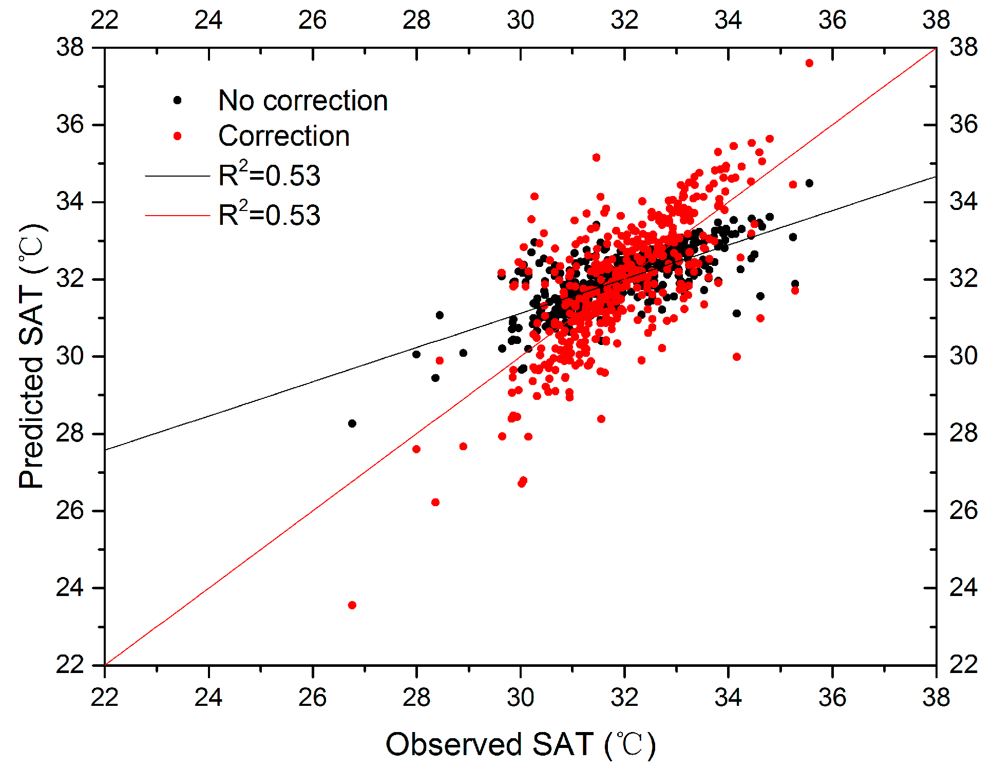
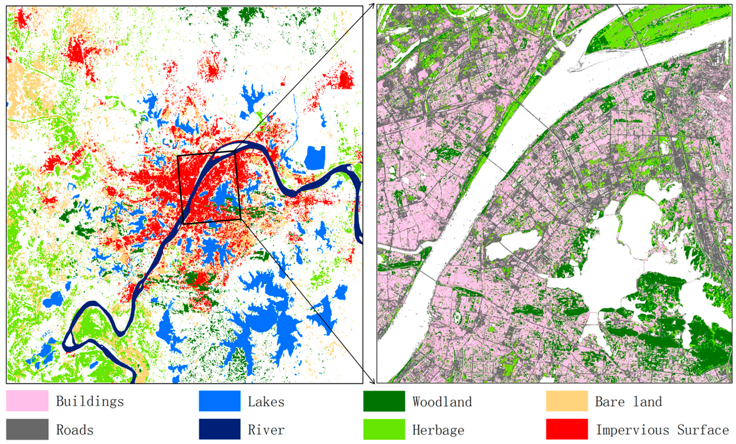
We used a regression calibration approach to reduce the deviation when quantifying the CLHI. This approach makes the fitted curve of the scatter diagram of observed versus predicted values become a diagonal line (an example is shown in Figure 4). The determination coefficients (R2 = 0.53) in this study were superior to the previous study [43]. However, the other roughly 50 % of variance could be affected by many potential factors, such as wind and clouds. The prediction errors (RMSE) at an interval of 1 h are displayed in Figure 5. The daily mean RMSEs were 1.70 °C (SAT in summer), 2.32 °C (SAT in winter), 1.36 g/m3 (absolute humidity in summer) and 0.71 g/m3 (absolute humidity in winter) after correction. The maximum likelihood method (overall accuracy = 88.04%, Kappa coefficient = 0.84) and a post-classification process were used to extract the land-use types in the study area. The classes of road/building and woodland/farmland were distinguished based on high-resolution remote sensing images (i.e., ZY-3 satellite data with a spatial resolution of 2.5 m) in the urban area, and woodland/farmland was distinguished based on Landsat-8 images in the rural area (Figure 6).
4.2. CLHI and SUHI
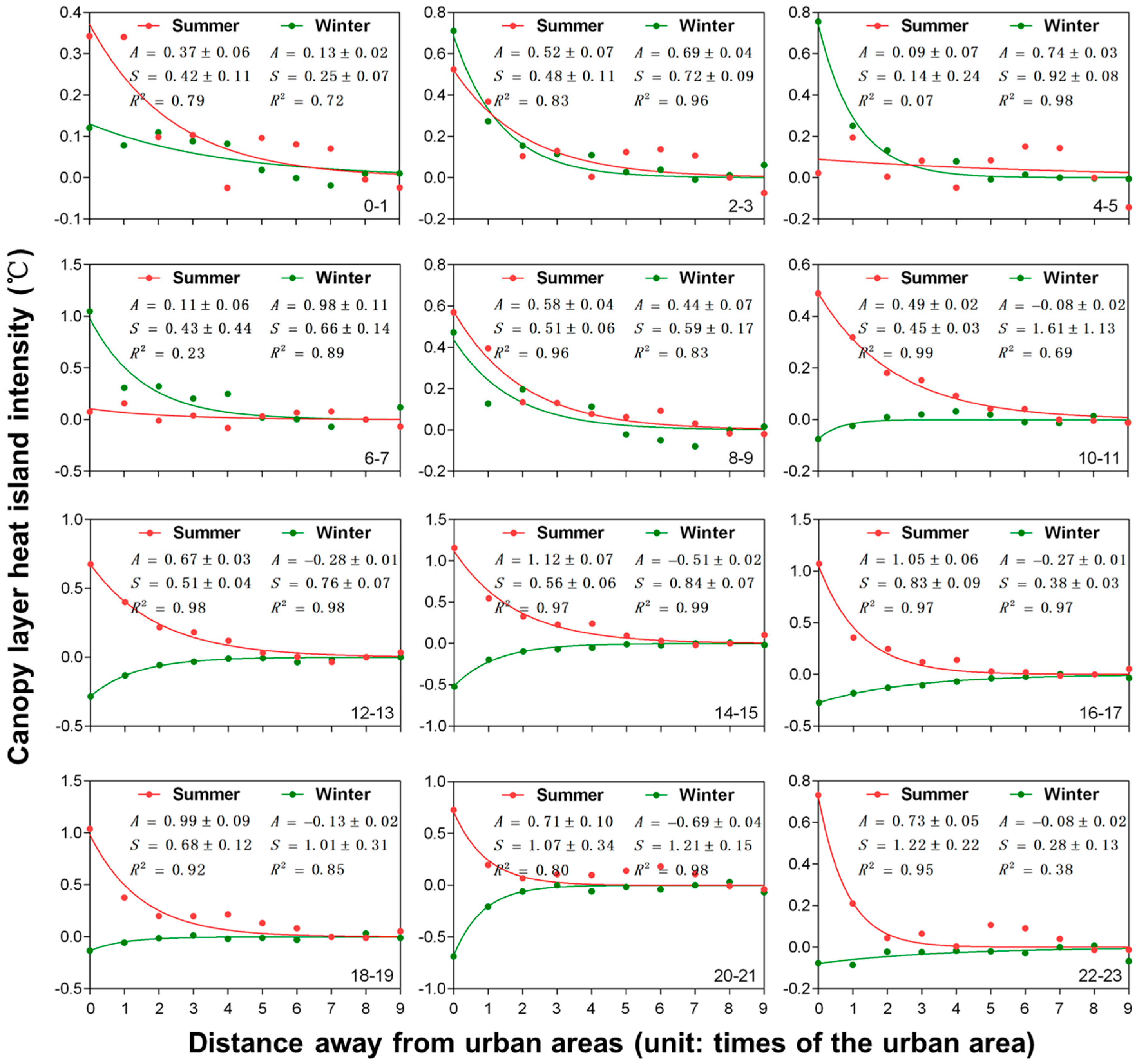
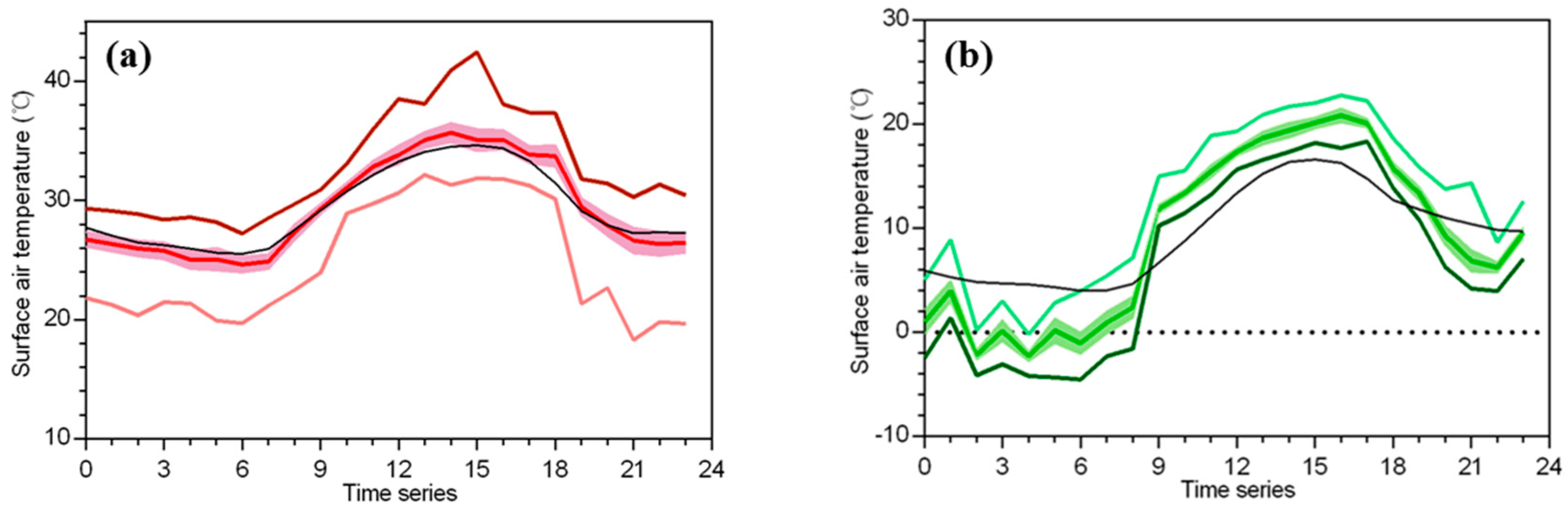
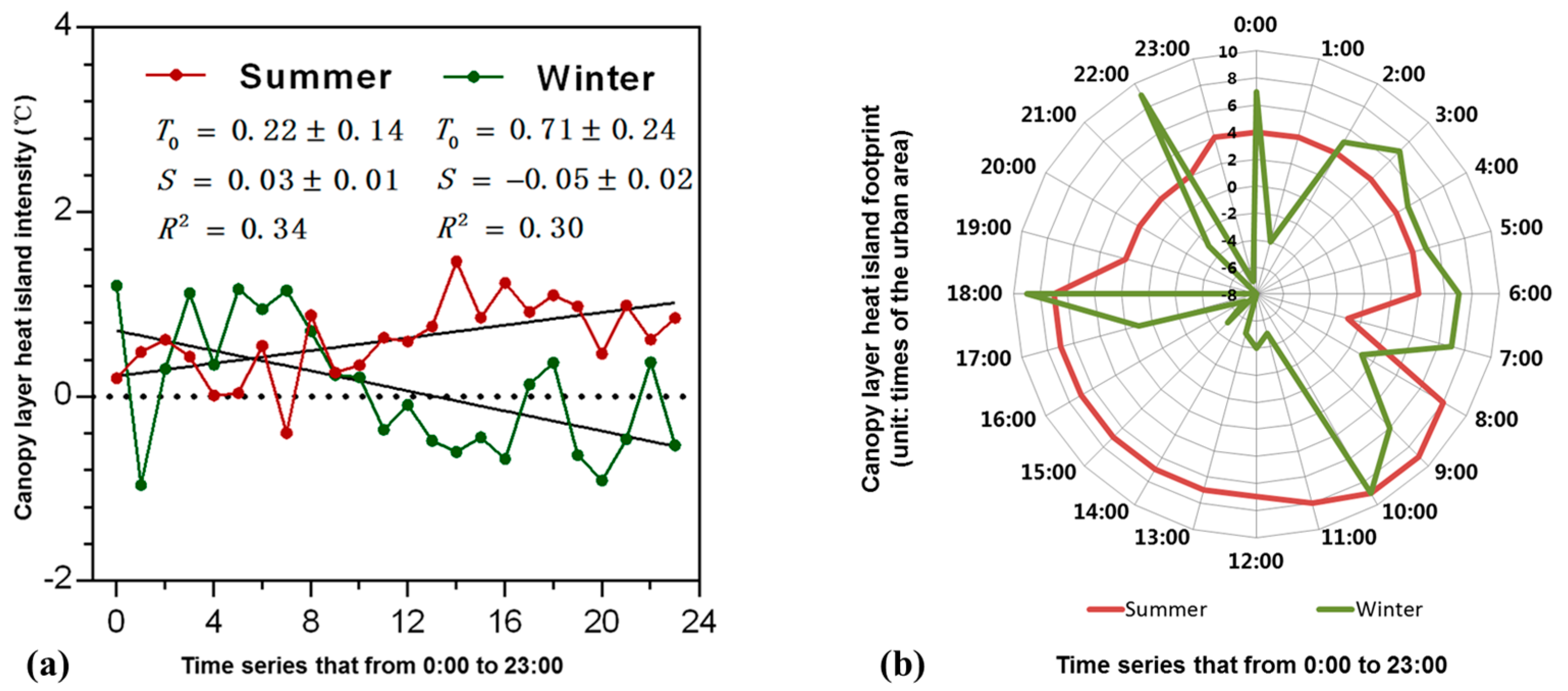
Daily mean SAT is shown in Figure 7. LST derived from Landsat-8 and MODIS-terra is shown in Figure 8. Although the obvious differences that high LST existed in the western part for the LST from MODIS-terra in summer, it would not affect the quantification of SUHI, because the study area mainly covers the eastern part, where the city SUHI is well established. Exponential decay trends of daily mean CLHII and SUHII along the urban-rural (buffer zones 0–9) gradients are given in Figure 9. Particularly, MODIS (Terra) and Landsat-8 OLI/TIRS were used to derive the LST, but the LST obtained from the MOD11A1 product was not available during both daytime and nighttime in winter, because of cloud cover. In addition, exponential decay trends of the CLHI at an interval of 2 h are also given in Figure 10. Based on estimated and observed temperature, the change trends of daily SAT (maximum, mean, and minimum value) are given in Figure 11. The temporal trends of the CLHII were successfully quantified (as shown in Figure 12a). Furthermore, the CLHI footprint was successfully revealed by the rank clock (as shown in Figure 12b).
4.3. Relationships between CLHI and Potential Drivers
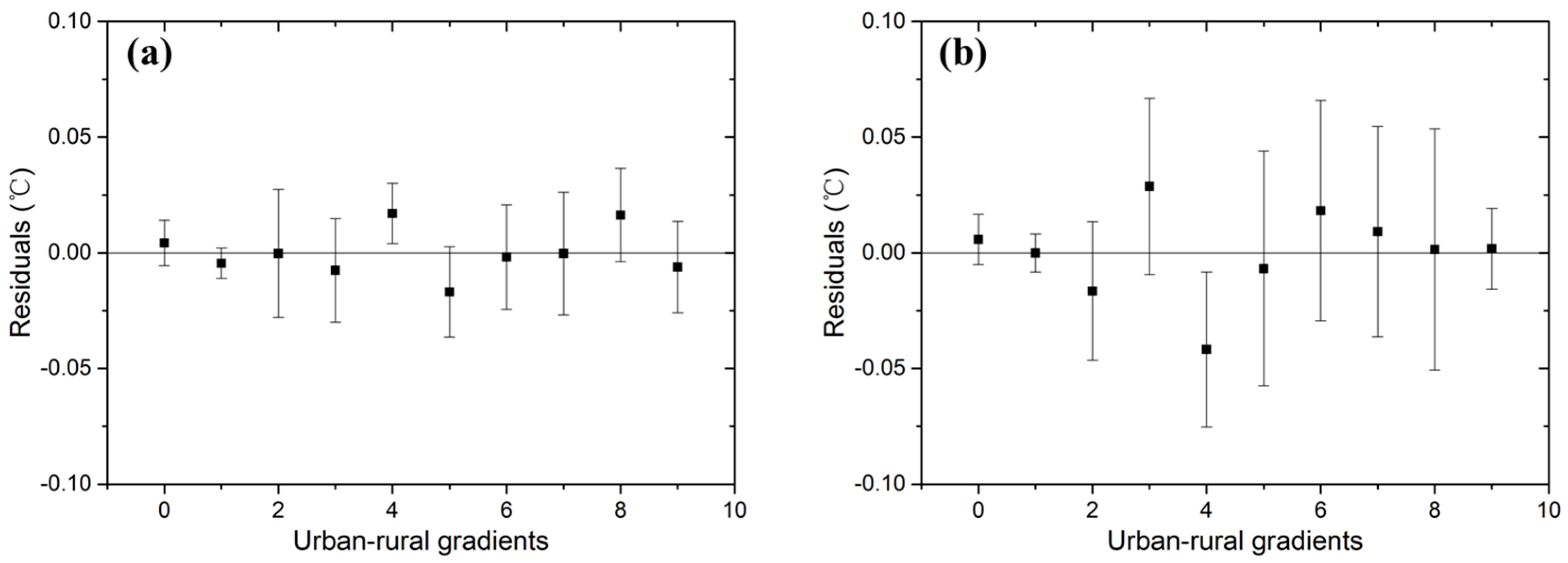
We analyzed the relationships between CLHI and potential drivers based on the mean values of the driving factors and CLHII in every buffer zone. Figure 13 shows single-level relationships between daily mean CLHII and its driving factors quantified by the OLS model. We tried to gain a better understanding of the CLHI by establishing the MLR model. The mean values of the metrics used for quantifying the daily mean CLHII in the different land-cover types are given in Table 1. Estimated correlation coefficients and intervals for every driving factor are given in Table 2. Buffer residuals along the urban-rural (buffer zones 0–9) gradients are shown in Figure 14.
5. Discussion
5.1. Comparison between SUHII and CLHII
SAT were measured in the built-up area (i.e., the red border in Figure 3a) for 17 September 2013, and 23 January 2014. Results showed a difference between observed daily mean values and predicted daily mean values, and we also found large amplitude for predicted values in comparison with observed values, which indicated the limitation of sparse weather stations on monitoring CLHI. A comparison between SUHII and CLHII is given in Table 3. Results indicated that extreme high temperature accompanied by strong CLHI occurred during 14:00–15:00, and low temperature accompanied by CLHI effect at 7:00 in summer, and the CLHI and CLCI effects alternately appeared in winter over Wuhan built-up area. In addition, the surface urban cool island (SUCI) effect was not detected based on the satellite data, and the SUHII measured at 10:30, 10:58, and 22:30 was greater than the maximum CLHII (1.42 °C at 14:00). Results indicated obvious difference between SUHII and CLHII for quantifying the magnitude of UHI effect, since the former represents the SAT difference, but the latter is the LST difference between urban and rural areas. Comparatively speaking, the analysis of the CLHII helps with the understanding of global temperature change in different cities, especially where the metropolis area has the strongest CLHII accounting for global warming.
5.2. Spatiotemporal Trends of the CLHI
We found that not only did the SUHI footprint show exponential decay and significantly, but also the CLHI footprint, for both summer and winter, signifying the difference between the radiative energy absorbed at the surface and the anthropogenic heating released in urban areas. It hence caused uneven incoming energy radiated into the atmosphere accompanied by CLHI (or CLCI) effect occurring. CLHI showed increasing trends in 17 September, 2013 and decreasing trends in 23 January 2014. In summer, the CLHI footprint was stable and varied from −1 to 9 times the urban area (standard deviation (SD) = 2.62, where −1 indicates a CLCI). The mean CLHI footprint was 5.08 times the urban area, and the mean footprint was 7.55 times the urban area from 8:00 to 18:00, as a result of solar radiation. In winter, the CLHI footprint varied substantially and ranged from −8 to 9 times the urban area (SD = 6.43). The mean CLHI footprint in winter was only 0.58 times the urban area. In contrast, the CLHI effect tended to occur in summer. Overall, the time-series analysis at an interval of 1 h allows us to continuously monitor the CLHI effect, and helps with the understanding of the spatiotemporal trends of the CLHI.
5.3. Single-Level Relationships Quantified with the OLS Model
The results of the OLS model signified that NDBI (summer: R2 = 0.94, p < 0.01; winter: R2 = 0.31, p = 0.093) and nighttime lights (summer: R2 = 0.94, p < 0.01; winter: R2 = 0.60, p < 0.01) consistently exhibited a positive effect on the daily mean CLHII, and NDVI (summer: R2 = 0.96, p < 0.01; winter: R2 = 0.62, p < 0.01), and absolute humidity (summer: R2 = 0.94, p < 0.01; winter: R2 = 0.29, p = 0.11) consistently showed a negative effect in both summer and winter. We found that these driving factors were significantly correlated with the daily mean CLHII in summer (R2 > 0.90). Conversely, the results showed a decreased correlation in winter (R2 < 0.65), which is mostly due to the substantial variation of SAT over time and space in winter. Especially for the contribution of NDBI and absolute humidity to CLHI, insignificant correlations existed in summer and winter, respectively. According to the single-level relationships quantified with the OLS model, we thus concluded that anthropogenic heat emissions (e.g., buildings, industry, and vehicles) have significant positive effects on CLHI, and vegetation has significant negative effects in both summer and winter. Built-up area has significant positive effects on CLHI, and absolute humidity has significant negative effects in summer. However, both the contribution of built-up area and absolute humidity were not significant in winter based on the analysis of OLS model.
5.4. Interacting Effects Quantified with the MLR Model
Absolute humidity had a significant inhibiting effect on daily mean CLHII in summer (estimated coefficients = −0.26) and a positive effect in winter (estimated coefficients = 0.9). Fountain is suggested to mitigate the CLHI in summer because of vast area of waters. Vegetation had significant inhibiting effects on daily mean CLHII in both summer (estimated coefficients = −8.13) and winter (estimated coefficients = −4.56). Built-up area had a significant positive effect on daily mean CLHII in summer (estimated coefficients = −10.83) and a negative effect in winter (estimated coefficients = 3.04). Anthropogenic heat emissions (e.g., buildings, industry, and vehicles) have positive effects in both summer (estimated coefficients = 0.003) and winter (estimated coefficients = 0.001). The factories producing high heat emissions are suggested to be pushed to the outskirts, and public transport is promoted in metropolitan area for mitigating the CLHI in Wuhan, because it is regarded as the industrial base and transportation center of central China. Particularly, based on MLR model, the correlation with daily mean CLHII for NDBI and absolute humidity was contrary to the results of OLS model in winter. However, the result of MLR model was significant (R2 = 0.89, p = 0.011) and OLS models were not significant for NDBI (R2 = 0.31, p > 0.05) and absolute humidity (R2 = 0.29, p > 0.05) in winter. Therefore, the results underscores the importance of quantifying the interacting effects of the driving factors of the CLHI based on the MLR model rather than the OLS model.
We calculated the daily mean CLHII in different conditions to understand the contribution of the different driving factors to CLHI. In summer, when we set absolute humidity as 17.25 g/m3, the NDBI as −0.04, the NDVI as 0.13, and the DN of nighttime lights as 63 (i.e., most of the land use was physically transformed into buildings in the urban area; refer to Table 1 for the parameter values and Table 2 for the estimated correlation coefficients), the daily mean CLHII was expected to reach 1.30 °C (90% confidence interval 0.38–2.22 °C). Comparably, when most of the land use was transformed into roads, the daily mean CLHII was expected to reach 1.41 °C (0.38–2.44 °C). Conversely, the daily mean CLHII was expected to reduce to 0.27 °C (−0.04–0.57 °C) for the urban area covered by grassland. In addition, when the urban area was covered by woodlands, the daily mean CLHII was expected to reduce to 0.21 °C (0.03–0.38 °C). In winter, the daily mean CLHII was expected to reach 0.17 °C (0.04–0.3 °C), 0.14 °C (0.08–0.2 °C), 0.03 °C (−0.04–0.09 °C), and 0.34 °C (0.05–0.64 °C) in the above conditions, respectively. Therefore, the contribution of roads to the CLHI is greater than buildings, and the mitigation of the CLHI through afforestation is superior to planting grass in summer. In winter, the contribution of roads to the CLHI is less than buildings, and the mitigation of the extreme low-temperature weather through afforestation is superior to planting grass. Therefore, planting trees and avoiding the construction of wide roads are suggested to mitigate the CLHI. In addition, it was found that anthropogenic heat emissions exacerbated the daily mean CLHII by about 0.19 °C (−0.06–0.44 °C) on 17 September 2013. However, anthropogenic heat emissions exacerbated daily mean CLHII 0.06 °C (−0.06–0.19 °C) on 23 January 2014.
6. Conclusions
Quantifying SUHI is significantly impacted by the limited satellite time-series data and cloud and mist disturbance, and quantifying CLHI is significantly limited by sparse meteorological monitoring network. The findings of this study indicate that quantifying the CLHI effects based on satellite observations as well as ground weather station data can enable us to overcome the issues of spatial discontinuity and the low temporal resolution, and also confirm the effectiveness of real-time monitoring of CLHI.
The CLHI effect decays exponentially and significantly along urban-rural gradients. Regarding hourly CLHII, the trends of the exponential decay are more significant in winter. Conversely, the daily mean CLHII decays exponentially, but it is more significant in summer than in winter, which is mostly attributed to the substantial variation over time and space (i.e., CLHI and CLCI effects alternating) in winter, signifying the difference in the radiative energy absorbed at the surface and anthropogenic heating released in urban areas compared to rural areas.
This study underscores the importance of quantifying the interacting effects of the driving factors of the CLHI based on the MLR model rather than the OLS model. Additionally, the ZY-3 satellite data enable us to obtain more subtle information. We concluded that vegetation had significant inhibiting effects on daily mean CLHII in both summer and winter. Absolute humidity has a significant inhibiting effect on daily mean CLHII in summer and a positive effect in winter. Built-up area had a significant positive effect on daily mean CLHII in summer and a negative effect in winter. Anthropogenic heat emissions (e.g., buildings, industry, and vehicles) have positive effects in both summer and winter. Therefore, planting trees and fountain, and reducing the emissions from industry and vehicle (e.g., the factories producing high heat emissions are suggested to be pushed to the outskirts, and public transport is promoted in metropolitan area) are suggested to mitigate the CLHI in the city of Wuhan.
Acknowledgments
This work was supported by the China National Science Fund for Excellent Young Scholars under grant 41522110, by the National Key Research and Development Plan under grant 2016YFB0501403, and by the Foundation for the Author of National Excellent Doctoral Dissertation, China, under grant 201348.
Author Contributions
Long Li and Xin Huang Conceived and designed the experiments; Long Li Collected, prepared, processed, analyzed data, interpreted and discussed the results, and wrote the manuscript; Xin Huang Supplied climatological data and contributed in the results interpretation, manuscript editing, and supervised all the work that has been done by the first author; Jiayi Li Provided suggestion and comments for results interpretation and manuscript editing; Dawei Wen Supplied ZY-3 satellite data and contributed with manuscript editing before submission. All authors reviewed the manuscript.
Conflicts of Interest
The authors declare that there is no conflict of interest.
Abbreviations
| UHI | Urban heat island |
| CLHI | Canopy layer heat island |
| CLHII | Canopy layer heat island intensity |
| SUHI | Surface urban heat island |
| SUHII | Surface urban heat island intensity |
| CLCI | Canopy layer cool island |
| SUCI | Surface urban cool island |
| SAT | Surface air temperature |
| LST | Land surface temperature |
| NDVI | Normalized difference vegetation index |
| NDBI | Normalized difference built-up index |
| NDWI | Normalized difference water index |
| DEM | Digital elevation model |
| DN | Digital number |
| MLR | Multiple linear regression |
| OLS | Ordinary least squares |
References
- Bai, X.; Shi, P.; Liu, Y. Realizing China’s urban dream. Nature 2014, 509, 158–160. [Google Scholar] [CrossRef] [PubMed]
- Angel, S.; Parent, J.; Civco, D.L.; Blei, A.; Potere, D. The dimensions of global urban expansion: Estimates and projections for all countries, 2000–2050. Prog. Plan. 2011, 75, 53–107. [Google Scholar] [CrossRef]
- Heilig, G.K. World Urbanization Prospects: The 2011 Revision; United Nations: New York, NY, USA, 2012. [Google Scholar]
- Elvidge, C.D.; Tuttle, B.T.; Sutton, P.S.; Baugh, K.E.; Howard, A.T.; Milesi, C. Global distribution and density of constructed impervious surfaces. Sensors 2017, 7, 1962–1979. [Google Scholar] [CrossRef]
- Valerio, Q.; Anna, B.; Francesco, C.; Diego, G.; Dalila, R.; Piermaria, C. Monitoring land take by point sampling: Pace and dynamics of urban expansion in the metropolitan city of Rome. Landsc. Urban Plan. 2015, 143, 126–133. [Google Scholar] [CrossRef]
- Grimm, N.B.; Faeth, S.H.; Golubiewski, N.E.; Redman, C.L.; Wu, J.; Bai, X. Global change and the ecology of cities. Science 2008, 319, 756–760. [Google Scholar] [CrossRef] [PubMed]
- Platt, R.H.; Rowntree, R.A.; Muick, P.C. The Ecological City: Preserving and Restoring Urban Biodiversity; University of Massachusetts Press: Amherst, MA, USA, 1994. [Google Scholar]
- Gober, P.; Wentz, E.A.; Lant, T.; Tschudi, M.K.; Kirkwood, C.W. Watersim: A simulation model for urban water planning in phoenix, Arizona, USA. Environ. Plan. B Plan. Des. 2011, 38, 197–215. [Google Scholar] [CrossRef]
- Zhang, X.; Friedl, M.A.; Schaaf, C.B.; Strahler, A.H.; Schneider, A. The footprint of urban climates on vegetation phenology. Geophys. Res. Lett. 2004, 31, 179–206. [Google Scholar] [CrossRef]
- Harvell, C.D.; Mitchell, C.E.; Ward, J.R.; Altizer, S.; Dobson, A.P.; Ostfeld, R.S. Climate warming and disease risks for terrestrial and marine biota. Science 2002, 296, 2158–2162. [Google Scholar] [CrossRef] [PubMed]
- Schwarz, N.; Lautenbach, S.; Seppelt, R. Exploring indicators for quantifying surface urban heat islands of European cities with MODIS land surface temperatures. Remote Sens. Environ. 2011, 115, 3175–3186. [Google Scholar] [CrossRef]
- Weng, Q.; Lu, D.; Schubring, J. Estimation of land surface temperature—Vegetation abundance relationship for urban heat island studies. Remote Sens. Environ. 2004, 89, 467–483. [Google Scholar] [CrossRef]
- Xiong, Y.; Huang, S.; Chen, F.; Ye, H.; Wang, C.; Zhu, C. The impacts of rapid urbanization on the thermal environment: A remote sensing study of Guangzhou, South China. Remote Sens. 2012, 4, 2033–2056. [Google Scholar] [CrossRef]
- Guo, G.; Wu, Z.; Xiao, R.; Chen, Y.; Liu, X.; Zhang, X. Impacts of urban biophysical composition on land surface temperature in urban heat island clusters. Landsc. Urban Plan. 2015, 135, 1–10. [Google Scholar] [CrossRef]
- Zheng, B.; Myint, S.W.; Fan, C. Spatial configuration of anthropogenic land cover impacts on urban warming. Landsc. Urban Plan. 2014, 130, 104–111. [Google Scholar] [CrossRef]
- Connors, J.P.; Galletti, C.S.; Chow, W.T.L. Landscape configuration and urban heat island effects: Assessing the relationship between landscape characteristics and land surface temperature in phoenix, Arizona. Landsc. Ecol. 2013, 28, 271–283. [Google Scholar] [CrossRef]
- Du, S.; Xiong, Z.; Wang, Y.C.; Guo, L. Quantifying the multilevel effects of landscape composition and configuration on land surface temperature. Remote Sens. Environ. 2016, 178, 84–92. [Google Scholar] [CrossRef]
- Chun, B.; Guldmann, J.M. Spatial statistical analysis and simulation of the urban heat island in high-density central cities. Landsc. Urban Plan. 2014, 125, 76–88. [Google Scholar] [CrossRef]
- Yuan, F.; Bauer, M.E. Comparison of impervious surface area and normalized difference vegetation index as indicators of surface urban heat island effects in Landsat imagery. Remote Sens. Environ. 2007, 106, 375–386. [Google Scholar] [CrossRef]
- Sobrino, J.A.; Oltra-Carrió, R.; Sòria, G.; Bianchi, R.; Paganini, M. Impact of spatial resolution and satellite overpass time on evaluation of the surface urban heat island effects. Remote Sens. Environ. 2012, 117, 50–56. [Google Scholar] [CrossRef]
- Fabrizi, R.; Santis, A.D.; Gomez, A. Satellite and ground-based sensors for the urban heat island analysis in the city of Madrid. Remote Sens. 2011, 2, 349–352. [Google Scholar]
- Pichierri, M.; Bonafoni, S.; Biondi, R. Satellite air temperature estimation for monitoring the canopy layer heat island of Milan. Remote Sens. Environ. 2012, 127, 130–138. [Google Scholar] [CrossRef]
- Anniballe, R.; Bonafoni, S.; Pichierri, M. Spatial and temporal trends of the surface and air heat island over Milan using MODIS data. Remote Sens. Environ. 2014, 150, 163–171. [Google Scholar] [CrossRef]
- Koken, P.J.; Piver, W.T.; Ye, F.; Elixhauser, A.; Olsen, L.M.; Portier, C.J. Temperature, air pollution, and hospitalization for cardiovascular diseases among elderly people in Denver. Environ. Health Perspect. 2003, 111, 1312–1317. [Google Scholar] [CrossRef] [PubMed]
- Chen, K.; Huang, L.; Zhou, L.; Ma, Z.; Bi, J.; Li, T. Spatial analysis of the effect of the 2010 heat wave on stroke mortality in Nanjing, China. Sci. Rep. 2015, 5, 10816. [Google Scholar] [CrossRef]
- Xu, Z.; Liu, Y.; Ma, Z.; Sam, T.G.; Hu, W.; Tong, S. Assessment of the temperature effect on childhood diarrhea using satellite imagery. Sci. Rep. 2014, 4, 5389. [Google Scholar] [CrossRef]
- Ren, G.Y.; Chu, Z.Y.; Chen, Z.H.; Ren, Y.Y. Implications of temporal change in urban heat island intensity observed at Beijing and Wuhan stations. Geophys. Res. Lett. 2007, 34, 89–103. [Google Scholar] [CrossRef]
- Sun, Y.; Zhang, X.; Ren, G.; Zwiers, F.W.; Hu, T. Contribution of urbanization to warming in China. Nat. Clim. Chang. 2016, 6, 706–709. [Google Scholar] [CrossRef]
- Campra, P.; Millstein, D. Mesoscale climatic simulation of surface air temperature cooling by highly reflective greenhouses in se Spain. Environ. Sci. Technol. 2013, 47, 12284–12290. [Google Scholar] [CrossRef] [PubMed]
- Parker, D.E. Urban heat island effects on estimates of observed climate change. Wiley Interdiscip. Rev. Clim. Chang. 2010, 1, 123–133. [Google Scholar] [CrossRef]
- Zhao, L.; Lee, X.; Smith, R.B.; Oleson, K. Strong contributions of local background climate to urban heat islands. Nature 2014, 511, 216–219. [Google Scholar] [CrossRef] [PubMed]
- Li, Q.; Zhang, H.; Liu, X.; Huang, J. Urban heat island effect on annual mean temperature during the last 50 years in China. Theor. Appl. Clim. 2004, 79, 165–174. [Google Scholar] [CrossRef]
- Ren, G.; Zhou, Y.; Chu, Z.; Zhou, J.; Zhang, A.; Guo, J. Urbanization effects on observed surface air temperature trends in north China. J. Clim. 2008, 21, 1333–1348. [Google Scholar] [CrossRef]
- Yang, X.; Hou, Y.; Chen, B. Observed surface warming induced by urbanization in east China. J. Geophys. Res. Atmos. 2011, 116, 263–294. [Google Scholar] [CrossRef]
- Sobrino, J.A.; Jiménez-Muñoz, J.C.; Paolini, L. Land surface temperature retrieval from Landsat TM 5. Remote Sens. Environ. 2004, 90, 434–440. [Google Scholar] [CrossRef]
- Wan, Z.; Dozier, J. A generalized split-window algorithm for retrieving land-surface temperature from space. IEEE Trans. Geosci. Remote Sens. 1996, 34, 892–905. [Google Scholar]
- Wan, Z. New refinements and validation of the MODIS land-surface temperature/emissivity products. Remote Sens. Environ. 2008, 140, 59–74. [Google Scholar] [CrossRef]
- Wang, A.S.; He, L. Practical split-window algorithm for retrieving land surface temperature over agricultural areas from aster data. J. Appl. Remote Sens. 2014, 8, 5230–5237. [Google Scholar] [CrossRef]
- Li, Z.L.; Tang, B.H.; Wu, H.; Ren, H.; Yan, G.; Wan, Z.; Trigo, I.F.; Sobrino, J.A. Satellite-derived land surface temperature: Current status and perspectives. Remote Sens. Environ. 2013, 131, 14–37. [Google Scholar] [CrossRef]
- Cai, G.; Xue, M.D.Y. Monitoring of urban heat island effect in Beijing combining aster and tm data. Int. J. Remote Sens. 2011, 32, 1213–1232. [Google Scholar] [CrossRef]
- Shen, H.; Huang, L.; Zhang, L.; Wu, P.; Zeng, C. Long-term and fine-scale satellite monitoring of the urban heat island effect by the fusion of multi-temporal and multi-sensor remote sensed data: A 26-year case study of the city of Wuhan in China. Remote Sens. Environ. 2016, 172, 109–125. [Google Scholar] [CrossRef]
- Peng, S.; Piao, S.; Ciais, P.; Friedlingstein, P.; Ottle, C.; Bréon, F.M.; Nan, H.; Zhou, L.; Myneni, R.B. Surface urban heat island across 419 global big cities. Environ. Sci. Technol. 2012, 46, 696–703. [Google Scholar] [CrossRef] [PubMed]
- Ho, H.C.; Knudby, A.; Sirovyak, P.; Xu, Y.; Hodul, M.; Henderson, S.B. Mapping maximum urban air temperature on hot summer days. Remote Sens. Environ. 2014, 154, 38–45. [Google Scholar] [CrossRef]
- Han, Y.H.; Li, S.J.; Zheng, Y.L. Predictors of nutritional status among community-dwelling older adults in Wuhan, China. Public Health Nutr. 2009, 12, 1189–1196. [Google Scholar] [CrossRef] [PubMed]
- Qian, Z.; He, Q.; Lin, H.M.; Kong, L.; Liao, D.; Dan, J. Association of daily cause-specific mortality with ambient particle air pollution in Wuhan, China. Environ. Res. 2007, 105, 380–389. [Google Scholar] [CrossRef] [PubMed]
- Wu, H.; Ye, L.P.; Shi, W.Z.; Clarke, K.C. Assessing the effects of land use spatial structure on urban heat islands using HJ-1b remote sensing imagery in Wuhan, China. Int. J. Appl. Earth Obs. Geoinf. 2014, 32, 67–78. [Google Scholar] [CrossRef]
- Meteorological Bureau of Hubei Province. Available online: http://www.hbqx.gov.cn/index.action (accessed on 26 May 2017).
- USGS (United States Geological Survey). Available online: http://glovis.usgs.gov/ (accessed on 26 May 2017).
- The CGIAR Consortium for Spatial Information (CGIAR-CSI) SRTM 90m DEM Digital Elevation Database. Available online: http://srtm.csi.cgiar.org/SELECTION/inputCoord.asp (accessed on 26 May 2017).
- NOAA (National Oceanic and Atmospheric Administration). Version 4 DMSP-OLS Nighttime Lights Time Series. Available online: http://ngdc.noaa.gov/eog/dmsp/downloadV4composites.html (accessed on 26 May 2017).
- LAADS DAAC. Available online: https://ladsweb.nascom.nasa.gov/ (accessed on 26 May 2017).
- Tomasi, C.; Petkov, B.H.; Benedetti, E. Annual cycles of pressure, temperature, absolute humidity and precipitable water from the radiosoundings performed at dome c, antarctica, over the 2005–2009 period. Antarct. Sci. 2012, 24, 637–658. [Google Scholar] [CrossRef]
- Zha, Y.; Gao, J.; Ni, S. Use of normalized difference built-up index in automatically mapping urban areas from tm imagery. Int. J. Remote Sens. 2003, 24, 583–594. [Google Scholar] [CrossRef]
- Maki, M.; Ishiahra, M.; Tamura, M. Estimation of leaf water status to monitor the risk of forest fires by using remotely sensed data. Remote Sens. Environ. 2004, 90, 441–450. [Google Scholar] [CrossRef]
- Barsi, J.A.; Schott, J.R.; Palluconi, F.D.; Hook, S.J. Validation of a web-based atmospheric correction tool for single thermal band instruments. Proc. SPIE 2005. [Google Scholar] [CrossRef]
- Zhou, D.; Zhao, S.; Liu, S.; Zhang, L.; Chao, Z. Surface urban heat island in China’s 32 major cities: Spatial patterns and drivers. Remote Sens. Environ. 2014, 152, 51–61. [Google Scholar] [CrossRef]
- Zhou, D.; Zhao, S.; Liu, S.; Zhang, L. Spatiotemporal trends of terrestrial vegetation activity along the urban development intensity gradient in China’s 32 major cities. Sci. Total Environ. 2014, 488–489, 136–145. [Google Scholar] [CrossRef] [PubMed]
- Zhou, D.; Zhao, S.; Zhang, L.; Sun, G.; Liu, Y. The footprint of urban heat island effect in China. Sci. Rep. 2015, 5, 11160. [Google Scholar] [CrossRef] [PubMed]
- Ren, G.; Zhou, Y. Urbanization effect on trends of extreme temperature indices of national stations over mainland China, 1961–2008. J. Clim. 2014, 27, 2340–2360. [Google Scholar] [CrossRef]
- Batty, M. Rank clocks. Nature 2006, 444, 592–596. [Google Scholar] [CrossRef] [PubMed]
- Zhou, W.; Qian, Y.; Li, X.; Li, W.; Han, L. Relationships between land cover and the surface urban heat island: Seasonal variability and effects of spatial and thematic resolution of land cover data on predicting land surface temperatures. Landsc. Ecol. 2014, 29, 153–167. [Google Scholar] [CrossRef]
- Zhou, W.; Huang, G.; Cadenasso, M.L. Does spatial configuration matter? Understanding the effects of land cover pattern on land surface temperature in urban landscapes. Landsc. Urban Plan. 2011, 102, 54–63. [Google Scholar] [CrossRef]
- Sailor, D.J. A review of methods for estimating anthropogenic heat and moisture emissions in the urban environment. Int. J. Clim. 2011, 31, 189–199. [Google Scholar] [CrossRef]
- Huang, X.; Lu, Q.; Zhang, L. A multi-index learning approach for classification of high-resolution remotely sensed images over urban areas. ISPRS J. Photogramm. Remote Sens. 2014, 90, 36–48. [Google Scholar] [CrossRef]
- Huang, X.; Lu, Q.; Zhang, L.; Plaza, A. New postprocessing methods for remote sensing image classification: A systematic study. IEEE Trans. Geosci. Remote Sens. 2014, 52, 7140–7159. [Google Scholar] [CrossRef]
Figure 1.
Study area, showing the location of the city of Wuhan in central China and the locations of the 436 weather stations. All of the weather stations were used for mapping the SAT; the 28 weather stations recording vapour pressure and SAT data were used to predict the absolute humidity. The acquisition times of the multi-temporal satellite observations and ground weather station data are 17 September 2013, and 23 January 2014.
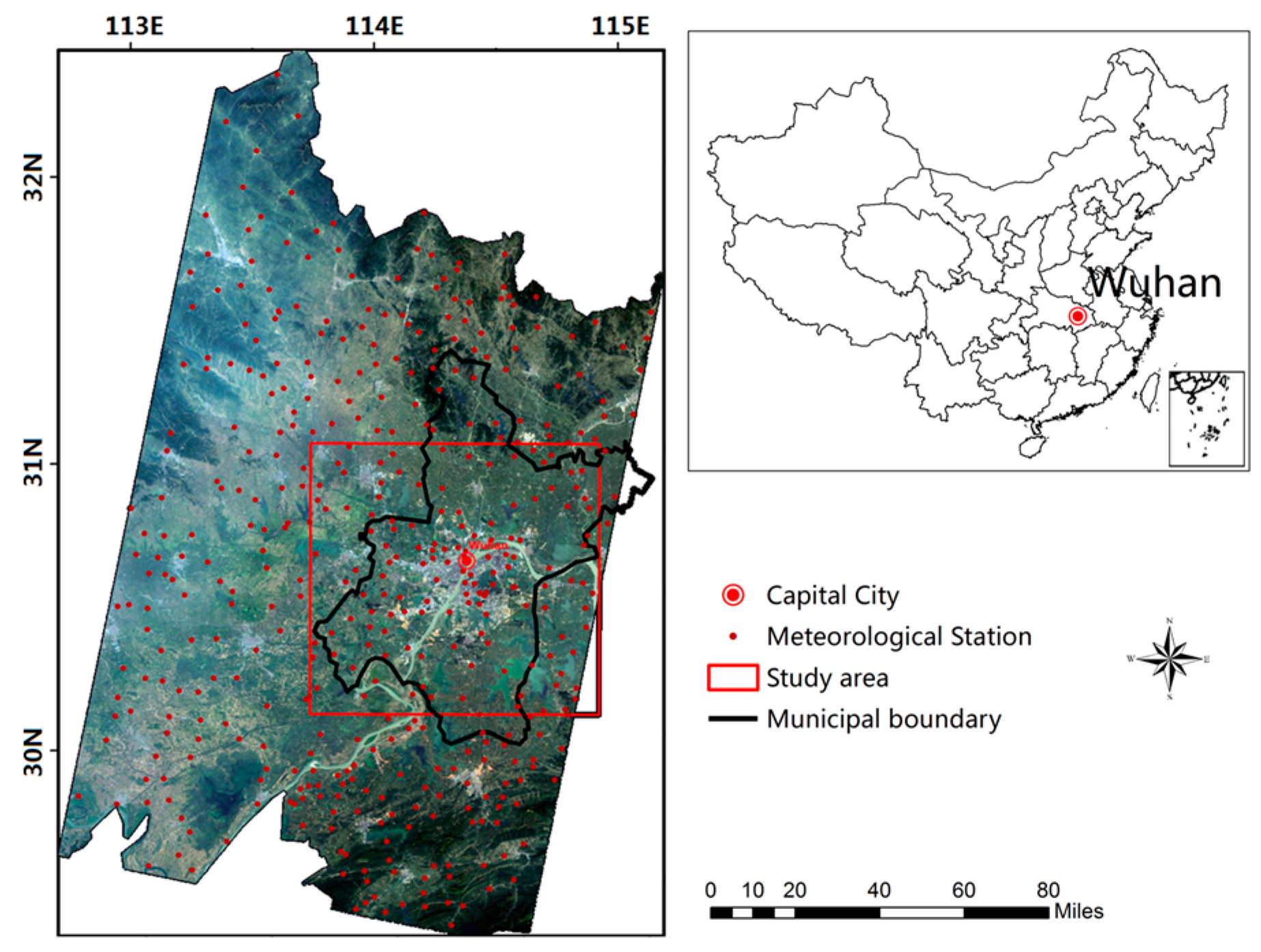
Figure 2.
Flowchart showing the methodology implemented in this study.
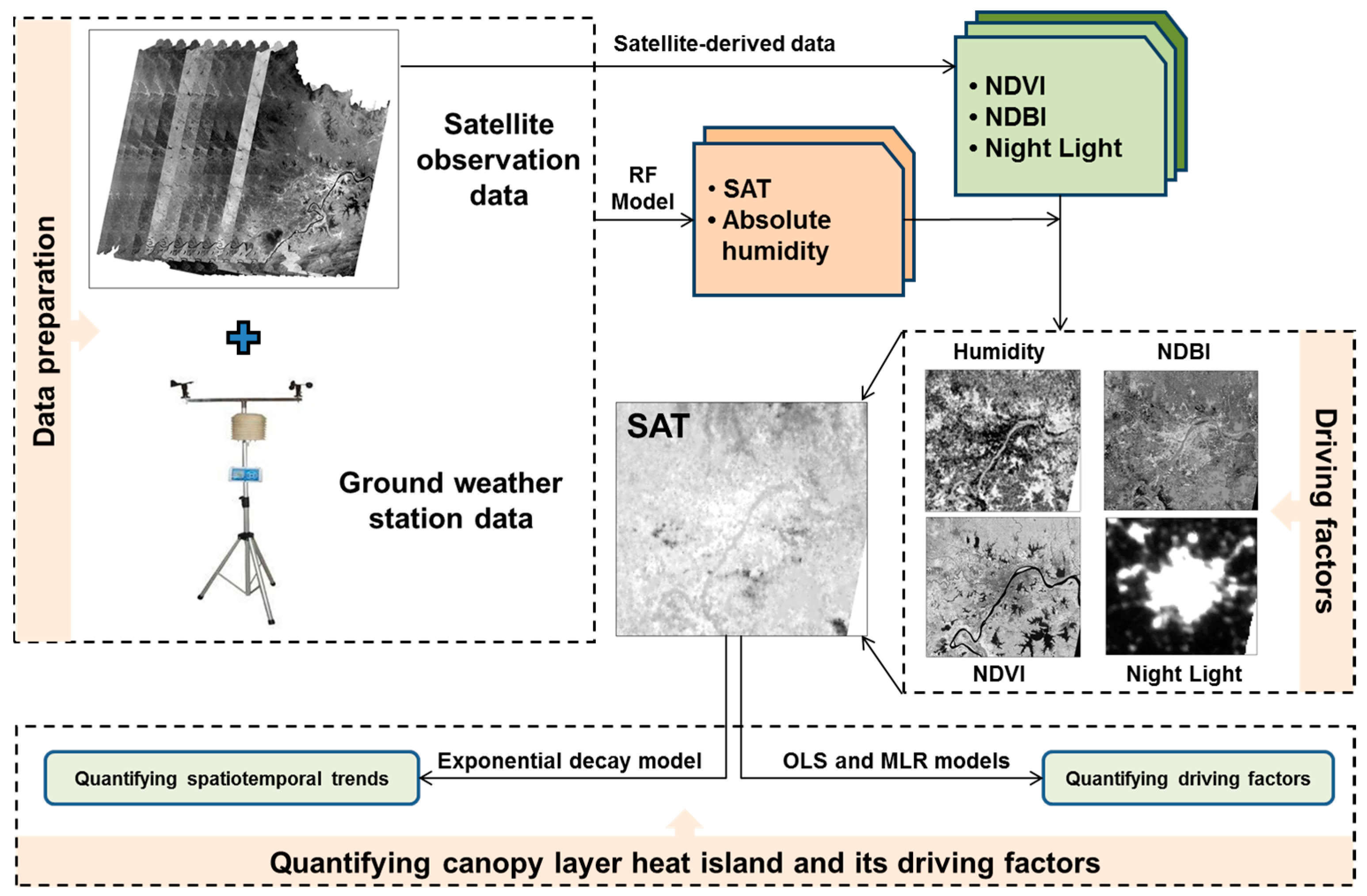
Figure 3.
Delineation of the Wuhan metropolitan area and nine buffer zones (a). Daily mean SAT in summer (b). Daily mean SAT in winter (c). The red border represents the manually delineated urban area, and the white borders are nine buffer zones that each cover the same area of land as the urban area.
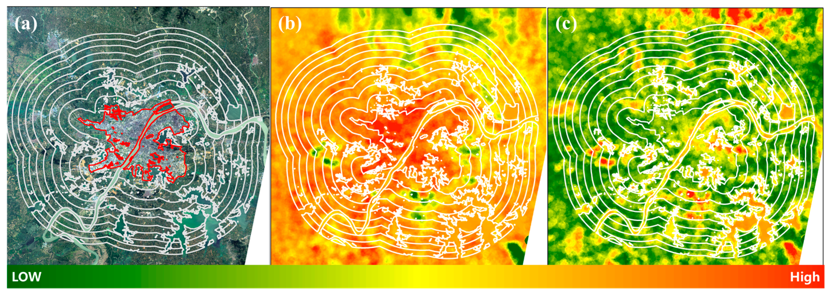
Figure 4.
Scatter plot of the observed versus predicted SAT values obtained using the random forest model. No correction (black); Correction (red) based on the regression calibration approach.
Figure 4.
Scatter plot of the observed versus predicted SAT values obtained using the random forest model. No correction (black); Correction (red) based on the regression calibration approach.

Figure 5.
The prediction errors (RMSE) of SAT at an interval of 1 h obtained using the random forest model. Correction in summer = “C in S”; correction in winter = “C in W”; non-correction in summer = “NC in S”; non-correction in winter = “NC in W”. “Correction” indicates that the predicted values estimated from the random forest model were stretched based on the regression calibration approach. “Non-correction” represents the predicted values based on the random forest model.
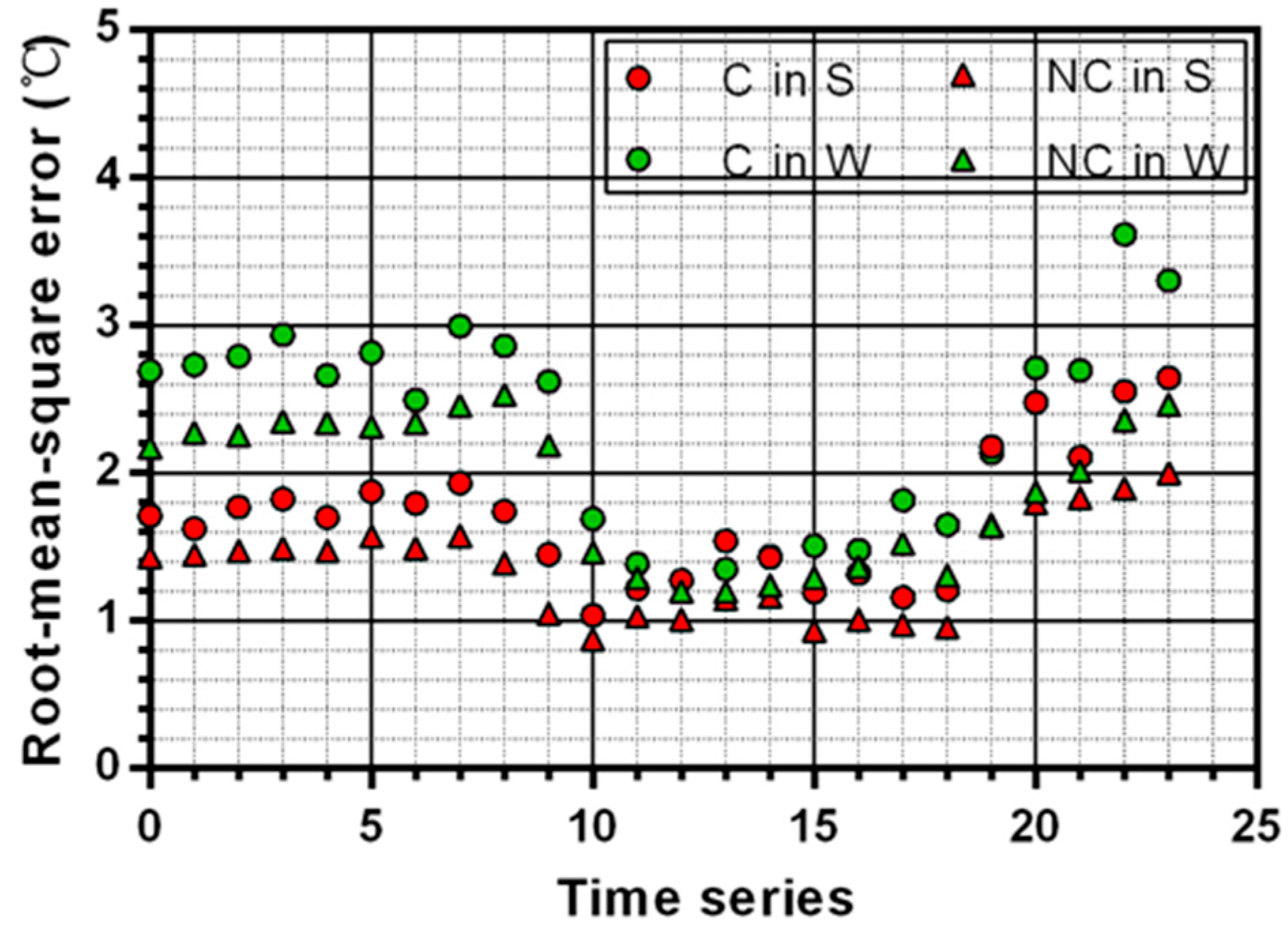
Figure 6.
Land-cover maps obtained from Landsat-8 data for the city of Wuhan, China, and building/road and woodland/grassland derived from ZY-3 satellite data (with a spatial resolution of 2.5 m) for the Wuhan metropolitan area.
Figure 6.
Land-cover maps obtained from Landsat-8 data for the city of Wuhan, China, and building/road and woodland/grassland derived from ZY-3 satellite data (with a spatial resolution of 2.5 m) for the Wuhan metropolitan area.

Figure 7.
Daily mean SAT in (a) summer and (b) winter.
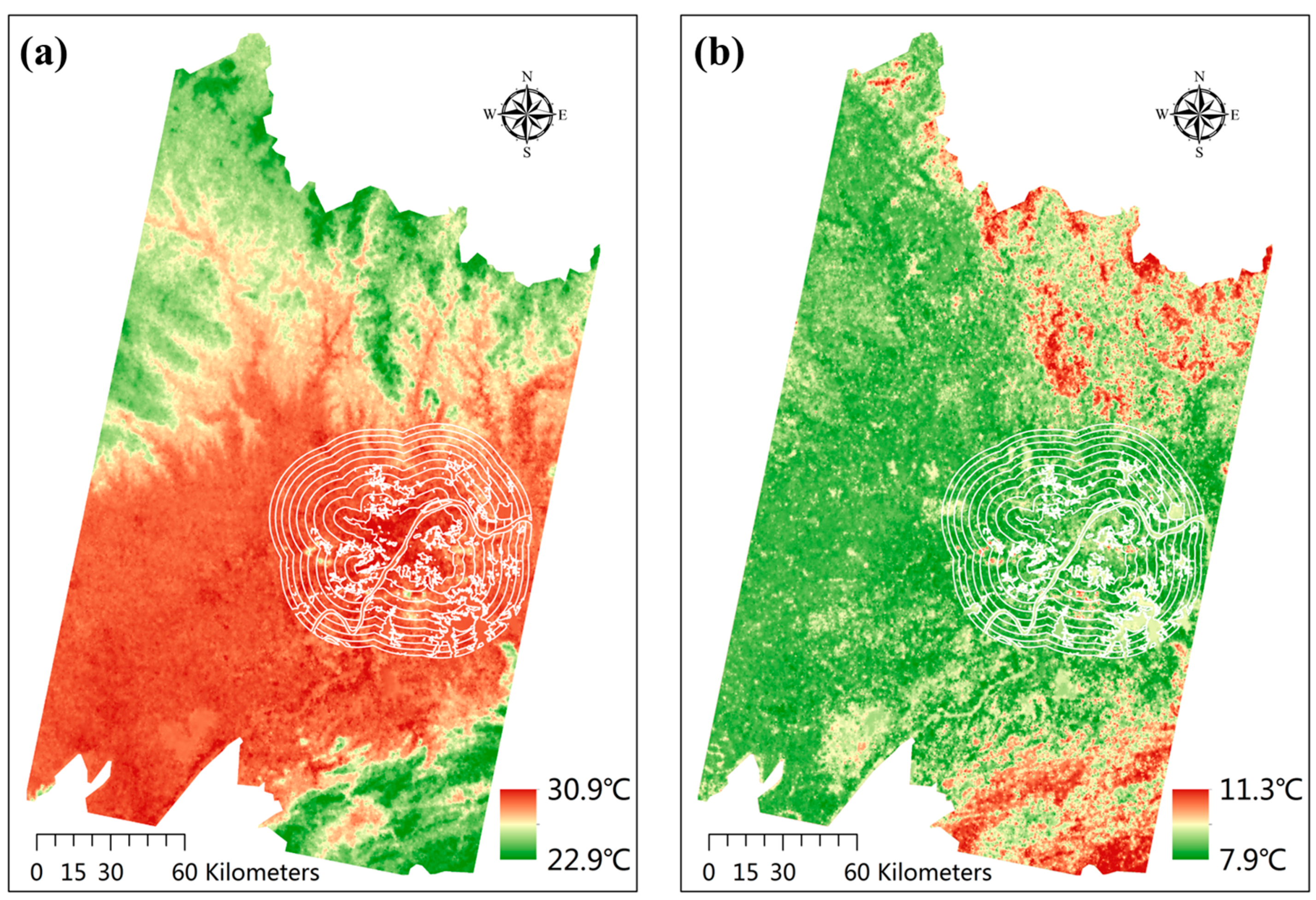
Figure 8.
LSTs derived from Landsat-8 and MODIS-terra.
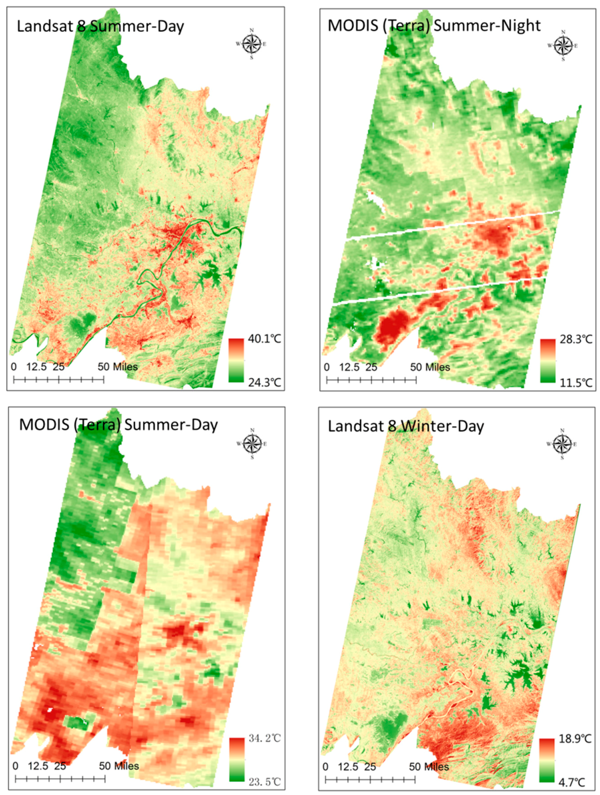
Figure 9.
Exponential decay trends of (a) the daily mean CLHII and (b) the SUHII along the urban-rural (buffer zones 0–9) gradients in summer and winter. The LST products, as shown in Figure 8, were derived from MODIS-Terra (MOD11A1) and Landsat-8 imageries. The hollow black circles indicate missing data caused by cloud or mist disturbance; 0 represents the metropolitan area, and 1–9 represents the distance of buffer zone to the boundary of metropolitan area (1–3.9 km, 2–8.1 km, 3–12 km, 4–15.5 km, 5–19 km, 6–22 km, 7–25 km, 8–27.6 km, 9–30 km).
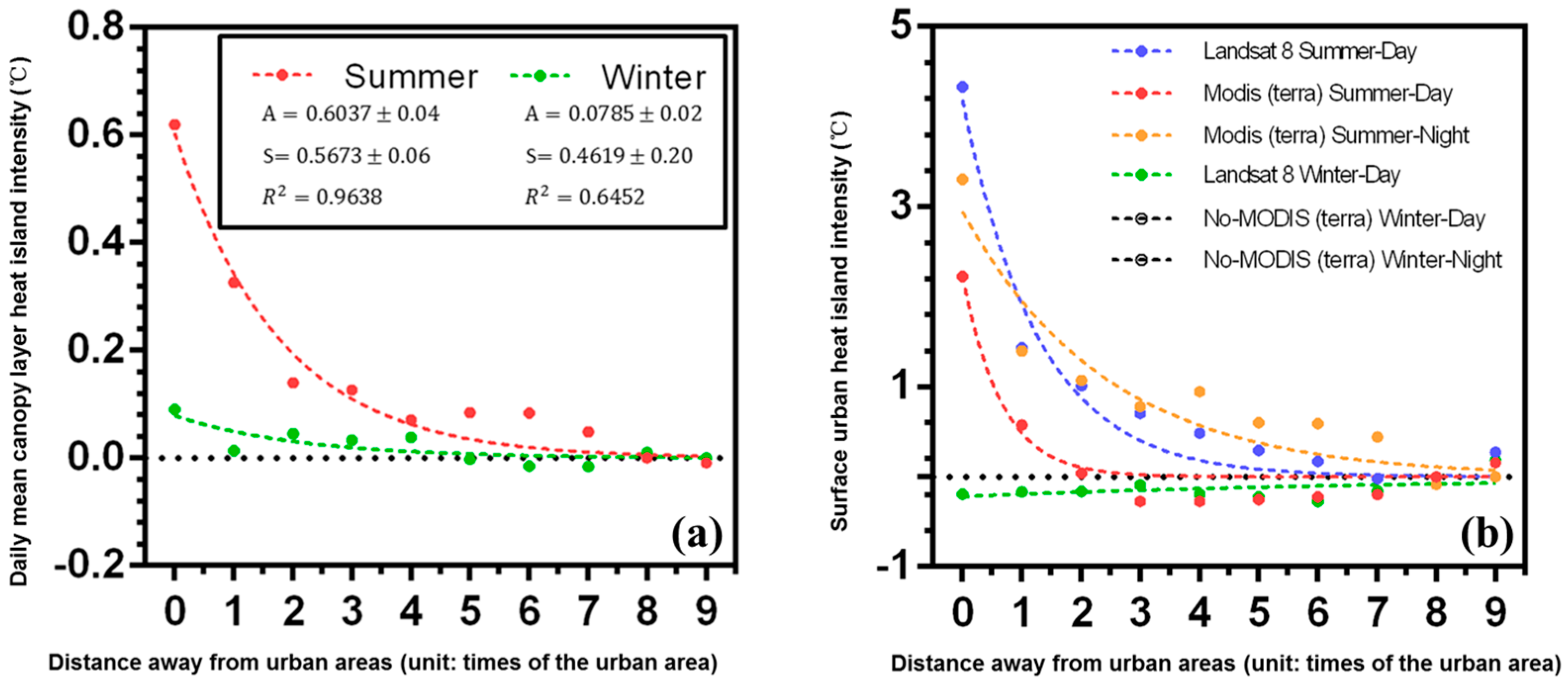
Figure 10.
Exponential decay trends of the CLHI along the urban-rural (buffer zones 0–9) gradients at an interval of 2 h in summer and winter; 0 represents the metropolitan area, and 1–9 represents the distance of buffer zone to the boundary of metropolitan area (1–3.9 km, 2–8.1 km, 3–12 km, 4–15.5 km, 5–19 km, 6–22 km, 7–25 km, 8–27.6 km, 9–30 km).

Figure 11.
The change trends of daily SAT (maximum, mean, and minimum value) obtained the using the random forest model and regression calibration approach, and observed daily mean values (black line) for the Wuhan metropolitan area: (a) SAT in summer; and (b) SAT in winter. The red shading and green shading depict the mean ± one standard deviation of the SAT in summer and winter, respectively.

Figure 12.
The spatiotemporal trends of the CLHI, including (a) the CLHII; and (b) the CLHI footprint for 17 September 2013 (summer), and 23 January 2014 (winter), in the Wuhan metropolitan area. The circumference represents the time series range from 0:00 to 23:00; the distance away from the center represents the CLHI footprint.

Figure 13.
Single-level relationships between daily mean CLHII and its driving factors quantified by the OLS model. The red lines represent summer; the green lines represent winter.
Figure 13.
Single-level relationships between daily mean CLHII and its driving factors quantified by the OLS model. The red lines represent summer; the green lines represent winter.
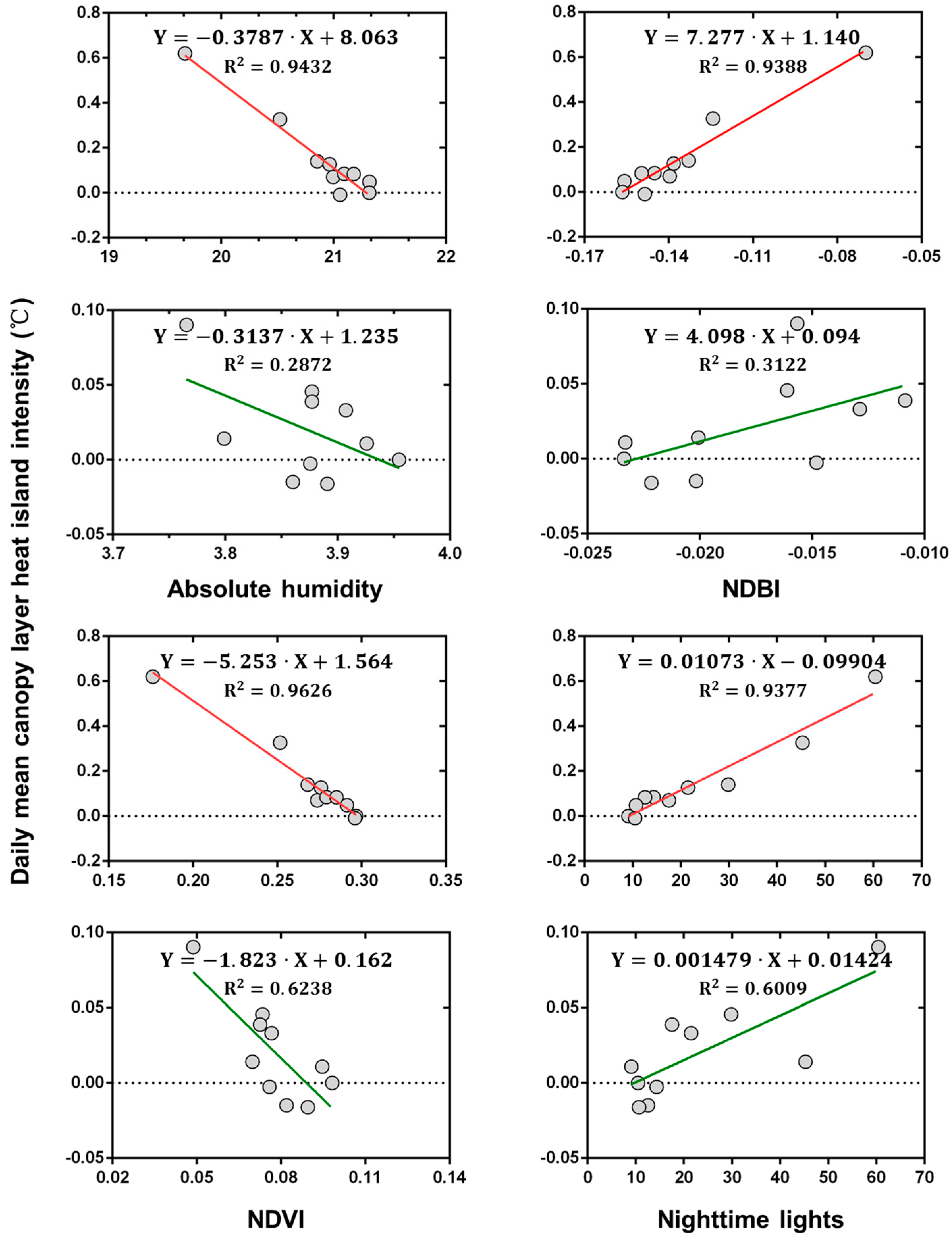
Figure 14.
Buffer residuals along the urban-rural (buffer zones 0–9) gradients based on the MLR model in (a) summer and (b) winter. Alpha = 0.1 (90% confidence interval).
Figure 14.
Buffer residuals along the urban-rural (buffer zones 0–9) gradients based on the MLR model in (a) summer and (b) winter. Alpha = 0.1 (90% confidence interval).

Table 1.
The mean values of the normalized difference built-up index (NDBI), the normalized difference vegetation index (NDVI), and absolute humidity for the different land-cover types in summer and winter.
Table 1.
The mean values of the normalized difference built-up index (NDBI), the normalized difference vegetation index (NDVI), and absolute humidity for the different land-cover types in summer and winter.
| Metric | NDBI | NDVI | Absolute Humidity (g/m3) | |||
|---|---|---|---|---|---|---|
| Summer | Winter | Summer | Winter | Summer | Winter | |
| Building | −0.04 | −0.02 | 0.13 | 0.03 | 17.25 | 3.75 |
| Road | −0.05 | −0.01 | 0.13 | 0.03 | 17.25 | 3.75 |
| Woodland | −0.14 | −0.05 | 0.26 | 0.08 | 21.34 | 4.09 |
| Herbage | −0.16 | −0.02 | 0.31 | 0.07 | 20.84 | 3.79 |
Table 2.
MLR model: estimated correlation coefficients and interval between daily mean CLHII and its metrics in summer and winter. Summer: p < 0.01, R2 = 0.99; winter: p = 0.01064, R2 = 0.89; alpha = 0.1 (90% confidence interval).
Table 2.
MLR model: estimated correlation coefficients and interval between daily mean CLHII and its metrics in summer and winter. Summer: p < 0.01, R2 = 0.99; winter: p = 0.01064, R2 = 0.89; alpha = 0.1 (90% confidence interval).
| Metric | Constant | Absolute Humidity | |||
| Summer | Winter | Summer | Winter | ||
| Coefficients | 6.19 | −3.21 | −0.26 | 0.90 | |
| Confidence Interval (90%) | [−2.75, 15.13] | [−5.55, −0.87] | [−0.71, 0.19] | [0.23, 1.57] | |
| NDBI | NDVI | DN of Nighttime Lights | |||
| Summer | Winter | Summer | Winter | Summer | Winter |
| −10.83 | 3.04 | −8.13 | −4.56 | 0.003 | 0.001 |
| [−22.98, 1.32] | [−10.06, 3.98] | [−13.26, −3.00] | [−9.67, 0.55] | [−0.001, 0.007] | [−0.001, 0.003] |
Table 3.
Comparison between SUHII and CLHII (~represents NULL).
| Summer (17 September 2013) | Winter (23 January 2014) | ||||
|---|---|---|---|---|---|
| Event | Time | Magnitude | Event | Time | Magnitude |
| Maximum CLCI effect | 7:00 | −0.39 °C | Maximum CLCI effect | 1:00 | −0.95 °C |
| Lowest SAT | 7:00 | 24.88 °C | Maximum CLHI effect | 5:00 | 1.15 °C |
| Maximum CLHI effect | 14:00 | 1.42 °C | Lowest SAT | 6:00 | −4.52 °C |
| Mean SAT | 14:00 | 35.69 °C | Highest mean SAT | 16:00 | 20.84 °C |
| Highest SAT | 15:00 | 42.27 °C | Highest SAT | 16:00 | 22.77 °C |
| MODIS-SUHI | 10:30 | 3.3 °C | ~ | ~ | ~ |
| Landsat 8-SUHI | 10:58 | 4.3 °C | Landsat 8-SUHI | 10:58 | −0.19 °C |
| MODIS-SUHI | 22:30 | 2.2 °C | ~ | ~ | ~ |
© 2017 by the authors. Licensee MDPI, Basel, Switzerland. This article is an open access article distributed under the terms and conditions of the Creative Commons Attribution (CC BY) license (http://creativecommons.org/licenses/by/4.0/).
Share and Cite
MDPI and ACS Style
Li, L.; Huang, X.; Li, J.; Wen, D. Quantifying the Spatiotemporal Trends of Canopy Layer Heat Island (CLHI) and Its Driving Factors over Wuhan, China with Satellite Remote Sensing. Remote Sens. 2017, 9, 536. https://doi.org/10.3390/rs9060536
AMA Style
Li L, Huang X, Li J, Wen D. Quantifying the Spatiotemporal Trends of Canopy Layer Heat Island (CLHI) and Its Driving Factors over Wuhan, China with Satellite Remote Sensing. Remote Sensing. 2017; 9(6):536. https://doi.org/10.3390/rs9060536
Chicago/Turabian StyleLi, Long, Xin Huang, Jiayi Li, and Dawei Wen. 2017. "Quantifying the Spatiotemporal Trends of Canopy Layer Heat Island (CLHI) and Its Driving Factors over Wuhan, China with Satellite Remote Sensing" Remote Sensing 9, no. 6: 536. https://doi.org/10.3390/rs9060536
Note that from the first issue of 2016, this journal uses article numbers instead of page numbers. See further details here.