
Urbanization Effects on Vegetation and Surface Urban Heat Islands in China’s Yangtze River Basin


1
Laboratory of Critical Zone Evolution, School of Earth Sciences, China University of Geosciences, Wuhan 430074, China
2
School of Remote Sensing and Information Engineering, Wuhan University, Wuhan 430079, China
3
State Key Laboratory of Information Engineering in Surveying, Mapping and Remote Sensing, Wuhan University, Wuhan 430079, China
*
Authors to whom correspondence should be addressed.
Remote Sens. 2017, 9(6), 540; https://doi.org/10.3390/rs9060540
Submission received: 12 April 2017
/
Revised: 12 May 2017
/
Accepted: 29 May 2017
/
Published: 30 May 2017
Abstract
:In the context of rapid urbanization, systematic research about temporal trends of urbanization effects (UEs) on urban environment is needed. In this study, MODIS (Moderate Resolution Imaging Spectroradiometer) land surface temperature (LST) data and enhanced vegetation index (EVI) data were used to analyze the temporal trends of UEs on vegetation and surface urban heat islands (SUHIs) at 10 big cities in Yangtze River Basin (YRB), China during 2001–2016. The urban and rural areas in each city were derived from MODIS land cover data and nighttime light data. It was found that the UEs on vegetation and SUHIs were increasingly significant in YRB, China. The ∆EVI (the UEs on vegetation, urban EVI minus rural EVI) decreased significantly (p < 0.05) in 9, 7 and 5 out of 10 cities for annual, summer and winter, respectively. The annual daytime and nighttime SUHI intensity (SUHII; urban LST minus rural LST) increased significantly (p < 0.05) in 10 and 4 out of 10 cities, respectively. The increasing rate of daytime SUHII and the decreasing rate of ∆EVI in old urban areas were much less than the whole urban area (0.034 °C/year vs. 0.077 °C/year for annual daytime SUHII; 0.00209/year vs. 0.00329/year for ∆EVI). The correlation analyses indicated that the annual and summer daytime SUHII were significantly negatively correlated with ∆EVI in most cities. The decreasing ∆EVI may also contribute to the increasing nighttime SUHII. In addition, the significant negative correlations (r < −0.5, p < 0.1) between inter-annual linear slope of ∆EVI and SUHII were observed, which suggested that the cities with higher decreasing rates of ∆EVI may show higher increasing rates of SUHII.

1. Introduction
Urbanization, the process of the agricultural-based rural society transforming to the industrial-based urban society, is becoming an increasingly serious problem. The urban population around the world has doubled from 1750 million in 1980 to 3571 million in 2010, and this number will reach up to 5058 million in 2030 [1]. In addition, the increasing rate of global urban area is twice as fast as population growth [2]. Rapid urbanization can bring a series of problems, including urban heat island [3], reduction of cropland and vegetation coverage [4], changes of land surface phenology [5], and air pollution [6]. Thus, the magnitudes, the temporal trends and the relationships between the above-mentioned problems due to urbanization should be comprehensively investigated.
One of the serious problems due to urbanization is the reduction of vegetation coverage. Vegetation plays very important roles in terrestrial ecosystems and can bring a lot of benefits to human society [7]. The forest is even likened to the lungs of the earth. Vegetation can mitigate the air pollution [8], noise pollution [9] and urban heat island [10]; it can also prevent the loss of soil and water through retention of precipitation [11], and alleviate the greenhouse effect through absorbing CO2 [12]. However, a series of benefits from vegetation will also be lost due to urbanization; for example, urbanization can transform the forest and cropland to built-up land, reducing the vegetation coverage directly.
Urban heat island (UHI), a problem due to urbanization, refers to the phenomenon where the air temperature in the city is higher than that of the countryside, which has a large amount of negative effects [3]. It can influence vegetation activity [5] and climate [13]. In addition, UHI can affect human health [14] and energy consumption [15,16]. The UHI may lead to more serious problems in the context of global warming [17]; for example, Goggins et al. [18] indicated when the air temperature increased 1 °C (above 29 °C), mortality can increase 4.1% accordingly.
Remote sensing provided a new method for studying the earth surface process, including urbanization [19], hydrology [20], agriculture [21], UHI [3] and disaster monitoring [22]. The urbanization effects (UEs) on vegetation have been investigated in many studies; for example, Zhou et al. [7] used the MODIS enhanced vegetation index (EVI) data to study the UEs on vegetation. The results indicated that the EVI decreased significantly with increasing urban development intensity for most cities in China. Liu et al. [23] used normalized difference vegetation index (NDVI) to analyze the UEs on vegetation for 50 cities in the world during 1981–2010, which indicated that urbanization did not necessarily lead to decreasing vegetation (NDVI), but decreasing ∆NDVI between urban and rural areas was observed. The temperature monitored by remote sensing was land surface temperature (LST), which was different from the air temperature monitored by the weather stations. Therefore, the UHI monitored by remote sensing was surface UHI (SUHI). Peng et al. [10] used MODIS LST data to study the SUHI intensity (SUHII) at 419 global big cities during 2003–2008 and the average daytime and nighttime SUHII were 1.5 °C and 1.1 °C, respectively. Zhou et al. [3] studied the SUHII at 32 major Chinese cities and the SUHII varied greatly by season, location and background climates. Alves [24] indicated that the SUHII was 12 °C in Ceres and Rialma (Brazil). However, few studies have been conducted focusing on the temporal trends of UEs on SUHII and its relationships with decreasing vegetation. Quan et al. [25] studied the relationships between temporal trends of nighttime LST and NDVI or climatic parameters in Beijing during 2000–2012 and the results showed that the temporal trend of urban nighttime LST was negatively correlated with NDVI, but an insignificant correlation was found in rural areas. Wang et al. [26] indicated that the SUHII increased significantly at outskirts of Phoenix (United States) in June during 2000–2014, which can primarily be attributed to the decreasing vegetation. Detailed study at the regional or global scale is still needed.
China has undergone fast urbanization in past decades. The proportion of urban population to total population in China was 35.9% in 2000, 55.6% in 2015, and it is predicted that this data will reach up to 68.7% in 2030 [1]. The Yangtze River Basin (YRB) plays an important role in economic development, food production and water supply in China [27,28]. For the purpose of comprehensively understanding the UEs on environment, decision-making and human beings, it is essential to systematically study the temporal trends of UEs on urban environment. Therefore, we provided a comprehensive study of UEs on vegetation and SUHII and their potential relationships.
The main purpose of this study were to: (1) reveal the 16-year averaged UEs on vegetation and SUHII in YRB, China during 2001–2016; (2) study the temporal trends of UEs on vegetation and SUHII for the whole study period; (3) examine the relationships between UEs on vegetation and SUHII. Our study can provide an important reference to study the temporal trends of UEs on the urban environment, which will be helpful for better understanding of the relationships between UEs on vegetation and SUHII.
2. Data and Methods
2.1. Study Area
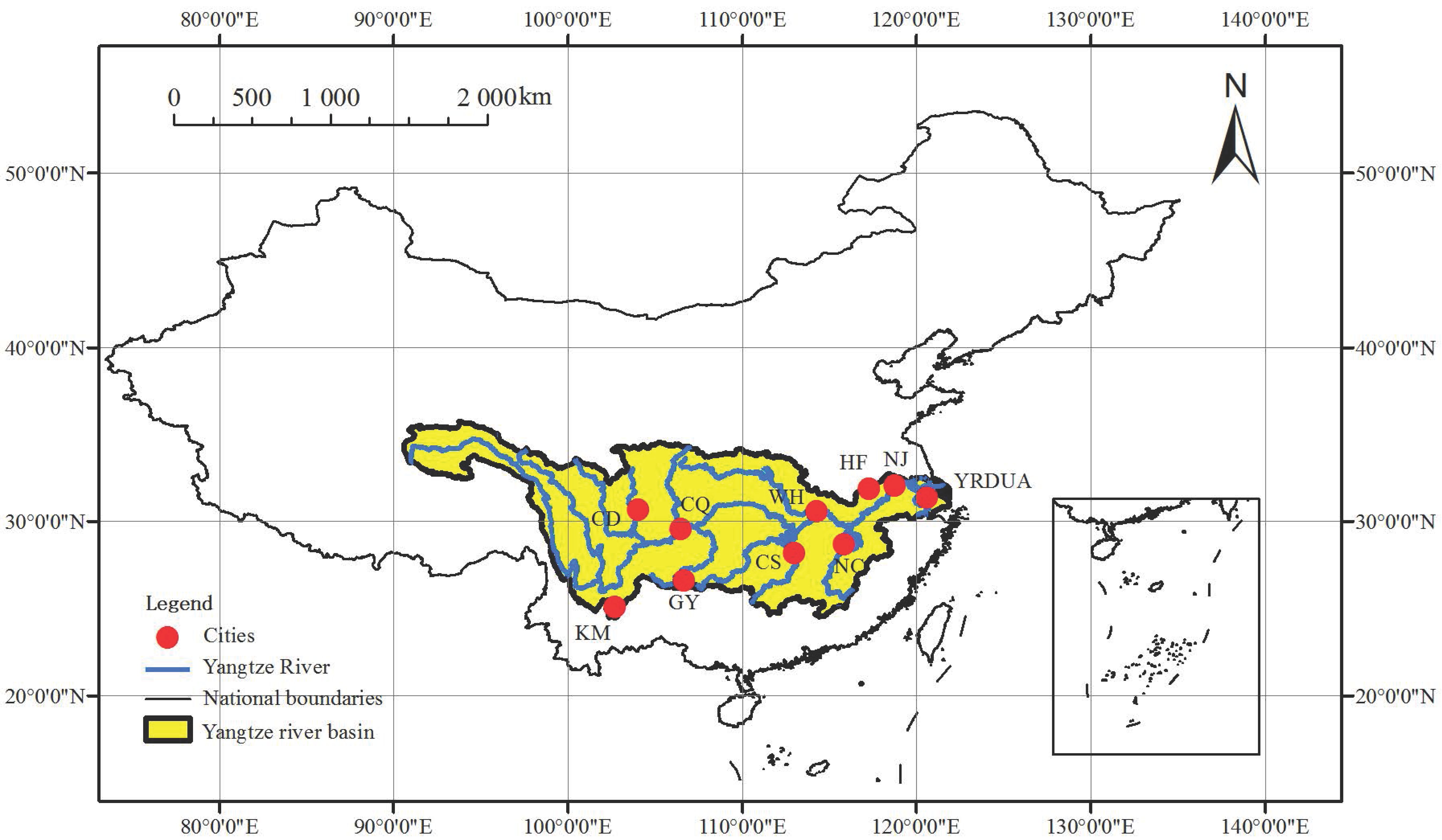
The YRB (total area: 1.8 million km2, population: 400 million) is located at the southern part of China (Figure 1). The YRB is generally characterized by a subtropical monsoon climate. The annual total precipitation in YRB is about 1070 mm, and the annual mean temperature is about 17 °C [29,30]. The Yangtze River Delta urban agglomeration (YRDUA) is one of the most famous urban agglomerations in the world [31]. In this study, YRDUA (including Shanghai, Suzhou, Changzhou and Wuxi) and another nine municipalities or provincial capitals were chosen, including Chengdu (CD), Guiyang (GY), Chongqing (CQ), Kunming (KM), Wuhan (WH), Nanchang (NC), Changsha (CS), Hefei (HF) and Nanjing (NJ) (Figure 1).
2.2. Land Cover Data
In this study, version 4 stable nighttime light data (SNLD; annual composite, 30″ spatial resolution, digital number (DN) ranging from 0 to 63) during 2001–2013 and MODIS land cover data (LCD; MCD12Q1; combined Terra and Aqua satellite; annual composite; 500 m spatial resolution (resampled to 1000 m)) during 2001–2013 were combined to generate the urban and rural areas [31,32].
2.3. MODIS LST and EVI Data
MODIS LST data has been widely used to study the SUHIs at regional scale [3,10,31,32,33,34,35,36] because of its high accuracy, wide coverage and high temporal resolution (four times pass every day; Terra satellite: 10:30 a.m. and 10:30 p.m. local time, Aqua satellite: 1:30 a.m. and 1:30 p.m. local time). In this study, the LST was derived from the MOD11A2 data (Terra satellite, 1 km spatial resolution, 8 day composite) for the period 2001–2016. The accuracy of MODIS LST product has been validated by previous studies: the errors are within ±1 K in 39 of 47 cases [37,38].
Several studies have showed that enhanced vegetation index (EVI) is more appropriate for monitoring vegetation dynamics in urban areas usually covered by sparse vegetation than the NDVI [39,40,41]. In this study, MODIS EVI data (MOD13A2, Terra satellite, 1 km spatial resolution, 16 day composite) from 2001 to 2016 was used to extract the vegetation information. In this study, the MODIS data was first reprojected and mosaicked using MODIS reprojection tool [42], and then averaged (ignoring no data value) into annual (12 months), summer (June to August) and winter (December to February) before it was processed further.
2.4. Extraction of Urban Area
The SNLD cannot be used directly because of these problems: (a) lack of calibration; (b) sensor deterioration; and (c) differences of radiometric performance [43,44,45]. Therefore, a series of calibration methods were performed (intercalibration, intra-annual composition and inter-annual calibration) according to Liu et al. [45] to solve these problems. Taiwan province was used as a reference area and the F18 2010 was used as reference data to perform the intercalibration. Detailed information about these methods can be found in Liu et al. [45]. The intercalibration equations are as follows (Equation (1)):
where B is the initial DN value of SNLD, A is the intercalibrated DN value, C1, C2, and C3 are the coefficients (Table 1).
A = C1 × B2 + C2 × B + C3
In this study, SNLD and MODIS LCD were used to generate the urban and rural areas. Both data have their advantages and disadvantages. We used the MODIS LCD to generate the urban areas in WH and there were no large variations of urban areas between 2001 and 2013 (Figure 2a,b and Figure 3a,b), which does not meet the actual characteristics of rapid urbanization in WH in past decades [46]. This suggested that the MODIS LCD is not suitable for studying the inter-annual urbanization. In addition, the SNLD was frequently used to generate the urban area across different years [44,45]. However, the SNLD data has a blooming effect; the urban area extracted from SNLD was usually larger than the real urban area [44,47]. Figure 2c and Figure 3c showed that the urban areas at WH extracted from SNLD contained the Yangtze River and some lakes, which should be removed in SUHI’s study [3,10,48]. In addition, MODIS LCD can extract the water body accurately (Figure 2d and Figure 3d). Therefore, we first used the SNLD to generate the urban areas at each city in the year 2001 and 2013, DN > 50 was used to extract the urban areas according to Liu et al. [23]. Secondly, we take the union of water body from 13 land cover maps using MODIS LCD during 2001–2013. Next, we excluded the union area of water body from urban areas derived from the SNLD, so that we can more accurately extract the urban area (Figure 2e) and cover the high temperature zone (Figure 3e). The amount of urban area in 10 cities for the year 2001 and 2013 can be found in Table 2. We further compared the urban area extracted using nighttime data with that from Landsat data (maximum likelihood classification method). The results showed that the urban area extracted using the method in this study was larger than that from Landsat data (Table 2); however, it is appropriate for this study due to these reasons: (a) the footprint of SUHI was larger than the actual urban size according to previous studies [40,48,49]; (b) the urbanization primarily occurred in the suburban areas according to previous studies [26,36]; (c) the study period in this study was 2001–2016, the land cover maps used were during 2001–2013, and the urban area may expand during 2014–2016. Finally, we generated the buffer zone between 20 and 25 km from the urban areas, and we excluded the pixel with DN > 10 (SNLD) in the 20–25 km buffer and defined it as rural area [5,41]. The rural areas in this study were set larger than previous studies, since the footprint of UEs was much larger than the urban areas in previous studies [5,40,48,49]. We did not select larger buffer zones for reducing the uncertainties due to different climate conditions and topography [48]. The accuracy of this method of defining urban area may be lower than those using the higher spatial resolution images (e.g., Landsat data), but it is fast and enough for matching the 1 km spatial resolution of MODIS EVI (MOD13A2) and LST (MOD11A2) data. Thus, this method can be applied at national, continental and global scale in future.
2.5. Calculation of UEs on Vegetation and SUHII
The SUHII was calculated using Equation (2) according to previous studies [3,10]:
where the LSTurban and LSTrural were the LST in urban and rural areas, respectively, and the ∆LST represented the SUHII. The urban and rural areas were derived from the land cover maps in the year 2013.
∆LST (SUHII) = LSTurban − LSTrural
The UEs on vegetation were calculated as (Equation (3)):
where the EVIurban and EVIrural were the EVI in urban and rural, respectively, the ∆EVI represented the UEs on vegetation.
∆EVI = EVIurban − EVIrural
In this study, we calculated the SUHII and ∆EVI during 2001–2016 using the static land cover map in the year 2013. The purpose was to compare the SUHII or ∆EVI in the same places across different years [5]. In addition, the urban area in the year 2001 was defined as old urban area (OUA), and the urbanized area (UA) was defined as the differences between the urban area in the year 2001 and 2013. Annual, summer (from June to August) and winter (from December to February) averaged SUHII and ∆EVI in each year were calculated separately. Linear regression analyses were performed in SPSS 22.0 to examine the temporal trends of UEs on vegetation (∆EVI) and SUHII in each city. The relationships between SUHII and ∆EVI were analyzed using Pearson’s correlation analysis.
3. Results
3.1. 16-Year Averaged UEs on Vegetation and SUHII
Table 3 showed the 16-year averaged UEs on vegetation in each city; all cities showed negative UEs on vegetation (∆EVI < 0), ranging from −0.157 at CQ in summer to −0.042 at YRDUA in winter. The UEs on vegetation (i.e., ∆EVI) differed greatly in each season. The variations of ∆EVI were more obvious in summer (−0.119 averaged for 10 cities), followed by annual (−0.088 averaged for 10 cities) and winter (−0.060 averaged for 10 cities).
The 16-year averaged SUHII in each city was shown in Table 4; nearly all cities showed positive SUHII (except certain cities in winter). The seasonal variations of daytime SUHII were similar to those for ∆EVI. The highest SUHII was observed on a summer day (3.07 °C averaged for 10 cities), ranging from 2.43 °C at WH to 4.49 °C at KM. In contrary, the lowest SUHII was found on a winter day (0.41 °C averaged for 10 cities), ranging from −0.46 °C at WH to 1.38 °C at KM. However, nighttime SUHII was relatively stable across seasons (0.88 °C, 1.09 °C and 0.70 °C averaged for 10 cities for annual, summer and winter, respectively), ranging from −0.07 °C at HF in winter to 2.36 °C at KM in summer.
3.2. Temporal Trends of ∆EVI in YRB during 2001–2016
Figure 4 showed the temporal trends of ∆EVI in YRB averaged for 10 cities during 2001–2016; the annual, summer and winter ∆EVI decreased significantly at the rate of −0.00329/year (p < 0.01), −0.00415/year (p < 0.01) and −0.00217/year (p < 0.01), respectively. In addition, Table 5 showed the temporal trends of ∆EVI in each city for the whole study period; the annual and summer ∆EVI decreased significantly at most cities (9 and 7 out of 10 cities for annual and summer, respectively). The most dramatic decreasing trend was observed in summer, ranging from −0.00630/year (p < 0.01) at CS to −0.00044/year (p > 0.05) at NJ. The significant decreasing trends of ∆EVI were also observed in half of the cities (5 out of 10) in winter, ranging from −0.00607/year (p < 0.01) at CD to 0.00009/year (p > 0.05) at NJ. Table 6 showed the temporal trends of ∆EVI in OUAs; although the significant decreasing trends of ∆EVI were observed in 9 out of 10 cities, the decreasing rates of ∆EVI in OUAs were much less than the whole urban areas (−0.00209/year vs. −0.00329/year averaged for 10 cities). The city showed an insignificant decreasing trend of ∆EVI at NJ, and the EVI in both OUA and rural areas showed insignificant increasing trends (0.00039/year and 0.00056/year for OUA and rural areas, respectively).
3.3. Temporal Trends of SUHII in YRB during 2001–2016
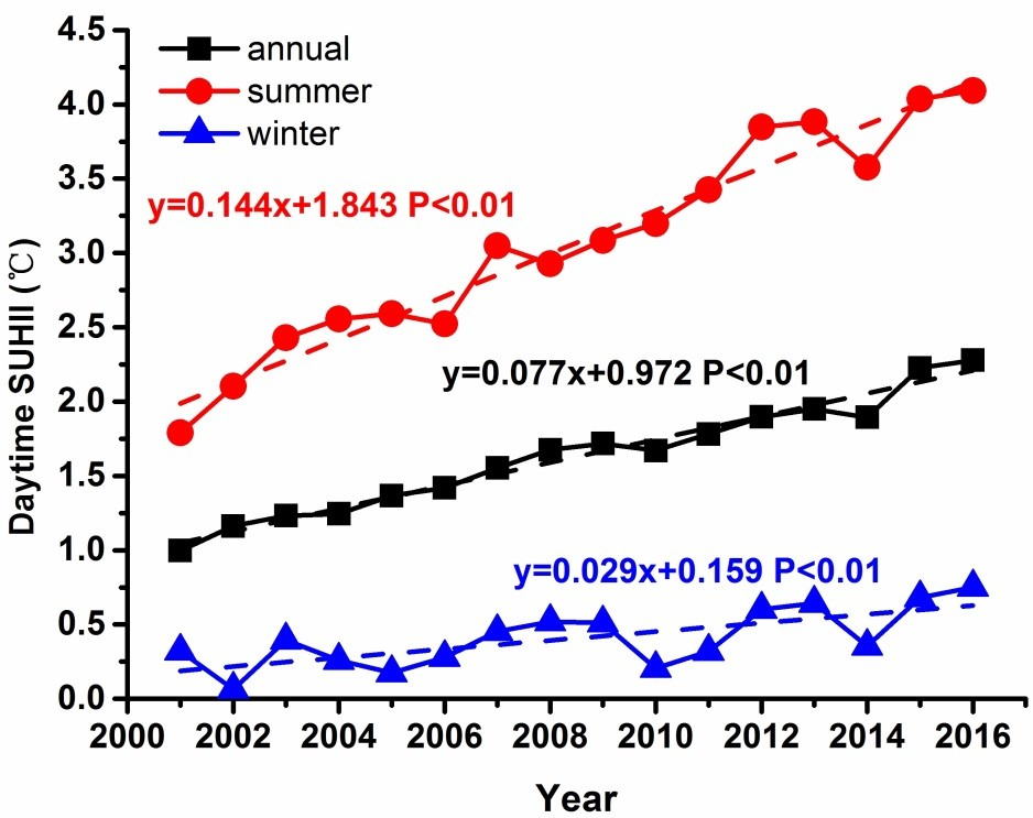
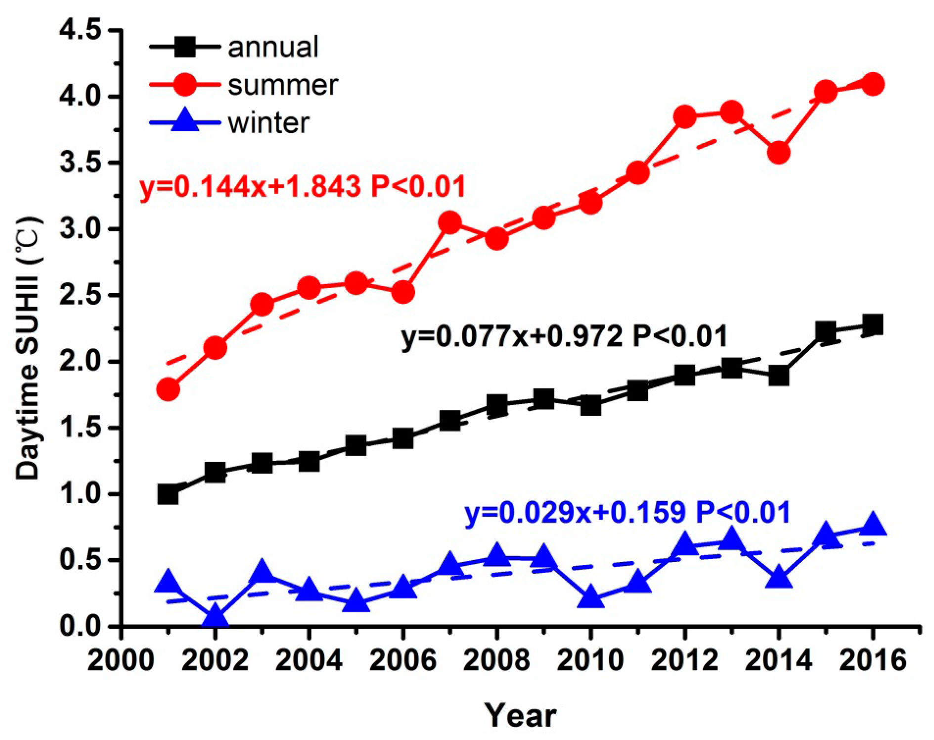
Figure 5 showed the temporal trends of daytime SUHII averaged for 10 cities during 2001–2016; the annual, summer and winter SUHII increased significantly for the whole study period. For daytime SUHII, the highest increasing rate was in summer (0.144 °C/year, p < 0.01), followed by annual SUHII (0.077 °C/year, p < 0.01) and winter SUHII (0.029 °C/year, p < 0.01). Meanwhile, the increasing rates of nighttime SUHII were similar across different seasons (Figure 6); the annual, summer and winter nighttime SUHII increased significantly at the rate of 0.023 °C/year (p < 0.01), 0.033 °C/year (p < 0.01) and 0.022 °C/year (p < 0.05), respectively.
Table 7 showed the temporal trends of SUHII in each city for the period 2001–2016; the increasing trends of SUHII were observed in all cities for annual, summer and winter scales. The annual and summer daytime SUHII increased significantly for nearly all above cities (10 and 9 out of 10 cities for annual and summer, respectively) for the whole study period. The highest increasing rates were mainly in summer, ranging from 0.037 °C/year (p > 0.05) in KM to 0.233 °C/year (p < 0.01) in CD. Meanwhile, the annual and summer nighttime SUHII increased significantly at about half of the cities (4 and 5 out of 10 cities for annual and summer, respectively). The highest increasing rates of annual and summer nighttime SUHII were observed at CQ (0.041 °C/year (p < 0.01) and 0.086 °C/year (p < 0.01) for annual and summer, respectively). In addition, the winter daytime and nighttime SUHII increased significantly only at a few cities (3 and 3 out of 10 cities for daytime and nighttime SUHII in winter, respectively). The highest increasing trends of daytime and nighttime SUHII in winter were all found at CQ (0.134 °C/year (p < 0.01) and 0.047 °C/year (p < 0.01) for daytime and nighttime SUHII in winter, respectively). The increasing rates of annual daytime SUHII in OUAs was lower than the whole urban area for all cities (0.034 °C/year vs. 0.077 °C/year, Table 6 and Table 7). However, the increasing rate of nighttime SUHII in OUAs was similar to the whole urban area (0.34 °C/year vs. 0.027 °C/year, Table 6 and Table 7).
3.4. The Relationships between SUHII and ∆EVI in YRB during 2001–2016
Table 8 showed the Pearson’s correlation coefficients between SUHII and ∆EVI at each city during 2001–2016. The negative correlations were observed for nearly all cities in annual and summer scales. The significant negative correlations between annual (or summer) daytime SUHII and ∆EVI were observed in most cities, ranging from −0.895 (p < 0.01) at CQ to −0.442 (p > 0.05) at NC for annual scale (or −0.953 (p < 0.01) at CD to −0.315 (p > 0.05) at GY in summer). Half of the cities (5 out of 10 cities) also showed significantly negative correlations between annual or summer nighttime SUHII and ∆EVI. Moreover, only 4 out of 10 cities showed significant negative correlations between SUHII and ∆EVI in winter nights (CS: −0.715 (p < 0.01); CQ: −0.621 (p < 0.05); KM: −0.749 (p < 0.01); NC: −0.612 (p < 0.05)), and the insignificant correlations were found in the remaining 6 cities.
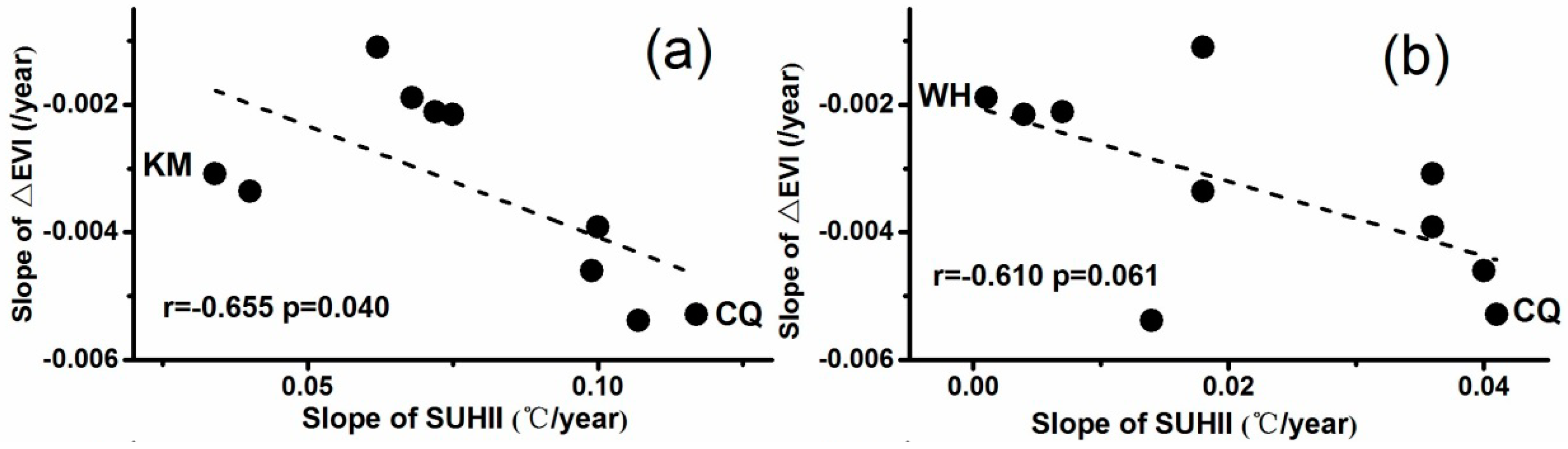
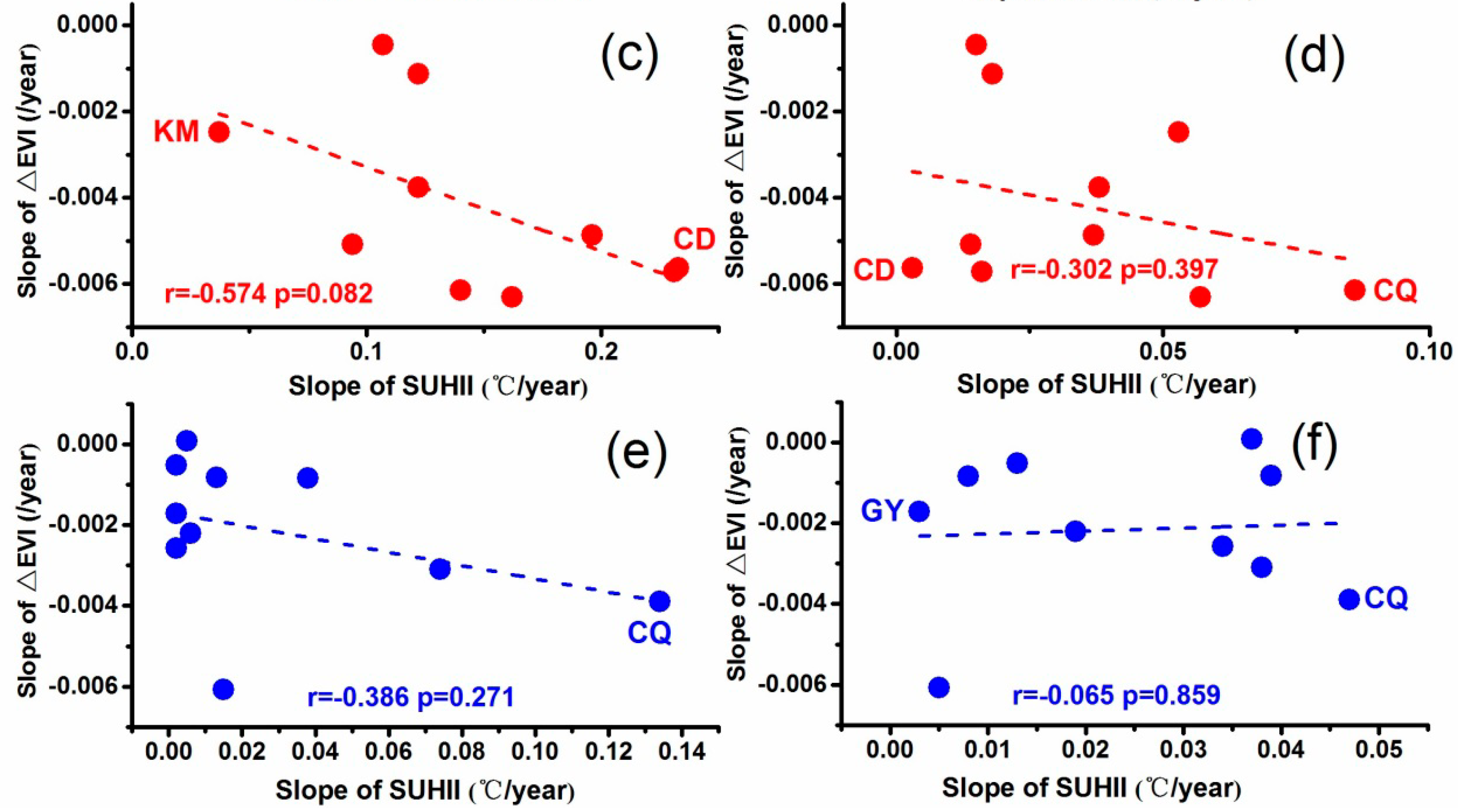
In addition, correlation analyses between linear slope of SUHII and ∆EVI were also conducted (Figure 7); all of the correlation coefficients (r) were less than −0.3 except in winter night. High negative correlations were observed in annual daytime, annual nighttime and summer daytime (r < −0.5, p < 0.1). This suggested that the higher decreasing rate of ∆EVI can lead to higher increasing rates of SUHII; for example, the second highest decreasing rate of annual ∆EVI (−0.00529/year, p < 0.01) and the highest increasing rates of annual daytime and nighttime SUHII (0.117 °C/year (p < 0.01) and 0.041 °C/year (p < 0.01) for daytime and nighttime SUHII, respectively) were all observed at CQ. The second lowest decreasing rate of ∆EVI (−0.189/year, p < 0.01) and the lowest increasing rate of nighttime SUHII (0.001 °C/year, p > 0.05) were found at WH, therefore, the relationships between ∆EVI and SUHII can be verified in both spatial and temporal scales.
4. Discussion
4.1. 16-Year Averaged UEs on Vegetation and SUHII
The ∆EVI and SUHII were averaged for the period 2001–2016. The UEs on vegetation (∆EVI) and SUHII were evident at above 10 cities in YRB, China. For all the cities averaged, the annual SUHII in daytime was higher than in nighttime (1.63 °C vs. 0.88 °C), and the SUHII in summer was higher than in winter (3.07 °C vs. 0.41 °C for daytime and 1.09 °C vs. 0.70 °C for nighttime). These results were similar to previous studies [3,10,32] and can be attributed to vegetation activities. Vegetation can release more latent heat fluxes but less sensible heat fluxes (than the artificial impervious surfaces: roads and buildings) by evapotranspiration and then decrease the temperature [3,26,35]. However, rapid urbanization transformed the cropland and forest to impervious surfaces, decreasing the vegetation coverage and increasing the SUHII. Meanwhile, the highest EVI was generally observed in summer in the Northern Hemisphere, so the UEs on vegetation (∆EVI) may be more significant in summer. For all the cities combined, the ∆EVI was lower in summer (−0.119) than in annual (−0.088) and winter (−0.060). Therefore, the higher SUHII was generally observed in summer. Moreover, vegetation evapotranspiration mostly occurred during daytime, which may lead to the higher SUHII in daytime than in nighttime [3,10,26].
4.2. Temporal Trends of UEs on Vegetation and SUHII in YRB, China
The annual ∆EVI decreased at the above cities in YRB during 2001–2016, which suggested that the UEs on vegetation are becoming increasingly serious. More people will live (and more factories will be built) in the city due to rapid urbanization; therefore, the cropland or forest will be cut down. A series of problems may arise, such as reduction of cropland production [21,50], UHI [10], air pollution [8] and so on. For the 10 cities averaged, the annual ∆EVI decreased at the rate of −0.00329/year (p < 0.01); the decreasing trend in summer (−0.00415/year, p < 0.01) was higher than in winter (−0.00217/year, p < 0.01). The growing season vegetation is mainly during April to October in the Northern Hemisphere [7], and the highest EVI may be in summer, so the decreasing vegetation was more evident in summer. Comparatively, the decreasing trends of annual ∆EVI in OUAs were much lower than the whole urban areas (−0.00209/year and −0.00329/year averaged for 10 cities for OUAs and the whole urban area, respectively), which was probably due to the Chinese governments’ policy of creating and preserving the vegetated area to deal with urbanization [41,51].
The temporal trends of SUHII at 10 cities in YRB had experienced great changes during 2001–2016. The increasing trends of SUHII were observed at the above cities in different time periods (annual daytime, annual nighttime, summer daytime, summer nighttime, winter daytime and winter nighttime; Table 7). For 10 cities combined, the annual daytime and nighttime SUHII increased significantly at the rates of 0.077 °C/year (p < 0.01) and 0.033 °C/year (p < 0.01), respectively. The decreasing vegetation may be a major factor contributing to the above results. The decreasing vegetation area due to the urbanization led to the reduction of cooling effect and finally increasing the LST in urban areas. Meanwhile, the increasing rate of daytime SUHII in summer was about twice and five times as much as annual and winter scales, respectively, which can be attributed to the different vegetation activities across different seasons. In addition, more anthropogenic heat emission and artificial impervious surfaces (roads and buildings) resulting from urbanization can also lead to the increasing SUHII [3,10]. In order to solve the increasingly serious problem of UHI, some effective measures should be adopted immediately. In addition to planting more trees, pavements and roves with high albedo and low heat storage should be applied to mitigate the UHI [52,53].
4.3. The Relationships between SUHII and ∆EVI
In this study, the correlation analyses between SUHII and ∆EVI were performed in the same city across different years, which were different from previous studies in the same year across different cities [3,10,32]. The significant negative correlations between annual and summer daytime SUHII and ∆EVI were generally observed at the above cities in YRB, China. These results were generally similar with those from Peng et al. [10] and Zhou et al. [3] (the daytime SUHII was negatively correlated with ∆EVI). However, it was found in this study that the nighttime SUHII was negatively correlated with ∆EVI in most cities (except NJ with insignificant positive correlation in summer nights), and the significant negative correlations were observed in nearly half of the cities. This was different from the insignificant correlations between SUHII and ∆EVI in previous studies [3,10]. The vegetation reducing the nighttime SUHII has been demonstrated using ground observations [53,54]. The decreasing vegetation and increasing impervious surfaces can increase heat stored during daytime. Therefore, more heat will be released from impervious surfaces during nighttime, leading to the increasing nighttime SUHII [25,55]. One unique phenomenon was that the SUHII was significantly negatively correlated with ∆EVI at 4 of 10 cities in winter nights. The reasons were not clear; maybe there is no clear relationship between them, since vegetation activity was very low on winter nights. The increasing SUHII in winter nights may be attributed to other factors such as anthropogenic heat release rather than ∆EVI.
The correlations between the linear slope of SUHII and ∆EVI were further analyzed; the cities with higher decreasing rates of ∆EVI showed larger increasing rates of SUHII; for example, CD and CQ showed the highest decreasing trends of annual ∆EVI, and the highest increasing trends of annual daytime SUHII were also observed at the above two cities. Therefore, the cities with higher increasing rates of SUHII should pay more attention to protect the terrestrial ecosystems. In this study, the continuous and rapid urbanization of the 10 cities was similar with other cities according to previous studies [56,57,58,59]. Future studies will focus on UEs on environment at regional or global scales.
5. Conclusions
In this study, the temporal trends of UEs on vegetation and SUHII were systematically analyzed at 10 big cities in YRB, China during 2001–2016. The correlation analyses were conducted between SUHII and ∆EVI at each city, and between linear slope of SUHII and ∆EVI. The 16-year averaged annual daytime and nighttime SUHII were 1.63 °C and 0.88 °C, respectively. The daytime SUHII in summer was higher than that in winter, but the converse result was observed in winter. The annual, summer and winter ∆EVI were −0.088, −0.119 and −0.060, respectively.
Rapid urbanization caused serious consequences at the 10 cities in YRB, China. The decreasing ∆EVI was observed in nearly all cities. For the 10 cities averaged, the temporal trends of ∆EVI decreased at the rate of −0.00329 (p < 0.01), −0.00415 (p < 0.01) and −0.00217 (p < 0.01) for annual, summer and winter, respectively. Over half of the cities showed significant decreasing trends of ∆EVI (9, 7 and 5 cities for annual, summer and winter, respectively). Meanwhile, for the 10 cities combined, both the annual daytime and nighttime SUHII increased significantly (0.077 °C/year, p < 0.01 and 0.033 °C/year, p < 0.01 for daytime and nighttime, respectively). Nearly all cities showed increasing SUHII trends except the winter daytime. The increasing rate of SUHII and decreasing rate of ∆EVI in old urban areas was less than the whole urban area (0.034 °C/year vs. 0.077 °C/year for annual daytime SUHII; 0.027 °C/year vs. 0.033 °C/year for annual nighttime SUHII; 0.00209/year vs. 0.00329/year for ∆EVI).
The negative correlations between SUHII and ∆EVI were observed in nearly all cities in annual and summer scales. The decreasing vegetation can increase the SUHII during daytime and nighttime. Meanwhile, the negative correlations between linear variation rates of SUHII and ∆EVI were observed, which suggested that the cities with higher decreasing rates of ∆EVI might have higher increasing rates of SUHII. Further studies will be conducted focusing on long-term UEs on land surface ecosystem and SUHI in regional and global scales. Other factors (e.g., anthropogenic heat release, albedo and climate factors) related to SUHI should also be investigated in future.
Acknowledgments
This work was financially supported by the National Natural Science Foundation of China (No. 41601044), the Special Fund for Basic Scientific Research of Central Colleges, China University of Geosciences, Wuhan (No. CUG15063 and CUGL170401), and the Natural Science Foundation for Distinguished Young Scholars of Hubei Province of China (No. 2016CFA051).
Author Contributions
Rui Yao and Lunche Wang designed the research; Rui Yao, Xuan Gui, Haoming Zhang and Yukun Zheng performed the experiments and analyzed the data; Rui Yao wrote the manuscript; Lunche Wang and Xin Huang revised the manuscript.
Conflicts of Interest
The authors declare no conflict of interest.
References
- United Nation Population Division. Available online: https://esa.un.org/unpd/wup/DataQuery/ (accessed on 2 April 2017).
- Angel, S.; Parent, J.; Civco, D.L.; Blei, A.; Potere, D. The dimensions of global urban expansion: Estimates and projections for all countries, 2000–2050. Prog. Plann. 2011, 75, 53–107. [Google Scholar] [CrossRef]
- Zhou, D.; Zhao, S.; Liu, S.; Zhang, L.; Zhu, C. Surface urban heat island in China's 32 major cities: Spatial patterns and drivers. Remote Sens. Environ. 2014, 152, 51–61. [Google Scholar] [CrossRef]
- Bren d'Amour, C.; Reitsma, F.; Baiocchi, G.; Barthel, S.; Guneralp, B.; Erb, K.H.; Haberl, H.; Creutzig, F.; Seto, K.C. Future urban land expansion and implications for global croplands. Proc. Natl. Acad. Sci. USA 2016. [Google Scholar] [CrossRef] [PubMed]
- Yao, R.; Wang, L.; Huang, X.; Guo, X.; Niu, Z.; Liu, H. Investigation of Urbanization Effects on Land Surface Phenology in Northeast China during 2001–2015. Remote. Sens. 2017, 9. [Google Scholar] [CrossRef]
- Tao, M.; Chen, L.; Wang, Z.; Wang, J.; Tao, J.; Wang, X. Did the widespread haze pollution over China increase during the last decade? A satellite view from space. Environ. Res. Lett. 2016, 11. [Google Scholar] [CrossRef]
- Zhou, D.; Zhao, S.; Liu, S.; Zhang, L. Spatiotemporal trends of terrestrial vegetation activity along the urban development intensity gradient in China's 32 major cities. Sci. Total Environ. 2014, 488, 136–145. [Google Scholar] [CrossRef] [PubMed]
- Nowak, D.J.; Crane, D.E.; Stevens, J.C. Air pollution removal by urban trees and shrubs in the United States. Urban For Urban Gree. 2006, 4, 115–123. [Google Scholar] [CrossRef]
- Pathak, V.; Tripathi, B.D.; Mishra, V.K. Dynamics of traffic noise in a tropical city Varanasi and its abatement through vegetation. Environ. Monit. Assess. 2007, 146, 67–75. [Google Scholar] [CrossRef] [PubMed]
- Peng, S.; Piao, S.; Ciais, P.; Friedlingstein, P.; Ottle, C.; Breon, F.M.; Nan, H.; Zhou, L.; Myneni, R.B. Surface urban heat island across 419 global big cities. Environ. Sci. Technol. 2012, 46, 696–703. [Google Scholar] [CrossRef] [PubMed]
- Oldfield, E.E.; Warren, R.J.; Felson, A.J.; Bradford, M.A.; Bugmann, H. Challenges and future directions in urban afforestation. J. Appl. Ecol. 2013, 50, 1169–1177. [Google Scholar] [CrossRef]
- Myeong, S.; Nowak, D.J.; Duggin, M.J. A temporal analysis of urban forest carbon storage using remote sensing. Remote Sens. Environ. 2006, 101, 277–282. [Google Scholar] [CrossRef]
- Arnfield, A.J. Two decades of urban climate research: A review of turbulence, exchanges of energy and water, and the urban heat island. Inter. J. Climatol. 2003, 23, 1–26. [Google Scholar] [CrossRef]
- Gong, P.; Liang, S.; Carlton, E.J.; Jiang, Q.; Wu, J.; Wang, L.; Remais, J.V. Urbanisation and health in China. Lancet 2012, 379, 843–852. [Google Scholar] [CrossRef]
- Akbari, H.; Cartalis, C.; Kolokotsa, D.; Muscio, A.; Pisello, A.L.; Rossi, F.; Santamouris, M.; Synnefa, A.; Wong, N.H.; Zinzi, M. Local climate change and urban heat island mitigation techniques—The state of the art. J. Civ. Eng. Manag. 2015, 22, 1–16. [Google Scholar] [CrossRef]
- Santamouris, M.; Cartalis, C.; Synnefa, A.; Kolokotsa, D. On the impact of urban heat island and global warming on the power demand and electricity consumption of buildings—A review. Energy Build. 2015, 98, 119–124. [Google Scholar] [CrossRef]
- Patz, J.A.; Campbell-Lendrum, D.; Holloway, T.; Foley, J.A. Impact of regional climate change on human health. Nature 2005, 438, 310–317. [Google Scholar] [CrossRef] [PubMed]
- Goggins, W.B.; Chan, E.Y.; Ng, E.; Ren, C.; Chen, L. Effect modification of the association between short-term meteorological factors and mortality by urban heat islands in Hong Kong. PLoS ONE 2012, 7. [Google Scholar] [CrossRef] [PubMed]
- Kuang, W.; Liu, J.; Dong, J.; Chi, W.; Zhang, C. The rapid and massive urban and industrial land expansions in China between 1990 and 2010: A CLUD-based analysis of their trajectories, patterns, and drivers. Landsc. Urban Plan. 2016, 145, 21–33. [Google Scholar] [CrossRef]
- Lopez-Moreno, J.I.; Valero-Garces, B.; Mark, B.; Condom, T.; Revuelto, J.; Azorin-Molina, C.; Bazo, J.; Frugone, M.; Vicente-Serrano, S.M.; Alejo-Cochachin, J. Hydrological and depositional processes associated with recent glacier recession in Yanamarey catchment, Cordillera Blanca (Peru). Sci. Total Environ. 2017, 579, 272–282. [Google Scholar] [CrossRef] [PubMed]
- He, C.; Liu, Z.; Xu, M.; Ma, Q.; Dou, Y. Urban expansion brought stress to food security in China: Evidence from decreased cropland net primary productivity. Sci. Total Environ. 2017, 576, 660–670. [Google Scholar] [CrossRef] [PubMed]
- Zormand, S.; Jafari, R.; Koupaei, S.S. Assessment of PDI, MPDI and TVDI drought indices derived from MODIS Aqua/Terra Level 1B data in natural lands. Nat. Hazards. 2016, 86, 757–777. [Google Scholar] [CrossRef]
- Liu, Y.; Wang, Y.; Peng, J.; Du, Y.; Liu, X.; Li, S.; Zhang, D. Correlations between Urbanization and Vegetation Degradation across the World’s Metropolises Using DMSP/OLS Nighttime Light Data. Remote Sens. 2015, 7, 2067–2088. [Google Scholar] [CrossRef]
- Alves, E. Seasonal and Spatial Variation of Surface Urban Heat Island Intensity in a Small Urban Agglomerate in Brazil. Climate 2016, 4. [Google Scholar] [CrossRef]
- Quan, J.; Zhan, W.; Chen, Y.; Wang, M.; Wang, J. Time series decomposition of remotely sensed land surface temperature and investigation of trends and seasonal variations in surface urban heat islands. J. Geophys. Res. Atmos. 2016, 121, 2638–2657. [Google Scholar] [CrossRef]
- Wang, C.; Myint, S.; Wang, Z.; Song, J. Spatio-Temporal Modeling of the Urban Heat Island in the Phoenix Metropolitan Area: Land Use Change Implications. Remote Sens. 2016, 8. [Google Scholar] [CrossRef]
- Gao, T.; Xie, L. Spatiotemporal changes in precipitation extremes over Yangtze River basin, China, considering the rainfall shift in the late 1970s. Glob. Planet Change 2016, 147, 106–124. [Google Scholar] [CrossRef]
- Yan, T.; Wang, J.; Huang, J. Urbanization, agricultural water use, and regional and national crop production in China. Ecol. Modell. 2015, 318, 226–235. [Google Scholar] [CrossRef]
- Xu, J.; Yang, D.; Yi, Y.; Lei, Z.; Chen, J.; Yang, W. Spatial and temporal variation of runoff in the Yangtze River basin during the past 40 years. Quat. Int. 2008, 186, 32–42. [Google Scholar] [CrossRef]
- Zhang, Q.; Xu, C.Y.; Zhang, Z.; Chen, Y.D.; Liu, C.L.; Lin, H. Spatial and temporal variability of precipitation maxima during 1960–2005 in the Yangtze River basin and possible association with large-scale circulation. J. Hydrol. 2008, 353, 215–227. [Google Scholar] [CrossRef]
- Du, H.; Wang, D.; Wang, Y.; Zhao, X.; Qin, F.; Jiang, H.; Cai, Y. Influences of land cover types, meteorological conditions, anthropogenic heat and urban area on surface urban heat island in the Yangtze River Delta Urban Agglomeration. Sci. Total Environ. 2016, 571, 461–470. [Google Scholar] [CrossRef] [PubMed]
- Wang, J.; Huang, B.; Fu, D.; Atkinson, P. Spatiotemporal Variation in Surface Urban Heat Island Intensity and Associated Determinants across Major Chinese Cities. Remote Sens. 2015, 7, 3670–3689. [Google Scholar] [CrossRef]
- Clinton, N.; Gong, P. MODIS detected surface urban heat islands and sinks: Global locations and controls. Remote Sens. Environ. 2013, 134, 294–304. [Google Scholar] [CrossRef]
- Imhoff, M.L.; Zhang, P.; Wolfe, R.E.; Bounoua, L. Remote sensing of the urban heat island effect across biomes in the continental USA. Remote Sens. Environ. 2010, 114, 504–513. [Google Scholar] [CrossRef]
- Tran, H.; Uchihama, D.; Ochi, S.; Yasuoka, Y. Assessment with satellite data of the urban heat island effects in Asian mega cities. Int. J. Appl. Earth Obs. Geoinform. 2006, 8, 34–48. [Google Scholar] [CrossRef]
- Zhou, D.; Zhang, L.; Hao, L.; Sun, G.; Liu, Y.; Zhu, C. Spatiotemporal trends of urban heat island effect along the urban development intensity gradient in China. Sci. Total Environ. 2016, 544, 617–626. [Google Scholar] [CrossRef] [PubMed]
- Rigo, G.; Parlow, E.; Oesch, D. Validation of satellite observed thermal emission with in-situ measurements over an urban surface. Remote Sens. Environ. 2006, 104, 201–210. [Google Scholar] [CrossRef]
- Wan, Z. New refinements and validation of the MODIS Land-Surface Temperature/Emissivity products. Remote Sens. Environ. 2008, 112, 59–74. [Google Scholar] [CrossRef]
- Dallimer, M.; Tang, Z.; Bibby, P.R.; Brindley, P.; Gaston, K.J.; Davies, Z.G. Temporal changes in greenspace in a highly urbanized region. Biol. Lett. 2011, 7, 763–766. [Google Scholar] [CrossRef] [PubMed]
- Zhang, X.; Friedl, M.A.; Schaaf, C.B.; Strahler, A.H.; Schneider, A. The footprint of urban climates on vegetation phenology. Geophys. Res. Lett. 2004, 31. [Google Scholar] [CrossRef]
- Zhou, D.; Zhao, S.; Zhang, L.; Liu, S. Remotely sensed assessment of urbanization effects on vegetation phenology in China's 32 major cities. Remote Sens. Environ. 2016, 176, 272–281. [Google Scholar] [CrossRef]
- MODIS Reprojection Tool V4.1 Software. Available online: https://lpdaac.usgs.gov/lpdaac/tools/modis_reprojection_tool (accessed on 31 January 2016).
- Elvidge, C.D.; Ziskin, D.; Baugh, K.E.; Tuttle, B.T.; Ghosh, T.; Pack, D.W.; Erwin, E.H.; Zhizhin, M. A Fifteen Year Record of Global Natural Gas Flaring Derived from Satellite Data. Energies 2009, 2, 595–622. [Google Scholar] [CrossRef]
- Huang, X.; Schneider, A.; Friedl, M.A. Mapping sub-pixel urban expansion in China using MODIS and DMSP/OLS nighttime lights. Remote Sens. Environ. 2016, 175, 92–108. [Google Scholar] [CrossRef]
- Liu, Z.; He, C.; Zhang, Q.; Huang, Q.; Yang, Y. Extracting the dynamics of urban expansion in China using DMSP-OLS nighttime light data from 1992 to 2008. Landsc. Urban Plan. 2012, 106, 62–72. [Google Scholar] [CrossRef]
- Shen, H.; Huang, L.; Zhang, L.; Wu, P.; Zeng, C. Long-term and fine-scale satellite monitoring of the urban heat island effect by the fusion of multi-temporal and multi-sensor remote sensed data: A 26-year case study of the city of Wuhan in China. Remote Sens. Environ. 2016, 172, 109–125. [Google Scholar] [CrossRef]
- Zhang, Q.; Seto, K. Can Night-Time Light Data Identify Typologies of Urbanization? A Global Assessment of Successes and Failures. Remote Sens. 2013, 5, 3476–3494. [Google Scholar] [CrossRef]
- Zhou, D.; Zhao, S.; Zhang, L.; Sun, G.; Liu, Y. The footprint of urban heat island effect in China. Sci. Rep. 2015, 5. [Google Scholar] [CrossRef] [PubMed]
- Han, G.; Xu, J. Land surface phenology and land surface temperature changes along an urban-rural gradient in Yangtze River Delta, china. Environ. Manag. 2013, 52, 234–249. [Google Scholar] [CrossRef] [PubMed]
- Chen, T.; Huang, Q.; Liu, M.; Li, M.; Qu, L.a.; Deng, S.; Chen, D. Decreasing Net Primary Productivity in Response to Urbanization in Liaoning Province, China. Sustainability 2017, 9. [Google Scholar] [CrossRef]
- Zhao, J.; Chen, S.; Jiang, B.; Ren, Y.; Wang, H.; Vause, J.; Yu, H. Temporal trend of green space coverage in China and its relationship with urbanization over the last two decades. Sci. Total Environ. 2013, 442, 455–465. [Google Scholar] [CrossRef] [PubMed]
- Roman, K.K.; O'Brien, T.; Alvey, J.B.; Woo, O. Simulating the effects of cool roof and PCM (phase change materials) based roof to mitigate UHI (urban heat island) in prominent US cities. Energy 2016, 96, 103–117. [Google Scholar] [CrossRef]
- Wang, Y.; Berardi, U.; Akbari, H. Comparing the effects of urban heat island mitigation strategies for Toronto, Canada. Energy Build. 2016, 114, 2–19. [Google Scholar] [CrossRef]
- Doick, K.J.; Peace, A.; Hutchings, T.R. The role of one large greenspace in mitigating London's nocturnal urban heat island. Sci. Total Environ. 2014, 493, 662–671. [Google Scholar] [CrossRef] [PubMed]
- Tiangco, M.; Lagmay, A.M.F.; Argete, J. ASTER-based study of the night-time urban heat island effect in Metro Manila. Int. J. Remote Sens. 2008, 29, 2799–2818. [Google Scholar] [CrossRef]
- Appiah, D.; Schröder, D.; Forkuo, E.; Bugri, J. Application of Geo-Information Techniques in Land Use and Land Cover Change Analysis in a Peri-Urban District of Ghana. ISPRS Int. J. Geo-Inform. 2015, 4, 1265–1289. [Google Scholar] [CrossRef]
- Hameed, H. Estimating the Effect of Urban Growth on Annual Runoff Volume Using GIS in the Erbil Sub-Basin of the Kurdistan Region of Iraq. Hydrology 2017, 4. [Google Scholar] [CrossRef]
- Rahman, M. Detection of Land Use/Land Cover Changes and Urban Sprawl in Al-Khobar, Saudi Arabia: An Analysis of Multi-Temporal Remote Sensing Data. ISPRS Int. J. Geo-Inform. 2016, 5. [Google Scholar] [CrossRef]
- Thapa, R.B.; Murayama, Y. Examining Spatiotemporal Urbanization Patterns in Kathmandu Valley, Nepal: Remote Sensing and Spatial Metrics Approaches. Remote Sens. 2009, 1, 534–556. [Google Scholar] [CrossRef]
Figure 1.
The spatial distributions of the 10 cities in Yangtze River Basin, China, including Chengdu (CD), Kunming (KM), Guiyang (GY), Chongqing (CQ), Wuhan (WH), Changsha (CS), Nanchang (NC), Hefei (HF), Nanjing (NJ) and Yangtze River Delta Urban Agglomeration (YRDUA). The index map is South China Sea, and the map projection system is Xi’an 1980.

Figure 2.
The comparison of different data and methods of extracting the urban areas or water body in WH: (a) urban areas in WH extracted from MODIS land cover data (LCD) in 2001; (b) urban areas in WH extracted from MODIS LCD in 2013; (c) urban areas in WH extracted from stable nighttime light data in 2013; (d) the union areas of water body in WH extracted from MODIS LCD; (e) SNLD and MODIS LCD were combined to produce the urban areas in WH. The background map was Landsat OLI image from 16 August 2013.
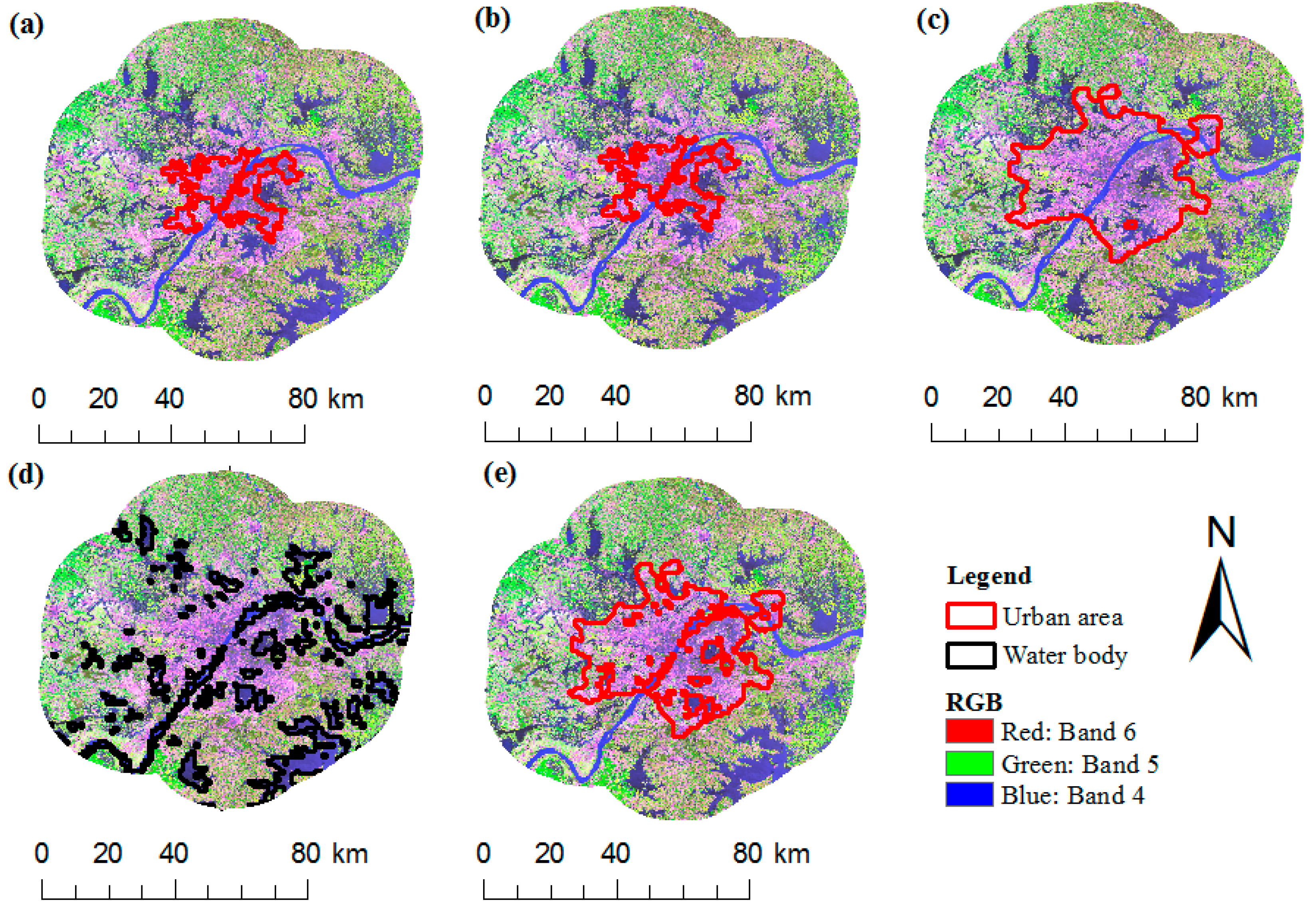
Figure 3.
The comparison of different data and methods of extracting the urban areas or water body in WH: (a) urban areas in WH extracted from MODIS LCD in 2001; (b) urban areas in WH extracted from MODIS LCD in 2013; (c) urban areas in WH extracted from stable nighttime light data in 2013; (d) the union areas of water body in WH extracted from MODIS LCD; (e) SNLD and MODIS LCD were combined to produce the urban areas in WH. The background map was the land surface temperature (LST, °C) in WH in summer, 2013.
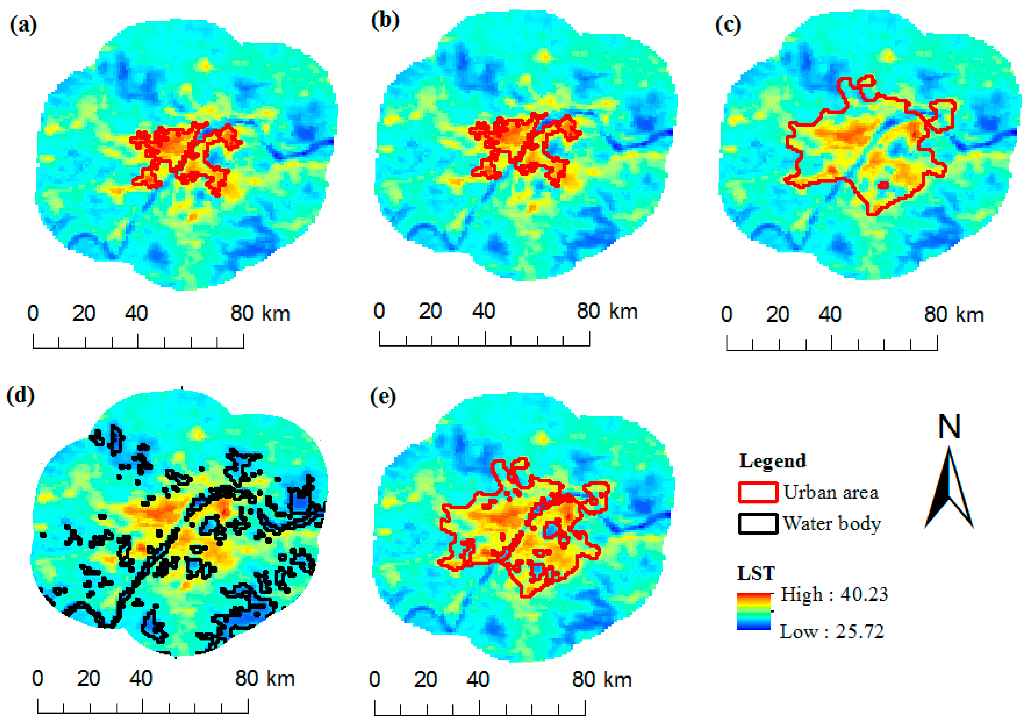
Figure 4.
The temporal trends of ∆EVI averaged for 10 cities during 2001–2016.
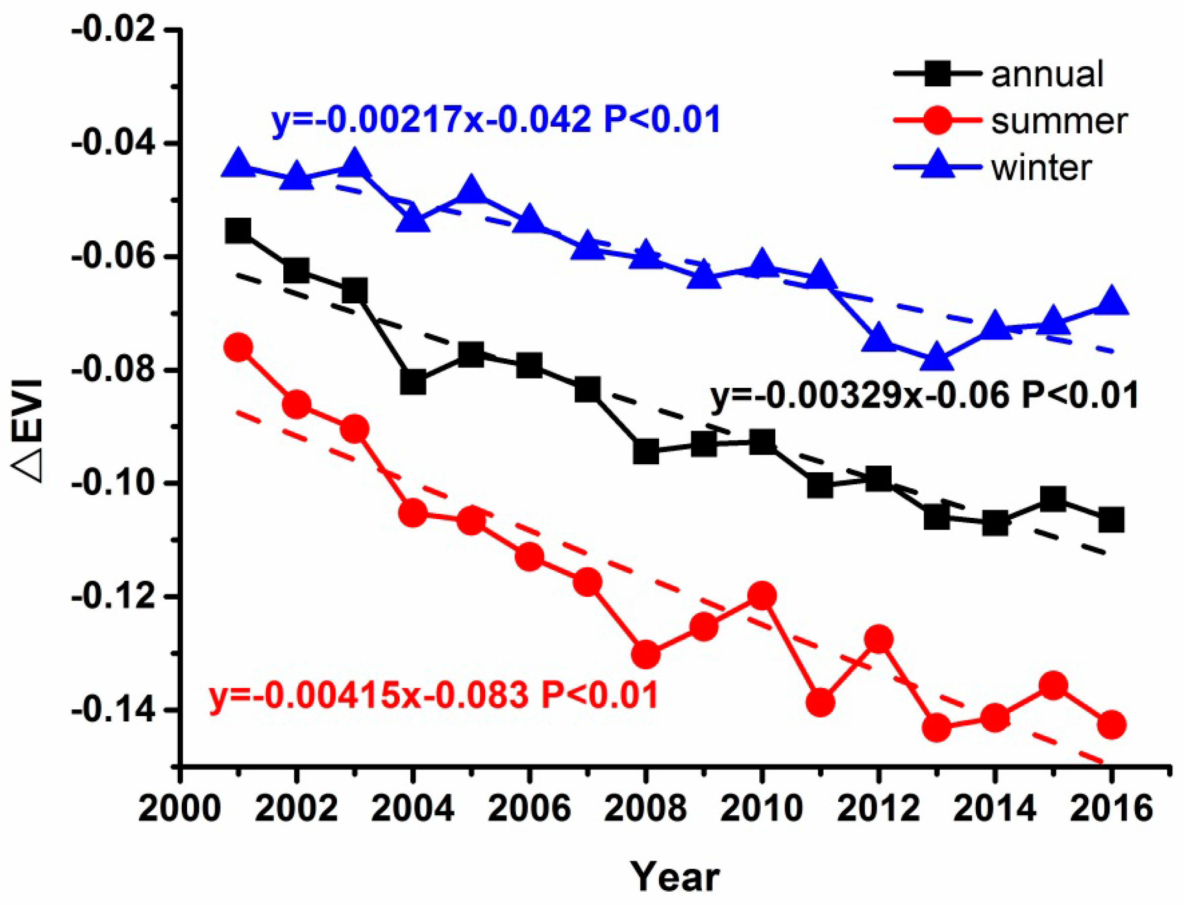
Figure 5.
The temporal trends of daytime SUHII averaged for 10 cities during 2001–2016.

Figure 6.
The temporal trends of nighttime SUHII averaged for 10 cities during 2001–2016.
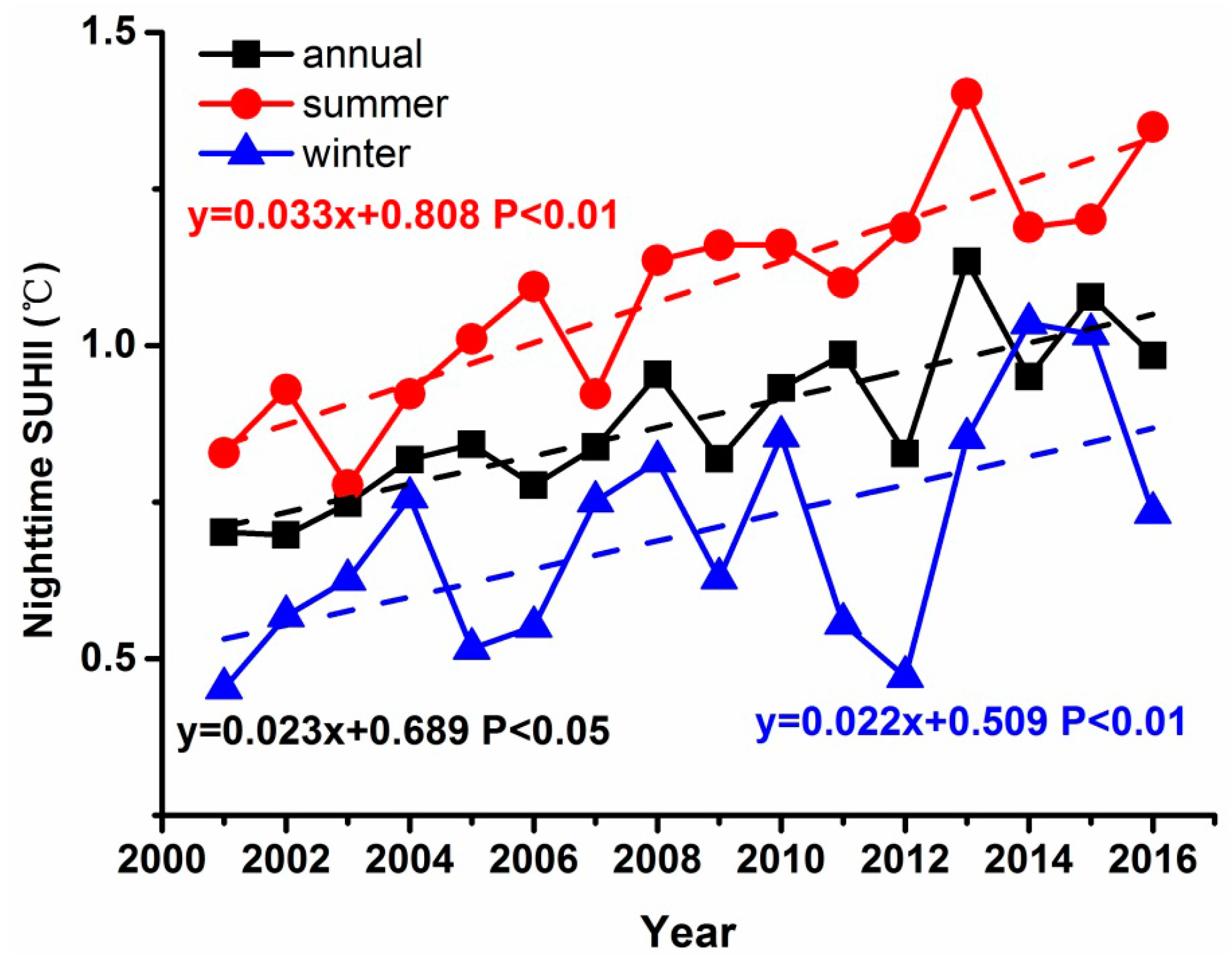
Figure 7.
Correlation analyses between linear slope of SUHII and ∆EVI: (a) annual daytime; (b) annual nighttime; (c) summer daytime; (d) summer nighttime; (e) winter daytime; (f) winter nighttime. Each dot represented a city.
Figure 7.
Correlation analyses between linear slope of SUHII and ∆EVI: (a) annual daytime; (b) annual nighttime; (c) summer daytime; (d) summer nighttime; (e) winter daytime; (f) winter nighttime. Each dot represented a city.


Table 1.
The coefficients of calibration equations for intercalibrating the stable nighttime light (SNLD) data.
Table 1.
The coefficients of calibration equations for intercalibrating the stable nighttime light (SNLD) data.
| Data | C1 | C2 | C3 | R2 |
|---|---|---|---|---|
| F142001 | −0.0176 | 2.0892 | −0.8501 | 0.96 |
| F142002 | −0.0131 | 1.7978 | 0.302 | 0.96 |
| F142003 | −0.0147 | 1.888 | 0.7129 | 0.96 |
| F152001 | −0.0109 | 1.6914 | −1.3106 | 0.94 |
| F152002 | −0.0066 | 1.4128 | −0.5183 | 0.94 |
| F152003 | −0.0182 | 2.1077 | 0.22 | 0.94 |
| F152004 | −0.0178 | 2.0849 | 0.1465 | 0.96 |
| F152005 | −0.0173 | 2.0518 | 0.397 | 0.94 |
| F152006 | −0.0158 | 1.9692 | 0.066 | 0.96 |
| F152007 | −0.0186 | 2.1455 | 0.235 | 0.98 |
| F162004 | −0.0141 | 1.8747 | −0.6434 | 0.94 |
| F162005 | −0.021 | 2.2854 | −0.9842 | 0.95 |
| F162006 | −0.0133 | 1.8456 | −0.8746 | 0.96 |
| F162007 | −0.0098 | 1.6158 | −0.4421 | 0.96 |
| F162008 | −0.0105 | 1.6601 | −0.6306 | 0.96 |
| F162009 | −0.0121 | 1.7534 | 0.4396 | 0.97 |
| F182010 | 0 | 1 | 0 | 1.00 |
| F182011 | −0.0037 | 1.2136 | 0.7621 | 0.97 |
| F182012 | −0.0013 | 1.0635 | 0.5368 | 0.98 |
| F182013 | −0.0006 | 1.0114 | 1.869 | 0.97 |
Table 2.
The amount of urban area in the 10 cities for the year 2001 and 2013. Unit: square kilometer. The numbers in parentheses indicate the area extracted from Landsat data.
Table 2.
The amount of urban area in the 10 cities for the year 2001 and 2013. Unit: square kilometer. The numbers in parentheses indicate the area extracted from Landsat data.
| YRDUA | NJ | HF | WH | CS | NC | CQ | CD | KM | GY | |
|---|---|---|---|---|---|---|---|---|---|---|
| 2001 | 3376 | 489 | 193 | 453 | 191 | 118 | 277 | 387 | 298 | 85 |
| 2002 | 4313 | 646 | 259 | 499 | 216 | 169 | 296 | 423 | 308 | 92 |
| 2003 | 5813 | 842 | 311 | 579 | 312 | 292 | 381 | 598 | 329 | 249 |
| 2004 | 6767 | 948 | 344 | 667 | 390 | 331 | 438 | 677 | 352 | 255 |
| 2005 | 7831 | 1003 | 378 | 748 | 405 | 334 | 489 | 711 | 392 | 259 |
| 2006 | 8389 | 1013 | 413 | 763 | 441 | 341 | 547 | 867 | 423 | 259 |
| 2007 | 8919 | 1077 | 516 | 863 | 521 | 393 | 566 | 909 | 463 | 259 |
| 2008 | 9788 | 1128 | 594 | 893 | 537 | 418 | 568 | 934 | 492 | 259 |
| 2009 | 9840 | 1130 | 602 | 893 | 538 | 418 | 585 | 1100 | 596 | 275 |
| 2010 | 10,847 | 1261 | 690 | 932 | 557 | 429 | 587 | 1248 | 616 | 281 |
| 2011 | 11,873 | 1359 | 763 | 1031 | 568 | 448 | 587 | 1258 | 627 | 299 |
| 2012 | 11,945 | 1360 | 764 | 1031 | 575 | 448 | 614 | 1258 | 680 | 299 |
| 2013 | 13,073 | 1443 (1335) | 844 (584) | 1339 (1088) | 790 (554) | 533 (410) | 808 (716) | 1591 (1317) | 727 (571) | 385 (295) |
Table 3.
16-year averaged urbanization effects (UEs) on vegetation (∆EVI) at 10 cities in Yangtze River Basin (YRB), China. The average data in the table is the mean value of 10 cities.
Table 3.
16-year averaged urbanization effects (UEs) on vegetation (∆EVI) at 10 cities in Yangtze River Basin (YRB), China. The average data in the table is the mean value of 10 cities.
| City | Annual | Summer | Winter |
|---|---|---|---|
| CD | −0.074 | −0.092 | −0.060 |
| CS | −0.106 | −0.153 | −0.072 |
| CQ | −0.101 | −0.157 | −0.069 |
| GY | −0.082 | −0.115 | −0.044 |
| HF | −0.082 | −0.100 | −0.055 |
| KM | −0.115 | −0.126 | −0.105 |
| NC | −0.088 | −0.122 | −0.051 |
| NJ | −0.069 | −0.099 | −0.043 |
| WH | −0.093 | −0.137 | −0.064 |
| YRDUA | −0.071 | −0.087 | −0.042 |
| Average | −0.088 | −0.119 | −0.060 |
Table 4.
16-year averaged surface urban heat island intensity (SUHII) at 10 cities in YRB, China.
| City | Annual Day (°C) | Annual Night (°C) | Summer Day (°C) | Summer Night (°C) | Winter Day (°C) | Winter Night (°C) |
|---|---|---|---|---|---|---|
| CD | 2.26 | 0.71 | 3.00 | 1.28 | 1.13 | 0.80 |
| CS | 1.47 | 0.56 | 3.29 | 1.12 | −0.16 | 0.08 |
| CQ | 1.70 | 0.81 | 3.02 | 1.51 | 0.46 | 0.27 |
| GY | 1.96 | 1.26 | 2.79 | 1.57 | 1.04 | 0.60 |
| HF | 1.43 | 0.29 | 2.79 | 0.45 | 0.08 | −0.07 |
| KM | 2.69 | 1.83 | 4.49 | 2.36 | 1.38 | 1.25 |
| NC | 1.18 | 0.72 | 3.37 | 0.82 | −0.33 | 0.88 |
| NJ | 1.15 | 0.76 | 2.77 | 0.30 | 0.06 | 0.95 |
| WH | 0.71 | 0.84 | 2.43 | 0.76 | −0.46 | 0.84 |
| YRDUA | 1.75 | 1.02 | 2.74 | 0.70 | 0.87 | 1.39 |
| Average | 1.63 | 0.88 | 3.07 | 1.09 | 0.41 | 0.70 |
Table 5.
Temporal trends of ∆EVI at 10 cities in YRB, China.
| City | Annual (/Year) | Summer (/Year) | Winter (/Year) |
|---|---|---|---|
| CD | −0.00538 ** | −0.00563 ** | −0.00607 ** |
| CS | −0.00460 ** | −0.00630 ** | −0.00310 ** |
| CQ | −0.00529 ** | −0.00614 ** | −0.00390 ** |
| GY | −0.00336 ** | −0.00508 ** | −0.00171 ** |
| HF | −0.00392 ** | −0.00572 ** | −0.00220 |
| KM | −0.00308 ** | −0.00247 | −0.00257 ** |
| NC | −0.00216 | −0.00487 ** | −0.00083 |
| NJ | −0.00110 ** | −0.00044 | 0.00009 |
| WH | −0.00189 ** | −0.00376 ** | −0.00084 |
| YRD | −0.00211 ** | −0.00113 | −0.00051 |
| Average | −0.00329 ** | −0.00415 ** | −0.00217 ** |
Significance levels: ** p < 0.01.
Table 6.
Temporal trends of ∆EVI and SUHII in old urban areas (OUAs) in the YRB, China.
| City | Annual Daytime SUHII (°C/Year) | Annual Nighttime SUHII (°C/Year) | Annual ∆EVI (/Year) |
|---|---|---|---|
| CD | 0.020 | 0.020 | −0.00285 ** |
| CS | 0.045 ** | 0.052 ** | −0.00303 ** |
| CQ | 0.082 ** | 0.053 ** | −0.00388 ** |
| GY | 0.027 | 0.006 | −0.00229 ** |
| HF | 0.014 | 0.065 ** | −0.00276 ** |
| KM | 0.029 | 0.024 ** | −0.00148* |
| NC | 0.029 * | −0.003 | −0.00154 ** |
| NJ | 0.031 * | 0.025 | −0.00017 |
| WH | 0.033 | 0.012 | −0.00126 * |
| YRD | 0.033 | 0.014 | −0.00160 * |
| Average | 0.034 ** | 0.027 ** | −0.00209 ** |
Significance levels: * p < 0.05, ** p < 0.01.
Table 7.
Temporal trends of SUHII at 10 cities in YRB, China.
| City | Annual Day (°C/Year) | Annual Night (°C/Year) | Summer Day (°C/Year) | Summer Night (°C/Year) | Winter Day (°C/Year) | Winter Night (°C/Year) |
|---|---|---|---|---|---|---|
| CD | 0.107 ** | 0.014 | 0.233 ** | 0.003 | 0.015 | 0.005 |
| CS | 0.099 ** | 0.040 ** | 0.162 ** | 0.057 ** | 0.074 * | 0.038 |
| CQ | 0.117 ** | 0.041 ** | 0.140 ** | 0.086 ** | 0.134 ** | 0.047 ** |
| GY | 0.040 * | 0.018 | 0.094 ** | 0.014 | 0.002 | 0.003 |
| HF | 0.100 ** | 0.036 ** | 0.231 ** | 0.016 | 0.006 | 0.019 |
| KM | 0.034 * | 0.036 ** | 0.037 | 0.053 ** | 0.002 | 0.034 ** |
| NC | 0.075 ** | 0.004 | 0.196 ** | 0.037 * | 0.013 | 0.039 |
| NJ | 0.062 ** | 0.018 | 0.107 ** | 0.015 | 0.005 | 0.037 * |
| WH | 0.068 ** | 0.001 | 0.122 ** | 0.038 * | 0.038 ** | 0.008 |
| YRDUA | 0.072 ** | 0.007 | 0.122 * | 0.018 | 0.002 | 0.013 |
| Average | 0.077 ** | 0.033 ** | 0.144 ** | 0.023 ** | 0.029 ** | 0.022 * |
Significance levels: * p < 0.05, ** p < 0.01.
Table 8.
Correlation analyses between SUHII and ∆EVI at 10 cities in YRB, China.
| City | Annual Day | Annual Night | Summer Day | Summer Night | Winter Day | Winter Night |
|---|---|---|---|---|---|---|
| CD | −0.882 ** | −0.236 | −0.953 ** | −0.203 | 0.006 | 0.106 |
| CS | −0.887 ** | −0.702 ** | −0.873 ** | −0.710 ** | −0.438 | −0.715 ** |
| CQ | −0.895 ** | −0.709 ** | −0.912 ** | −0.828 ** | 0.388 | −0.621 * |
| GY | −0.474 | −0.301 | −0.315 | −0.181 | −0.266 | −0.149 |
| HF | −0.869 ** | −0.682 ** | −0.896 ** | −0.155 | 0.056 | 0.099 |
| KM | −0.598 * | −0.886 ** | −0.364 | −0.372 | −0.144 | −0.749 ** |
| NC | −0.442 | −0.368 | −0.810 ** | −0.529 * | 0.450 | −0.612 * |
| NJ | −0.560 * | −0.512 * | −0.348 | 0.207 | 0.005 | −0.238 |
| WH | −0.618 * | −0.237 | −0.637 ** | −0.693 ** | −0.287 | −0.490 |
| YRD | −0.672 ** | −0.360 | −0.406 | −0.544 * | 0.103 | −0.076 |
| Average | −0.932 ** | −0.859 ** | −0.919 ** | −0.877 ** | −0.696 ** | −0.547 * |
Significance levels: * p < 0.05, ** p < 0.01.
© 2017 by the authors. Licensee MDPI, Basel, Switzerland. This article is an open access article distributed under the terms and conditions of the Creative Commons Attribution (CC BY) license (http://creativecommons.org/licenses/by/4.0/).
Share and Cite
MDPI and ACS Style
Yao, R.; Wang, L.; Gui, X.; Zheng, Y.; Zhang, H.; Huang, X. Urbanization Effects on Vegetation and Surface Urban Heat Islands in China’s Yangtze River Basin. Remote Sens. 2017, 9, 540. https://doi.org/10.3390/rs9060540
AMA Style
Yao R, Wang L, Gui X, Zheng Y, Zhang H, Huang X. Urbanization Effects on Vegetation and Surface Urban Heat Islands in China’s Yangtze River Basin. Remote Sensing. 2017; 9(6):540. https://doi.org/10.3390/rs9060540
Chicago/Turabian StyleYao, Rui, Lunche Wang, Xuan Gui, Yukun Zheng, Haoming Zhang, and Xin Huang. 2017. "Urbanization Effects on Vegetation and Surface Urban Heat Islands in China’s Yangtze River Basin" Remote Sensing 9, no. 6: 540. https://doi.org/10.3390/rs9060540
Note that from the first issue of 2016, this journal uses article numbers instead of page numbers. See further details here.