Optimizing Semi-Analytical Algorithms for Estimating Chlorophyll-a and Phycocyanin Concentrations in Inland Waters in Korea

Abstract

Several semi-analytical algorithms have been developed to estimate the chlorophyll-a (Chl-a) and phycocyanin (PC) concentrations in inland waters. This study aimed at identifying the influence of algorithm parameters on the output variables and searching optimal parameter values. The optimal parameters of seven semi-analytical algorithms were applied to estimate the Chl-a and PC concentrations. The absorption coefficient measurements were coupled with pigment measurements to calibrate the algorithm parameters. For sensitivity analysis, the elementary effect test was conducted to analyze the influence of the algorithm parameters. The sensitivity analysis results showed that the parameters in the Y function and specific absorption coefficient were the most sensitive parameters. Then, the parameters were optimized via a single-objective optimization that involved one objective function being minimized and a multi-objective optimization that contained more than one objective function. The single-objective optimization led to substantial errors in absorption coefficients. In contrast, the multi-objective optimization improved the algorithm performance with respect to both the absorption coefficient estimates and pigment concentration estimates. The optimized parameters of the absorption coefficient reflected the high-particulate content in waters of the Baekje reservoir using an infrared backscattering wavelength and relatively high value of Y. Moreover, the results indicate the value of measuring the site-specific absorption if site-specific optimization of semi-analyical algorithm parameters was envisioned.

1. Introduction

Harmful algal blooms (HABs) create formidable problems for freshwater aquatic ecosystems and human health. HABs cause the depletion of dissolved oxygen, resulting in the death of aquatic animals and toxin production [1]. To address these problems, it is essential to understand the spatial and temporal distributions of HABs and the effects of the blooms on aquatic ecosystems. Essentially, the implementation of effective monitoring strategies is required to identify HABs.

Remote sensing techniques are utilized to detect HABs and quantify an algal biomass using the chlorophyll-a (Chl-a) concentration, which is an indicator of a phytoplankton biomass [2,3], and the phycocyanin (PC) concentration, which is an accessory pigment of cyanobacteria [4]. In inland waters, several algorithms are applied to estimate the Chl-a concentration [5,6,7,8,9,10,11,12,13] and PC concentration [13,14,15]. However, these algorithms have limitations due to the variation of optical properties among water systems [16]. To account for this variation, the absorption coefficient as an inherent optical property (IOP) is included in equations to estimate the concentrations of Chl-a and PC. The absorption coefficient effectively accounts for the properties of the particulate and dissolved organic matter in the water.

Semi-analytical bio-optical algorithms have been developed for estimating Chl-a and PC concentrations in inland waters. These algorithms were modified for different inland waters because of the differences in their optical properties. In general, inland waters appeared to be optically complex due to a wide variability in the concentrations of pigments, suspended sediments, and colored dissolved organic matter [17]. The variation in the absorption coefficient was recognized as a consequence of such complexity. To account for this optical complexity, the absorption coefficient was included in the semi-analytical algorithms.

The measured absorption coefficient was used to improve the performance of the algorithms [9]. Given the absorption coefficients, the algorithm’s performance could be evaluated by its ability to estimate both biomass concentrations and absorption coefficients. However, sensitivity analysis of the semi-analytical algorithm parameters has rarely been implemented [9]. It is very important to understand how the uncertainty in estimation of both biomass concentrations and absorption coefficients can be attributed to different sources of uncertainty in its parameters.

The optimization of the semi-analytical algorithm’s parameters was required because of the site-specific properties of waters. However, parameter optimization in the semi-analytical algorithms in inland waters relied on the algorithms performance to estimate the Chl-a and PC concentrations [5,6,13,14]. The absorption coefficient has been previously estimated [9,14] and used to compute pigment concentration without site-specific changes in the semi-analytical algorithms.

Therefore, the objectives of this study were to (1) identify the influences of semi-analytical algorithm parameters on the estimation of both absorption coefficient and pigment concentration; (2) calibrate the algorithm’s parameters using single- and multi-objective optimization methods; and (3) assess the effect of measured absorption coefficients in multi-objective parameter optimization for semi-analytical algorithms on the accuracy of those algorithms.

2. Materials and Methods

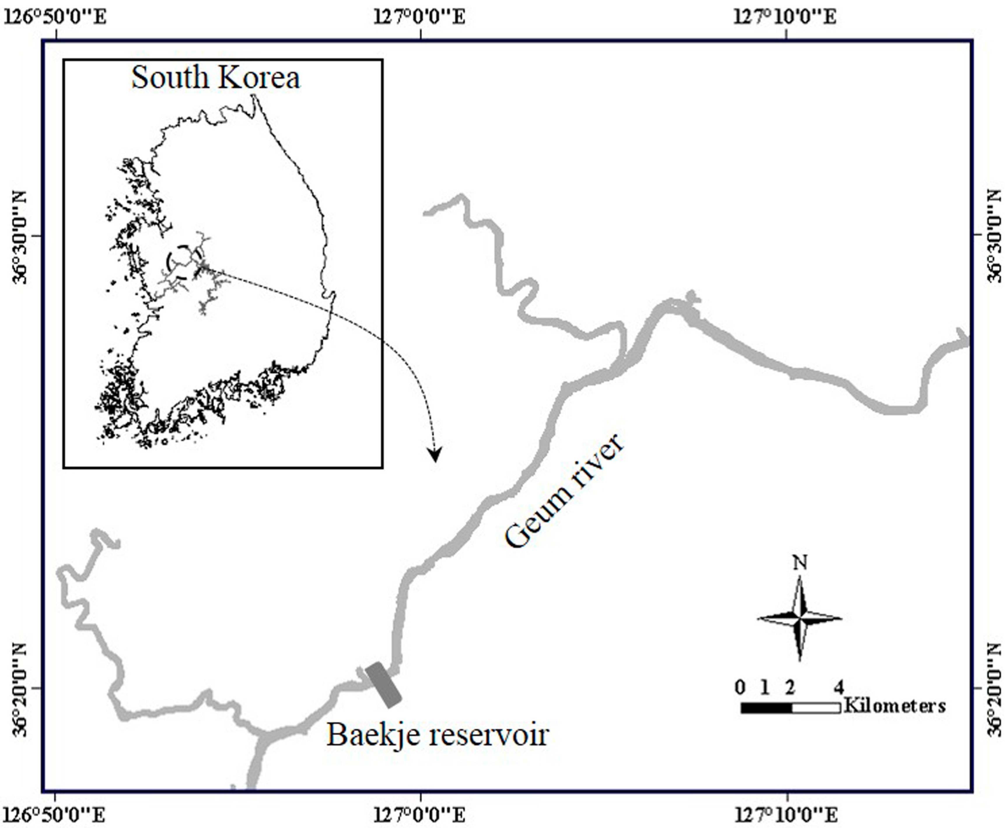
2.1. Study Site

The Baekje reservoir (36°32′N 126°94′E) is located in the main stream of the Geum River (Figure 1). The Geum River is one of the largest rivers in Korea and contains the Sejong, Gongju, and Baekje reservoirs. The average depth of the Baekje reservoir is 4 m. The length of the reservoir is 23 km. Drinking water, agriculture water, and electricity have been supplied from the Baekje reservoir [18].

Algal blooms frequently occurred in the Baekje reservoir due to an increase in the water retention time, nutrient loads from the tributary in urban areas, and climate change [18]. In addition, the algal blooms in the Baekje reservoir were the cyanobacteria-dominant blooms that were harmful to human health and aquatic life due to the production of cyanotoxins [19]. Thus, this type of algal bloom posed significant challenges in terms of water supply and aquatic ecosystem [5].

2.2. Field Monitoring and Experiment

In this study, eight field-sampling events were conducted from June to October in 2016. The monitoring distance was approximately 10–15 km, which started from the dam of the Baekje reservoir. Nearly 20 sampling points were collected in each monitoring event. In each sampling point, the water samples were collected and the remote sensing reflectance was measured. For analyzing cyanobacteria, netting was used to concentrate the water samples.

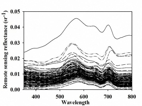
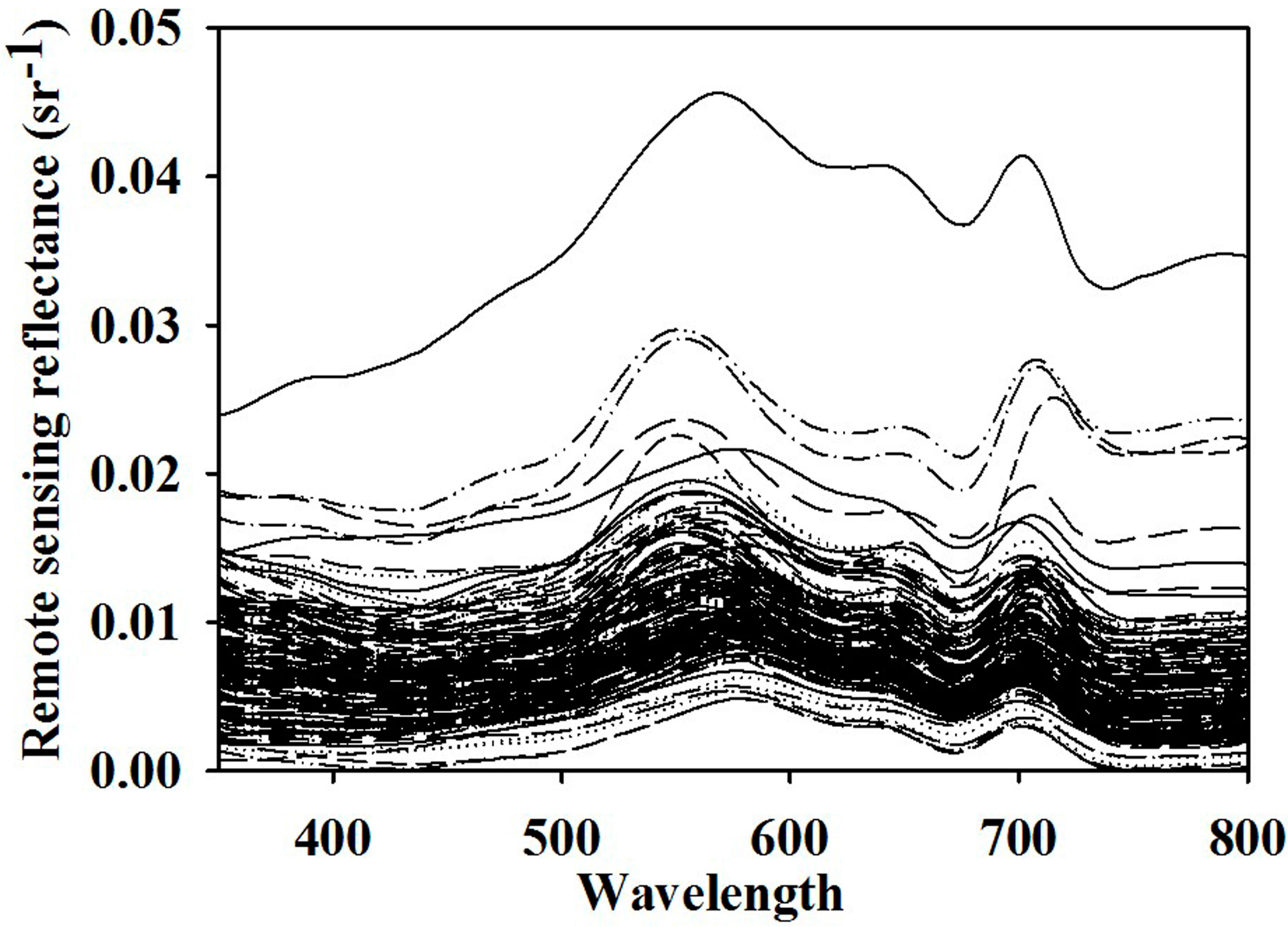
2.2.1. Remote Sensing Reflectance Retrieval

The remote sensing reflectance $R_{rs}$ was measured on the water surface by using a FieldSpec HandHeld 2 spectroradiometer (ASD Inc., Boulder, CO, USA) having a wavelength range of 325–1075 nm in Figure 2. The measuring position had an azimuth angle of 130–135° and a zenith angle of 35–40°, which was used to decrease sun glint and shading interference [9,13]. The irradiance and radiance $L_W$ on the water surface were collected to evaluate $R_{rs}$ and had the following ratio:

$$R_{rs}\left(\lambda \right)=\frac{L_w\left(\lambda \right)}{L_E\left(\lambda \right)}.$$

(1)

The radiance of water $L_W$ was defined to minimize the sky effect [13]:

$$L_w\left(\lambda \right)=L_{w.r}\left(\lambda \right)-q{L}_{sky}\left(\lambda \right),$$

(2)

where $L_{w.r}\left(\lambda \right)$ is the radiance from water with the sky effect, and $L_{sky}\left(\lambda \right)$ is the radiance from the sky, and q was the skylight interference between water and air, which is defined as 0.025.

2.2.2. Extraction of Chl-a and PC

The standard method was referenced to analyze the Chl-a concentration in the water samples [20]. The extraction processes of Chl-a were the following: the water samples were filtered with a glass microfiber filter (Whatman) that had a 0.7-μm pore size. The filtered samples were ground and stayed in an acetone and water (9:1) solution for 24 h. Then, the optical densities of the sample supernatants were measured using the Cary-5000 UV-Vis-NIR spectrophotometer (Agilent Inc., Santa Clara, CA, USA) that provided a wavelength range from 200 to 3300 nm. From the optical densities data, the estimation of Chl-a concentration was followed by [21].

PC extraction was based on the findings of [22,23]. The water samples netted approximately 10⁶ cyanobacteria cells per milliliter and were homogenized with an Ultra-Sonicator (Sonictopia Inc., Cheongju, Korea). The homogenized samples of 30 mL were centrifuged at 4000 rpm and 5 °C for 15 min. The pellets of the centrifuged samples remained without the supernatants. A 5-mL phosphate buffer solution was added to the samples. The samples were frozen at −20 °C for 24 h and then thawed at room temperature to break the PC pigment cells. A shaking incubator (N-BIOTEK Inc., Bucheon, Korea) was used to release the PC pigment from the cells at 150 rpm for 15 min. The centrifuging process was repeated under the same condition with the prior step to analyze the supernatants. A Cary-5000 UV-Vis-NIR spectrophotometer was used to measure the optical densities of the supernatant samples. Then, the PC concentration was estimated using the following equation:

$$PC\left(mg·m^{-3}\right)=\frac{O{D}_{620}-\left(0.474\times O{D}_{652}\right)}{5.34},$$

(3)

where $O{D}_{620}$ and $O{D}_{652}$ were the optical density at wavelengths 620 nm and 652 nm, respectively.

2.2.3. Absorption Coefficient Analysis of Phytoplankton

The phytoplankton pigment on the GF/F filter was directly measured using the Cary-5000 UV-Vis-NIR spectrophotometer equipped with an integrating sphere accessory. This method was referred to as the light transmission measurement, and allowed the retrieval of absorption coefficients of in vivo phytoplankton pigments without non-algal particle pigments [24]. The integrating sphere was attached inside the spectrophotometer and had a 25-mm diameter in a dual-beam port. When the filtered sample was placed into the reflectance and transmittance ports, the reflectance and transmittance of the sample filters were measured, respectively. The wavelength range for the reflectance and transmittance data was set from 350 to 800 nm with a 1-nm interval. To obtain the pigment information of a non-algal particle, a 5% NaClO solution bleached the phytoplankton pigment on the sample filters. The transmittance and reflectance of the bleached samples were measured. The transmittance and reflectance measurements were repeated with hydrated reference filters. The transmittance and reflectance data were converted into optical densities for both cases before and after bleaching. In this study, specific equations of absorption coefficient conversion reported previously was followed [24]. An evaluation of the absorption coefficient of the filter sample was previously introduced [25]:

$$a_f\left(\lambda \right)=\frac{2.303A}{\epsilon V}\left(O{D}_f\left(\lambda \right)-O{D}_r\left(\lambda \right)-O{D}_n\right),$$

(4)

where $a_f\left(\lambda \right)$ is absorption coefficient of the filter sample, A is the filtered surface area, V is filtered water volume, ε is a scaling factor, $O{D}_f\left(\lambda \right)$ is the optical density of the filter sample, $O{D}_r\left(\lambda \right)$ is the optical density of the reference filter, and $O{D}_n$ is the optical density when the absorption coefficient was minimum.

The absorption coefficient of the in vivo phytoplankton was estimated by subtracting it from that of the non-algal particle.

2.3. Semi-Analytical Algorithms for Inland Water

The IOPs such as absorption and backscattering were utilized to construct semi-analytical algorithms that estimate the Chl-a and PC concentrations. In this study, two types of semi-analytical algorithms were estimated using a wavelength-dependent backscattering coefficient and a wavelength-independent backscattering coefficient. The algorithms below were referenced by the name of the first author of the publication wherein the algorithm appeared.

This study followed the IOP Inversion Model of Inland Waters (IIMIW) developed by [9]. The IIMIW assumed that the backscattering coefficient was dependent on the wavelength and was divided into backscattering of water and particles:

$$b_b\left(\lambda \right)=b_p\left(560\right){\left(\frac{560}{\lambda }\right)}^Y+b_w\left(\lambda \right),$$

(5)

where $b_b\left(\lambda \right)$ is the backscattering coefficient, $b_p\left(\lambda \right)$ is the backscattering coefficient of the particles, $b_w\left(\lambda \right)$ is the backscattering coefficient of water, and ^Y is an empirical constant.

$b_p\left(560\right)$ was calculated by

$$b_p\left(560\right)=\frac{b_{bp}\left(778\right)-b_w\left(778\right)}{{\left(\frac{560}{778}\right)}^Y},$$

(6)

$$b_{bp}\left(778\right)=\frac{r_{rs}\left(778\right)a_w\left(778\right)}{0.082-r_{rs}\left(778\right)},$$

(7)

$$Y=2.0\left(1-1.2exp\left(-xp·\frac{r_{rs}\left(443\right)}{r_{rs}\left(560\right)}\right)\right),$$

(8)

where $r_{rs}\left(\lambda \right)$ is the remote sensing reflectance underneath the water surface and is set to 1.85$R_{rs}\left(\lambda \right)$, $b_{bp}\left(778\right)$ is the particle backscattering coefficient at a wavelength of 778 nm, and $a_w\left(\lambda \right)$ is the absorption coefficient of water.

The reflectance ratio was utilized previously [9] to estimate the absorption coefficient and this could be expressed as follows:

$$a_g\left({\lambda }_1\right)=[\frac{R\left({\lambda }_2\right)b_b\left({\lambda }_1\right)}{R\left({\lambda }_1\right)b_b\left({\lambda }_2\right)}\left({\mathrm{a}}_{\mathrm{w}}\left({\lambda }_2\right)+b_b\left({\lambda }_2\right)\right]-b_b\left({\lambda }_1\right)-a_w\left({\lambda }_1\right),$$

(9)

where $a_g\left({\lambda }_1\right)$ is the absorption coefficient without the water effect, ${\lambda }_2$ is set to 709 nm [5,9,13,14,26], and $a_w\left(\lambda \right)$ and $b_w\left(\lambda \right)$ are constants whose values were set as per those used by [27].

The absorption coefficient of PC was obtained [14] by partitioning $a_g\left(\lambda \right)$ to the absorption coefficient of colored dissolved organic matter (CDOM), PC, and phytoplankton with PC influence. The phytoplankton absorption coefficient can be expressed as follows:

$$a_{phy}\left(\lambda \right)=a_g\left(\lambda \right)-a_{cdom}\left(\lambda \right).$$

(10)

The absorption coefficient of CDOM can be expressed as follows:

$$a_{cdom}\left(412\right)=a_g\left(412\right)-a_{phy-pc}\left(412\right),$$

(11)

$$a_{cdom}\left(510\right)=a_g\left(510\right)-a_{phy-pc}\left(510\right),$$

(12)

$$S_{cdom}=\frac{1}{98}\ln \left(\frac{a_{cdom}\left(412\right)}{a_{cdom}\left(510\right)}\right),$$

(13)

$$a_{cdom}\left(\lambda \right)=a_{cdom}\left(412\right)\exp \left(-S_{cdom}\left(\lambda -412\right)\right),$$

(14)

where $a_{cdom}\left(412\right)$ and $a_{cdom}\left(510\right)$ are the absorption coefficients at 412 and 510 nm, respectively. $a_{phy - pc}\left(\lambda \right)$ is the absorption coefficient of phytoplankton without the PC effect, $S_{cdom}$ is the CDOM spectral slope, and $a_{cdom}\left(\lambda \right)$ is the absorption coefficient of CDOM along the wavelength.

Here, the absorption coefficient of phytoplankton without the PC effect was calculated using the following equation:

$$a_{phy - pc}\left(\lambda \right)=C_1\left(\lambda \right)a_g\left(675\right)+C_2\left(\lambda \right),$$

(15)

where $C_1\left(\lambda \right)$ and $C_2\left(\lambda \right)$ are the regression coefficients between the observed absorption coefficients and the absorption coefficient at 675 nm.

Finally, the absorption coefficient of PC could be evaluated as follows:

$$a_{pc}\left(\lambda \right)={\mathrm{a}}_{\mathrm{phy}}\left(\lambda \right)-a_{phy - pc}\left(\lambda \right),$$

(16)

where $a_{pc}\left(\lambda \right)$ is the absorption coefficient of PC and the wavelength $\lambda$ is set to 620 nm for PC [12,14,28].

Another method for IOP estimation was based on the assumption that backscattering was independent of the wavelength and was developed by [29]. The backscattering coefficient can be expressed as follows:

$$b_b\left(778\right)=\frac{1.61R_{rs}\left(778\right)}{0.082-0.6R_{rs}\left(778\right)}.$$

(17)

The absorption coefficient is defined as follows:

$$a_g\left({\lambda }_1\right)=\frac{R_{rs}\left({\lambda }_2\right)}{R_{rs}\left({\lambda }_1\right)}\left(a\left({\lambda }_2\right)+b_b\right)-b_b-a_w\left({\lambda }_1\right),$$

(18)

where ${\lambda }_1$ is 665 nm for Chl-a-sensitive wavelength and ${\lambda }_2$ is 709 nm. They were the same for the IIMIW algorithm.

Based on the IIMIW, Gons, Gilerson, and Ritchie algorithms were used to estimate the Chl-a concentration.

The Gons algorithm is expressed as follows:

$$Chl-a\left(mg m^{-3}\right)=\frac{a_g\left({\lambda }_{chla}\right)}{a_g^{*}\left({\lambda }_{chla}\right)},$$

(19)

where ${\lambda }_{chla}$ is 665 nm for the Chl-a-sensitive wavelength and $a_g^{*}\left({\lambda }_{chla}\right)$ is the specific absorption coefficient (m² mg⁻¹) that has a reference value of 0.0161 m² mg⁻¹.

The Gilerson algorithm is expressed as follows:

$$Chl-a\left(mg m^{-3}\right)={\left(\frac{a_g\left({\lambda }_{chla}\right)}{a_g^{*}\left({\lambda }_{chla}\right)}\right)}^{1.124},$$

(20)

where the specific absorption coefficient is set to 0.022 m² mg⁻¹.

The Ritchie algorithm can be expressed as follows:

$$Chl-a\left(mg m^{-3}\right)=4.34(-0.3319a_{gh}\left(630\right)-1.7485a_{gh}\left(647\right)+11.9442a_{gh}\left({\lambda }_1\right)-0.3319a_{gh}\left(630\right)),$$

(21)

where ${\mathit{a}}_{\mathit{g}}\left(\mathit{\lambda }\right)$ is set to 1.47${\mathit{a}}_{\mathit{g}}\left(\mathit{\lambda }\right)$ to amplify the signal of the absorption coefficient, as suggested by [13].

Additionally, Ref. [9] utilized the reflectance ratio to estimate the absorption coefficient and it can be expressed as follows:

$$PC \left(mg m^{-3}\right)=\frac{a_{pc}\left({\lambda }_{pc}\right)}{a_{pc}^{*}\left({\lambda }_{pc}\right)},$$

(22)

where ${\lambda }_{pc}$ is 620 nm for the PC-sensitive wavelength and $a_{pc}^{*}\left({\lambda }_{pc}\right)$ has a constant value of 0.007 m² mg⁻¹.

The Duan and Simis algorithms were introduced by the backscattering-independent model with respect to the wavelengths. These algorithms were used to estimate the Chl-a concentration.

The Duan algorithm can be expressed as follows:

$$a_g\left({\lambda }_{chla}\right)=\frac{R_{rs}\left(709\right)}{R_{rs}\left({\lambda }_{chla}\right)}\left(a_w\left(709\right)+b_b\right)-{\mathrm{b}}_{\mathrm{b}}^{1.062}-a_w\left({\lambda }_{chla}\right),$$

(23)

$$Chl-a\left(mg m^{-3}\right)=\frac{a_g\left({\lambda }_{chla}\right)}{a_g^{*}\left({\lambda }_{chla}\right)},$$

(24)

where $a_g^{*}\left({\lambda }_{chla}\right)$ is 0.161 m² mg⁻¹.

The Simis algorithm can be expressed as follows:

$$a_g\left({\lambda }_{chla}\right)=\frac{1}{0.68}\left(\frac{R_{rs}\left(709\right)}{R_{rs}\left({\lambda }_{chla}\right)}\left(a_w\left(709\right)-b_b\right)-b_b-a_w\left({\lambda }_{chla}\right)\right),$$

(25)

$$Chl-a\left(mg m^{-3}\right)=\frac{a_g\left({\lambda }_{chla}\right)}{a_g^{*}\left({\lambda }_{chla}\right)},$$

(26)

where $a_g^{*}\left({\lambda }_{chla}\right)$ is 0.0343 m² mg⁻¹.

All processes were summarized in Tables S1 and S2 for Chl-a and PC, respectively.

2.4. Global Sensitivity Analysis

The sensitivity analysis was implemented to identify uncertainty and the parameter relations in the semi-analytical algorithms. The elementary effect test (EFT) was employed to accomplish the sensitivity analysis for the parameters inside the algorithms. The parameters included the empirical constant as well as the wavelengths. The EFT was also referred to as the Morris screening method [30]. He introduced the “one-factor-at-a-time” design wherein an input was randomly sampled. The Latin hypercube design was also used for the input screening process. The EFT can be expressed as follows:

$$e_i\left(x\right)=\frac{y^{*}\left(x_1,x_2,\dots x_i+\mathrm{\Delta },\dots x_k\right)-y\left(x\right)}{\mathrm{\Delta }},$$

(27)

where y* is the new outcome, y is the original outcome, and ∆ is the increment dependent on the range of $x_i$ values and the number of discretization increments across the range of $x_i$. We used the MATLAB software to provide the global sensitivity analysis [31]. Elementary effects were computed for all parameters in each Latin hypercube sampling point. The mean and standard deviation of the distribution of the elementary effect were used as metrics to determine the significance of the input parameters. The mean of the elementary effect values indicated the influence of a parameter on the Chl-a and PC concentrations. The standard deviation represented the interaction of a parameter with other parameters [32,33]. The ranking of the means of the elementary effect values provided the sensitivity ranks for parameters.

2.5. Parameter Optimization

This study implemented the optimization of parameters of the semi-analytical algorithms with the single- and multi-objective optimization methods. The pattern search algorithm was employed for performing single-objective optimization using patternsearch.m in MATLAB. The root-mean-square error (RMSE) for the concentrations of the Chl-a and PC algorithms was minimized. The multi-objective optimization method provided a group of optimal points called the Pareto-front optimal set. We used two objective functions: one for the absorption coefficient and the other for the Chl-a and PC concentrations. Both objective functions of the multi-objective algorithm were RMSEs. The multi-objective optimization was performed using gamultiobj.m in MATLAB. Both the pattern search and multi-objective optimizations were applied for each algorithm (i.e., Gons, Gilerson, Ritchie, Duna, Simis, Li, and Simis (PC) algorithms). The parameter ranges were consistent with those of the sensitivity analysis.

A statistical comparison of slopes of “measured vs. estimated” regression lines with unity was performed to evaluate the probability that the estimated results were on the 1:1 line. The t-statistic was used to determine the significance of the regression coefficients, as suggested by [34]. The probability value was calculated using the TTEST function in Excel.

3. Results

3.1. Temporal Variability of Chl-a and PC

The experimental results for the Chl-a and PC concentrations showed a temporal variation from June to October (Figure S1). The intense bloom occurred in the middle of August when both Chl-a and PC had maximum concentrations. In this period, the concentration level of PC significantly increased, indicating that the water body had the cyanobacteria-dominant bloom (

Table 1. Measurements of the pigment concentrations in the Baekje reservoir.

	Mean	Max. †	Min. †	Mean	Max	Min
		Chl-a (mg m−3)			PC (mg m−3)
06.10.2016	39.27 ± 7.48 ‡	52.86	24.89	0.18 ± 0.11	0.45	0
08.05.2016	36.49 ± 15.80	66.18	14.19	29.64 ± 24.16	104.28	6.25
08.12.2016	92.34 ± 51.91	243.14	33.94	169.72 ± 235.61	1014.35	32.63
08.19.2016	37.24 ± 8.02	61.44	25.95	38.07 ± 23.58	100.00	12.25
08.24.2016	32.06 ± 11.27	50.01	14.75	17.16 ± 24.84	95.28	1.96
09.06.2016	25.51 ± 11.32	60.88	11.85	1.23 ± 0.27	1.64	0.83
09.26.2016	29.12 ± 11.35	58.26	19.58	0.89 ± 0.62	3.35	0.52
10.14.2016	27.80 ± 9.33	46.17	13.74	0.36 ± 0.21	0.90	0.19
Total	38.93 ± 27.10	243.14	11.85	29.15 ± 91.50	1014.35	0

^† Max. and Min. indicate maximum and minimum, respectively. ^‡ The “±” sign separates the estimates of averages and standard deviations.

). After August, the PC concentration nearly disappeared. In contrast, the Chl-a concentration maintained a similar level throughout the sampling period.

3.2. Sensitivity of Parameters in Semi-Analytical Algorithms

Steps of the algorithms listed in Equations (1)–(26) (summarized in Tables S1 and S2 in Supplementary Materials) were renamed to have a uniform notation from P1 to P31. The semi-analytical algorithm relations with the renamed parameters are shown in Supplementary A1.

Parameters P1–P13 were related to the estimated IOPs. The other parameters were related to the estimated Chl-a and PC concentrations. The Gons, Gilerson, Ritchie, and Li algorithms had common parameters from P1 to P6 in the semi-analytical algorithm. Ranges of parameter values applied to the EFT were set as summarized in

Table 2. Ranges of the selected parameters for the sensitive analysis and the optimization.

	Parameter	Range	Earlier Published	Unit	Reference
Semi-analytical algorithm for Chl-a	$P_1$	560–720	560	nm	[37]
	$P_2$	0.1–6.0	2.0	-	[38]
	$P_3$	0.1–4.0	1.0	-
	$P_4$	−3.0–−0.1	−1.2	-
	$P_5$	−1.0–−0.1	−0.9	-
	$P_6$	400–500	443	nm
Semi-analytical algorithm for PC	$P_7$	400–500	412	nm	[14]
	$P_8$	501–600	510	nm
	$P_9$	1–100	98	-
	$P_{10\left(P_7,P_8,P_{23}\right)}$	0.18–3.0	0.2092–1.5053	-
	$P_{11\left(P_7,P_8,P_{23}\right)}$	0.001–0.3	0.0128–0.1911	-
Independent backscattering	$P_{12}$	1.0–2.0	1.61	-	[18]
	$P_{13}$	−1–0	−0.6	-
Gons algorithm	$P_{14}$	660–670	665	nm	[29]
	$P_{15}$	0.01–0.1	0.0161	m2 mg−1
Gilerson algorithm	$P_{16}$	0.01–0.1	0.022	m2 mg−1	[6]
	$P_{17}$	1.0–1.5	1.124	-
Ritchie algorithm	$P_{18}$	−0.1–−1.0	−0.3319	-	[11]
	$P_{19}$	−0.1–−2.0	−1.7485	-
	$P_{20}$	5.0–15.0	11.9442	-
	$P_{21}$	−0.1–−2	−1.4306	-
	$P_{22}$	1.0–5.0	4.34	-
Li algorithm	$P_{23}$	615–625	620	nm	[14]
	$P_{24}$	0.001–0.01	0.007	m2 mg−1
Duan algorithm	$P_{25}$	0–2	1.062	-	[5]
	$P_{26}$	0.01–0.1	0.0161	m2 mg−1
Simis algorithm	$P_{27}$	0.1–1.0	0.68	-	[12]
	$P_{28}$	0.01–0.1	0.0343	m2 mg−1
Simis algorithm (PC)	$P_{29}$	0.1–1.0	0.84	-	[13]
	$P_{30}$	0.1–1.0	0.24	-
	$P_{31}$	0.001–0.01	0.007	m2 mg−1

.

The sensitivity analysis results for Chl-a algorithms are presented in Figure S2. Overall, a larger mean signified a larger standard deviation of elementary effects found for parameters. Table S3 lists the ranking of the sensitive parameters for each semi-analytical algorithm. In general, the parameters related to a specific absorption coefficient (i.e., parameter P15, P16, P22, P24, P26, P28, and P31) had a considerable effect on both the pigment concentrations and strongly interacted with other parameters of the algorithms (Figure S2 and Table S3). Parameters of the Y function (e.g., parameters P2, P3, and P4 in Equation (8)) formed a second group in terms of sensitivity. In contrast, specific wavelengths (i.e., parameters P1, P5 and P14) had a relatively weak impact on the Chl-a algorithm results and the other parameters (Figure S2). The relative impact of the other parameters was lower in comparison to that of the specific absorption coefficient with the Y parameter. Some differences between algorithms in terms of parameter sensitivity were found. P15 was the most sensitive parameter in the Gons algorithm (Figure S2A) when compared with parameter P3, which had a lower mean value than parameter P15. The Gilerson algorithm had a parameter trend similar to that of the Gons algorithm (Figure S2B). However, when compared with the Gons algorithm, the uncertainty of the parameters was relatively higher possibly because the Gilerson algorithm used the power function of the ratio of absorption coefficient and the specific absorption coefficient, while the Gons algorithm used the ratio per se. The Richie algorithm had the most sensitive parameter P3, pertinent to the Y function. It was followed by the specific absorption coefficient P22 value (Figure S2C and Table S3). In the cases of the Simis and Duan algorithms, which had wavelength-independent backscattering, and the dominant parameter was the specific absorption coefficient (Figures S2D and S2E; Table S3). The backscattering parameters and the wavelength variation in the Chl-a algorithm had a weak influence on the pigment concentrations.

The PC algorithms had influential parameters that were related to the specific absorption coefficient and the Y value (Figure S3 and Table S3). The parameters of the CDOM had a relatively low influence on the results of the Li algorithm, similar to the wavelengths of PC and backscattering (Figure S3A and Table S3). Similarly, the backscattering parameters and PC wavelength range had a minor effect on the results of the Simis algorithm (Figure S3B and Table S3).

3.3. Optimization Results

The single-objective optimization minimized the objective function considering only the Chl-a and PC concentrations. The multi-objective algorithm minimized the objective function considering both the absorption coefficient and the concentrations of Chl-a and PC The multi-objective optimization provided optimal parameter sets, as reflected in the Pareto graph (Figure S4).

3.3.1. Estimation of the Absorption Coefficient

The single-objective optimization values of the absorption coefficient were substantially different than measured and earlier published values (Figures S5 and S6). The absorption coefficients appeared to be underestimated by all algorithms. Slopes of the regression lines “measured vs. estimated with the single- and multi-objective optimization values” in Figures S5 and S6 varied from 0.03 to 0.32. Comparison of the top and middle row panels in Figures S5 and S6 showed that the single-objective optimization provided some improvement compared with the use of the earlier published values; however, it was certainly insufficient. The best results after the single-objective optimization obtained by Richie’s Chl-a algorithms and Li’s PC algorithm showed a higher accuracy than other algorithms (Table S4); however, a nearly 50% underestimation was still substantial. Interestingly, the correlation between the estimated and measured absorption coefficients was relatively high (Table S4) and the coefficient of determination R² of the regressions in Figures S5 and S6 varied from 0.53 to 0.81.

The multi-objective optimization led to improved values of absorption coefficients compared with the single-objective optimization (Figures S5 and S6). Slopes of regression lines “measured vs. estimated with the single- and multi-objective optimization values” in Figure S5 varied from 0.81 to 0.83 for the Gons, Gilerson, Ritchie, and Li algorithms, showing a substantial improvement compared with the single-objective optimization. However, this was not the case for the Simis and Duan algorithms (panels N and O in Figure S5 and panel F in Figure S6). The correlation between the estimated and measured absorption coefficients was the same or improved when compared with the single-objective optimization results. The highest improvement was found for the Gons and Gilerson algorithms. The values of R² increased from 0.75 to 0.82 and from 0.75 to 0.83, respectively.

The optimized parameters are listed in

Table 3. Summary of the optimized parameters of the whole semi-analytical algorithms.

Parameter	Gons	Gilerson	Ritchie	Simis	Duan	Li	Simis (PC)
$P_1$	621	619	621	-	-	607	-
$P_2$	5.7485	5.5645	5.3307	-	-	4.254	-
$P_3$	3.7946	3.7535	3.8360	-	-	2.9641	-
$P_4$	−2.8742	−2.5966	−2.5106	-	-	−1.338	-
$P_5$	−0.7709	−0.7944	−0.7965	-	-	−0.6418	-
$P_6$	478	472	466	-	-	474	-
$P_7$	-	-	-	-	-	455	-
$P_8$	-	-	-	-	-	531	-
$P_9$	-	-	-	-	-	81	-
$P_{10\left(P_7\right)}$	-	-	-	-	-	1.9393	-
$P_{10\left(P_8\right)}$	-	-	-	-	-	0.4214	-
$P_{10\left(P_{23}\right)}$	-	-	-	-	-	0.2281	-
$P_{11\left(P_7\right)}$	-	-	-	-	-	0.1926	-
$P_{11\left(P_8\right)}$	-	-	-	-	-	0.0947	-
$P_{11\left(P_{23}\right)}$	-	-	-	-	-	0.0108	-
$P_{12}$	-	-	-	1.9999	1.7982	-	1.9920
$P_{13}$	-	-	-	−0.9964	−0.8489	-	−0.9945
$P_{14}$	660	660	660	660	660	-	662
$P_{15}$	0.0750	-	-	-	-	-	-
$P_{16}$	-	0.0777	-	-	-	-	-
$P_{17}$	-	1.0017	-	-	-	-	-
$P_{18}$	-	-	−0.1305	-	-	-	-
$P_{19}$	-	-	−0.3534	-	-	-	-
$P_{20}$	-	-	10.7271	-	-	-	-
$P_{21}$	-	-	−0.2612	-	-	-	-
$P_{22}$	-	-	1.271	-	-	-	-
$P_{23}$	-	-	-	-	-	615	615
$P_{24}$	-	-	-	-	-	0.00941	-
$P_{25}$	-	-	-	-	2.000	-	-
$P_{26}$	-	-	-	-	0.0158	-	-
$P_{27}$	-	-	-	0.1802	-	-	0.1669
$P_{28}$	-	-	-	0.0742	-	-	-
$P_{29}$	-	-	-	-	-	-	0.1547
$P_{30}$	-	-	-	-	-	-	0.9559
$P_{31}$	-	-	-	-	-	-	0.00305

. The reference wavelength (i.e., parameter P1) in the backscattering calculation was set by an infrared wavelength of approximately 620 nm for the Chl-a algorithm and 607 nm for the PC algorithm. The parameters in the Y function had similar values and wavelengths (i.e., parameters P2–P6) along the semi-analytical algorithm. The backscattering-independent models (the Simis, Duan, and Simis (PC) algorithms) also had similar backscattering parameters P12 and P13. The optimized wavelength for Chl-a was observed at 660 nm for the related algorithms. PC wavelength was designated as 615 nm. The optimized specific absorption coefficients were similar to those of the Gons, Gilerson, and Simis algorithms. The Li and Simis (PC) algorithms had optimized values of 0.0094 mg m⁻¹ and 0.0031 mg m⁻¹, respectively.

3.3.2. Performance of Semi-Analytical Algorithms

Both optimization approaches provided a substantial improvement in estimating the Chl-a and PC concentrations (Figures S7 and S8). Significant improvements occurred with the transition from earlier published parameters to parameters estimated with single-objective optimizations. The most significant improvement was achieved for the Rithie, Simis, Duan, and Li algorithms wherein the determination coefficients increased from 0.68 to 0.77, 0.43 to 0.53, 0.44 to 0.57, and 0.00 to 0.82, respectively (Table S4). The multi-objective optimization led to further improvements in semi-analytical algorithm performance in terms of both correlation between the estimated and measured pigment concentrations, RMSE, and normalized RMSE (Figures S7 and S8). The Gons, Gilerson, and Ritchie algorithms had reasonable performances while estimating Chl-a with an R² value over 0.77, and RMSE and NRMSE of approximately 13.5 mg m⁻¹ and 0.3, respectively, in panels K–M of Figure S7 and in Table S4.

The Gons algorithm showed the best accuracy results, with an R² value of 0.78, and RMSE and NRMSE values of 13.03 mg m⁻¹ and 0.34 in panel K of Figure S7 and in Table S4. The Simis and Duan algorithm performances had a similar improvement (panels N and O in Figure S7). In the Li algorithm, the optimization had R², RMSE, and NRMSE values of 0.82, 167.6 mg m⁻¹, and 5.75, respectively (panel E in Figure S8). However, the optimized result was relatively overestimated. The Simis algorithm had an R² value of 0.61, and RMSE and NRMSE values of 56.6 mg m⁻¹ and 1.94 (panel F in Figure S8), respectively.

Comparison of slopes of the “measured vs. estimated” pigment concentrations showed that the multi-objective optimization created slope values close to 1 (bottom panel in Figure S7). A statistical comparison of slope values with one leads to probabilities being the same as those summarized in

Table 4. Statistics of optimization performances.

	Single-Objective		Multi-Objective
	Absorption Coefficient	Concentration Estimation	Absorption Coefficient	Concentration Estimation
	p *	p	p	p
Gons	3.352 × 10−19	1.000 × 10−4	5.247 × 10−10	0.058
Gilerosn	2.989 × 10−19	0.001	1.212 × 10−9	0.051
Ritchie	6.473 × 10−16	0.005	1.139 × 10−9	0.043
Simis	2.118 × 10−22	5.735 × 10−14	1.806 × 10−21	5.878 × 10−14
Duan	2.391 × 10−16	4.282 × 10−14	1.189 × 10−20	4.868 × 10−14
Li	1.815 × 10−15	0.020	4.409 × 10−9	3.914 × 10−12
Simis (PC)	3.342 × 10−19	1.015 × 10−7	5.200 × 10−16	1.774 × 10−8

* is the probability of the slope difference with standard line [34].

. These probabilities of PC algorithms (i.e., the Li and Simis (PC) algorithms) were lower in the case of multi-objective optimization than in the case of single-objective optimization. The trade-off between algorithm accuracy in terms of pigment concentration and absorption coefficient is illustrated in Figure S4, with Pareto curves developed for the algorithms used in this research. A substantial improvement in the accuracy of estimating absorption coefficients did not largely change the RSME of estimating the Chl-a concentrations.

4. Discussion

This study observed severe algal blooms that occurred in the summer season. Ref. [14] also observed the maximum concentrations of Chl-a and PC in the summer. The dramatic variation in PC concentrations resulted from the temperature effects because the cyanobacteria abundance was significantly sensitive to the water temperature [35]. The consistency of the Chl-a concentration, except during the summer period, indicated that other algal species such as green algae and diatoms might become dominant in the water body before and after the cyanobacteria-dominant season.

Overall, the multi-objective optimization that used measurements of both values of pigment concentrations and the absorption coefficient gave better results in estimating pigment concentrations in most cases. This was possible probably because of an interconnection between the model parameters, as revealed by the sensitivity analysis. We hypothesized that the structure of the physically based models might enhance the prediction of pigment concentrations if the parameter having a clear physical meaning, e.g., site-specific absorption coefficient, was determined with better accuracy.

The single-objective optimization results showed the cases wherein the model performance with respect to pigment concentrations was better than that of multi-objective optimization. The Ritchie and Li algorithms had more accurate performances than the multi-objective optimization results with lower values of RMSE and NRMSE. (Table S4). For the Li and Simis (PC) algorithms, the probabilities of the slope differences from the 1:1 line were relatively higher than the multi-objective optimization results (Table 4). However, the absorption coefficient estimates of the single-objective optimization mostly had significantly lower probability values of the slope. This implied that the physical characteristics of the absorption coefficient were distorted, as the single-optimization process optimized the parameters focusing on the biomass concentration (Figures S5 and S6). In such a case, the optical properties of the water body could not be correctly deduced from the single-objective optimization.

The sensitivity analysis showed a great influence of the parameters of function Y in Equation (8) on the Chl-a estimates. Multiple studies have found that the Y value did not influence the semi-analytical algorithm [9,36,37,38]. However, most of these conclusions were derived from the coastal waters. The Y function was the subject of discussion. The Y function as an exponential term, describing the wavelength-dependent particle scattering, has been defined [39]. The Y function with reflectance data and empirical parameters has been previously specified [37]. It has been reported that the Y value could have substantial variation with respect to the composition and size of particulate matter [36]. Moreover, the Y value was necessary for identifying the sensitivity of the semi-analytical algorithm results in the inland water [9]. The performance of the semi-analytical algorithm was considerably sensitive to parameters of the Y function in the freshwater system considered for this research.

Relatively poor performance of the PC algorithms was observed. The absorption coefficient of the Li algorithm with earlier published parameters was insignificant due to the exponential term (Equation (14)), which might evaluate high values while evaluating the CDOM effect (panel A in Figure S6). The PC concentration obtained with earlier published parameter values was not satisfactory as the PC concentration was dependent on the absorption coefficient results (panel A in Figure S6 and panel A in Figure S8). The poor performance of the Simis and Duan algorithms for both the absorption coefficient and concentration resulted from the insufficiency of reflecting the optical properties in the inland water system. Previous studies have split the total absorption coefficient into the phytoplankton, non-algal particle, and CDOM matter to reflect the optical properties of the water system and improved performance of the semi-analytical algorithm [14,40,41]. It was previously reported that the PC estimate with the Simis algorithm showed a limitation in a specific range of PC concentration because the Simis algorithm did not consider the optical properties of CDOM and non-algal particles [14].

The optimized parameters in the backscattering model (Equation (6)) characterized the optical properties of the studied water body. Parameter P1 as the reference wavelength of the backscattering coefficient had a range from green to near-infrared band. A backscattering wavelength at 710 nm was introduced to eliminate the backscattering effect of pure water as the suspended solid concentrations were high [16]. The reference backscattering wavelength at 640 nm was used for the high-particulate conditions [37]. In addition, the shorter or the longer wavelengths could be available to estimate more accurate absorption coefficients [37,38], and the earlier published wavelength of a backscattering coefficient at mainly 555 and 560 nm were previously utilized [9,14]. The optimized wavelength for a backscattering coefficient (i.e., parameter P1) in the infrared region indicated that the water was in the high-particulate condition [37]. In the case of the Gons, Gilerson, and Ritchie algorithms, the parameters in the Y function had similar values and wavelengths (i.e., parameters P2–P6). The values of Y with optimized parameters were relatively higher than the earlier published values. Ranges 0–2 and 0–2.5 were typical for Y values [37,42]. High values of Y could be caused due to the suspended matter in the Baekje reservoir water because the Y value was related to the particle matter. The high values of Y indicated that particle matter in the water was mostly comprised of small particles [43].

The optimized wavelengths for the Chl-a and PC pigments were shorter than the typical earlier published ones. The representative wavelength for Chl-a was near 665 nm in previous studies [44,45]. The wavelength at 620 nm was the sensitive band for PC [12,28]. The peak position of the pigments reflected dependence on the concentration [7,46,47,48].

The performance of the wavelength-dependent models (i.e., the Gons, Gilerson, Ritchie, and Li algorithms) was better than that of the independent backscattering models (the Duan and Simis algorithms). The Gons, Gilerson, and Ritchie algorithms were recommended for estimating the concentration of Chl-a, whereas the Li algorithm was recommended for estimating the concentration of PC. In particular, the Gons and Li algorithms were recommended for estimating the Chl-a and PC concentrations, respectively, in waters similar to that of the Baekje reservoir, where high-particulate conditions exist. In this study, 620 nm was preferred as the reference wavelength of the backscattering coefficient. The shorter wavelengths for Chl-a and PC appeared to be efficient in the semi-analytical algorithms. The parameters and wavelength that produced a high Y value to reflect the high-particulate concentration were recommended. The site-specific values of the specific absorption coefficient were required, such as 0.075 m² mg⁻¹ for Chl-a and 0.0094 m² mg⁻¹ for PC. Based on the sensitivity analysis, the application of the calibrated parameters in the Y function and specific absorption coefficient was recommended to dramatically improve algorithm performance rather than the wavelength of backscattering or algal pigment. The parameters related to the wavelength were used to describe the optical properties of the water conditions.

5. Conclusions

This study combined the field monitoring and laboratory measurements to calibrate and compare semi-analytical algorithms. The sensitivity analysis identified the relation between the algorithm parameters. The single- and multi-objective optimization methods optimized the parameters of the algorithms for the Chl-a and PC concentrations. The main conclusions of this study are summarized as follows:

• The most sensitive parameters were the specific absorption coefficient and the parameters of the Y function in both Chl-a and PC algorithms.
• Wavelengths around 620 nm were selected for calculating backscattering, and the Y function became a relatively higher value than the earlier published one. This showed that the Baekje reservoir had relatively high absorptive water near the surface.
• The multi-objective optimization improved the performance of estimating the Chl-a and PC concentrations when compared with the estimates obtained from earlier published parameters and single-objective optimization results.
• The multi-objective optimization was more significant when considering both the absorption coefficient and biomass concentration compared to the single-objective optimization.

Overall, this research identified the effects of the parameters on semi-analytical algorithm output. The results suggested that multi-objective optimization of the parameters clearly improved the performance of the algorithms. Additionally, measurements of the specific absorption coefficient had the potential to improve the applications of semi-analytical algorithms.

References

1. Ju, H.J.; Choi, I.C.; Yoon, J.H.; Lee, J.J.; Lim, B.J.; Lee, S.H. Analysis of cyanobacteria broth pattern in Bekjae weir during recent 3 years. In Proceedings of the Korean Society on Water Environment & Korean Society of Water & Wastewater conference, Seoul, Korea, 27 October 2016; pp. 562–563. [Google Scholar]
2. Boyer, J.N.; Kelble, C.R.; Ortner, P.B.; Rudnick, D.T. Phytoplankton bloom status: Chlorophyll-a biomass as an indicator of water quality condition in the southern estuaries of Florida, USA. Ecol. Indic. 2009, 9, 56–67. [Google Scholar] [CrossRef]
3. Carpenter, S.R.; Cole, J.J.; Pace, M.L.; Batt, R.; Brock, W.A.; Cline, T.; Coloso, J.; Hodgson, J.R.; Kitchell, J.F.; Seekell, D.A.; et al. Early warnings of regime shifts: A whole-ecosystem experiment. Science 2011, 332, 1079–1082. [Google Scholar] [CrossRef] [PubMed]
4. Kudela, R.M.; Palacios, S.L.; Austerberry, D.C.; Accorsi, E.K.; Guild, L.S.; Torres-Perez, J. Application of hyperspectral remote sensing to cyanobacterial blooms in inland waters. Remote Sens. Environ. 2015, 167, 196–205. [Google Scholar] [CrossRef]
5. Duan, H.; Ma, R.; Hu, C. Evaluation of remote sensing algorithms for cyanobacteria pigment retrievals during spring bloom formation in several lakes of East China. Remote Sens. Environ. 2012, 126, 126–135. [Google Scholar] [CrossRef]
6. Gilerson, A.A.; Gitelson, A.A.; Gurlin, D.; Moses, W.; Ioannou, I.; Ahmed, S. Algorithms for remote estimation of chlorophyll-a in coastal and inland waters using red and near infrared bands. Opt. Express 2010, 18, 24109–24125. [Google Scholar] [CrossRef] [PubMed]
7. Gitelson, A.; Mayo, M.; Yacobi, Y.Z. Signature analysis of reflectance spectra and its application for remote observations of the phytoplankton distribution in Lake Kinneret. Measures Physiques et Signatures en Teledetection. In Proceedings of the ISPRS 6th International Symposium, Val d’Isere, France, 17–21 January 1994; pp. 277–283. [Google Scholar]
8. Gons, H.J. Optical teledetection of chlorophyll a in turbid inland waters. Environ. Sci. Technol. 1999, 33, 1127–1132. [Google Scholar] [CrossRef]
9. Li, L.; Li, L.; Song, K.; Li, Y.; Tedesco, L.P.; Shi, K.; Li, Z. An inversion model for deriving inherent optical properties of inland waters: Establishment, validation and application. Remote Sens. Environ. 2013, 135, 150–166. [Google Scholar] [CrossRef]
10. Randolph, K.; Wilson, J.; Tedesco, L.; Li, L.; Pascual, D.L.; Soyeux, E. Hyperspectral remote sensing of cyanobacteria in turbid productive water using optically active pigments, chlorophyll-a and phycocyanin. Remote Sens. Environ. 2008, 112, 4009–4019. [Google Scholar] [CrossRef]
11. Ritchie, R.J. Universal chlorophyll equations for estimating chlorophylls a, b, c, and d and total chlorophylls in natural assemblages of photosynthetic organisms using acetone, methanol, or ethanol solvents. Photosynthetica 2008, 46, 115–126. [Google Scholar] [CrossRef]
12. Simis, G.H.; Peters, W.M.; Gons, H.J. Remote sensing of the cyanobacterial pigment phycocyanin in turbid inland water. Limnol. Oceanogr. 2005, 50, 237–245. [Google Scholar] [CrossRef]
13. Simis, G.H.; Ruiz-Verdu, A.; Gominguez-Gomez, J.A.; Pena-Martinez, R.; Peter, W.M.; Gons, H.M. Influence of phytoplankton pigment composition on remote sensing of cyanobacterial biomass. Remote Sens. Environ. 2007, 106, 414–427. [Google Scholar] [CrossRef]
14. Li, L.; Li, L.; Song, K. Remote sensing of freshwater cyanobacteria: An extended IOP inversion model of inland waters (IIMIW) for partitioning absorption coefficient and estimating phycocyanin. Remote Sens. Environ. 2015, 157, 9–23. [Google Scholar] [CrossRef]
15. Ogashawara, I.; Mishra, D.R.; Mishra, S.; Curtarelli, M.P.; Stech, J.L. A performance review of reflectance based algorithms for predicting phycocyanin concentrations in inland waters. Remote Sens. 2013, 5, 4774–4798. [Google Scholar] [CrossRef]
16. Le, F.C.; Li, Y.M.; Zha, Y.; Sun, D.Y.; Yin, B. Validation of a quasi-analytical algorithm for highly turbid eutrophic water of Meiliang bay in Taihu lake, China. IEEE Trans. Geosci. Remote Sens. 2009, 47, 2492–2500. [Google Scholar]
17. Le, C.; Li, Y.; Zha, Y.; Sun, D.; Huang, C.; Zhang, H. Remote estimation of chlorophyll a in optically complex waters based on optical classification. Remote Sens. Environ. 2011, 115, 725–737. [Google Scholar] [CrossRef]
18. Ministry of Environment. Nonpoint Source Management Comprehensive Plan of Geum River; Report1-23; Ministry of Environment: Daejeon, Korea, 2015.
19. Kim, Y.H.; Lee, E.H.; Kim, K.H.; Kim, S.H. Analysis of exclusive causality between environment factors and cell number of cyanobacteria in Guem river. J. Environ. Sci. Int. 2016, 25, 937–950. [Google Scholar] [CrossRef]
20. American Public Health Association (APHA). Standard Methods for the Examination of Waterand Waste Water, 21st ed.; APHA-AWWA-WPCF: Washington, DC, USA, 2001. [Google Scholar]
21. Pyo, J.C.; Ha, S.H.; Pachepsky, Y.A.; Lee, H.; Ha, L.; Nam, G.B.; Kim, M.S.; Im, J.H.; Cho, K.H. Chlorophyll-a concentration estimation using three difference bio-optical algorithms, including a correction for the low concentration range: The case of the Yiam reservoir, Korea. Remote Sens. Lett. 2016, 7, 407–416. [Google Scholar] [CrossRef]
22. Bennett, A.; Bogorad, L. Complementary chromatic adaptation in a filamentous blue-green alga. J. Cell Biol. 1973, 58, 419–435. [Google Scholar] [CrossRef] [PubMed]
23. Sarada, R.; Pillai, M.G.; Ravishankar, G.A. Phycocyanin from Spirulina sp: Influence of processing of biomasson phycocyanin yield, analysis of efficacy of extraction methods and stability studies on phycocyanin. Process Biochem. 1999, 34, 795–801. [Google Scholar] [CrossRef]
24. Tassan, S.; Ferrari, G.M. An alternative approach to absorption measurements of aquatic particles retained on filters. Limnol. Oceanogr. 1995, 40, 1358–1368. [Google Scholar] [CrossRef]
25. Mueller, J.L.; Fargion, G.S.; McClain, C.R. Inherent Optical Properties: Instruments, Characterization, Field Measurements and Data Analysis Protocols. Ocean Optics Protocols for Satellite Ocean Color Sensor Validation; Revision 4; Volume IV; National Aeronautics and Space Administration: Greenbelt, MD, USA, 2003.
26. Gons, H.J.; Auer, M.T.; Effler, S.W. MERIS satellite chlorophyll mapping of oligotrophic and eutrophic waters in the Laurentian Great Lakes. Remote Sens. Environ. 2008, 112, 4098–4106. [Google Scholar] [CrossRef]
27. Buiteveld, H.; Hakvoort, J.H.M.; Donze, M. The optical properties of pure water. SPIE Proc. Ocean Opt. XII 1994, 2258, 174–183. [Google Scholar]
28. Santiago-Santos, M.C.; Ponce-Noyolam, T.; Olvera-Ramirez, R.; Ortega-Lopez, J.; Canizares-Villanueva, R.O. Extraction and purification of phycocyanin from Calothrix sp. Process Biochem. 2008, 37, 2047–2052. [Google Scholar] [CrossRef]
29. Gons, H.J.; Rijkeboer, M.; Ruddick, K.G. Effect of a waveband shift onchlorophyll retrieval from MERIS imagery of inland and coastal waters. J. Plankton Res. 2005, 27, 125–127. [Google Scholar] [CrossRef]
30. Morris, M.D. Factorial sampling plans for preliminary computational experiments. Technometrics 1991, 33, 161–174. [Google Scholar] [CrossRef]
31. Pianosi, F.; Sarrazin, F.; Wagener, T. A matlab toolbox for global sensitivity analysis. Environ. Model. Softw. 2015, 70, 80–85. [Google Scholar] [CrossRef]
32. Campolongo, F.; Cariboni, J.; Saltelli, A.; Schoutens, W. Enhancing the Morris method. In Sensitivity Analysis of Model Output; Los Alamos National Laboratory: Los Alamos, NM, USA, 2005. [Google Scholar]
33. Ekstrom, P.A.; Broed, R. Sensitivity Analysis Methods and a Biosphere Test Case Implemented in EIKOS; Working Report 2006-31; Olkiluoto: Eurajoki, Finland, 2006. [Google Scholar]
34. Neter, J.; Wasserman, W. Applied Linear Statistical Models: Regression, Analysis of Variance, and Experimental Designs, 4th ed.; WCB/McGraw-Hill: Columbus, OH, USA, 1974. [Google Scholar]
35. Duong, T.T.; Le, T.P.Q.; Dao, T.S.; Pflugmacher, S.; Newall-Rochelle, E.; Hoang, T.K.; Vu, T.N.; Ho, C.T.; Dang, D.K. Seasonal variation of cyanobacteria and microcystins in the Nui Coc Reservoir, Northern Vietnam. J. Appl. Phycol. 2013, 25, 1065–1075. [Google Scholar] [CrossRef]
36. Aurin, D.A.; Dierssen, H.M. Advantages and limitations of ocean color remotesensing in CDOM-dominated, mineral-rich coastal and estuarine waters. Remote Sens. Environ. 2012, 125, 181–197. [Google Scholar] [CrossRef]
37. Lee, Z.P.; Carder, K.L.; Arnone, R.A. Deriving inherent optical properties from water color: A multiband quasi-analytical algorithm for optically deep waters. Appl. Opt. 2002, 41, 5755–5772. [Google Scholar] [CrossRef] [PubMed]
38. Lee, Z.; Arnone, R.; Hu, C.; Werdell, P.J.; Lubac, B. Uncertainties of optical parameters and their propagations in an analytical ocean color inversion algorithm. Appl. Opt. 2010, 49, 369–381. [Google Scholar] [CrossRef] [PubMed]
39. Smith, R.C.; Baker, K.S. Optical properties of the clearest natural water (200–800 nm). Appl. Opt. 1981, 20, 177–184. [Google Scholar] [CrossRef] [PubMed]
40. Ciotti, A.M.; Bricaud, A. Retrievals of a size parameter for phytoplankton and spectral light absorption by colored detrital matter from water-leaving radiances at SeaWiFS channels in a continental shelf region off Brazil. Limnol. Oceanogr. Methods 2006, 4, 237–253. [Google Scholar] [CrossRef]
41. Wang, G.F.; Cao, W.X.; Yang, D.T.; Zhao, J. Decomposing total suspended particle absorption based on the spectral correlation relationship. Spectrosc. Spectr. Anal. 2009, 29, 201–206. [Google Scholar]
42. Lee, Z.P.; Carder, K.L.; Mobley, C.D.; Steward, R.G.; Patch, J.S. Hyperspectral remote sensing for shallow waters: 2. Deriving bottom depths and water properties by optimization. Appl. Opt. 1999, 38, 3831–3843. [Google Scholar] [CrossRef] [PubMed]
43. Gallegos, C.L.; Jordan, T.E.; Hines, A.H.; Weller, D.E. Temporal variability ofoptical properties in a shallow, eutrophic estuary: Seasonal and interannual variability. Estuar. Coast. Shelf Sci. 2005, 64, 156–170. [Google Scholar] [CrossRef]
44. Gieskes, W.W.; Kraay, G.W. Unknown chlorophyll a derivatives in the North Sea and the tropical Atlantic Ocean revealed by HPLC analysis. Limnol. Oceanogr. 1983, 28, 757–766. [Google Scholar] [CrossRef]
45. Inskeep, W.P.; Bloom, P.R. Extinction coefficients of chlorophyll-a and b in N,N-Dimethylformamide and 80% acetone. Plant Physiol. 1985, 77, 483–485. [Google Scholar] [CrossRef] [PubMed]
46. Gitelson, A. The nature of the peak near 700 nm on the radiance spectra and its application for remoteestimation of phytoplankton pigments in inland waters. In Proceedings of the SPIE 1971 Optical Engineering and Remote Sensing, Bellingham, WA, USA, 13 August 1993; pp. 170–179. [Google Scholar]
47. Schalles, J.F.; Gitelson, A.; Yacobi, Y.Z.; Kroenke, A.E. Chlorophyll estimation using whole seasonal, remotely sensed high spectral-resolution data for an eutrophic lake. J. Phycol. 1998, 34, 383–390. [Google Scholar] [CrossRef]
48. Yacobi, Y.Z.; Gitelson, A.; Mayo, M. Remote sensing of chlorophyll in Lake Kinneret using high spectralresolution radiometer and Landsat TM: Spectral features of reflectance and algorithm development. J. Plankton Res. 1995, 17, 2155–2173. [Google Scholar] [CrossRef]
Figure 1. Map of study site, Baekje reservoir.
Remotesensing 09 00542 g001
Figure 2. Measured remote sensing reflectance spectra in the Baekje reservoir.
Remotesensing 09 00542 g002