
Optimized Kernel Minimum Noise Fraction Transformation for Hyperspectral Image Classification


1
Key Laboratory of Digital Earth Science, Institute of Remote Sensing and Digital Earth, Chinese Academy of Sciences, Beijing 100094, China
2
University of Chinese Academy of Sciences, Beijing 100049, China
3
School of Engineering and Information Technology, The University of New South Wales, Canberra Campus, Bruce ACT 2006, Australia
4
Department of Telecommunications and Information Processing, Ghent University, Ghent 9000, Belgium
*
Author to whom correspondence should be addressed.
Remote Sens. 2017, 9(6), 548; https://doi.org/10.3390/rs9060548
Submission received: 27 April 2017
/
Revised: 24 May 2017
/
Accepted: 26 May 2017
/
Published: 1 June 2017
(This article belongs to the Special Issue Learning to Understand Remote Sensing Images)
Abstract
:This paper presents an optimized kernel minimum noise fraction transformation (OKMNF) for feature extraction of hyperspectral imagery. The proposed approach is based on the kernel minimum noise fraction (KMNF) transformation, which is a nonlinear dimensionality reduction method. KMNF can map the original data into a higher dimensional feature space and provide a small number of quality features for classification and some other post processing. Noise estimation is an important component in KMNF. It is often estimated based on a strong relationship between adjacent pixels. However, hyperspectral images have limited spatial resolution and usually have a large number of mixed pixels, which make the spatial information less reliable for noise estimation. It is the main reason that KMNF generally shows unstable performance in feature extraction for classification. To overcome this problem, this paper exploits the use of a more accurate noise estimation method to improve KMNF. We propose two new noise estimation methods accurately. Moreover, we also propose a framework to improve noise estimation, where both spectral and spatial de-correlation are exploited. Experimental results, conducted using a variety of hyperspectral images, indicate that the proposed OKMNF is superior to some other related dimensionality reduction methods in most cases. Compared to the conventional KMNF, the proposed OKMNF benefits significant improvements in overall classification accuracy.

1. Introduction
Hyperspectral images provide very rich spectral information of earth objects [1,2]. In general, a hyperspectral image contains hundreds of spectral bands with high spectral resolution. However, the high dimensionality reduces the efficiency of hyperspectral data processing. Moreover, in hyperspectral image classification, another problem is known as the curse of dimensionality or the Hughes phenomenon [3]. Namely, the more spectral bands the image has, the more training samples are needed in order to achieve an acceptable classification accuracy. Obviously, it is not easy to be satisfied to the hyperspectral case [4]. Dimensionality reduction is a very effective technique to solve this problem [5,6]. Dimensionality reduced data should well represent the original data, and can be considered as the extracted features for classification [7,8,9]. When the data dimensionality is lower, the computing time will be reduced, and the number of training samples required will become less demanding [10,11,12,13]. Therefore, dimensionality reduction is a very critical pre-processing step for hyperspectral image classification [14,15,16]. Typically, several approaches exist for dimensionality reduction in hyperspectral data that can be split into two major groups. The first group includes band selection approaches. Such methods aim at selecting a subset of relevant data from the original information. This group includes not only a supervised method such as Bhattacharyya distance, Jeffries–Matusita distance, divergence, kernel dependence, mutual information, and spectral angle mapper, but also unsupervised methods such as geometric-based representative bands, dissimilar bands based on linear projection, manifold ranking [17] and dual clustering [18,19], which have proven to be valuable to achieve superior classification results. The second group relates to feature extraction approaches. Feature extraction methods transform original hyperspectral data into an optimized feature space by mathematical transformation, and then achieve dimensionality reduction through feature selection. A number of techniques have been developed for feature extraction. These techniques can be categorized as two major classes. The first class includes supervised feature extraction methods such as linear discriminant analysis (LDA) [20], nonparametric weighted feature extraction (NWFE) [21], sparse graph based feature extraction and their extensions [22,23,24]. The second class relates to unsupervised feature extraction approaches such as principal component analysis (PCA) [25] and minimum noise fraction (MNF) [26], sparse-graph learning-based dimensionality reduction method [27], which do not need priori knowledge on label information. PCA and MNF are two of the widely adopted methods for dimensionality reduction of hyperspectral images. As we all know, the performance of PCA highly relies on noise characteristics [26,28]. When the noise is not uniformly distributed across all of the spectral bands or when the noise variance is larger than the signal variance in one band, PCA cannot guarantee that the first few principal components have the highest image quality [26]. MNF generates new components ordered by image quality and provides better spectral features in the major components than PCA, no matter how the spectral noise is distributed [28]. Original MNF is a linear dimensionality reduction method. It is simple in processing and can be applied in most conditions. However, it is not easy for this method to handle the nonlinear characteristics within the data. The nonlinear characteristics of hyperspectral data is often due to the nonlinear nature of scattering as described in the bidirectional reflectance distribution function, multiple scattering within a pixel, and the heterogeneity of subpixel constituents [29,30]. The Kernel MNF (KMNF) method is developed to overcome this weakness in MNF [31,32,33]. KMNF is a nonlinear dimensionality reduction method, which introduces the use of kernel functions [34] to model the nonlinear characteristics within the data. The nonlinear transformation based on a kernel function can transform the original data into a higher dimensional feature space, and then a linear analysis can be followed in this space, as the complex nonlinear characteristics in the original input space have become simpler linear characteristics in the new feature space [35,36,37,38,39]. Using a similar theory of the kernel methods such as KMNF, kernel PCA (KPCA) was also proposed for nonlinear dimensionality reduction of hyperspectral images [40].
While MNF is a valuable dimensionality reduction method for hyperspectral image classification, it is found that the traditional version of MNF cannot provide desired results in real applications. From the theoretical and experimental analysis, it has been reported that noise estimation is the key factor leading to this problem [41,42,43]. In the traditional MNF, it is assumed that spatial neighboring pixels have very high correlation and the differences between these pixels can be considered as the noise. It works when the image has very high spatial resolution. Due to the limitation of hyperspectral sensors, hyperspectral images are often unable to offer high spatial resolution, and mixed pixels are very common in a hyperspectral image [44]. Thus, spatial information adopted in the traditional MNF is less reliable for estimating noise for a hyperspectral image. Obviously, the spectral resolution of hyperspectral images is very high, which means that hyperspectral images have strong spectral correlation between bands [45]. It has been found that the combination of the spatial and the spectral information is much more appropriate to estimate noise in hyperspectral images than only using single spatial information [46,47]. Optimized MNF (OMNF) utilized spectral and spatial de-correlation (SSDC) [48,49,50] to improve noise estimation [51]. However, existing SSDC combines the spectral information with only one spatial neighbor for noise estimation [48,49,50], leading to imperfect exploitation of spatial information. KMNF is a kernel version of MNF, and can well treat nonlinear characteristics within the data. However, the classification results using the features extracted by KMNF are often disappointing, and sometimes even worse than using MNF. The fundamental reason of this problem mainly also lies in the fact that the original KMNF adopts only spatial information to estimate noise that has a lot of errors and is not stable.
To overcome the above limitations, we propose a new framework to optimize KMNF (OKMNF) for feature extraction of hyperspectral data. Instead of only relying on single spatial information for noise estimation, the proposed OKNMF estimates noises by taking into account both spectral and spatial correlations through multiple linear regression. We also propose a more general method than SSDC [51,52,53] for noise estimation, where more spatial neighbors are exploited. Moreover, the proposed OKMNF can well treat nonlinear characteristics within the data, which cannot be effectively processed by linear OMNF and MNF. Therefore, OKMNF is much more stable and accurate than KMNF on the noise estimation, and enables better performances on both dimensionality reduction and its post application to classification. Last but not least, the proposed framework can be extended to a general model, when some other accurate noise estimation methods are available.
The remainder of this paper is organized as follows. In Section 2, the OKMNF method will be introduced in detail. Section 3 validates the proposed approach and reports experimental results, comparing them to several state-of-the-art alternatives. Section 4 discusses the performance of noise estimation algorithms and dimensionality reduction methods. Section 5 states the conclusions.
2. Proposed OKMNF Method
Let us consider a hyperspectral image data set with pixels and spectral bands organized as a matrix with rows and columns. Hyperspectral images inevitably contain noises due to the sensor error and other environmental factors’ influence. Normally, we can consider the original hyperspectral image as a sum of a signal part and a noise part [26,54,55,56]:
where is the pixel vector in position , and are noise and signal contained in , respectively. In optical images, noises and signals are often considered to be independent. Thus, the covariance matrix S of image could be written as a sum of the noise covariance matrix and signal covariance matrix ,
Let us consider as the average of the th band, and we can get the matrix with rows columns:
as the center matrix of , is given by
The covariance matrix of images could be written as
Let us consider as the average of the noise in th band, and we can get the matrix with rows and columns:
, as the center matrix of the noise matrix , can be computed as
The covariance matrix of could be expressed as
The noise fraction could be defined as the ratio of the noise variance to the total variance, so for a linear combinations, [26,31], we get
where is the eigenmatrix of . In , it is significant that the noise is estimated reliably. The original KMNF method [31] mainly adopts the spatial neighborhood (3 by 3) feature of a hyperspectral image to estimate noise [57], as shown below:
where is the value of pixel located at line , column , and band of the original hyperspectral image , is the estimated value of this pixel, and is the estimated noise value of .
However, noise estimation based on spatial information alone can be unstable and data-selective [25,51,53]. It is because hyperspectral images do not always have very high spatial resolution, and the difference between pixels may contain a significant signal instead of pure noise. In contrast, in hyperspectral images, correlation between bands generally is very high. Therefore, we can incorporate the high correlations between bands for noise estimation, such as SSDC, which is a useful method for hyperspectral image noise estimation. In SSDC, the spatial and spectral correlations are removed through a multiple linear regression model, and the remaining residuals are the estimates of noise [49,50,58]. Recent works show that SSDC can offer reliable results for noise estimation when there are different land cover types in the hyperspectral images [50].
2.1. Noise Estimation
In noise estimation based on spectral and spatial de-correlation, an image is uniformly divided into non-overlapping small sub-blocks with pixels, in order to reduce the influence of the variations in ground cover types. In SSDC, a multiple linear regression formula is adopted as follows for each pixel [49,50]:
where , , and , , , , and are the coefficients need to be determined. For each sub-block , the multiple linear regression models could be written as
where is sub-block matrix, is the spectral-spatial neighborhoods matrix, is the coefficients matrix, and is residual value.
However, SSDC integrates spectral information and one spatial neighbor in multiple linear regression for noise estimation. This way the spatial information might not be well exploited to estimate noise. To solve this problem, we propose two methods to improve the SSDC, named SSDC1 and SSDC2, where more spatial neighbors are incorporated into multiple linear regression for noise estimation.
We define SSDC1 in the same multiple linear regression (same as Equation (11)) framework, but adopts the spatial neighbor parts as follows:
where and are the same as SSDC, but is different from it, and can be defined as follows:
We can also improve multiple linear regression, which we define as SSDC2:
where is the same as SSDC, but and are defined as follows:
could be estimated by
Signal value could be estimated through
Finally, the noise value can be obtained by
The procedure of noise estimation is summarized in Algorithm 1.
| Algorithm 1. Noise Estimation. |
| Input: hyperspectral image , sub-block width . Step 1: compute the coefficients , , , and of the multiple linear regression models for each sub-block using Equation (11) or Equation (17); then: , or Step 2: estimate noise: Output: noise data . |
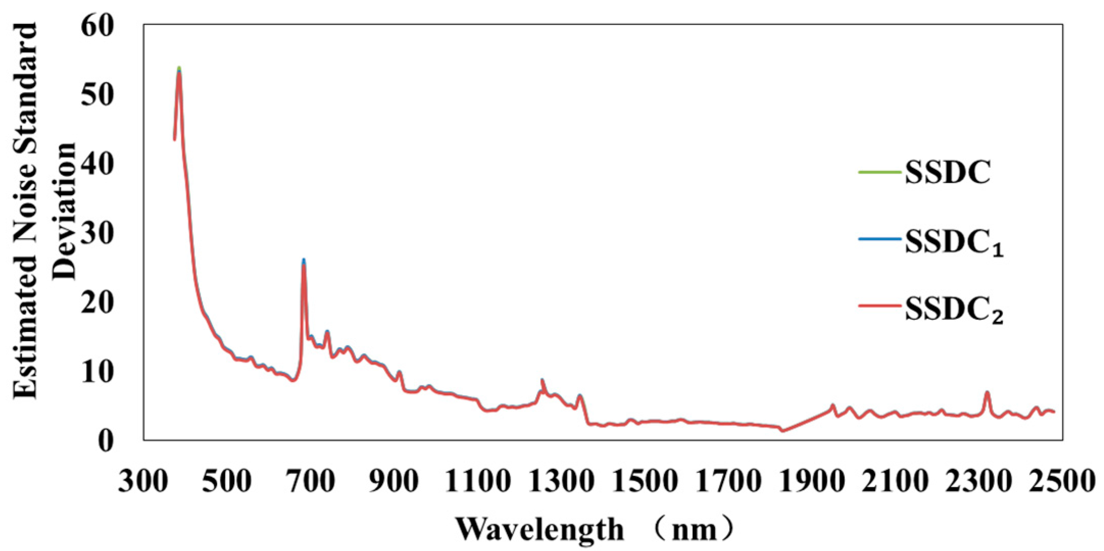
We analyze the influences of sub-block size by using hyperspectral image as shown in Figure 1a. From the experiments, we found that, when the sub-block size is 4 × 4, or 5 × 5, some sub-blocks are homogeneous and have similar DN values in certain bands; thus, it makes the matrix inversion in multiple linear regression infeasible. When the sub-block size is too large, such as 15 × 15 and 30 × 30, some sub-blocks contain multiple types of earth surface features, and the results of noise estimation become inaccurate and instable. When the sub-block size is 6 × 6, as shown in Figure 2 and Figure 3, the results of noise estimation are reliable and stable. Therefore, we set the sub-block size to 6 × 6 for SSDC, SSDC1 and SSDC2. The width and height of each sub-block are set as = 6, = 6.
2.2. Kernelization and Regularization
After noise is estimated through SSDC, SSDC1 or SSDC2, it will be included in KMNF. In KMNF, in order to get the new components ordered by image quality after dimensionality reduction, we should minimize the . For the convenience of mathematics, we can maximize the , which can be presented as
For the kernelization of , we will consider an embedding map
where , , , and nonlinear mapping can transform the original data into higher dimensional feature space [34].
After mapping , the kernelized can be expressed as
Traditionally, the inner products () sometimes can be computed more efficiently as a direct function of the input features, without explicitly computing the mapping [34]. This function is called the kernel function , which can be expressed as
Therefore, Equation (25) could be written as
where with elements , and with elements . To ensure the uniqueness of the result in Equation (27), we regulate the by introducing a regulator , similarly to what the other kernel methods (e.g., KMNF, KPCA [28,31]) have done. This way, we get a version which is regulated as
2.3. OKMNF Transformation
The regulated version described above is a symmetric generalized eigenvalue problem, which could be solved by maximizing the Rayleigh quotient in Equation (28). Therefore, this problem can be written as
where and are eigenvalues and eigenvectors of , respectively. , after mapping , transforms to . Thus, we can get the value of b, and the feature extraction result can be obtained by:
From the above analysis, we can see that noise estimation is a very critical step in the OKMNF method. Firstly, in the original data space, based on original hyperspectral data , we get the estimated data calculated by multiple linear regression models. Then, we transform the original real hyperspectral data and the estimated data to the kernel space. In this space, we get the results of noise estimation through calculating the difference of kernel and kernel . It means that the noise is estimated in the kernel space. Finally, we get the transformation matrix by maximizing regulated and achieve the dimensionality reduction. A good noise estimation is important for effective dimensionality reduction.
In many real applications, a hyperspectral image typically has a huge amount of pixels. Then, the kernel matrix could be very large (for example, the matrix sizes of and are by , and is the number of pixels). In this case, even in conventional hyperspectral remote sensing images, the kernel matrix will exceed the memory capacity of an ordinary personal computer. For example, a hyperspectral image of n = 512 × 512 pixels, the size of the kernel matrix is n × n = (512 × 512) × (512 × 512) elements. To reduce memory cost and computational complexity, we can randomly subsample the image and perform the kernel eigenvalue analysis only on these selected samples (suppose m), which can be used as training samples. We can generate a transformed version of the entire image by mapping all pixels onto the primal eigenvectors obtained from the subset samples. The procedure of OKMNF is summarized in Algorithm 2.
| Algorithm 2. The Proposed OKMNF. |
| Input: hyperspectral image , and m training samples. Step 1: compute the residuals (noises) of training samples: . Step 2: dual transformation, kernelization and regularization of using Equation (22). Step 3: compute the eigenvectors of . Step 4: mapping all pixels onto the primal eigenvectors. Output: feature extraction result . |
3. Experiments and Results
This section designs three experiments to evaluate the performances of a few noise estimation algorithms and dimensionality reduction methods. The first experiment using real images with different land covers is to assess the robustness of noise estimation algorithms adopted in OKMNF, and the results are shown in Figure 4. The other two experiments are to validate the performances of dimensionality reduction methods in terms of maximum likelihood-based classification (ML) on two real hyperspectral images. The experimental results of Indian Pines image (as shown in Figure 5) are shown in Figure 6, Figure 7, Figure 8 and Figure 9. The experimental results of Minamimaki scene image (as shown in Figure 10) are shown in Figure 11, Figure 12 and Figure 13.
3.1. Parameter Tuning
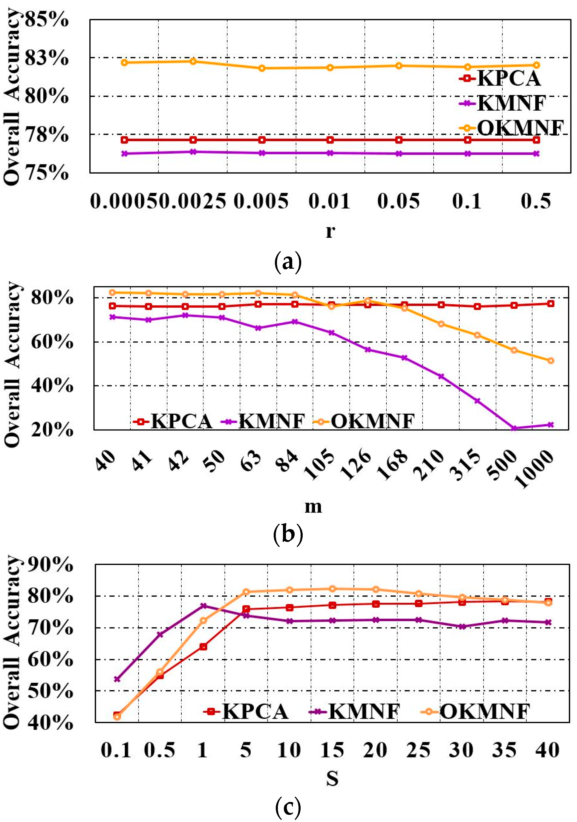
In Equation (28), we introduced a parameter to guarantee the uniqueness of the eigenvectors. Figure 7a and Figure 12a show the sensitivity of kernel dimensionality reduction methods (KPCA, KMNF, and OKMNF) with respect to . We can see that the values of parameter have little effect on kernel dimensionality reduction methods, and OKMNF gets overall better or comparable accuracy than KMNF and KPCA. To fairly compare different dimensionality reduction methods, we adopt the optimal value of parameter within the range of requirements when the classification accuracy of hyperspectral images achieves the maximum value. According to our empirical study, in the Indian Pines scene, of OKMNF, KMNF, and KPCA are all set to 0.0025, and in the Minamimaki Scene, of KMNF is set to 0.1, and of OKMNF and KPCA are both set to 0.005.
Another important parameter is the number of subsamples (pixels), . They were used to derive eigenvectors for data transformation. Figure 7b and Figure 12b show the sensitivity of kernel dimensionality reduction methods (KPCA, KMNF, and OKMNF) with respect to . We can see that the values of parameter have little effect on KPCA. To the Indian Pines scene and the Minamimaki scene, the classification accuracy of OKMNF and KMNF both evidently descend when the value of parameter is greater than 100. However, OKMNF shows lower sensitivity on parameter than KMNF, and is even better or comparable to KPCA when the value of parameter is less than 80. We fix the number of the extracted features to see the impact of subsample size on classification. We see the performance decrease, as the number of subsample increases. The reason is that when increases, more extracted features are required. To reduce the computational time and memory use, we will adopt a small number of subsamples. It is an important empirical rule that can be considered in the applications of OKMNF. Here, we also adopt the optimal value of parameter within the range of requirements when the classification accuracy of hyperspectral images achieves the maximum value. According to our empirical study, in the Indian Pines scene, of OKMNF and KPCA are both set to 63, and of KMNF is set to 42. In the Minamimaki Scene, of KMNF and KPCA are both set to 30, and of OKMNF is set to 25.
In this paper, the employed kernel function is the Gaussian radial basis function, which is the same as KPCA, KMNF, and OKMNF [59] The Gaussian radial basis function is defined as
where and are vectors of observations, , is the mean distance between the observations in feature space and is a scale factor [33,37]. Figure 7c and Figure 12c show the sensitivity of KPCA, KMNF, and OKMNF with respect to . We can see that both OKMNF and KPCA show better performance than KMNF. In the Indian Pines scene, OKMNF performs better than KPCA. Just like above, we adopt the optimal value of parameter within the range of requirements when the classification accuracy of hyperspectral images achieves the maximum value. According to our empirical study, of KPCA, KMNF, and OKMNF are set to 35, 1, and 15 for the Indian Pines scene, respectively. Then, for the Minamimaki scene, of OKMNF is set to 25, and of KPCA and KMNF are both set to 10.
3.2. Experiments on Noise Estimation Algorithms in KMNF and OKMNF
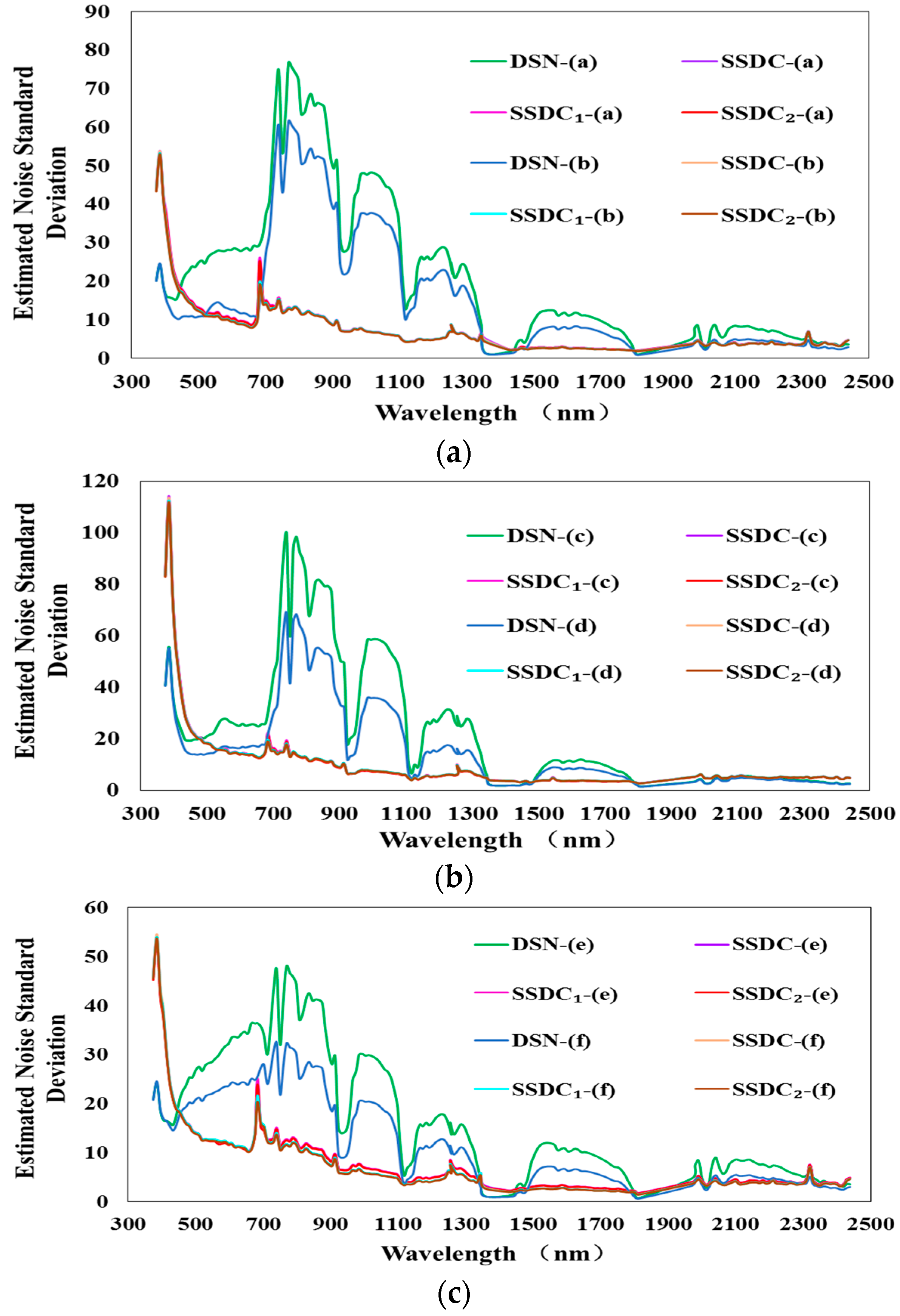
To assess the performance of noise estimation algorithms adopted in KMNF and OKMNF, six real Airborne Visible/Infrared Imaging Spectrometer (AVIRIS) radiance images with very different land cover types were used in this experiment. These images are shown in Figure 1. Each of them contains 300 × 300 pixels, and covers spectral wavelengths from 400 nm to 2500 nm. Normally, the random noise in AVIRIS sensor images is mainly additive and uncorrelated with the signal [60]. More detailed descriptions are shown in Table 1.
We assess the performance of noise estimation algorithms by computing noise standard deviation, after we get noise data through Algorithm 1. The local standard deviation (LSD) of each sub-block is estimated by
where means that four parameters are used in the multiple linear regression model and that the degree of freedom is . The LSD of each sub-block is calculated as the noise estimate of that region. The mean value of these LSD is considered as the best estimate of the band noise.
3.3. Experiments on Dimensionality Reduction Methods
In these experiments, the dimensionality reduction performance of OKMNF is evaluated in terms of classification results on two real hyperspectral images. Classification accuracies using the features extracted by PCA, KPCA, MNF, KMNF, OMNF, and OKMNF (OKMNF-SSDC, OKMNF-SSDC1, and OKMNF-SSDC2) are compared. Each experiment was run ten times, and the average of these ten experiments was reported for comparisons.
3.3.1. Experiments on the Indian Pines Image
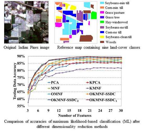
The experimental dataset was collected by the AVIRIS at Indian Pines. The image contains 145 × 145 pixels with spatial resolution of 20 m, and is with 220 spectral bands from 400 nm to 2500 nm. In this experiment, we compare with different dimensionality reduction methods based on original image including all the 220 bands. It is worth observing that 20 bands covering the region of water absorption are really noisy, thus allowing us to analyze the robustness of the different dimensionality reduction methods to real noise. As shown in Figure 5 and Figure 9, large classes are considered in this experiment. In addition, 25% of samples are randomly selected for training and the others 75% are employed for testing [61,62]. The numbers of training and testing samples are listed in Table 2. The first three features extracted by different dimensionality reduction methods are shown in Figure 8. The overall accuracies of ML classification after different dimensionality reduction methods are shown in Table 3 and Figure 6. The results of ML classification after different dimensionality reduction (number of features = 5) methods are shown in Figure 9.
3.3.2. Experiments on the Minamimaki Scene
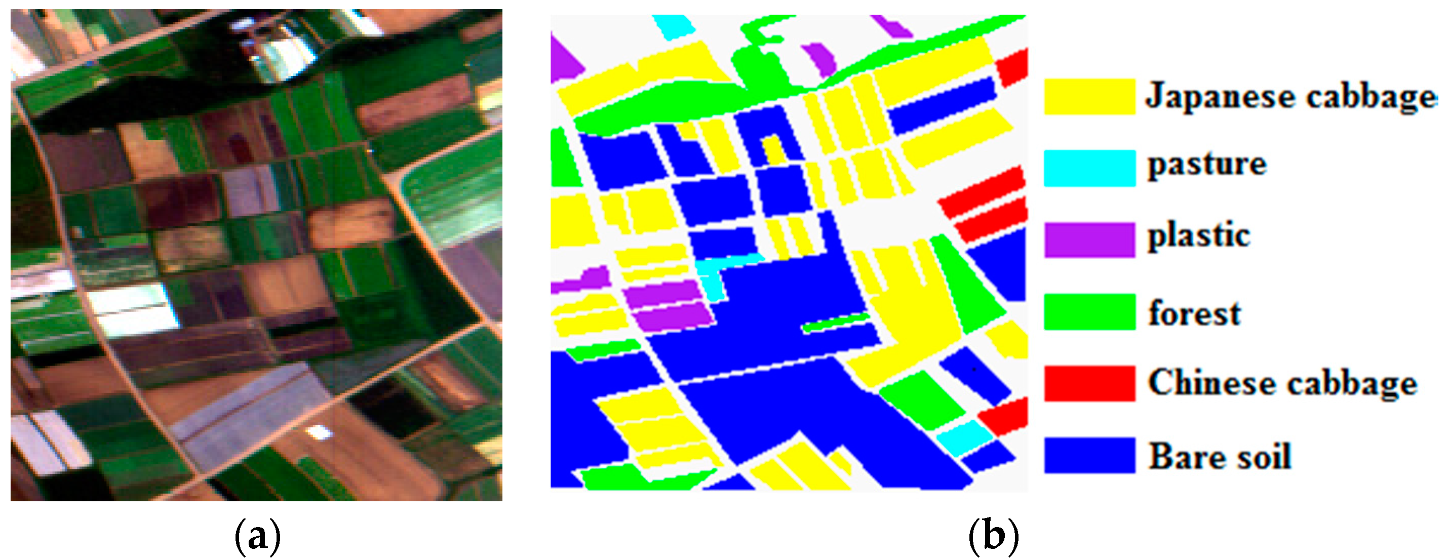
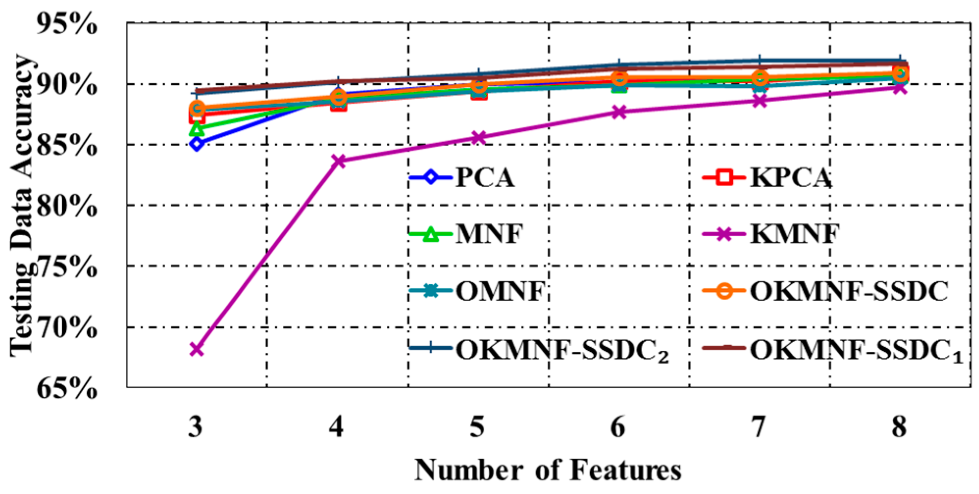
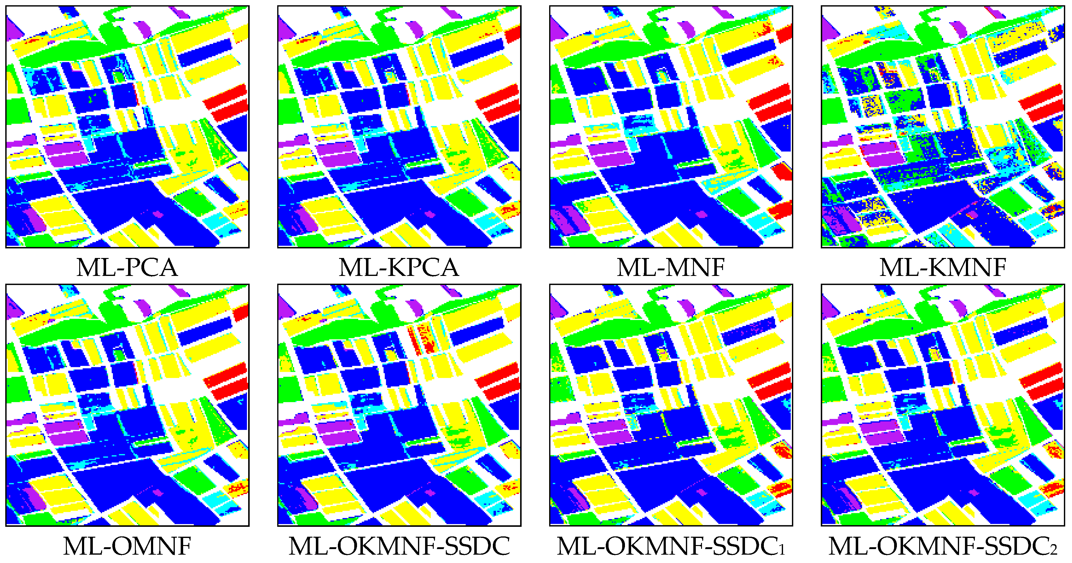
This scene was collected by the Pushbroom Hyperspectral Imager (PHI) sensor over Minamimaki, Japan. The PHI sensor was developed by the Shanghai Institute of Technical Physics of the Chinese Academy of Sciences, China. The data has 200 × 200 pixels with a spatial resolution of 3 m and 80 spectral bands from 400 nm to 850 nm. As shown in Figure 10, this image has six classes. About 10% of samples per class were randomly selected for training and the other 90% were employed for testing. The numbers of training and testing samples are listed in Table 4. The overall accuracies of ML classification after different dimensionality reduction methods are shown in Table 5 and Figure 11. The results of ML classification (number of features = 3) are shown in Figure 13.
4. Discussion
This section discusses the performances of noise estimation algorithms, and these results are shown in Section 3.2. In addition, the results of the dimensionality reduction methods are shown in Section 3.3.
Based on the experiment of assessing the performance of noise estimation algorithms adopted in KMNF and OKMNF, it can be seen in Figure 4 that the estimated noise curves through the difference of spatial neighborhood used in KMNF show a strong relationship with land cover types in the scene, and the noise levels are not the same for the two subimages from the same image. There are no such problems when the noise is estimated by OKMNF through SSDC, SSDC1 and SSDC2. We can see that SSDC, SSDC1 and SSDC2 are more reliable noise estimation methods than that used in KMNF. Thus, we can adopt SSDC, SSDC1 and SSDC2 to estimate noise for OKMNF.
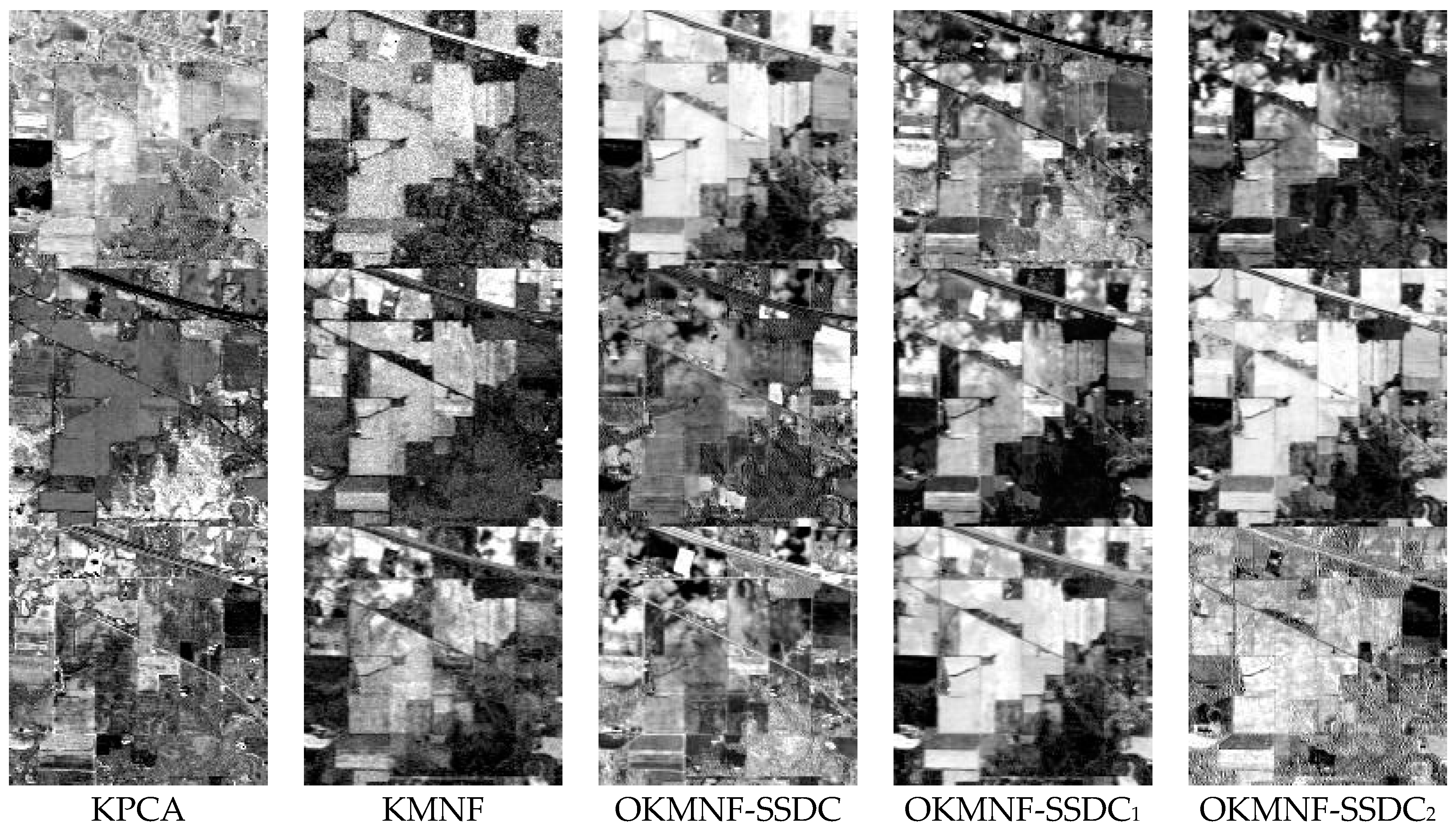
Based on the experiment of assessing the performance of dimensionality reduction methods from Section 3.3.1, it can be seen in Figure 8 that the feature quality of KMNF is worse than other dimensionality reduction methods. OKMNF, by considering SSDC, SSDC1 or SSDC2 for noise estimation, outperforms the other dimensionality reduction methods. It can be seen in Table 3, and Figure 6 and Figure 9 that the classification results using transformed data by MNF are not always better than those of PCA on low dimension space. KMNF performs worse than KPCA. By considering the spectral and spatial de-correlation for noise estimation, linear OMNF always performs better than PCA and mostly better than MNF. OKMNF, by considering SSDC, SSDC1 or SSDC2 for noise estimation, outperforms the other dimensionality reduction methods (including linear OMNF and kernel MNF), with less sensitivity for parameter settings, as well as better performances for classification. This is because OKMNF not only can treat nonlinear characteristics well within the data but also take into account both spectral and spatial correlations for reliable noise estimation. Moreover, OKMNF-SSDC1 and OKMNF-SSDC2 perform better than OKMNF-SSDC. This indicates that, by incorporating more spatial neighbors, we enable better noise estimation, as well as improve the classification performances.
Based on the experiment of assessing the performance of dimensionality reduction methods from Section 3.3.2, it can be seen in Table 5, and Figure 11 and Figure 13 that the performances of PCA, KPCA, MNF, and OMNF are very similar, and all of them are better than KMNF. When we optimized the KMNF method through SSDC, SSDC1 and SSDC2 noise estimation, the performance of KMNF was greatly improved. OKMNF gets much better results than KMNF, and also performs slightly better than the other four dimensionality reduction methods.
The two experimental results, based on the experiment of assessing the performance of dimensionality reduction methods, show that: (1) the greater the number of features extracted, the higher classification accuracy is; (2) it is better not to use KMNF for dimensionality reduction in many cases, the overall accuracies of ML classification after KMNF are lower than MNF and other dimensionality reduction methods; (3) our proposed OKMNF, OKMNF-SSDC, OKMNF-SSDC1, and OKMNF-SSDC2 perform much better than KMNF and mostly better than OMNF and MNF. These results imply that the dimensionality reduction results of KMNF are not suitable for image classification. By exploiting both spectral and spatial information for noise estimation, the proposed OKMNF benefits both dimensionality reduction and its post applications (e.g., classification). Compared to linear MNF, the proposed OKMNF not only has good performance in dimensionality reduction for classification but also does better in dealing with nonlinear problems.
To compare the efficiency of feature extraction methods, we took Indian Pines data as an example, and the consumed time (by extracting 30 features) of OKMNF-SSDC, OKMNF-SSDC1, OKMNF-SSDC2, KPCA, KMNF, OMNF, MNF, and PCA are 23.07 s, 25.27 s, 22.80 s, 1.03 s, 1.26 s, 22.87 s, 0.52 s and 0.20 s, respectively. We can find that the proposed OKMNF (OKMNF-SSDC, OKMNF-SSDC1, OKMNF-SSDC2) methods consume comparatively longer time but with better dimensionality reduction performances. However, we can use high performance computing techniques such as graphics processing unit to reduce the processing time of OKMNF. In real applications, the number of features kept for classification should be determined for both classification performance and computing cost. Too few features may not provide adequate class separability. On the other hand, more features might not always bring higher classification accuracy, which can be seen from the results listed in Table 3. It is important to use as few features as possible to avoid overfitting and minimise computational load.
5. Conclusions
This paper proposes an optimized KMNF for dimensionality reduction of hyperspectral imagery. The main reason affecting the original KMNF in dimensionality reduction is the larger error and the instability in estimating noise. Here, we conduct a comparative study for noise estimation algorithms using real images with different land cover types. The experimental results show that the combined spatial and spectral correlation information provides better results than the algorithms only using spatial neighborhood information. OKMNF adopts SSDC, SSDC1, and SSDC2 to stably estimate noise from hyperspectral images. Through this optimization, the overall accuracies of ML classification after OKMNF are much higher than those of KMNF, and the dimensionality reduction results of OKMNF are also better than OMNF, MNF, KPCA, and PCA in most situations. It can be concluded that OKMNF solves the problems existing in original KMNF well and improves the quality of dimensionality reduction. Moreover, OKMNF is valuable to reduce the dimensionality of nonlinear data. We can also expect that OKMNF will enhance the separability among endmember classes and improve the quality of spectral unmixing. Our future work will focus on incorporating more validations on other applications (e.g., target detection).
Acknowledgments
This research was supported by the National Natural Science Foundation of China under Grant No. 41571349, No. 91638201 and No. 41325004.
Author Contributions
Lianru Gao contributed to design the theoretical framework for the proposed methods and to the experimental analysis. Bin Zhao was primarily responsible for mathematical modeling and experimental design. Xiuping Jia improved the mathematical model and revised the paper. Wenzhi Liao provided important suggestions for improving technical quality of the paper. Bing Zhang proposed the original idea of the paper.
Conflicts of Interest
The authors declare no conflict of interest.
References
- Goetz, A.F.H. Three decades of hyperspectral remote sensing of the Earth: A personal view. Remote Sens. Environ. 2009, 113, S5–S16. [Google Scholar] [CrossRef]
- Plaza, A.; Benediktsson, J.A.; Boardman, J.W.; Brazile, J.; Bruzzone, L.; Camps-Valls, G.; Chanussot, J.; Fauvel, M.; Gamba, P.; Gualtieri, A.; et al. Recent advances in techniques for hyperspectral image processing. Remote Sens. Environ. 2009, 113, S110–S122. [Google Scholar] [CrossRef]
- Hughes, G. On the mean accuracy of statistical pattern recognizers. IEEE Trans. Inf. Theory 1968, 14, 55–63. [Google Scholar] [CrossRef]
- Liu, C.H.; Zhou, J.; Liang, J.; Qian, Y.T.; Li, H.X.; Gao, Y.S. Exploring structural consistency in graph regularized joint spectral-spatial sparse coding for hyperspectral image classification. IEEE J. Sel. Top. Appl. Earth Obs. Remote Sens. 2016, 99, 1–14. [Google Scholar] [CrossRef]
- Jia, X.P.; Kuo, B.; Crawford, M.M. Feature mining for hyperspectral image classification. Proc. IEEE 2013, 101, 676–697. [Google Scholar]
- Benediktsson, J.A.; Palmason, J.A.; Sveinsson, J.R. Classification of hyperspectral data from urban areas based on extended morphological profiles. IEEE Trans. Geosci. Remote Sens. 2005, 43, 480–491. [Google Scholar] [CrossRef]
- Qian, Y.T.; Yao, F.T.; Jia, S. Band selection for hyperspectral imagery using affinity propagation. IET Comput. Vis. 2010, 3, 213–222. [Google Scholar] [CrossRef]
- Falco, N.; Benediktsson, J.A.; Bruzzone, L. A study on the effectiveness of different independent component analysis algorithms for hyperspectral image classification. IEEE J. Sel. Top. Appl. Earth Obs. Remote Sens. 2014, 7, 2183–2199. [Google Scholar] [CrossRef]
- Zabalza, J.; Ren, J.C.; Wang, Z.; Zhao, H.M.; Marshall, S. Fast implementation of singular spectrum analysis for effective feature extraction in hyperspectral imaging. IEEE J. Sel. Top. Appl. Earth Obs. Remote Sens. 2015, 8, 2845–2853. [Google Scholar] [CrossRef]
- Xie, J.Y.; Hone, K.; Xie, W.X.; Gao, X.B.; Shi, Y.; Liu, X.H. Extending twin support vector machine classifier for multi-category classification problems. Intell. Data Anal. 2013, 17, 649–664. [Google Scholar]
- Chen, W.S.; Huang, J.; Zou, J.; Fang, B. Wavelet-face based subspace LDA method to solve small sample size problem in face recognition. Int. J. Wavelets Multiresolut. Inf. Process. 2009, 7, 199–214. [Google Scholar] [CrossRef]
- Gu, Y.F.; Feng, K. Optimized laplacian SVM with distance metric learning for hyperspectral image classification. IEEE J. Sel. Top. Appl. Earth Obs. Remote Sens. 2013, 6, 1109–1117. [Google Scholar] [CrossRef]
- Ma, A.L.; Zhong, Y.F.; Zhao, B.; Jiao, H.Z.; Zhang, L.P. Semisupervised subspace-based DNA encoding and matching classifier for hyperspectral remote sensing imagery. IEEE Trans. Geosci. Remote Sens. 2016, 54, 4402–4418. [Google Scholar] [CrossRef]
- Zhang, L.F.; Zhang, L.P.; Tao, D.C.; Huang, X. On combining multiple features for hyperspectral remote sensing image classification. IEEE Trans. Geosci. Remote Sens. 2012, 50, 879–893. [Google Scholar] [CrossRef]
- Melgani, F.; Bruzzone, L. Classification of hyperspectral remote sensing images with support vector machines. IEEE Trans. Geosci. Remote Sens. 2004, 42, 1778–1790. [Google Scholar] [CrossRef]
- Harsanyi, J.; Chang, C. Hyperspectral image classification and dimensionality reduction: An orthogonal subspace projection approach. IEEE Trans. Geosci. Remote Sens. 1994, 32, 779–785. [Google Scholar] [CrossRef]
- Wang, Q.; Lin, J.; Yuan, Y. Salient band selection for hyperspectral image classification via manifold ranking. IEEE Trans. Neural Netw. Learn. Syst. 2016, 27, 1279–1289. [Google Scholar] [CrossRef] [PubMed]
- Yuan, Y.; Lin, J.; Wang, Q. Dual clustering based hyperspectral band selection by contextual analysis. IEEE Trans. Geosci. Remote Sens. 2016, 54, 1431–1445. [Google Scholar] [CrossRef]
- Yuan, Y.; Lin, J.; Wang, Q. Hyperspectral image classification via multi-task joint sparse representation and stepwise MRF optimization. IEEE Trans. Cybern. 2016, 46, 2966–2977. [Google Scholar]
- Fukunaga, K. Introduction to Statistical Pattern Recognition; Academic Press: Cambridge, MA, USA, 1990. [Google Scholar]
- Kuo, B.C.; Landgrebe, D.A. Nonparametric weighted feature extractionfor classification. IEEE Trans. Geosci. Remote Sens. 2004, 42, 1096–1105. [Google Scholar]
- Ly, N.; Du, Q.; Fowler, J.E. Sparse graph-based discriminant analysis for hyperspectral imagery. IEEE Trans. Geosci. Remote Sens. 2014, 52, 3872–3884. [Google Scholar]
- Ly, N.; Du, Q.; Fowler, J.E. Collaborative graph-based discriminant analysis for hyperspectral imagery. IEEE J. Sel. Top. Appl. Earth Obs. Remote Sens. 2014, 7, 2688–2696. [Google Scholar] [CrossRef]
- Xue, Z.H.; Du, P.J.; Li, J.; Su, H.J. Simultaneous sparse graph embedding for hyperspectral image classification. IEEE Trans. Geosci. Remote Sens. 2015, 53, 6114–6133. [Google Scholar] [CrossRef]
- Roger, E.R. Principal components transform with simple, automatic noise adjustment. Int. J. Remote Sens. 1996, 17, 2719–2727. [Google Scholar] [CrossRef]
- Green, A.A.; Berman, M.; Switzer, P.; Craig, M.D. A transformation for ordering multispectral data in terms of image quality with implications for noise removal. IEEE Trans. Geosci. Remote Sens. 1998, 26, 65–74. [Google Scholar] [CrossRef]
- Chen, P.H.; Jiao, L.C.; Liu, F.; Gou, S.P.; Zhao, J.Q.; Zhao, Z.Q. Dimensionality reduction of hyperspectral imagery using sparse graph learning. IEEE J. Sel. Top. Appl. Earth Obs. Remote Sens. 2016, 99, 1–17. [Google Scholar] [CrossRef]
- Lee, J.B.; Woodyatt, S.; Berman, M. Enhancement of high spectral resolution remote-sensing data by a noise-adjusted principal components transform. IEEE Trans. Geosci. Remote Sens. 1990, 28, 295–304. [Google Scholar] [CrossRef]
- Bachmann, C.M.; Ainsworth, T.L.; Fusina, R.A. Exploiting manifold geometry in hyperspectral imagery. IEEE Trans. Geosci. Remote Sens. 2005, 43, 441–454. [Google Scholar]
- Mohan, A.; Sapiro, G.; Bosch, E. Spatially coherent nonlinear dimensionality reduction and segmentation of hyperspectral images. IEEE Geosci. Remote Sens. Lett. 2007, 4, 206–210. [Google Scholar] [CrossRef]
- Nielsen, A.A. Kernel maximum autocorrelation factor and minimum noise fraction transformations. IEEE Trans. Image Process. 2011, 20, 612–624. [Google Scholar] [CrossRef] [PubMed]
- Gomez-Chova, L.; Nielsen, A.A.; Camps-Valls, G. Explicit signal to noise ratio in reproducing kernel hilbert spaces. In Proceedings of the IEEE International Geoscience and Remote Sensing Symposium (IGARSS), Vancouver, BC, Canada, 24–29 July 2011; pp. 3570–3573. [Google Scholar]
- Nielsen, A.A.; Vestergaard, J.S. Parameter optimization in the regularized kernel minimum noise fraction transformation. In Proceedings of the IEEE International Geoscience and Remote Sensing Symposium (IGARSS), Munich, Germany, 22–27 July 2012; pp. 370–373. [Google Scholar]
- Shawe-Taylor, J.; Cristianini, N. Kernel Methods for Pattern Analysis; Cambridge University Press: New York, NY, USA, 2004. [Google Scholar]
- Li, W.; Prasad, S.; Fowler, J.E. Decision fusion in kernel-induced spaces for hyperspectral image classification. IEEE Trans. Geosci. Remote Sens. 2014, 52, 3399–3411. [Google Scholar] [CrossRef]
- Li, W.; Prasad, S.; Fowler, J.E.; Bruce, L.M. Locality preserving dimensionality reduction and classification for hyperspectral image analysis. IEEE Trans. Geosci. Remote Sens. 2012, 50, 1185–1198. [Google Scholar] [CrossRef]
- Li, W.; Prasad, S.; Fowler, J.E.; Bruce, L.M. Locality-preserving discriminant analysis in kernel-induced feature spaces for hyperspectral image classification. IEEE Geosci. Remote Sens. Lett. 2011, 8, 894–898. [Google Scholar] [CrossRef]
- Zhang, Y.H.; Prasad, S. Locality preserving composite kernel feature extraction for multi-source geospatial image analysis. IEEE J. Sel. Top. Appl. Earth Obs. Remote Sens. 2015, 8, 1385–1392. [Google Scholar] [CrossRef]
- Kuo, B.C.; Ho, H.H.; Li, C.H.; Huang, C.C.; Taur, J.S. A kernel-based feature selection method for SVM with RBF kernel for hyperspectral image classification. IEEE J. Sel. Top. Appl. Earth Obs. Remote Sens. 2014, 7, 317–326. [Google Scholar]
- Schölkopf, B.; Smola, A.; Müller, K.-R. Nonlinear component analysis as a kernel eigenvalue problem. Neural Comput. 1998, 10, 1299–1319. [Google Scholar] [CrossRef]
- Gao, L.R.; Zhang, B.; Chen, Z.C.; Lei, L.P. Study on the issue of noise estimation in dimension reduction of hyperspectral images. In Proceedings of the IEEE Workshop on Hyperspectral Image and Signal Processing: Evolution in Remote Sensing (WHISPERS), Lisbon, Portugal, 6–9 June 2011; pp. 1–4. [Google Scholar]
- Zhao, B.; Gao, L.R.; Zhang, B. An optimized method of kernel minimum noise fraction for dimensionality reduction of hyperspectral imagery. In Proceedings of the IEEE International Geoscience and Remote Sensing Symposium (IGARSS), Beijing, China, 10–15 July 2016; pp. 48–51. [Google Scholar]
- Zhao, B.; Gao, L.R.; Liao, W.Z.; Zhang, B. A new kernel method for hyperspectral image feature extraction. Geo-Spat. Inf. Sci. 2017, 99, 1–11. [Google Scholar]
- Bioucas-Dias, J.M.; Plaza, A.; Dobigeon, N.; Parente, M.; Du, Q.; Gader, P.; Chanussot, J. Hyperspectral unmixing overview: Geometrical, statistical, and sparse regression-based approaches. IEEE J. Sel. Top. Appl. Earth Obs. Remote Sens. 2012, 5, 354–379. [Google Scholar] [CrossRef]
- Jia, S.; Xie, Y.; Tang, G.H.; Zhu, J.S. Spatial-spectral-combined sparse representation-based classification for hyperspectral imagery. Soft Comput. 2014, 1–10. [Google Scholar] [CrossRef]
- Chen, C.; Li, W.; Tramel, E.W.; Cui, M.S.; Prasad, S.; Fowler, J.E. Spectral–spatial preprocessing using multihypothesis prediction for noise-robust hyperspectral image classification. IEEE J. Sel. Top. Appl. Earth Obs. Remote Sens. 2014, 7, 1047–1059. [Google Scholar] [CrossRef]
- Ghamisi, P.; Benediktsson, J.A.; Jon, A.; Cavallaro, G.; Plaza, A. automatic framework for spectral–spatial classification based on supervised feature extraction and morphological attribute profiles. IEEE J. Sel. Top. Appl. Earth Obs. Remote Sens. 2014, 7, 2147–2160. [Google Scholar] [CrossRef]
- Gao, L.R.; Du, Q.; Yang, W.; Zhang, B. A comparative study on noise estimation for hyperspectral imagery. In Proceedings of the IEEE Workshop on Hyperspectral Image and Signal Processing: Evolution in Remote Sensing (WHISPERS), Shanghai, China, 4–7 June2012; pp. 1–4. [Google Scholar]
- Roger, E.R.; Arnold, F.J. Reliably estimating the noise in AVIRIS hyperspectral images. Int. J. Remote Sens. 1996, 17, 1951–1962. [Google Scholar] [CrossRef]
- Gao, L.R.; Du, Q.; Zhang, B.; Yang, W.; Wu, Y.F. A comparative study on linear regression-based noise estimation for hyperspectral imagery. IEEE J. Sel. Top. Appl. Earth Obs. Remote Sens. 2013, 6, 488–498. [Google Scholar] [CrossRef]
- Gao, L.R.; Zhang, B.; Sun, X.; Li, S.S.; Du, Q.; Wu, C.S. Optimized maximum noise fraction for dimensionality reduction of Chinese HJ-1A hyperspectral data. EURASIP J. Adv. Signal Process. 2013, 1, 1–12. [Google Scholar] [CrossRef]
- Gao, L.R.; Zhang, B.; Zhang, X.; Zhang, W.J.; Tong, Q.X. A new operational method for estimating noise in hyperspectral images. IEEE Geosci. Remote Sens. Lett. 2008, 5, 83–87. [Google Scholar] [CrossRef]
- Liu, X.; Zhang, B.; Gao, L.R.; Chen, D.M. A maximum noise fraction transform with improved noise estimation for hyperspectral images. Sci. China Ser. F Inf. Sci. 2009, 52, 1578–1587. [Google Scholar] [CrossRef]
- Landgrebe, D.A.; Malaret, E. Noise in remote-sensing systems: The effect on classification error. IEEE Trans. Geosci. Remote Sens. 1986, 24, 294–299. [Google Scholar] [CrossRef]
- Corner, B.R.; Narayanan, R.M.; Reichenbach, S.E. Noise estimation in remote sensing imagery using data masking. Int. J. Remote Sens. 2003, 24, 689–702. [Google Scholar] [CrossRef]
- Gao, B.-C. An operational method for estimating signal to noise ratios from data acquired with imaging spectrometers. Remote Sens. Environ. 1993, 43, 23–33. [Google Scholar] [CrossRef]
- Documentation for Minimum Noise Fraction Transformations. Available online: http://people.compute.dtu.dk/alan/software.html (accessed on 31 March 2017).
- Wu, Y.F.; Gao, L.R.; Zhang, B.; Zhao, H.N.; Li, J. Real-time implementation of optimized maximum noise fraction transform for feature extraction of hyperspectral images. J. Appl. Remote Sens. 2014, 8, 1–16. [Google Scholar] [CrossRef]
- Camps-Valls, G.; Bruzzone, L. Kernel-based methods for hyperspectral image classification. IEEE Trans. Geosci. Remote Sens. 2005, 43, 1351–1362. [Google Scholar] [CrossRef]
- Acito, N.; Diani, M.; Corsini, G. Signal-dependent noise modeling andmodel parameter estimation in hyperspectral images. IEEE Trans. Geosci. Remote Sens. 2011, 49, 2957–2971. [Google Scholar] [CrossRef]
- Zhang, X.J.; Xu, C.; Li, M.; Sun, X.L. Sparse and low-rank coupling image segmentation model via nonconvex regularization. Int. J. Pattern Recognit. Artif. Intell. 2015, 29, 1–22. [Google Scholar] [CrossRef]
- Zhu, Z.X.; Jia, S.; He, S.; Sun, Y.W.; Ji, Z.; Shen, L.L. Three-dimensional Gabor feature extraction for hyperspectral imagery classification using a memetic framework. Inf. Sci. 2015, 298, 274–287. [Google Scholar] [CrossRef]
Figure 1.
Airborne Visible/Infrared Imaging Spectrometer radiance images used for noise estimation, where (a) is the first subimage of Jasper Ridge; (b) is the second subimage of Jasper Ridge; (c) is the first subimage of Low Altitude; (d) is the second subimage of Low Altitude; (e) is the first subimage of Moffett Field; and (f) is the second subimage of Moffett Field.
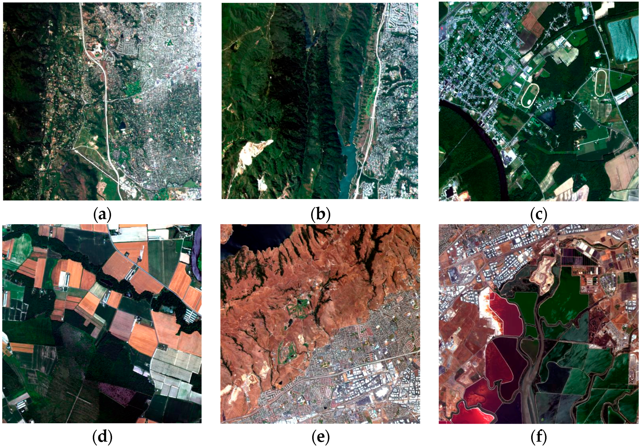
Figure 2.
Noise estimation results of spectral and spatial de-correlation (SSDC) of Figure 1a in a different size of sub-block.
Figure 2.
Noise estimation results of spectral and spatial de-correlation (SSDC) of Figure 1a in a different size of sub-block.
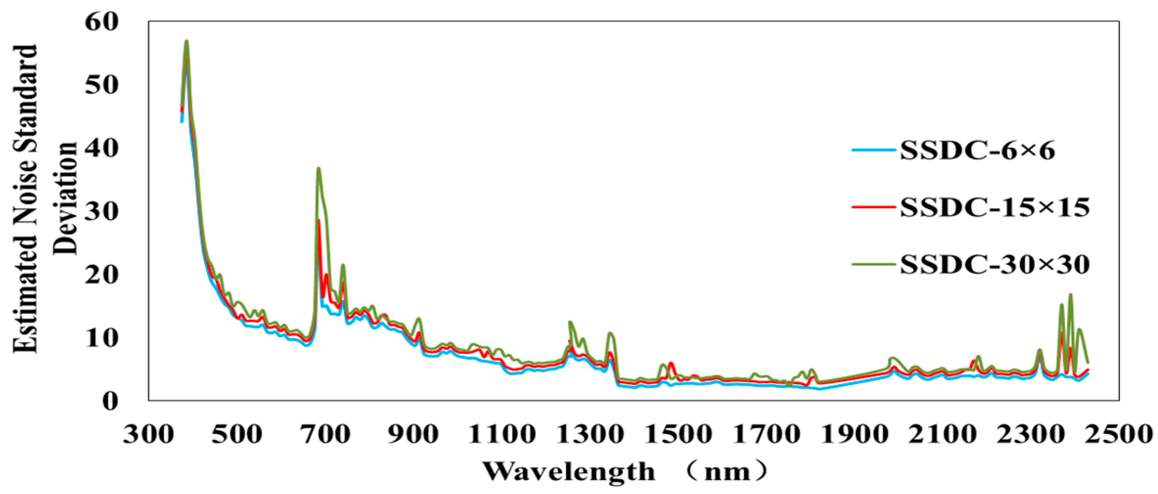
Figure 3.
Noise estimation results of SSDC, SSDC1, and SSDC2 of Figure 1a in the 6 6 size of sub-block.
Figure 3.
Noise estimation results of SSDC, SSDC1, and SSDC2 of Figure 1a in the 6 6 size of sub-block.

Figure 4.
Noise estimation results of (a) Figure 1a,b; (b) Figure 1c,d; (c) Figure 1e,f, through the difference of spatial neighborhood (DSN) used in kernel minimum noise fraction (KMNF), and the SSDC, SSDC1, and SSDC2 used in optimize KMNF (OKMNF).

Figure 5.
(a) original Indian Pines image; (b) ground reference map containing nine land-cover classes.
Figure 5.
(a) original Indian Pines image; (b) ground reference map containing nine land-cover classes.
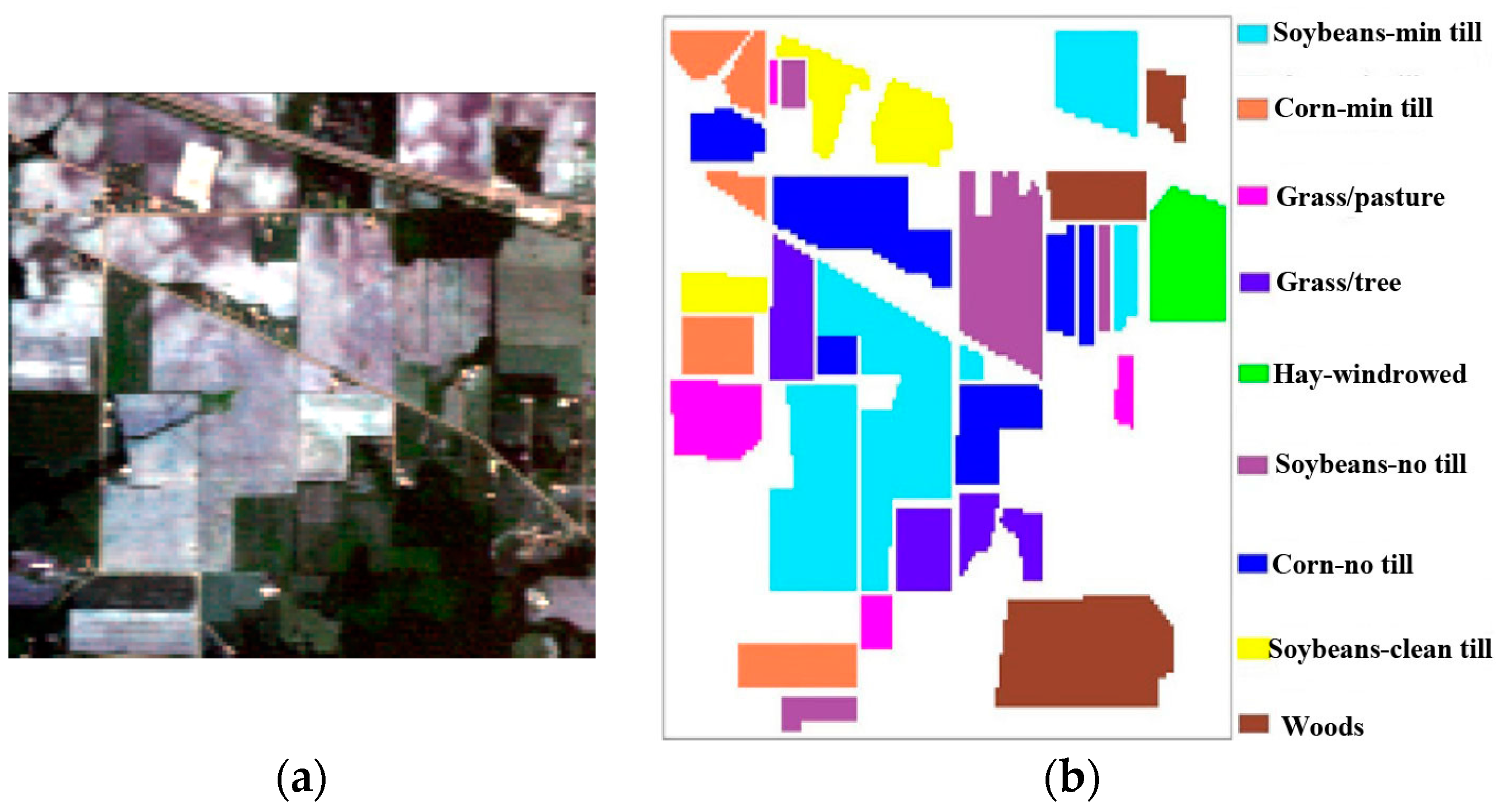
Figure 6.
Comparison of accuracies of maximum likelihood-based classification (ML) classification after different dimensionality reduction methods.
Figure 6.
Comparison of accuracies of maximum likelihood-based classification (ML) classification after different dimensionality reduction methods.
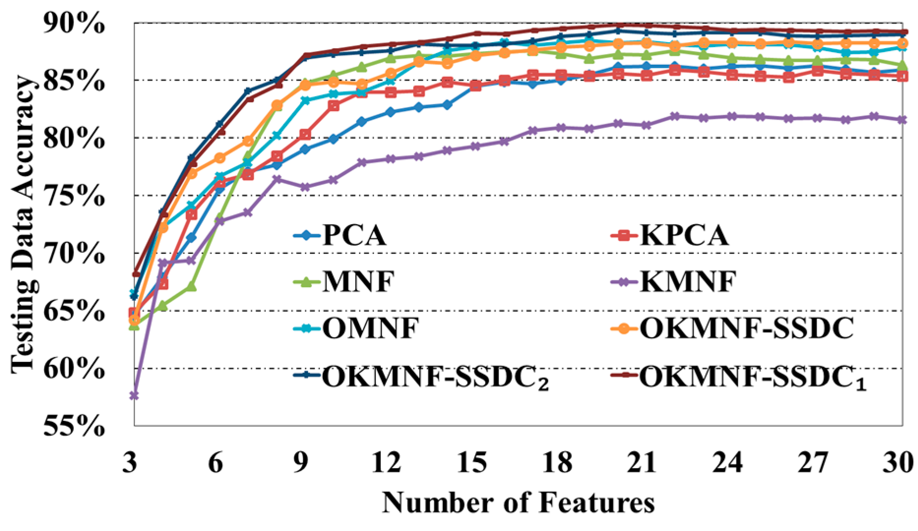
Figure 7.
Parameter tuning in the experiments using the Indian Pines dataset for ML classification after different feature extraction methods (number of features = 8), where (a) is versus accuracies; (b) is versus accuracies; (c) is versus accuracies.
Figure 7.
Parameter tuning in the experiments using the Indian Pines dataset for ML classification after different feature extraction methods (number of features = 8), where (a) is versus accuracies; (b) is versus accuracies; (c) is versus accuracies.

Figure 8.
The first three features (from up to bottom) of kernel PCA (KPCA), KMNF, OKMNF-SSDC, OKMNF-SSDC1, and OKMNF-SSDC2.
Figure 8.
The first three features (from up to bottom) of kernel PCA (KPCA), KMNF, OKMNF-SSDC, OKMNF-SSDC1, and OKMNF-SSDC2.

Figure 9.
The results of ML classification after different dimensionality reduction methods (number of features = 5).
Figure 9.
The results of ML classification after different dimensionality reduction methods (number of features = 5).
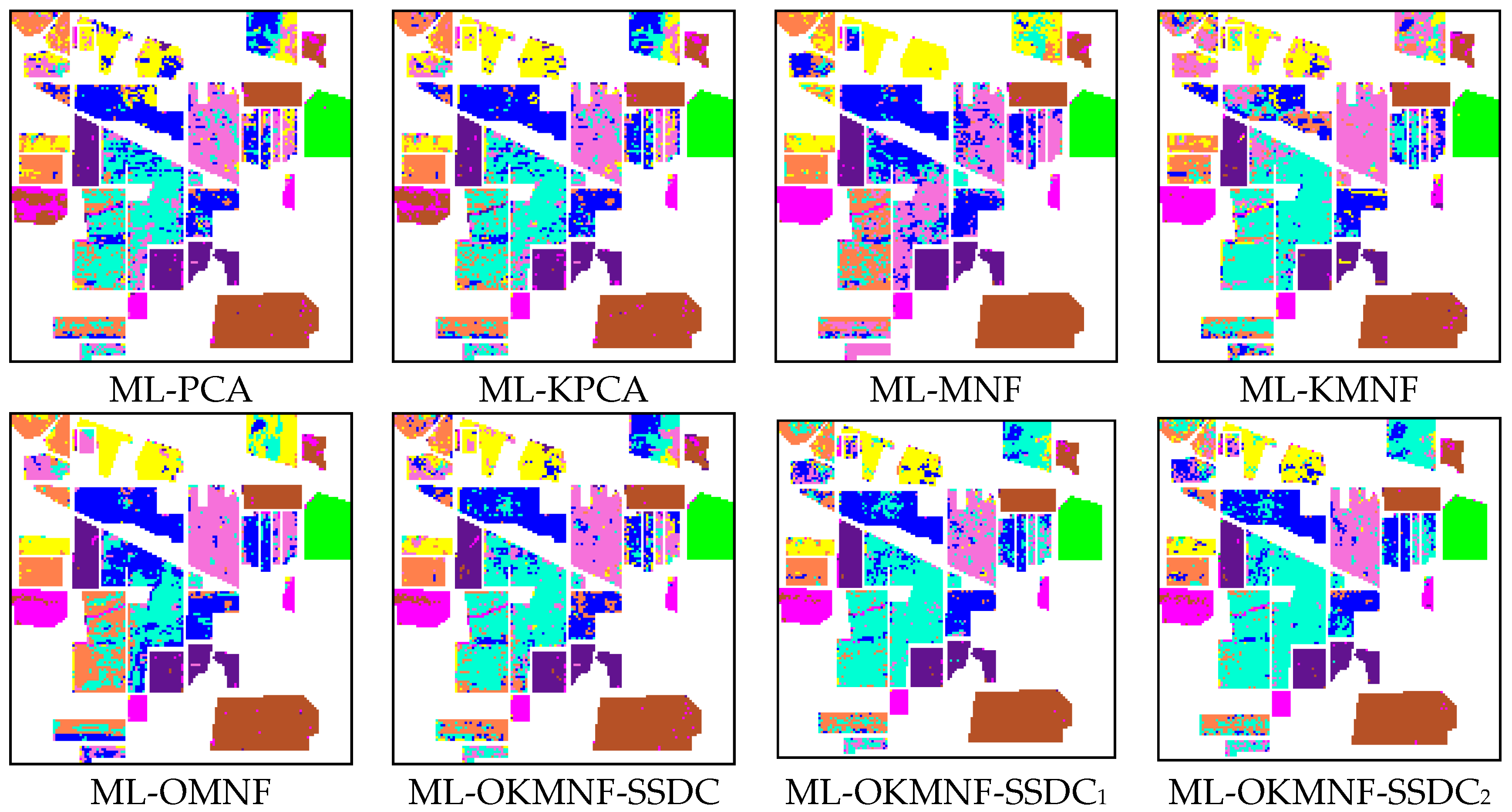
Figure 10.
(a) true color image of the Minamimaki scene; (b) ground reference map with 6 classes.

Figure 11.
Comparison of accuracies of ML classification after different dimensionality reduction methods.
Figure 11.
Comparison of accuracies of ML classification after different dimensionality reduction methods.

Figure 12.
Parameter tuning in experiments using the Minamimaki dataset for ML classification after different dimensionality methods (number of features = 8), where (a) is versus accuracies; (b) is versus accuracies; (c) is versus accuracies.
Figure 12.
Parameter tuning in experiments using the Minamimaki dataset for ML classification after different dimensionality methods (number of features = 8), where (a) is versus accuracies; (b) is versus accuracies; (c) is versus accuracies.
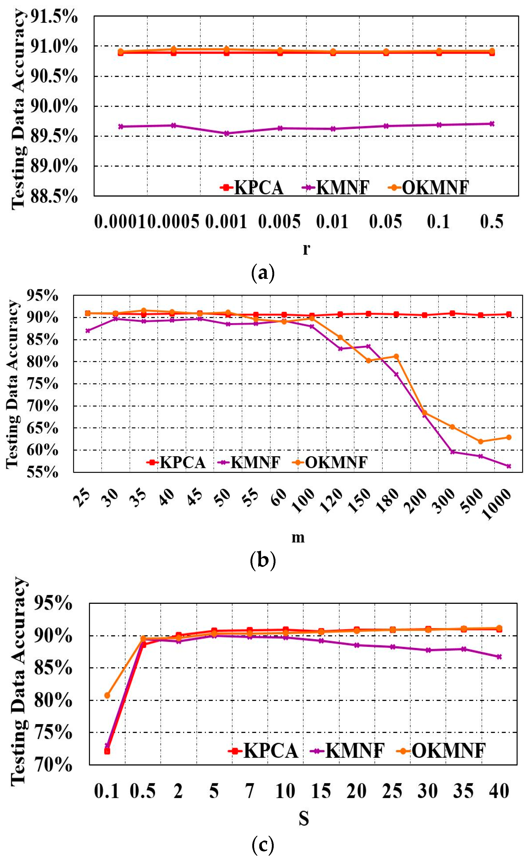
Figure 13.
The results of ML classification after different dimensionality reduction methods (number of features = 3).
Figure 13.
The results of ML classification after different dimensionality reduction methods (number of features = 3).


Table 1.
Detailed description of Airborne Visible/Infrared Imaging Spectrometer images shown in Figure 1.
Table 1.
Detailed description of Airborne Visible/Infrared Imaging Spectrometer images shown in Figure 1.
| Spatial Resolution | Acquired Site | Acquired Time | Image Description | |
|---|---|---|---|---|
| (a) | 20 m | Jasper Ridge | 3 April 1997 | Dominated by a heterogeneous city area |
| (b) | Dominated by a homogeneous vegetation area | |||
| (c) | 3.4 m | Low Altitude | 5 July 1996 | Dominated by a heterogeneous city area |
| (d) | Homogeneous farmland | |||
| (e) | 20 m | Moffett Field | 20 June 1997 | A mix of a heterogeneous city area and a homogeneous bare soil |
| (f) | Dominated by a homogeneous water |
Table 2.
Training and testing samples used in Indian Pines image.
| Classes | Training | Testing |
|---|---|---|
| Corn-no till | 359 | 1075 |
| Corn-min till | 209 | 625 |
| Grass/Pasture | 124 | 373 |
| Grass/Trees | 187 | 560 |
| Hay-windrowed | 122 | 367 |
| Soybean-no till | 242 | 726 |
| Soybean-min till | 617 | 1851 |
| Soybean-clean till | 154 | 460 |
| Woods | 324 | 970 |
| Total | 2338 | 7007 |
Table 3.
The overall accuracies of maximum likelihood-based classification (ML) classification after different dimensionality reduction methods.
Table 3.
The overall accuracies of maximum likelihood-based classification (ML) classification after different dimensionality reduction methods.
| Number of Features | PCA | KPCA | MNF | KMNF | OMNF | OKMNF-SSDC | OKMNF-SSDC1 | OKMNF-SSDC2 |
|---|---|---|---|---|---|---|---|---|
| 3 | 64.57% | 64.84% | 63.75% | 57.63% | 66.50% | 64.21% | 68.19% | 66.19% |
| 4 | 67.90% | 67.33% | 65.44% | 69.14% | 72.25% | 72.23% | 73.34% | 73.60% |
| 5 | 71.35% | 73.41% | 67.14% | 69.36% | 74.15% | 76.93% | 77.74% | 78.29% |
| 6 | 75.60% | 76.23% | 73.09% | 72.76% | 76.69% | 78.31% | 80.48% | 81.22% |
| 7 | 77.08% | 76.81% | 78.43% | 73.53% | 77.88% | 79.73% | 83.35% | 84.07% |
| 8 | 77.65% | 78.45% | 82.76% | 76.39% | 80.21% | 82.86% | 84.56% | 85.03% |
| 9 | 79.01% | 80.32% | 84.74% | 75.71% | 83.27% | 84.59% | 87.21% | 86.93% |
| 10 | 79.92% | 82.82% | 85.43% | 76.35% | 83.84% | 84.87% | 87.56% | 87.26% |
| 11 | 81.40% | 83.96% | 86.16% | 77.88% | 83.97% | 84.69% | 87.94% | 87.44% |
| 12 | 82.27% | 83.96% | 86.93% | 78.18% | 84.96% | 85.66% | 88.17% | 87.60% |
| 13 | 82.67% | 84.10% | 87.15% | 78.42% | 86.61% | 86.63% | 88.33% | 88.13% |
| 14 | 82.90% | 84.84% | 87.08% | 78.94% | 87.57% | 86.50% | 88.63% | 88.04% |
| 15 | 84.49% | 84.54% | 87.33% | 79.31% | 87.95% | 87.17% | 89.10% | 88.04% |
| 16 | 84.87% | 85.03% | 87.48% | 79.72% | 88.30% | 87.43% | 89.04% | 88.17% |
| 17 | 84.72% | 85.50% | 87.55% | 80.66% | 88.05% | 87.64% | 89.37% | 88.41% |
| 18 | 85.02% | 85.50% | 87.34% | 80.89% | 88.28% | 87.91% | 89.51% | 88.84% |
| 19 | 85.50% | 85.37% | 86.91% | 80.78% | 88.47% | 87.98% | 89.68% | 89.00% |
| 20 | 86.16% | 85.59% | 87.27% | 81.25% | 88.25% | 88.20% | 89.82% | 89.30% |
| 21 | 86.21% | 85.41% | 87.21% | 81.13% | 88.37% | 88.24% | 89.77% | 89.14% |
| 22 | 86.23% | 85.89% | 87.57% | 81.88% | 88.10% | 88.01% | 89.64% | 89.03% |
| 23 | 86.00% | 85.76% | 87.28% | 81.76% | 88.00% | 88.30% | 89.55% | 89.15% |
| 24 | 86.24% | 85.49% | 86.97% | 81.88% | 88.17% | 88.28% | 89.35% | 89.14% |
| 25 | 86.27% | 85.40% | 86.87% | 81.82% | 88.08% | 88.23% | 89.42% | 89.14% |
| 26 | 86.06% | 85.30% | 86.74% | 81.66% | 88.11% | 88.34% | 89.34% | 88.89% |
| 27 | 86.27% | 85.84% | 86.76% | 81.72% | 87.85% | 88.20% | 89.28% | 88.82% |
| 28 | 85.96% | 85.59% | 86.84% | 81.60% | 87.43% | 88.27% | 89.27% | 88.88% |
| 29 | 85.71% | 85.50% | 86.80% | 81.92% | 87.50% | 88.25% | 89.28% | 88.91% |
| 30 | 85.89% | 85.39% | 86.31% | 81.60% | 87.87% | 88.24% | 89.23% | 88.97% |
PCA: principal component analysis; KPCA: kernel PCA; MNF: minimum noise fraction; KMNF: kernel minimum noise fraction; OMNF: optimized MNF; OKMNF: optimized kernel minimum noise fraction.
Table 4.
Training and testing samples used in the Minamimaki scene.
| Classes | Training | Testing |
|---|---|---|
| Bare soil | 1238 | 11,150 |
| plastic | 33 | 300 |
| Chinese cabbage | 29 | 245 |
| forest | 111 | 1000 |
| Japanese cabbage | 425 | 3830 |
| pasture | 20 | 153 |
| Total | 1856 | 16,678 |
Table 5.
The overall accuracies of ML classification after different dimensionality reduction methods.
Table 5.
The overall accuracies of ML classification after different dimensionality reduction methods.
| Method | Number of Features | |||||
|---|---|---|---|---|---|---|
| 3 | 4 | 5 | 6 | 7 | 8 | |
| PCA | 85.14% | 89.13% | 89.86% | 90.17% | 90.44% | 90.75% |
| KPCA | 87.43% | 88.41% | 89.46% | 90.19% | 90.22% | 90.87% |
| MNF | 86.34% | 88.73% | 89.48% | 89.69% | 90.32% | 90.59% |
| KMNF | 68.30% | 83.81% | 86.02% | 87.69% | 88.61% | 89.66% |
| OMNF | 87.82% | 88.51% | 89.32% | 90.10% | 89.88% | 90.51% |
| OKMNF-SSDC | 88.10% | 88.94% | 89.98% | 90.60% | 90.63% | 90.97% |
| OKMNF-SSDC1 | 89.46% | 90.18% | 90.44% | 91.19% | 91.39% | 91.68% |
| OKMNF-SSDC2 | 89.24% | 90.17% | 90.78% | 91.56% | 91.88% | 91.89% |
© 2017 by the authors. Licensee MDPI, Basel, Switzerland. This article is an open access article distributed under the terms and conditions of the Creative Commons Attribution (CC BY) license (http://creativecommons.org/licenses/by/4.0/).
Share and Cite
MDPI and ACS Style
Gao, L.; Zhao, B.; Jia, X.; Liao, W.; Zhang, B. Optimized Kernel Minimum Noise Fraction Transformation for Hyperspectral Image Classification. Remote Sens. 2017, 9, 548. https://doi.org/10.3390/rs9060548
AMA Style
Gao L, Zhao B, Jia X, Liao W, Zhang B. Optimized Kernel Minimum Noise Fraction Transformation for Hyperspectral Image Classification. Remote Sensing. 2017; 9(6):548. https://doi.org/10.3390/rs9060548
Chicago/Turabian StyleGao, Lianru, Bin Zhao, Xiuping Jia, Wenzhi Liao, and Bing Zhang. 2017. "Optimized Kernel Minimum Noise Fraction Transformation for Hyperspectral Image Classification" Remote Sensing 9, no. 6: 548. https://doi.org/10.3390/rs9060548
Note that from the first issue of 2016, this journal uses article numbers instead of page numbers. See further details here.