UAS-Based Change Detection of the Glacial and Proglacial Transition Zone at Pasterze Glacier, Austria

Abstract

Glacier-related applications of unmanned aircraft systems (UAS) in high mountain regions with steep topography are relatively rare. This study makes a contribution to the lack of UAS applications in studying alpine glaciers in the European Alps. We transferred an established workflow of UAS-based change detection procedures to Austria’s largest glacier, the Pasterze Glacier. We focused on a selected part of the glacier tongue and its proglacial vicinity to obtain detailed knowledge of (i) the behavior of a lateral crevasse field, (ii) the evolution of glacier surface structures and velocity fields, (iii) glacier ablation behavior and the current glacier margin, and (iv) proglacial dead ice conditions and dead ice ablation. Based on two UAS flight campaigns, accomplished in 2016 (51 days apart), we produced digital elevation models (DEMs) and orthophotos with a ground sampling distance (GSD) of 0.15 m using Structure-from-Motion (SfM) photogrammetry. Electrical resistivity tomography (ERT) profiling was additionally conducted in the proglacial area. Results indicate distinct changes in the crevasse field with massive ice collapses, rapid glacier recession, surface lowering (mean of −0.9 m), and ice disintegration at the margins, calculated degree day factors on the order of −7 to −11 mm d⁻¹·°C⁻¹ for clean ice parts, and minimal changes of the debris-covered dead ice in the proglacial area. With this contribution we highlight the benefit of UAS in comparison to commonly used terrestrial methods and satellite-related approaches.

1. Introduction

Nowadays, unmanned aircraft systems (UAS) are widely used in a variety of disciplines and for a range of different purposes. There are also examples of applications of UAS in glaciology, e.g., [1]. For many reasons there is a gap between a general increasing number of UAS-related studies in the last few years [2,3] on the one hand and a more or less constant quantity of UAS used in glaciological studies on the other hand [4]. Moreover, most of these studies are not related to high mountain regions, even if there are some examples, e.g., [5]. In particular, in the European Alps only a few research-related studies are known, e.g., [6,7,8]. The glacier change was detected and mapped based on UAS, but this was not the emphasis in the latter studies. Therefore one main aim of the present study is to give an example of an application of UAS in a high alpine environment within a glaciological context.

The Pasterze Glacier (see Section 2) was investigated as a case study. This is a glacier with an extraordinarily long research history that began in 1879 [9]. Particularly the length measurements are one of the longest and most constant within the European Alps and elsewhere [10]. Apart from the length fluctuations of the glacier tongue, these annual measurements focused on parameters such as glacier surface elevation changes and the movement of the glacier surface using terrestrial methods [9,10,11]. Furthermore, photogrammetric and map-based approaches including digital elevation model (DEM) differencing gave additional insights into the glacier behavior [12,13,14,15]. Another terrestrial approach was dedicated to glacial debris cover [16]. In general, new methods are seen in addition and in respect to the long history of measurement as promising to improve the detailed knowledge of the glacier [9,13].

This study aims to obtain detailed information of (i) the behavior of a lateral crevasse field, (ii) the evolution of glacier surface structures and velocity fields, (iii) glacier ablation behavior and the current glacier margin, and (iv) proglacial dead ice conditions and possible dead ice ablation. To achieve these goals, this study follows an established procedure of UAS studies already shown for non-glaciological questions dealing with morphological changes, e.g., [17,18,19]. Proglacial dead ice conditions are investigated by electrical resistivity tomography (ERT) profiles. By using ERT it is possible to identify areas underlain by massive ice and areas influenced by permafrost [20] as shown by earlier studies in proglacial areas, e.g., [21,22]. The knowledge about proglacial buried ice conditions helps to answer the question of how possible geomorphic changes of the proglacial area are related to the changes in the sub-surface ice conditions.

This article is structured as follows: the study area and relevant previous studies are discussed in Section 2, Section 3 addresses the methods applied as well as accuracy assessment, the results obtained are presented in Section 4, followed by a discussion in Section 5 and a conclusion in Section 6.

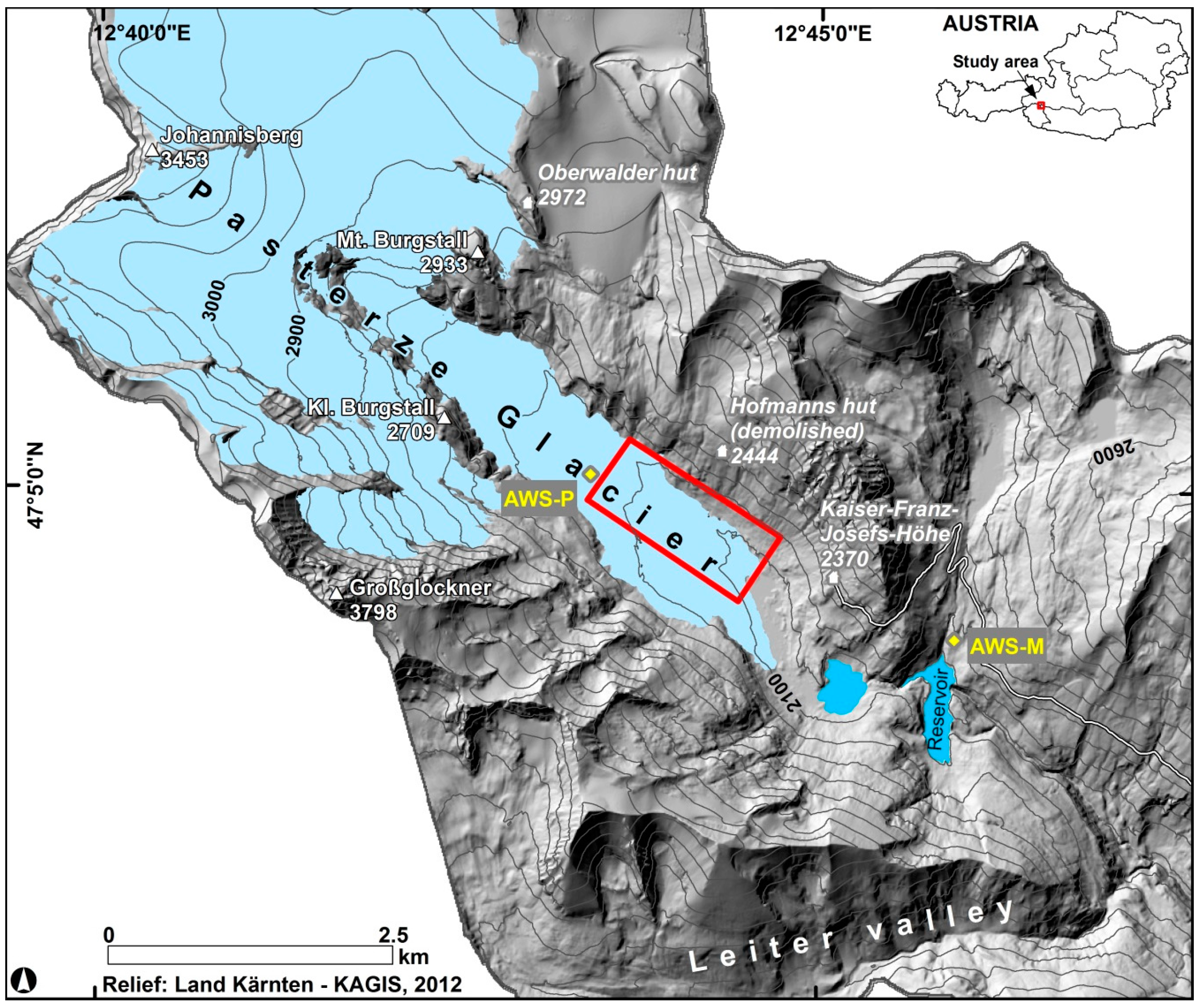
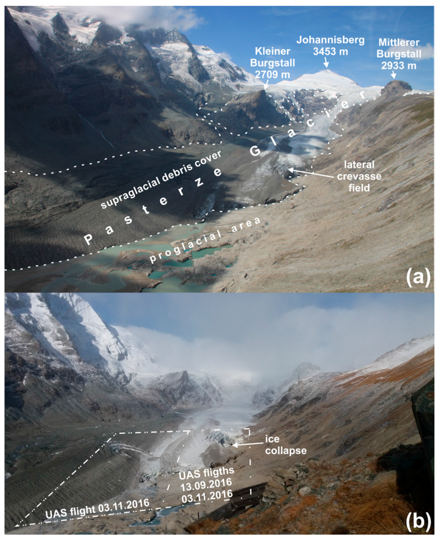
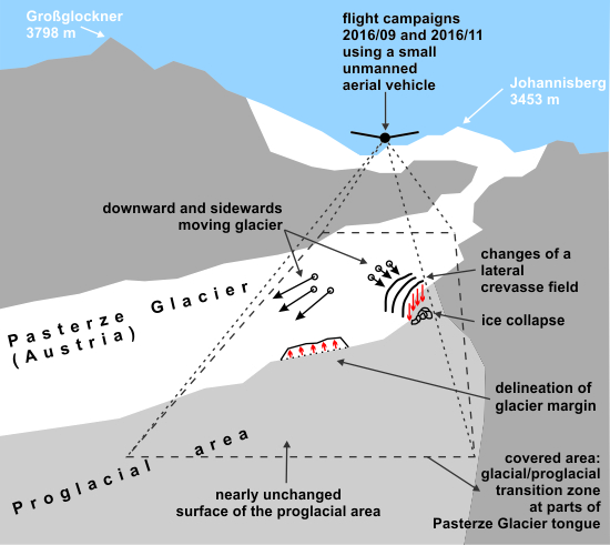
2. Study Area

The study area is located at the lower third of the glacier tongue of the Pasterze Glacier. This glacier is the largest glacier in Austria located in the Hohe Tauern Range, Austria (Figure 1). It is a compound valley glacier fed by a number of tributaries [16]. In 2012, the Pasterze Glacier had a length of 8.1 km, an areal extent of 16.6 km², and a volume of about 1.16 km³ [23]. Since the end of the Little Ice Age (LIA) in the 1850s, the glacier has been characterized by continuous recession except for a few short periods of stability and single years of minor advances [24]. The glacier did not substantially advance during the cooler and wetter periods since the 1850s related to the slow response time of the Pasterze Glacier [9].

The area investigated by the UAS-approach (see Figure 1 and Figure 2) covers an area of about 1 km². This area was fully covered by a UAS campaign in November, whereas during the September flight campaign only about half of this area was covered by the UAS-aerial photographs. This restriction is related to technical constraints during the first campaign, where it was necessary to choose an appropriate take-off and landing area (see Section 3.1.1). In the second field campaign, the time needed for setup and detailed planning was reduced and thus there was time for a second flight. Accordingly, the size of the final area being processed and discussed is 0.34 km².

3. Materials and Methods

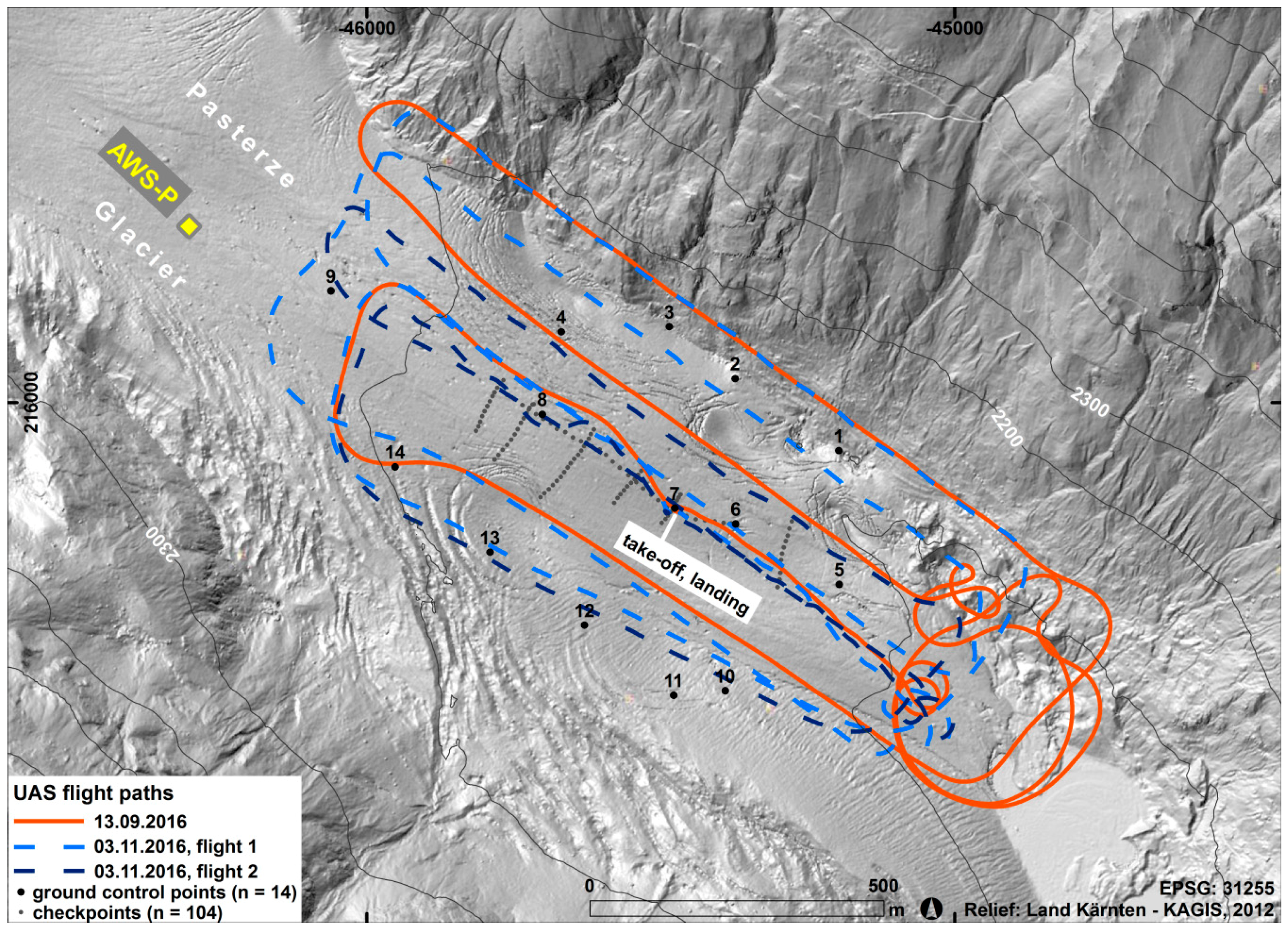
3.1. Data Acquisition

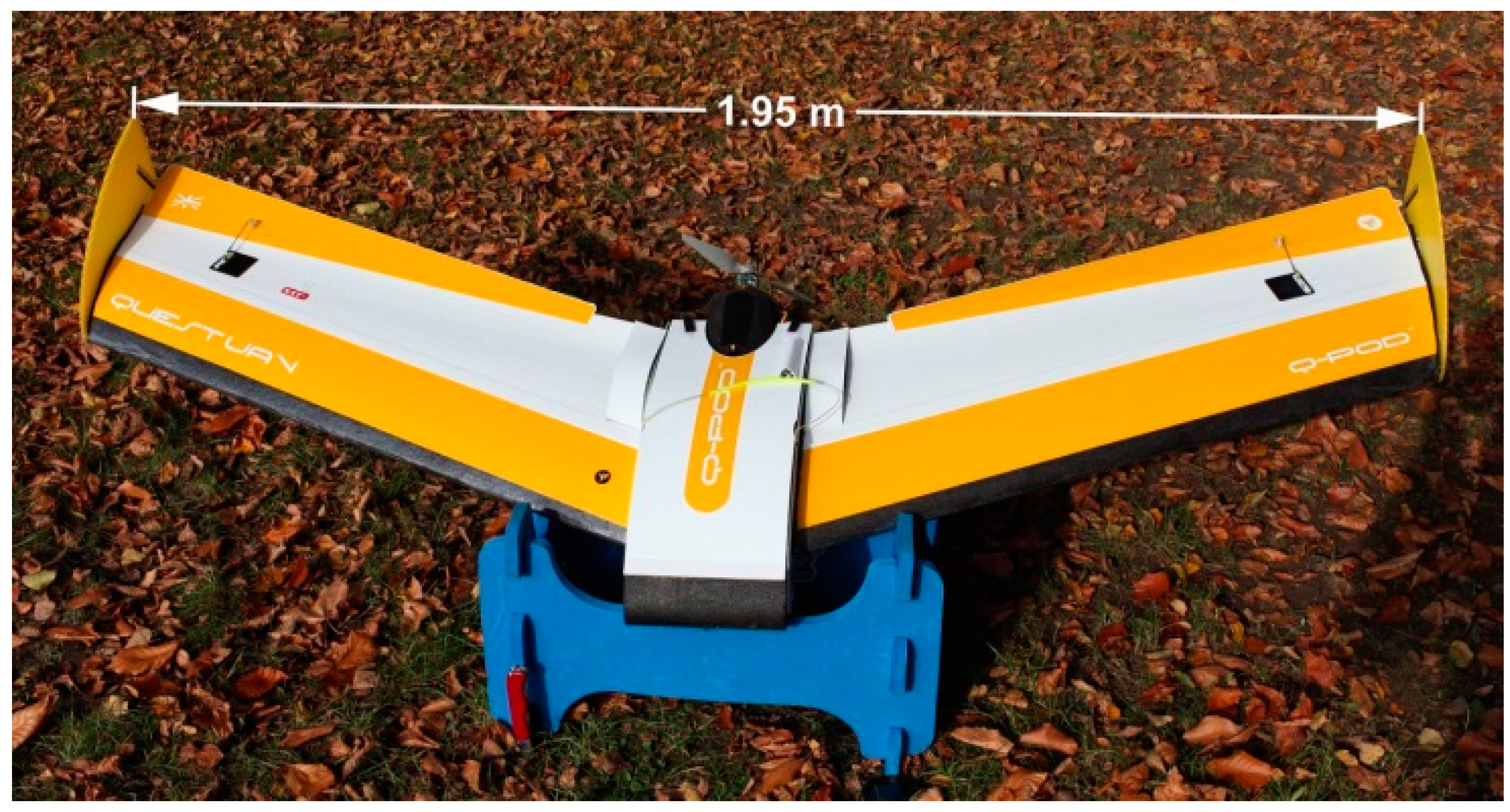
3.1.1. UAS-Based Aerial Survey

Aerial photographs were recorded using a fixed-wing UAS (see Figure 3). The flight campaigns were carried out on two days in September 2016 (13 September 2016, concerning the data in the following, also mentioned as September 2016) and November 2016 (3 November 2016, concerning the data in the following, also mentioned as November 2016). The planned image overlap was 80% (along track) and 60% (across track), and the flying height was about 150 m above ground. Figure 4 gives an overview about the flight courses. Only one flight was done in September 2016, whereas in November 2016 two flights were possible and covered nearly the full width of the glacier tongue. In September we used the UAS for the first time on a glacier and thus it took several attempts and some hours in situ to determine that the UAS had to be started windward but in an uphill direction due to the steep rock walls nearby (see Figure 2 and Figure 4). The flight time was tremendously reduced due to the wind and temperature conditions. As a consequence, the battery pack’s voltage decreased unusually fast and the flight time of around seven minutes was reduced to about three quarters compared to other study sites at lower altitude, where a flying time of at least ten minutes is usually possible. The consumer grade camera was a Sony α 6000 with an E 16 mm F2.8 lens and a resolution of 6000 × 4000 pixels. The sensor has a size of 23.5 × 15.6 mm². The number of photographs were taken as follows, both in raw file format (i.e., Sony file format Alpha Raw (ARW)) and JPEG (Joint Photographic Experts Group) file format: September 2016: 100 images, November 2016: 343 images. The shutter speed was fixed to 1/1000 s and the light sensitivity (ISO) was set to 500. The quality of the camera-based JPEG files did not seem to be suited for further processing, as mentioned in a similar discussion by [25]. For this reason and due to limitations of the software used (see Section 3.2), the ARW files were converted to JPEG using the lowest possible compression rate of the Image Data Converter software (v. 4.2.04.17270; Sony Corporation (Tokyo, Japan) 2014).

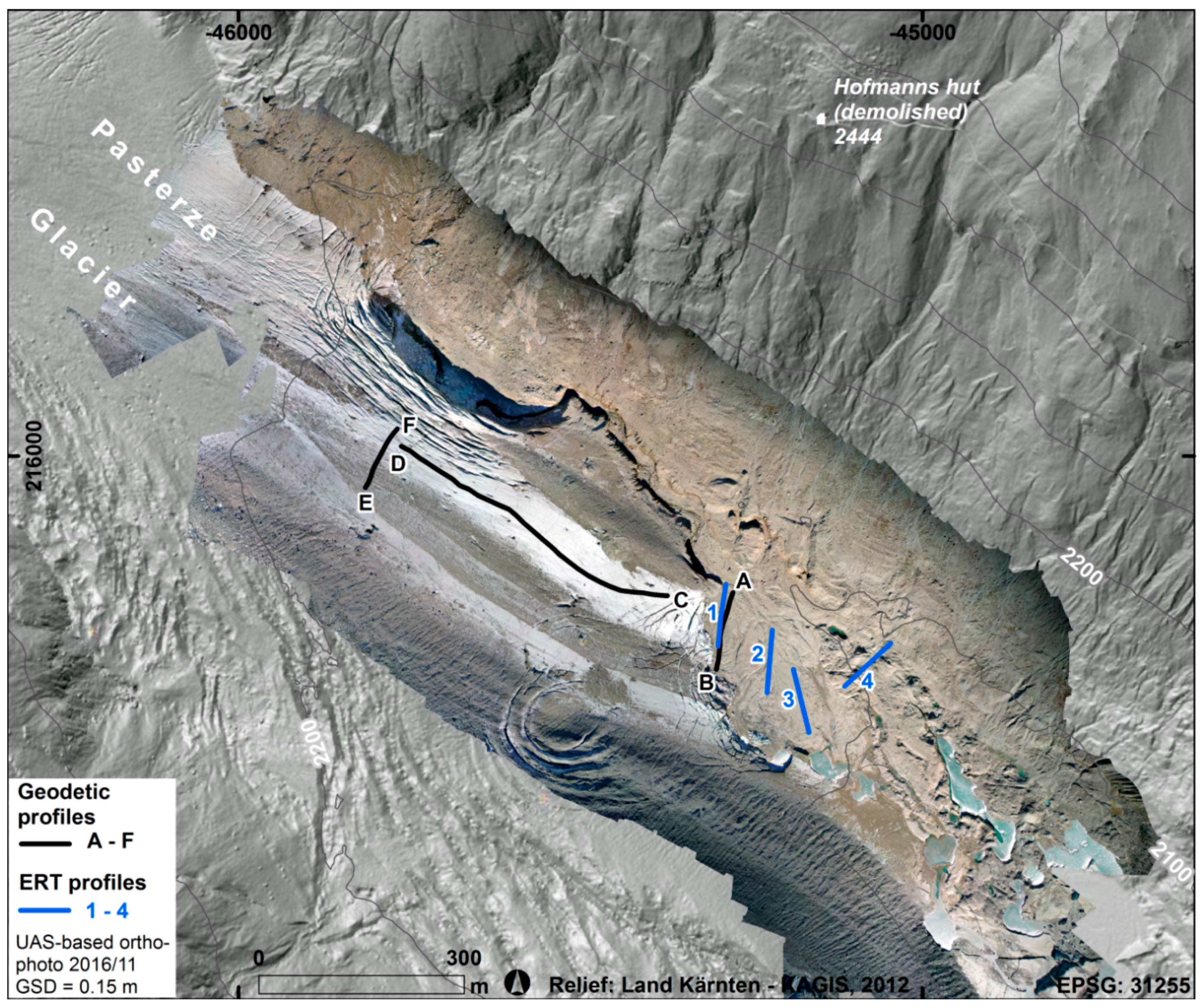
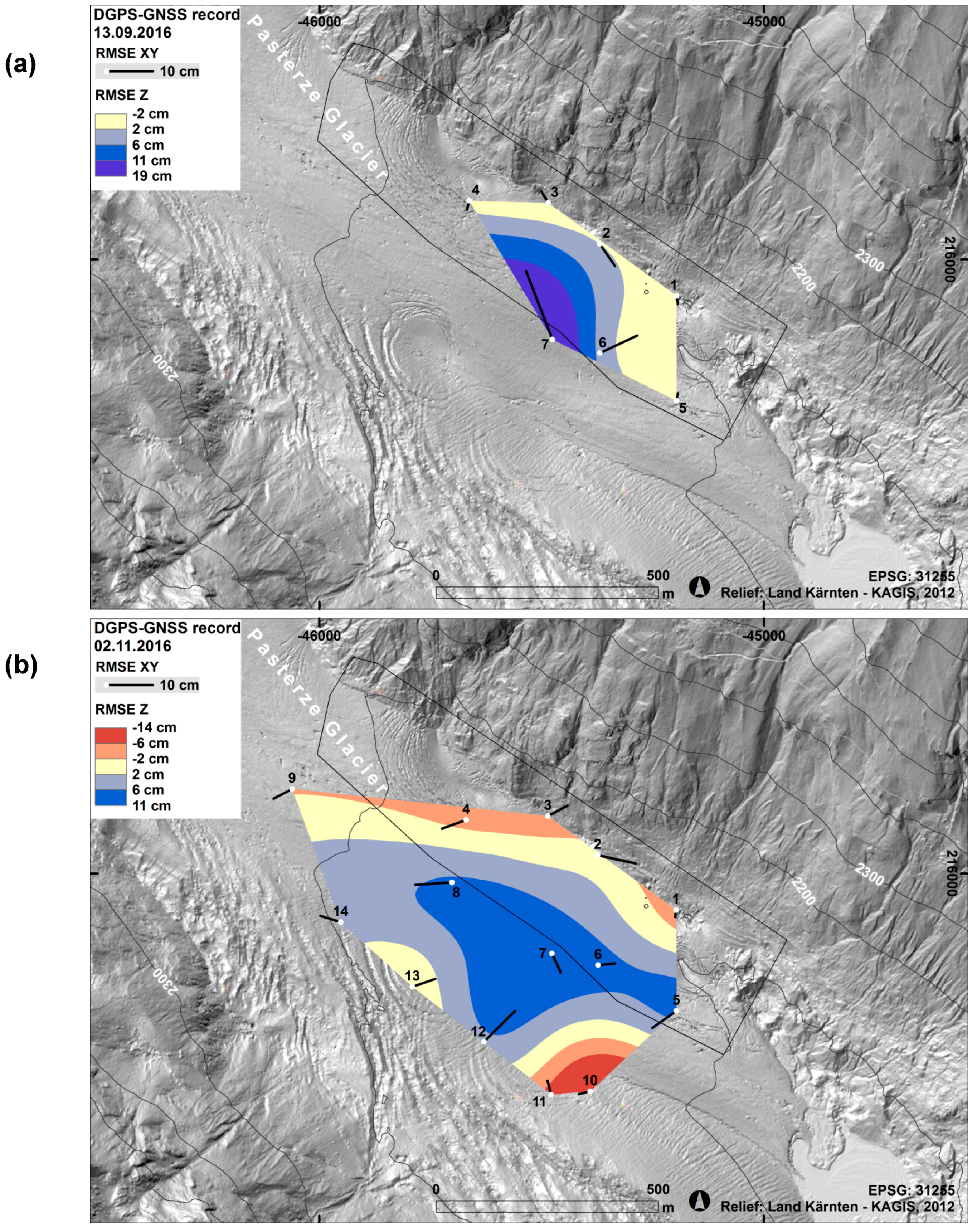
3.1.2. Geodetic Measurement

In terms of indirect georeferencing of the aerial photographs, we used ground control points (GCPs, September 2016: 7, November 2016: 14; see Figure 4 and Figure 8) visible in the photographs by using wooden target marks. The GCPs were geodetically measured with a Differential Global Positioning System (DGPS, using a Topcon HiPerV dual frequency Global Navigation Satellite System (GNSS) receiver). The measurements were done separately during both field campaigns (September 2016 and November 2016). So-called check points (see Section 3.3.1, Figure 4) were recorded in the same way only on 3 November 2016, the same day the UAS flights were made.

3.1.3. Electrical Resistivity Tomography

Electrical resistivity tomography (ERT) profiling was carried out at four profiles in the proglacial area of the Pasterze Glacier (Figure 5) using the GeoTom-2D system (Geolog2000, Starnberg, Germany). All four profiles were measured on 13 September 2016 with profile lengths of 96 m, 25 electrodes, and 4 m electrode spacing. Global Positioning System (GPS) was used to measure the starting, center, and final points of the profiles. The four profile measurements were measured by applying the Wenner, Schlumberger, and the Dipole-Dipole arrays [20]. ERT data analysis was accomplished in the software RES2DINV using robust inversion modeling [26]. Depending on the data quality (RMS < 10%) either Schlumberger, Wenner, or a concatenation of these two arrays has been analyzed. The Dipole-Dipole data was only used for checking the Wenner and Schlumberger results.

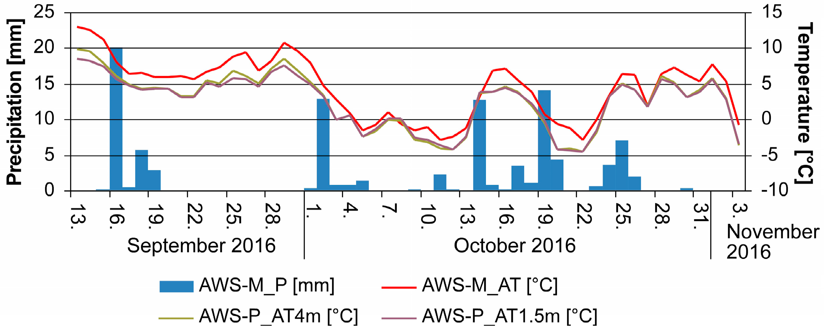
3.1.4. Meteorological Conditions and Ablation between the Two Field Campaigns

Two automatic weather stations (AWS) are located in close vicinity of the study area. One AWS (AWS-M) is located 1.9 km SE of the study area near the dammed lake Margaritze at 2070 m a.s.l. (see Figure 1). Air temperature (daily mean) and precipitation (daily sum) data from this station were provided for the period from 13 September 2016 to 3 November 2016 by Verbund AG. A second AWS (AWS-P) is located directly at the glacier surface 0.3 km W of the study area at about 2200 m a.s.l. (Figure 1). The Central Institute for Meteorology and Geodynamics, Vienna, provided air temperature data (recorded at 4 m and 1.5 m above the glacier surface) for the same period measuring at the site AWS-P.

Air temperature data can be used to estimate ice ablation in a given period by applying the degree-day model approach. This approach is based on the positive correlation between ablation and air temperature expressed as positive temperature sums or sum of thawing degrees [27]. The most common formulation (Equation (1)) combines the amount of ice melt (M in mm) during a period of n time intervals (∆t in d) with the sum of positive air temperatures of each time step (T+ in °C) during the same period and the factor of proportionality being the so-called degree-day factor (DDF in mm d⁻¹·°C⁻¹).

$${\displaystyle \sum }_{i=1}^{n}M=DDF{\displaystyle \sum }_{i=1}^{n}T+\mathsf{\Delta }t$$

(1)

In most cases a daily time interval is used. Reference [27] summarizes earlier published degree-day factors from glaciers and snow-covered basins.

3.2. Data Processing

The large amount of aerial photographs (see Section 3.1.1) was managed by using structure-from-motion (SfM) photogrammetry, which is a main asset of this increasingly popular approach [28]. The basic principle of the SfM approach is that the photographs record the object from different perspectives that are then automatically assembled to point clouds using image matching procedures [28,29,30]. The SfM approach was implemented using the commercial software Agisoft PhotoScan Professional (v. 1.2.5 2735). Due to requirements of the software, compressed photographs (JPEG) had to be used. The general steps and specific settings of processing were as follows: after creating a sparse dense cloud, a dense point cloud was generated using medium quality mode and so-called aggressive depth filtering. The latter means that minor surface details are filtered out [31]. According to [8], the reduced quality mode during dense point cloud generation does not considerably affect the DEM accuracy but leads to a reduced processing time. References [8,31] showed that aggressive filtering reduces minor surface details. In our case we do not focus on single surface spots and thus a smoothed DEM is acceptable. Accordingly, DEMs and orthophotos were generated with a ground sampling distance (GSD) of 0.04 m, but resampled to 0.15 m to keep the data size manageable.

DEM differencing was implemented (in ArcGIS v. 10.4) by subtracting the newer UAS DEM November 2016 minus the previous UAS DEM September 2016, each with a ground sampling distance of 0.15 m.

Based on orthophotos of both September 2016 and November 2016 (see Section 4.2), horizontal displacements were calculated using the normalized cross correlation (NCC) implemented by means of the software CIAS [32], see [33]. The displacement direction was smoothed using Inverse Distance Weighting (IDW). Some initial outliers were neglected in the further processing by visual identification and manual removal.

3.3. Accuracy Assessment

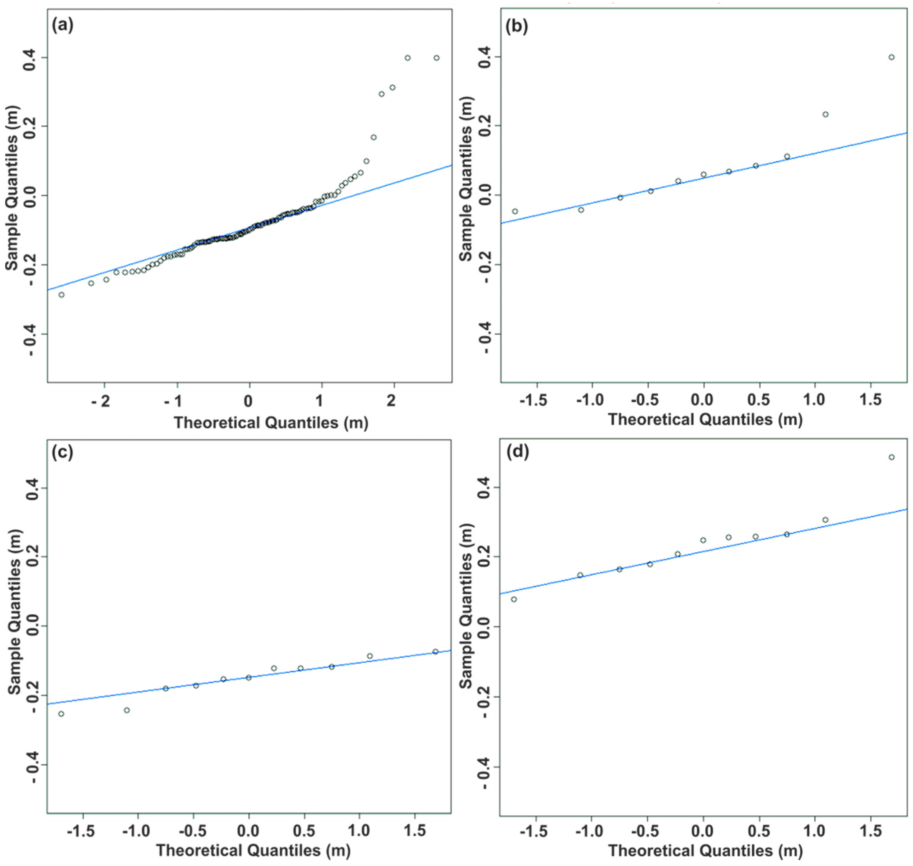
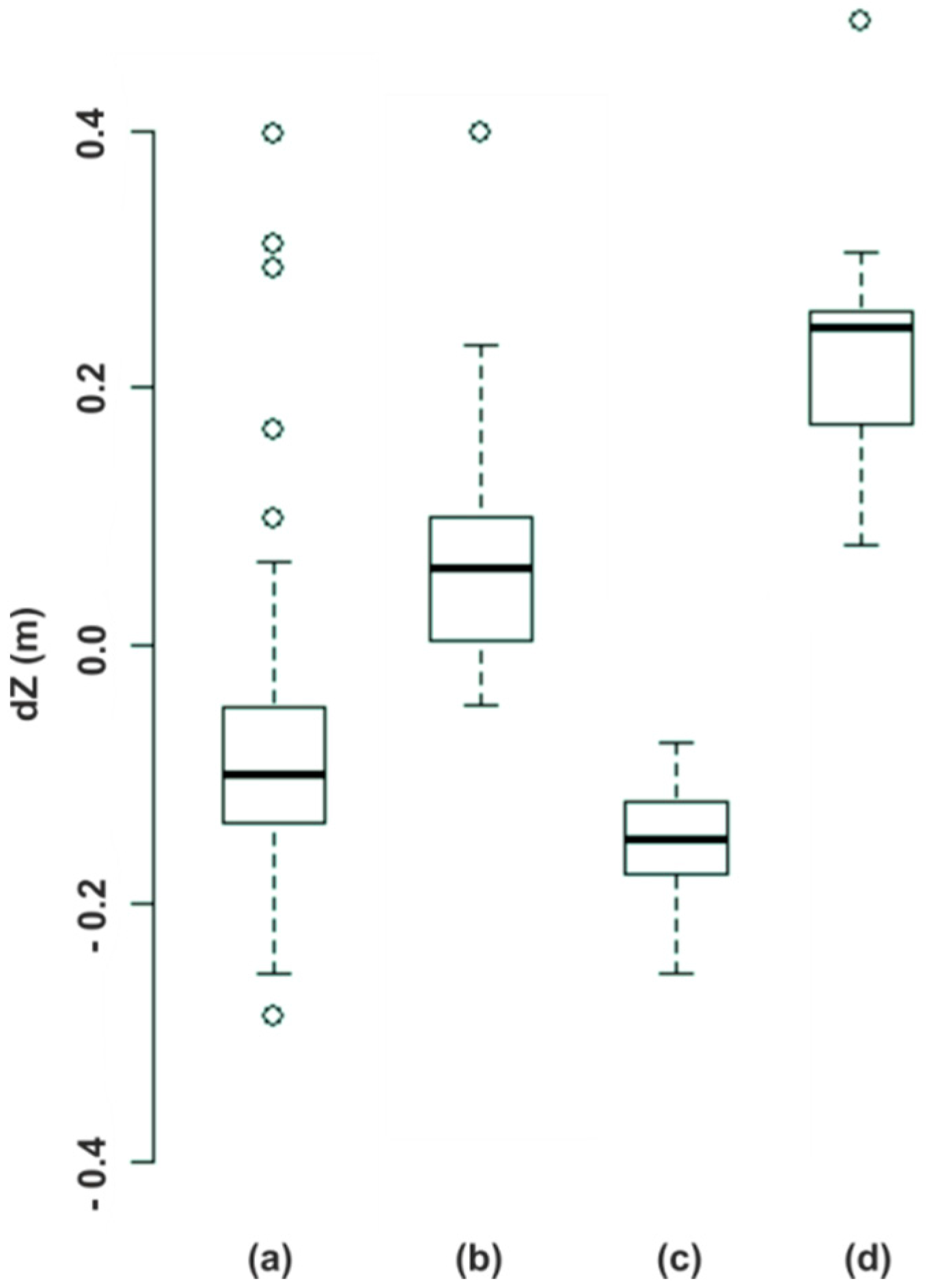
3.3.1. Independent Check Points

By using independent, i.e., not used during georeferencing, so-called check points (n = 104), an assessment of the accuracy of the photogrammetrically gained elevations of DEMs compared to geodetically measured DGPS points was made. In order to take into account the size and topography of the studied area, these points were well distributed around the study area (see Figure 4). The number of check points is small compared to the points calculated photogrammetrically. Yet, it is possible to make statements about the quality of our outcomes. This comparison was realized in the software package R (v. 3.3.1, www.r-project.org) and relates the quantiles of the empirical distribution to quantiles of the normal distribution in a quantile-quantile (Q-Q) plot, see [34]. Figure 6 gives an idea about the normal distribution of the sample data. Due to the fact that in most of these cases a normal distribution can be assumed, we can use the standard deviation (SD), which is in a range of ±0.06 m to 0.13 m, to describe the vertical accuracy of our DEMs. Figure 7 is based on the same sample data and, compared to the latter, more obviously indicates the range of elevation differences. These differences are related to the whole set of check point elevation values compared to elevations located at the same positions in the DEM of November 2016 (Figure 7a) and are in a range of approximately 0.05 m to 0.14 m concerning the interquartile range. A subsample of check points (geodetic profile A-B) was plotted in Figure 6b–d and Figure 7b–d and is also visualized in profile A-B in Section 3.3.3.

3.3.2. Root Mean Square Errors

The horizontal and vertical root mean square errors (RMSEs), resulting for the GCPs during photogrammetric processing, are visualized for both dates in Figure 8. The horizontal RMSEs (XY) are visualized as vectors and are in a range of a few centimeters. The vertical RMSEs (Z) are also in an order of magnitude of a few centimeters and were interpolated based on a spline using ArcGIS (v. 10.4). In general, no overall trend is recognizable even if the November-related vertical errors seem to be slightly higher at the boundaries of the area (see Figure 8b). We can point out that the result of the georeferencing is sufficiently accurate for the generated DEMs and orthophotos by taking the magnitude of the glacier surface changes (Section 4) into account. Corresponding to, e.g., [8] or [35], the relation of GCPs used per area unit is mainly influencing the DEM errors. We used 0.6 GCPs·ha⁻¹ (September 2016) and 0.4 GCPs·ha⁻¹ (September 2016), leading to the visualized RMSEs and therefore can expect accurate results.

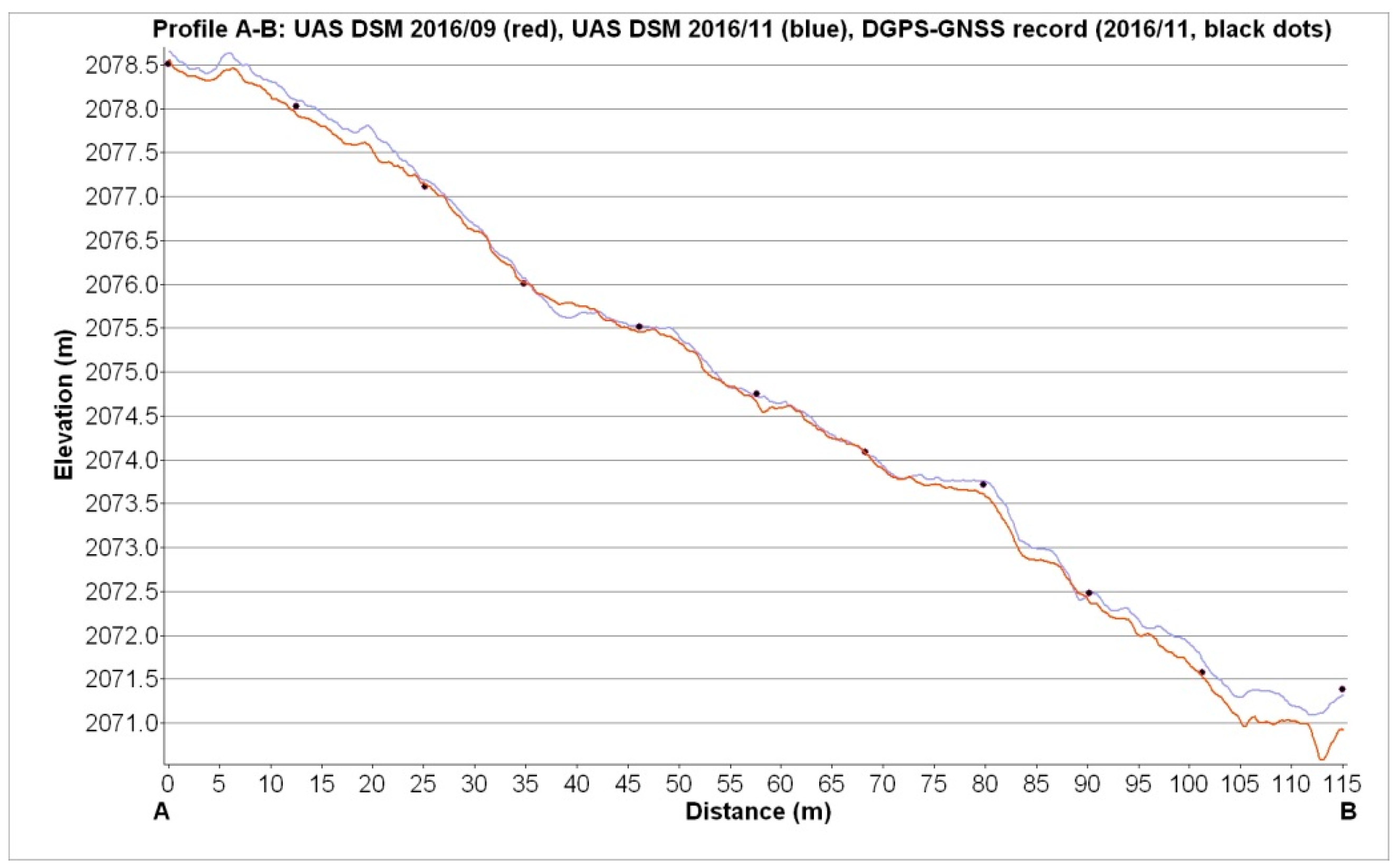
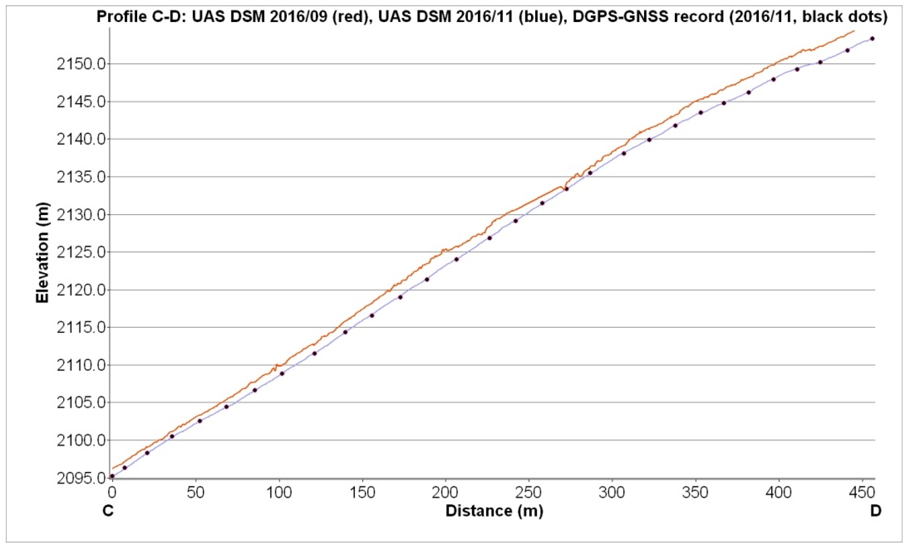
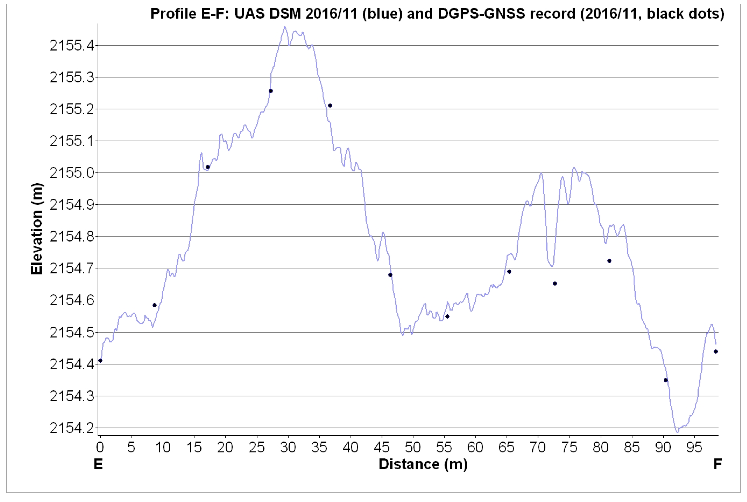
3.3.3. Geodetic Elevation Profile

Some of the geodetic check points, which are located in the debris-dominated proglacial area as well as on the partially debris-covered glacier tongue (see Figure 5) were subsampled to be shown in elevation profiles by comparison with the elevations of the DEMs. Figure 9 shows one of these subsamples and the differences (discussed in Section 3.3.1) in a profile located in the proglacial area. As indicated there, the geodetic point measurements correspond very well to the UAS DEM of November 2016 because the data was recorded on the same day. However, it is obvious that also the UAS DEM September 2016 matches most of the check points. A profile situated on the debris-covered central part of the glacier tongue is shown in Figure 10. This part of the glacier was not covered by photos during the flight campaign of September 2016 and hence only the comparison of the UAS DEM November 2016 and the respective check points is possible. This figure and the latter illustrate that the accuracy of the results is on an appropriately high level.

3.3.4. Displacement Vectors

The NCC-derived displacement vectors (see Section 3.2) were investigated at stable points (n = 1446), where no change was expected, e.g., bedrock areas, see [13]. However, there was a displacement of 0.17 m (mean) detected. That means that this measure describes the accuracy of the resulting orthophotos. On the other hand, the resulting displacement distances at the changing glacier surface were systematically overestimated. Consequently, this systematic offset was used to correct the displacement distances discussed in Section 4.3.

4. Results

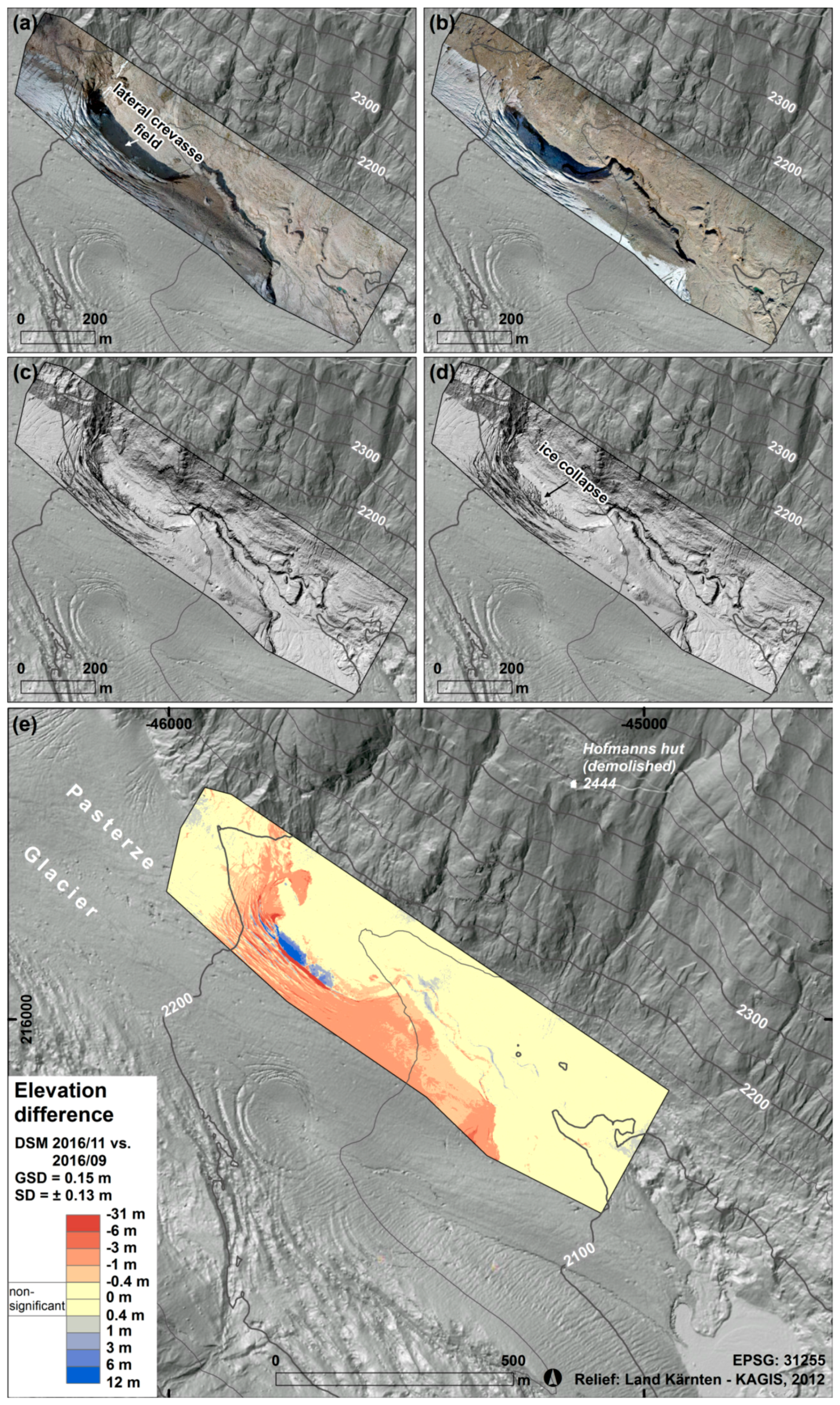
4.1. Elevation Difference Based on the Geodetic Profile

According to Section 3.3.3, a comparison of UAS DEM elevation values and corresponding geodetic elevation measurements can be used to assess the accuracy level reached. In this section the same approach of data comparison is performed but with a different motivation. Section 3.3.3 aims to show no differences in order to establish proof of the accuracy. This section attempts to highlight differences that indicate significant changes. Based on the differences shown in Figure 11, a glacier surface decrease of about −1 m during 51 days can be estimated along that profile line.

4.2. Elevation Difference Based on DEM Differencing

Figure 12a,b shows subsets of the orthophotos from September 2016 and November 2016. The lateral crevasse field can clearly be seen and by comparison, also the ice masses that collapsed in that period of time. Hillshades of UAS DEMs indicate the same ice collapse events (Figure 12c,d). The elevation difference is visualized in Figure 12e. The level of significant differences was assumed to the threefold SD and thus all differences below 0.4 m can be considered as non-significant. These areas dominate in the proglacial area, just as expected. On the other hand, the glacier surface is characterized by significant elevation decrease. In particular, the mentioned ice collapse is obvious with an elevation decrease of about 30 m. The collapsed ice masses led to accumulation and an elevation increase next to the crevasse field. A maximum value of increase of 12 m is the result of a partially sideways moving glacier (Figure 13). Apart from these apparent changes, some changes in the melt water channel are recognizable. But the channel is deeply incised and thus not ideal for photogrammetric processing. Therefore, it is questionable whether these are in fact significant changes. Furthermore, for the most northwestern part of that glacier subset, a significant elevation decrease cannot be shown.

Concerning the movement, the linear-like pattern of alternating increase and the decrease areas at the crevasse field also give a hint about the sideways movement. A mean glacier surface height decrease of −0.86 m (i.e., −0.017 m·d⁻¹) was detected by adding up the difference values of each grid cell. By using another approach (the surface volume tool in ArcGIS), a volume decrease of 113,963 m³ for that subset of the glacier tongue was calculated. This gives a mean surface height decrease of −0.95 m (i.e., −0.019 m·d⁻¹) in relation to the corresponding glacier area of about 0.12 km².

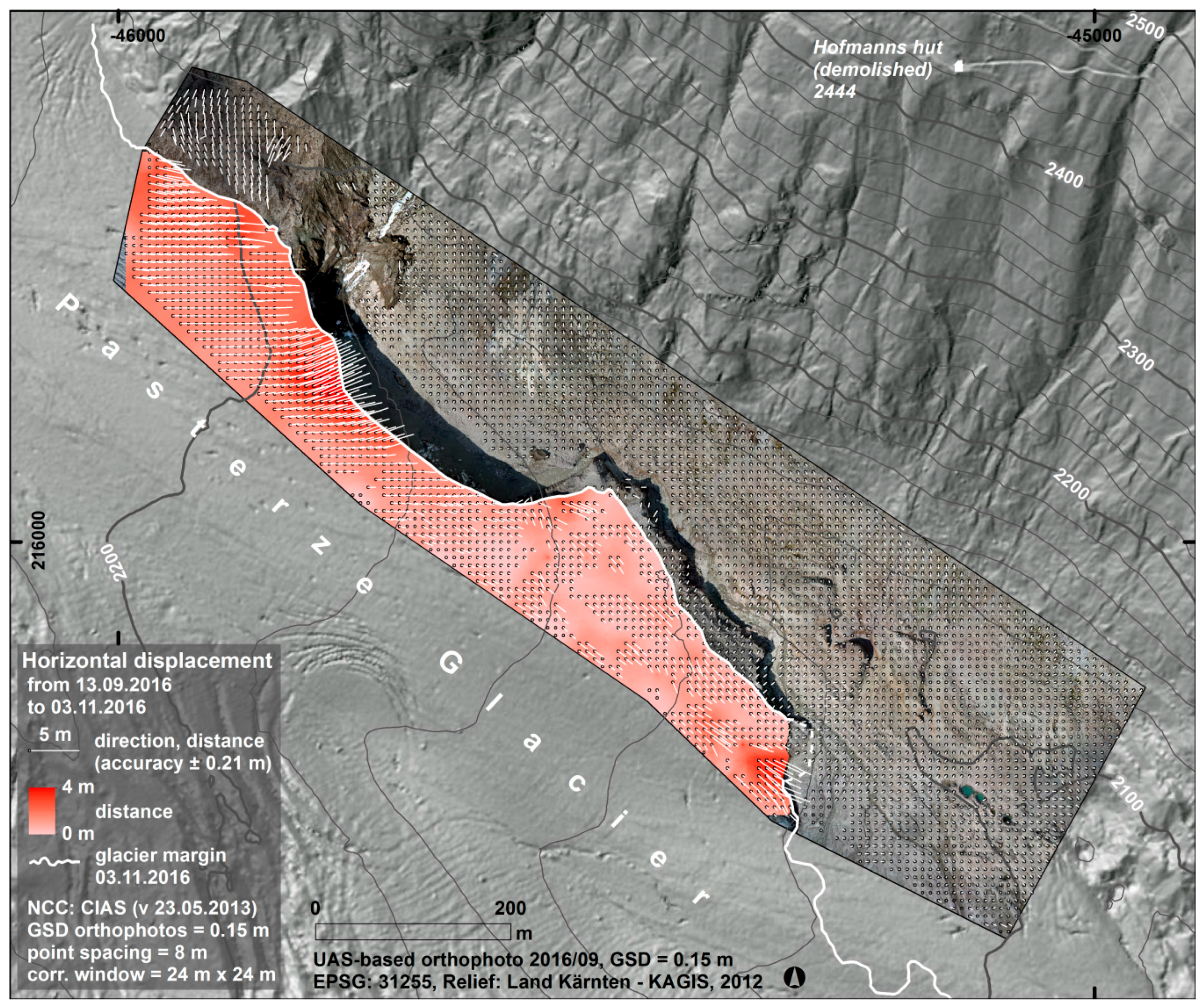
4.3. Horizontal Surface Displacement

The NCC-related and corrected results (see Section 3.2 and Section 3.3.4) indicate vectors of horizontal displacement (Figure 13). The mean distance of displacement of the glacier surface was 0.93 m, max. 3.5 m (n = 1092), for the period between 13 September 2016 and 3 November 2016. Concerning the direction of glacier movement, it is mentionable that apart from the general downward direction a WSW-ENE striking movement at the lateral crevasse field is noticeable, leading to further crevasse opening and to ice collapses. The distances of displacement (reddish color-scaled) show considerable movement at the lateral crevasse field, the very end of the glacier tongue, and the northwestern part of the processed glacier surface. The latter fact allows, by comparison with the elevation-based results, the statement that the most northwestern part of the glacier subset is characterized by remarkable movement and nearly unchanged glacier surface heights. The accuracy of displacement distances was assessed at stable points, see Section 3.3.4. Other than described there, here we used the SD (threefold SD of ±0.21 m).

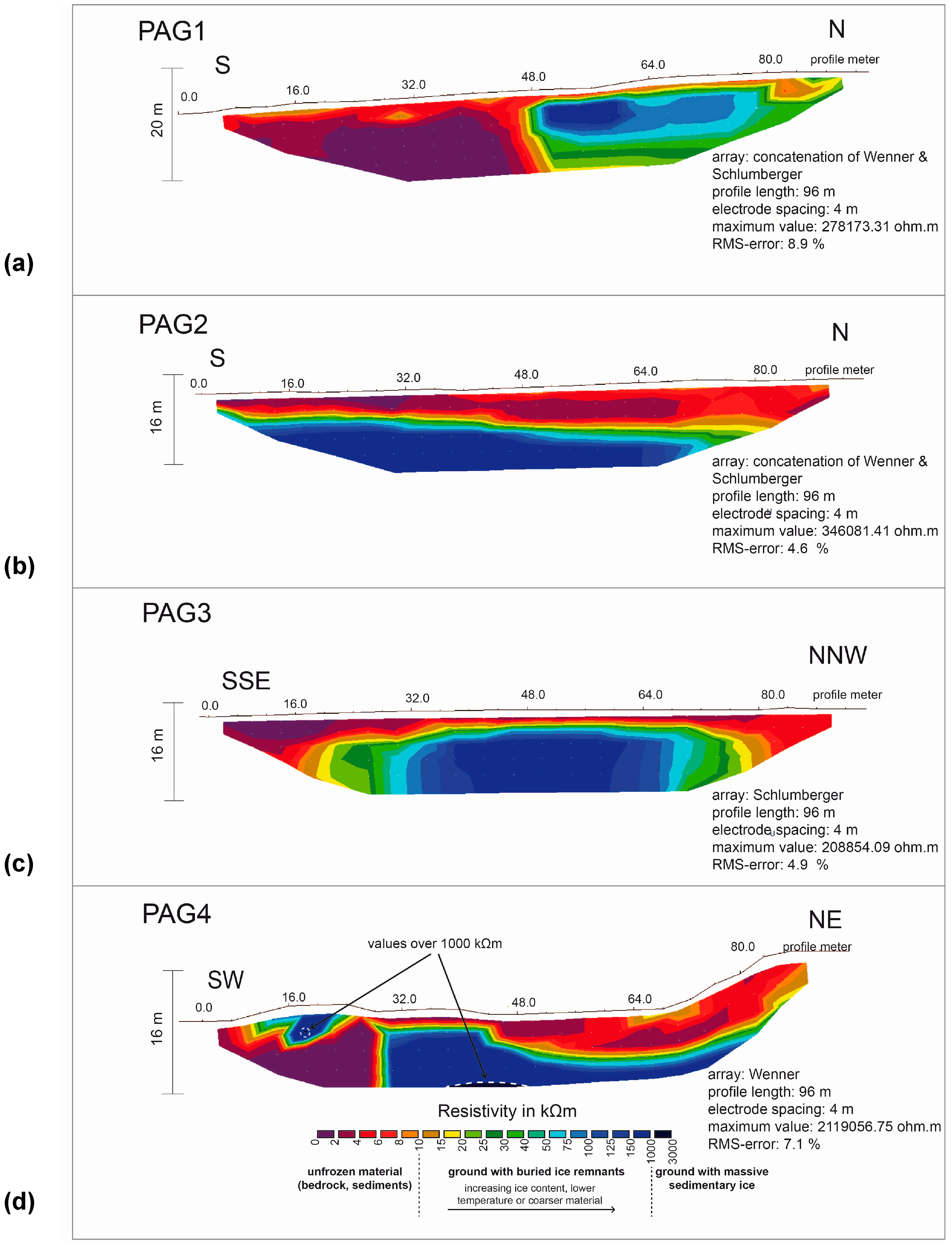
4.4. Electrical Resistivity Tomography Profiling

Figure 14 depicts the results at the four ERT profiles measured at the proglacial area of the Pasterze Glacier. For PAG1 and PAG2, the Wenner and Schlumberger measurements were concatenated yielding low RMS errors. For PAG3 only, the Schlumberger data were used. In contrast, for PAG4 only the Wenner data were used related to data quality and RMS errors. The lowest resistivity values at all four profiles are in the order of 260 to 870 resistivity ohm.m related to the unfrozen sediments. The highest resistivity values vary between 208,000 ohm.m at PAG3 to 2,119,000 ohm.m at PAG4 (

Table 1. Measured values of electric resistivity of profiles 1 to 4 (see Figure 5 and Figure 15).

Profile	Date	Used Arrays for Analyses 1	Max. (ohm.m)	Min. (ohm.m)
PAG1	13 September 2016	Wen, Schlu	278,173	800
PAG2	13 September 2016	Wen, Schlu	346,081	870
PAG3	13 September 2016	Schlu	208,854	776
PAG4	13 September 2016	Wen	2,119,057	258

¹ Wen = Wenner, Schlu-Schlumberger.

). The highest values at the remaining two profiles are 278,000 ohm.m (PAG1) and 346,000 ohm.m (PAG2).

4.5. Meteorological Conditions and their Effect on Glacier Ice Ablation

Figure 15 depicts the atmospheric conditions during the 51 days between the two UAS campaigns. The mean air temperature for this period was 4.5 °C at AWS-M, 2.7 °C at AWS-P at 4 m from the surface, and finally 2.6 °C at AWS-P at 1.5 m from the surface. The highest mean daily temperatures were in the range of 8.6 °C (AWS-P_1.5m) to 13.0 °C (AWS-M). The difference of the two values suggests substantially higher temperatures in the proglacial area compared to the glacier surface. However, the large difference of 4.4 °C was partly also related to the difference in elevation of the two AWS sites (ca. 130 m). Furthermore, the air temperature (AT) at AWS-P at 1.5 m above the glacier surface was on average slightly cooler compared to the sensor at 4 m above the glacier surface. The mean air temperature was only negative during 12 (AWS-M) to 15 days (AWS-P_AT4m) during the 52-day period. No precipitation was measured during 27 days of the 52-day period. The described meteorological conditions indicate glacier ablation-favorable conditions for the period between the two flights.

The meteorological conditions measured at the 1.5 m sensor at AWS-P are most likely valid for the glacier-covered part of the two flight campaigns related to its proximity and the same surface characteristics. Using Equation (1), the number of days (52), and the positive air temperatures of each time step measured during that period at AWS-P_1.5m, one receives DDF-values at debris-free, little moving, and crevasse-poor glacier surfaces in the range of 10.6 mm·d⁻¹·°C⁻¹ for −1.8 m of ice ablation to 7.9 mm·d⁻¹·°C⁻¹ for −1.35 m of ice ablation.

5. Discussion

Apart from usual terrestrial methods, DEMs are an important database for glaciological studies. High spatial resolution, as achieved by using UAS, is one component when using remote sensing techniques. Even though in that case the high resolution data was only gained for a comparably small subset of the entire glacier extent, it was possible to indicate the applicability of UAS for glacier studies, even in a high alpine environment.

The DEMs’ accuracy level reached is in the same range as in other UAS studies, both related to glaciers [8] or other topics [19,35]. One main reason for that is the density of GCP measurements that in our case was about 0.5 GCPs·ha⁻¹ and matches well the results in a similar order of magnitude, e.g., [8,19,35]. Reference [36] highlights the need for visualization of DEM error estimates, e.g., RMSE, in order to check for potentially systematic errors. In Section 3.3.2, we showed GCP-related RMSEs in a spatial context and therefore agree with this approach, which was already used by, e.g., [19]. However, amongst the methods used for assessing the DEMs’ accuracy in this study, the usage of independent check points is probably the most valuable method. However, using a variety of assessing methods, such as that described in Section 3.3, is recommended to make error estimates more convincing. The results of the glacier surface changes are able to confirm the glacier changes outlined, e.g., in [9] or [13].

By using air temperature data from a nearby AWS located at the glacier surface and our results from the two DEMs, we calculated DDF-values at debris-free and crevasse-poor glacier surfaces in the range of 10.6 to 7.9 mm·d⁻¹·°C⁻¹. A similar DDF value of 11.7 mm·d⁻¹·°C⁻¹ for ice was calculated for the Aletsch Glacier in Switzerland [37]. More generally, [38] reported that the DDF is commonly on the order of between 4 and 8 mm·d⁻¹·°C⁻¹ at alpine glaciers [37,38]. Therefore our results fit rather well into the earlier DDF-value calculations.

We calculated the DDF for continuously debris-covered and crevasse-poor glacier surfaces using the same equation and station data. At glacier surfaces with a surface elevation change of −0.5 m between the two campaigns, a DDF of 2.9 mm·d⁻¹·°C⁻¹ was revealed. This value increases to 5.9 mm·d⁻¹·°C⁻¹ if a location with a surface elevation change of −1.0 m is considered. However, the big uncertainty in this consideration is the unknown supraglacial debris cover thickness at the considered sites. As known from earlier studies [16], the thickness of the supraglacial debris cover at the Pastere Glacier is generally far below 1 m, but thickening continuously from near the ice fall to the glacier terminus. Furthermore, debris cover thickness might vary substantially over short distances related to former crevasses which were later filled by supraglacial sediments [16].

The existence of permafrost in the proglacial area of the Pasterze Glacier covered by the two UAS-campaigns is very unlikely. This was shown, e.g., by an earlier study which indicated the existence of permafrost at much higher elevations in the Pasterze Glacier-area [39]. Therefore, the tongue of Pasterze Glacier consists of temperate ice and permafrost is absent. Massive sedimentary (or “glacier”) ice is characterized by resistivity values in the range of 10⁶ to 10⁸ ohm.m [20]. Values < 10⁶ ohm.m might indicate rather little lenses of dead ice in the proglacial area of the Pasterze Glacier. Furthermore, a high debris content of a buried massive ice body (e.g., infills of former glacier crevasses, or former thrust faults with debris) might substantially lower the resistivity values as well.

Therefore, as judged from these considerations and our results depicted in Figure 14, we assume rather little glacier-ice remains in profile PAG1, possibly still connected with the main glacier tongue. In profiles PAG2 and PAG3, larger masses of buried, debris-mixed glacier ice seems to exist below an ice-free debris cover with a thickness of a few meters. Profile PAG4 is clearly different compared to the other three profiles, with maximum values far above 10⁶ ohm.m (max. 2,119,000 ohm.m). The largest buried dead-ice masses were found at this profile. However, the debris cover burying the glacier ice remnant is several meters thick in most places along the profile as judged from the ERT data, thus protecting the underlying ice from the warm atmospheric conditions at the surface. In general, the surface elevation in the proglacial area around the four ERT profiles changed only to a very small extent with the maximum surface elevation lowering values on the order of 20 cm at profile PAG2 and rather stable conditions at the other three profiles. This suggests efficient buried-ice protection by the debris layer during the observation period.

6. Conclusions

We used a UAS to detect surface changes of a subset of the Pasterze Glacier and parts of its proglacial area. By using different methodological approaches for assessing the DEMs’ accuracy, we found that the resulting DEMs and orthophotos are sufficiently accurate with respect to the detected changes. Thus, the following can be concluded:

• Based on DEM differencing, we calculated a mean glacier surface height lowering of −0.9 m, i.e., −0.02 m·d⁻¹.
• We detected a mean glacier surface movement of 0.93 m, max. 3.5 m, i.e., 0.02 m·d⁻¹, max. 0.07 m·d⁻¹.
• The glacier movement forced ice collapses at a lateral crevasse field leading to a maximum elevation decrease of −31 m. The most northwestern section of the studied glacier parts are characterized by surface movement only, whereas a substantial surface height lowering did not occur.
• By calculating the DDF-values and comparing these values with earlier studies, we were able to quantify the ablation rates as typical for a high alpine glacier in the European Alps.
• We delineated the glacier margin manually by using our orthophotos. However, for some parts of the glacier terminus, we were able to correct our mapping based on ERT measurements which revealed debris-covered glacier ice possibly still connected to the glacier tongue. Therefore, this geophysical approach is valuable to be applied in addition to UAS flight campaigns.
• The surface of the proglacial area did not substantially change, with one exception in the most northwestern part of the studied area. The glacial and proglacial transition zone behaves like the proglacial area with a nearly non-changing surface as indicated by UAS-based DEMs. As shown by ERT measurements, the underlying material—glacier ice or dead ice—does not influence the debris-covered surface behavior.

We therefore argue that UAS are an appropriate tool for glacier studies even though the usage is limited. Consequently, by doing further flight campaigns we will expand the methodological spectrum of regular glacier measurements at the Pasterze Glacier.

References

- Bernard, É.; Friedt, J.M.; Tolle, F.; Marlin, C.; Griselin, M. Using a small COTS UAV to quantify moraine dynamics induced by climate shift in Arctic environments. Int. J. Remote Sens. 2017, 38, 2480–2494. [Google Scholar] [CrossRef]
- Colomina, I.; Molina, P. Unmanned aerial systems for photogrammetry and remote sensing: A review. ISPRS J. Photogramm. Remote Sens. 2014, 92, 79–97. [Google Scholar] [CrossRef]
- Pajares, G. Overview and current status of remote sensing applications based on unmanned aerial vehicles (UAVs). Photogramm. Eng. Remote Sens. 2015, 81, 281–329. [Google Scholar] [CrossRef]
- Bhardwaj, A.; Sam, L.; Martín-Torres, F.J.; Kumar, R. UAVs as remote sensing platform in glaciology: Present applications and future prospects. Remote Sens. Environ. 2016, 175, 196–204. [Google Scholar] [CrossRef]
- Immerzeel, W.W.; Kraaijenbrink, P.D.A.; Shea, J.M.; Shrestha, A.B.; Pellicciotti, F.; Bierkens, M.F.P.; de Jong, S.M. High-resolution monitoring of Himalayan glacier dynamics using unmanned aerial vehicles. Remote Sens. Environ. 2014, 150, 93–103. [Google Scholar] [CrossRef]
- Friedli, E. Photogrammetric Methods for the Reconstruction and Monitoring of Glaciers. Master’s Thesis, ETH Zürich, Zürich, Switzerland, 28 January 2013. [Google Scholar]
- Santagata, T. Using Unmanned Aerial Vehicles for monitoring glacial moulins. Geophys. Res. Abstr. 2016, 18, EGU2016-3875-1. [Google Scholar]
- Gindraux, S.; Boesch, R.; Farinotti, D. Accuracy Assessment of Digital Surface Models from Unmanned Aerial Vehicles’ Imagery on Glaciers. Remote Sens. 2017, 9, 186. [Google Scholar] [CrossRef]
- Wakonigg, H. Die Nachmessungen an der Pasterze von 1879 bis 1990. Arb. Geogr. Inst. Graz 1991, 30, 271–307. [Google Scholar]
- Lieb, G.K. Die Pasterze: 125 Jahre Gletschermessungen und ein neuer Führer zum Gletscherweg. Grazer Mitt. d. Geogr. u. R. 2004, 34, 3–5. [Google Scholar]
- Wakonigg, H.; Tintor, W. Zum Massenumsatz der Pasterzenzunge zwischen 1979 und 1994. Wiss. Mitt. a. d. Nationalpark Hohe Tauern 1999, 5, 193–203. [Google Scholar]
- Kaufmann, V.; Kellerer-Pirklbauer, A.; Kenyi, L.W. Gletscherbewegungsmessung mittels satellitengestützter Radar-Interferometrie: Die Pasterze (Glocknergruppe, Hohe Tauern, Kärnten). Zeitschr. f. Gletscherkunde u. Glazialgeologie 2008, 42, 85–104. [Google Scholar]
- Kaufmann, V.; Kellerer-Pirklbauer, A.; Lieb, G.K.; Slupetzky, H.; Avian, M. Glaciological Studies at Pasterze Glacier (Austria) Based on Aerial Photographs. In Monitoring and Modeling of Global Changes: A Geomatics Perpectic; Li, J., Yang, X., Eds.; Springer: Dordrecht, The Netherlands, 2015; pp. 173–198. [Google Scholar]
- Gspurning, J.; Tintor, W.; Tribuser, M.; Wakonigg, H. Volumen- und Flächenänderungen an der Pasterze von 1981 bis 2000. Carinthia II 2004, 194, 463–472. [Google Scholar]
- Kellerer-Pirklbauer, A.; Lieb, G.K.; Avian, M.; Gspurning, J. The response of partially debris-covered valley glaciers to climate change: the example of the Pasterze Glacier (Austria) in the period 1964 to 2006. Geogr. Ann. 2008, 90, 269–285. [Google Scholar] [CrossRef]
- Kellerer-Pirklbauer, A. The Supraglacial Debris System at the Pasterze Glacier, Austria: Spatial Distribution, Characteristics and Transport of Debris. Ann. Geomorph. 2008, 52 (Suppl. S1), 3–25. [Google Scholar] [CrossRef]
- Remondino, F.; Barazzetti, L.; Nex, F.; Scaioni, M.; Sarazzi, D. UAV Photogrammetry for Mapping and 3D Modeling—Current Status and Future Perspectives. Int. Arch. Photogramm. Remote Sens. Spat. Inf. Sci. 2011, XXXVIII-1/C22, 25–31. [Google Scholar] [CrossRef]
- Schöttl, S.; Seier, G.; Rascher, E.; Sulzer, W.; Sass, O. UAS-Based Quantification of Sedimentary Body Changes at Langgriesgraben, Styria, Austria. Geoph. Res. Abstr. 2016, 18, EGU2016-15077-1. [Google Scholar]
- Seier, G.; Stangl, J.; Schöttl, S.; Sulzer, W.; Sass, O. UAV and TLS for monitoring a creek in an alpine environment, Styria, Austria. Int. J. Remote Sens. 2017, 38, 2903–2920. [Google Scholar] [CrossRef]
- Kneisel, C.; Hauck, C. Electrical methods. In Applied Geophysics in Periglacial Environments; Hauck, C., Kneisel, C., Eds.; Cambridge University Press: Cambridge, UK, 2008; pp. 3–27. [Google Scholar]
- Kneisel, C. New Insights into Mountain Permafrost Occurrence and Characteristics in Glacier Forefields at High Altitude through the Application of 2D Resistivity Imaging. Permafr. Periglac. Process. 2004, 15, 221–227. [Google Scholar] [CrossRef]
- Bosson, J.-B.; Deline, P.; Bodin, X.; Schoeneich, P.; Baron, L.; Gardent, M.; Lambiel, C. The influence of ground ice distribution on geomorphic dynamics since the Little Ice Age in proglacial areas of two cirque glacier systems. Earth Surf. Process. Landf. 2015, 40, 666–680. [Google Scholar] [CrossRef]
- Lieb, G.K.; Kellerer-Pirklbauer, A. Die Pasterze, Österreichs größter Gletscher, und seine lange Messreihe in einer Ära massiven Gletscherschwundes. In Geschichte Des Ewigen Eises; Fischer, A., Ed.; Springer: Berlin/Heidelberg, Germany, 2017; in press. [Google Scholar]
- Wakonigg, H.; Lieb, G.K. Die Pasterze und ihre Erforschung im Rahmen der Gletschermessungen. Kärntner Nationalpark Schr. 1996, 8, 99–115. [Google Scholar]
- Verhoeven, G.J.J. It’s all about the format—Unleashing the power of RAW aerial photography. Int. J. Remote Sens. 2010, 31, 2009–2042. [Google Scholar] [CrossRef]
- Loke, M.H. Electrical Imaging Surveys for Environmental and Engineering Studies—A Practical Guide to 2-D and 3-D Surveys; RES2DINV Manual: Penang, Malaysia, 2000; p. 67. [Google Scholar]
- Hock, R. Temperature index melt modelling in mountain areas. J. Hydrol. 2003, 282, 104–115. [Google Scholar] [CrossRef]
- Fonstad, M.A.; Dietrich, J.T.; Courville, B.C.; Jensen, J.L.; Carbonneau, P.E. Topographic Structure from Motion: A New Development in Photogrammetric Measurement. Earth Surf. Process. Landf. 2013, 38, 421–430. [Google Scholar] [CrossRef]
- Westoby, M.J.; Brasington, J.; Glasser, N.F.; Hambrey, M.J.; Reynolds, J.M. ‘Structure-From-Motion’ Photogrammetry: A Low-Cost, Effective Tool for Geoscience Applications. Geomorphology 2012, 179, 300–314. [Google Scholar] [CrossRef]
- Micheletti, N.; Chandler, J.H.; Lane, S.N. Structure from Motion (Sfm) Photogrammetry. In Geomorphological Techniques; Cook, S.J., Clarke, L.E., Nield, J.M., Eds.; British Society for Geomorphology: London, UK, 2015; pp. 1–12. ISBN 2047-0371. [Google Scholar]
- Peppa, M.V.; Mills, J.P.; Moore, P.; Miller, P.E.; Chambers, J.E. Accuracy Assessment of a UAV-Based Landslide Monitoring System. Int. Arch. Photogramm. Remote Sens. Spat. Inf. Sci. 2016, XLI-B5, 895–902. [Google Scholar] [CrossRef]
- Image Correlation Software CIAS. Available online: http://www.mn.uio.no/geo/english/research/projects/icemass/cias (accessed on 18 December 2016).
- Debella-Gilo, M.; Kääb, A. Sub-pixel precision image matching for measuring surface displacements on mass movements using normalized cross-correlation. Remote Sens. Environ. 2011, 115, 130–142. [Google Scholar] [CrossRef]
- Höhle, J.; Höhle, M. Accuracy Assessment of Digital Elevation Models by Means of Robust Statistical Methods. ISPRS J. Photogramm. Remote Sens. 2009, 64, 398–406. [Google Scholar] [CrossRef]
- Coveney, S.; Roberts, K. Lightweight UAV digital elevation models and orthoimagery for environmental applications: Data accuracy evaluation and potential for river flood risk modelling. Int. J. Remote Sens. 2017, 38, 3159–3180. [Google Scholar] [CrossRef]
- James, M.R.; Robson, S.; d’Oleire-Oltmanns, S.; Niethammer, U. Optimising UAV topographic surveys processed with structure-from-motion: Ground control quality, quantity and bundle adjustment. Geomorphology 2017, 280, 51–66. [Google Scholar] [CrossRef]
- Lang, H. Forecasting meltwater runoff from snow-covered areas and from glacier basins. In River Flow Modelling and Forecasting; Kraijenhoff, D.A., Moll, J.R., Eds.; D. Reidel Publishing Company: Dordrecht, The Netherlands, 1986; pp. 99–127. [Google Scholar]
- Kuhn, M. Die Reaktion der österreichischen Gletscher und ihres Abflusses auf Änderungen von Temperatur und Niederschlag. Österr. Wasser- u. Abfallwirtschaft 2004, 56, 1–17. [Google Scholar]
- Kellerer-Pirklbauer, A.; Lieb, G.K.; Avian, M.; Carrivick, J. Climate change and rock fall events in high mountain areas: Numerous and extensive rock falls in 2007 at Mittlerer Burgstall, Central Austria. Geografiska Annaler 2012, 94, 59–78. [Google Scholar] [CrossRef]