
Impervious Surface Information Extraction Based on Hyperspectral Remote Sensing Imagery


1
Island Research Center, State Oceanic Administration, Pingtan 350400, China
2
College of Environment and Resources, Fuzhou University, Fuzhou 350116, China
*
Author to whom correspondence should be addressed.
Remote Sens. 2017, 9(6), 550; https://doi.org/10.3390/rs9060550
Submission received: 29 March 2017
/
Revised: 23 May 2017
/
Accepted: 26 May 2017
/
Published: 1 June 2017
Abstract
:The retrieval of impervious surface information is a hot topic in remote sensing. However, researches on impervious surface retrieval from hyperspectral remote sensing imagery are rare. This paper illustrates a case study of information extraction from urban impervious surfaces based on hyperspectral remote sensing imagery that is intended to improve the image spectral resolution of impermeable materials. Fuzhou, Guangzhou, and Hangzhou were selected as test areas and EO-1 Hyperion images were used as data sources. The impervious surface features were retrieved from remote sensing images using linear spectral mixture analysis. A stepwise discriminant analysis was performed to select feature bands for impervious surface retrieval. A standard deviation analysis, correlation analysis, and principal component analysis were then carried out for each of those up to 158 valid Hyperion spectral bands. Eleven feature bands were selected using the stepwise discriminant analysis and a new image called Hyperion’ was formed. The impervious surface was then retrieved from Hyperion’. The results indicate that the extraction accuracy and coverage accuracy are high in all three test areas. Tests of eleven feature band combinations selected in different areas show very good representations of the band combinations in impervious surface retrieval, and can thus be used as optimal band combinations for impervious surface retrieval.

1. Introduction
Major changes have occurred on the Earth’s surface as a result of rapid worldwide urbanization. Impervious surfaces have gradually replaced the natural landscape, causing a series of serious ecological and environmental problems, including reduced surface transpiration and evapotranspiration, increased runoff, blocked heat exchange, and biodiversity destruction [1,2,3]. Therefore, the ability to determine accurate information about impervious surface distributions in a timely manner has major significance for environmental and natural resource protection and governmental-level scientific decision-making.
In recent years, multispectral, hyperspectral, high spatial resolution, and other multi-source remote sensing images have provided a powerful tool for multi-scale and rapid monitoring of impervious surfaces. At present, many researchers are engaged in extensive studies of impervious surface information extraction methods, including mainly: (1) spectral mixture analysis; (2) impervious surface indexes; (3) multiple regression; (4) the classification and regression tree (CART) algorithm; and (5) classification. The spectral mixture analysis decomposes a pixel into fractional basic components named endmembers, assuming that the pixel spectrum is a linear or nonlinear combination of the spectra of all endmembers within the pixel [4,5]. The impervious surface indexes are used to enhance and extract impervious surfaces through remote sensing spectral indexes, including NDISI [6], BCI [7], and P index [8], etc. The multiple regression approach is based on the significant negative correlation between the impervious surface and vegetation [9]. The CART produces a rule-based model for the prediction of continuous variables based on training data, and yields the spatial estimates of subpixel percentage imperviousness [10,11,12]. The classification is based on the conventional remote sensing classification methods such as the support vector machine (SVM) [13,14,15], object based image analysis (OBIA) [16,17], and artificial neural networks (ANNs) [18,19].
Linear spectral mixture analysis (LSMA) is currently the main technology used for the extraction of impervious surface information in cities. The technology is largely based on the vegetation-impervious surface-soil (V-I-S) model proposed by Ridd [20]. Each pixel in a city area is considered as a linear combination of the three endmembers, i.e., the impervious surface, vegetation, and soil contents. Wu used the LSMA model and minimum noise fraction (MNF) conversion to estimate the impervious surface information from Landsat-7 Enhanced Thematic Mapper plus (ETM+) images within Columbus, OH, in the United States. The total root-mean-square error of the method was 10%, but with the premise that the soil and water information must be masked in advance [5,21]. Powell proposed a type of spectral decomposition model with multiple endmembers, retrieved the impervious surface coverage from ETM+ images, and obtained good results [22]. Yang used the LSMA method with multiple endmembers to obtain impervious surface information from the area of Lake Kasumigaura in Japan. The total root-mean-square error was reduced by 5.2%, but some high and low impervious surface areas were still undervalued or overestimated [23]. Lu used the LSMA model to obtain the impervious surfaces in a rural-urban fringe district, and the results showed that the impervious surface values in the rural-urban fringe district were overestimated by 50–60% [24]. In China, Zhou also used the LSMA model to obtain the impervious surface area distribution in Fuzhou from ETM+ images [25]. Zhao decomposed the mixed pixels of a Thematic Mapper (TM) image of Xiamen and found that a four-end-member method that included water could obtain better results, but spectral confusion between the vegetation on shady slopes and impervious surfaces was still serious [26]. Li used the LSMA model to retrieve impervious surface information from an ETM+ image of Hangzhou, and the results showed that impervious surfaces with low albedo were mixed with water and shadow, while impervious surfaces with high albedo were mixed with sand and bare soil [27].
Overall, the LSMA-based studies described above cannot distinguish an impervious surface from soil, water, and vegetation shadow to varying extents. Careful analysis shows that most of the existing studies are based on TM/ETM+, Advanced Spaceborne Thermal Emission and Reflection Radiometer (ASTER), and other multispectral remote sensing data. Because this type of imaging spectrum has a low resolution, it is difficult to reflect the spectral features of impervious surfaces and other surface features accurately, which leads to misclassification. Obviously, this problem can be solved by simply increasing the spectral resolution, but there are few current studies that use hyperspectral remote sensing images for impervious surface selection. For this reason, this study will use hyperspectral remote sensing data from the Earth Observing-1 Mission (EO-1) satellite’s Hyperion imaging spectrometer as a data source to determine feature bands that can be used to distinguish impervious surfaces from other surface features in the 242 Hyperion bands and thus improve the retrieval accuracy for impervious surfaces. The impervious surface features were derived using the LSMA model. This has important scientific significance for the improvement of the current impervious surface extraction model.
2. Data Sources and Preprocessing
2.1. Data Source
A Hyperion image of Fuzhou taken in 2003 was selected as the test area. To avoid the production of accidental test results, Hyperion images of both Guangzhou and Hangzhou were selected for verification. IKONOS and Google Earth images were used for accuracy validation. The original images of the three areas are shown in Figure 1. The data source and the purpose of the tests are shown in Table 1.
2.2. Study Area
Fuzhou City is located in southeastern China, and is the capital city of the Fujian province. It is also the center city of the Western Taiwan Straits Economic Zone. The approximate geographic position of the central city is 119°17′46′′E and 26°04′35′′N. For the past ten years, the city scale has expanded unceasingly. The total area of the city is 11,968 km2, and the urbanization rate was 66.8% in 2014.
Hangzhou City is the capital city of the Zhejiang province, located in eastern China. The approximate geographic position of the central city is 120°12′20′′E and 30°16′33′′N. It is one of the center cities in the urban agglomeration of the Yangtze River delta. The famous scenic area in Hangzhou is the West Lake.
Guangzhou City is the capital city of the Guangdong province, located in southern China. The approximate geographic position of the central city is 113°15′51′′E and 23°07′47′′N. The State Council positioned Guangzhou as one of the national central cities in 2010. Guangzhou was also appraised as the fastest-growing large city in the world by the United Nations.
Overall, these cities have very important positions in China, and are all the centers in their respective regional area. The urbanization phenomenon characterized by the expansion of the impervious surface is very typical, so we chose these three cities as the study areas.
2.3. Data Processing
First, the Hyperion image bands were selected, and 242 bands were checked individually. The bands without radiation calibration, which were severely affected by water vapor and carbon dioxide, with visible and near-infrared (VNIR) and short-wavelength infrared (SWIR) overlap, with a high frequency of band noise, and with poor data quality were removed. In the three test areas, 158 valid bands were ultimately retained, including Bands 8–57 (426–925 nm), Bands 79–119 (932–1336 nm), Bands 133–164 (1477–1790 nm), Bands 183–184 (1981–1991 nm), and Bands 188–220 (2032–2355 nm). The Fast Line-of-Sight Atmospheric Analysis of Spectral Hypercubes (FLAASH) model was used for the atmospheric correction of the Hyperion images. When combined with the Moderate Resolution Transmittance-type MODTRAN4+ radiation transfer model code, it can quickly correct the process effects caused by diffuse reflection, and thus eliminates the effects of water vapor, carbon dioxide, aerosols, and other particles in the atmosphere on the surface reflectance properties of features. This model can further convert radiation images into reflectance images.
3. Methods and Results
3.1. Selection of Hyperion Feature Bands
The narrow bands in hyperspectral images cause a high correlation and data redundancy between adjacent bands. Therefore, the 158 valid bands must be screened, and the most suitable feature band combinations for impervious surface retrieval should then be selected. It is necessary to comply with three principles in the selection process. First, the selected bands should contain large amounts of information. Second, the correlations among these feature bands should be as low as possible. Third, the spectral differences of the different features should be obvious. Based on the above principles, stepwise discriminant analysis was used to select the most appropriate feature bands, and the standard deviations, correlations of the 158 bands of the Hyperion image, and principal component analysis were also analyzed.
3.1.1. Stepwise Discriminant Analysis (SDA)
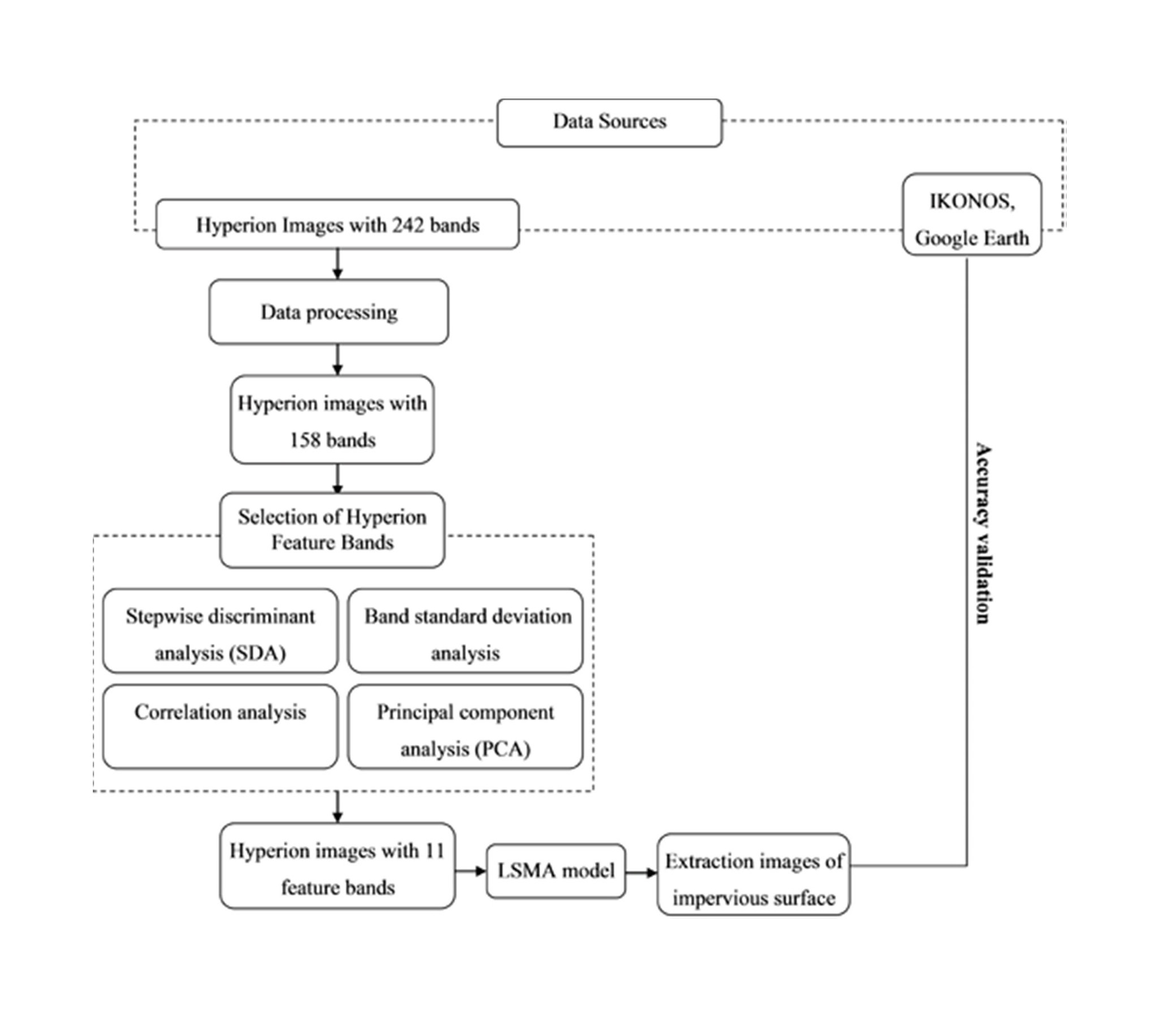
The Hyperion feature bands are mainly selected using the SDA method. Stepwise selection was imitated with no variable in the model. At each step, if a band in the model failed to meet the criterion (f test), the worst variable was removed. Otherwise, the band that contributed most to the discriminatory power of the model was entered. When all variables in the model met the criteria and the remaining variables were excluded, the stepwise selection process was stopped [28]. In SDA, the standard for introducing or eliminating variables is measured using Wilk’s Lambda, which is denoted by Λ. This is a combination of the statistics of each variable that participates in the discrimination function, and it has a value range of 0–1. The values of Λ were indicative of the separability or discriminatory power of the spectral bands. A smaller value of this variable indicates that it makes a greater contribution to the discriminant model. Therefore, in every step, the variable with the minimum value of Λ is selected for the discriminant function. The SDA process is illustrated in Figure 2.
The SDA model was used to select the Hyperion bands in the Fuzhou image. First, 50 pure pixel sample points in the image were selected artificially for each ground feature type (e.g., impervious surface, vegetation, soil). The pure pixels must be located in purely homogeneous areas in the image. The spectral curves of these pure pixels were then compared to the ground-measured hyperspectral data of the corresponding features. If the two types of spectral curves were matched, the reflectance values of these pure pixel sample points in the 158 bands in Hyperion were recorded as the standard classification group. Then, using the SDA model of the SPSS software package, discriminant analysis was performed on the 158 bands individually. Using the Λ statistics, the band with the minimum value of Λ was determined, and the 11 feature bands that met the required conditions were finally selected. The selected feature bands were in the 447, 942, 1124, 942, 1245, 1477, 1487, 1699, 1991, 2072, and 2345 nm bands.
3.1.2. Band Standard Deviation Analysis
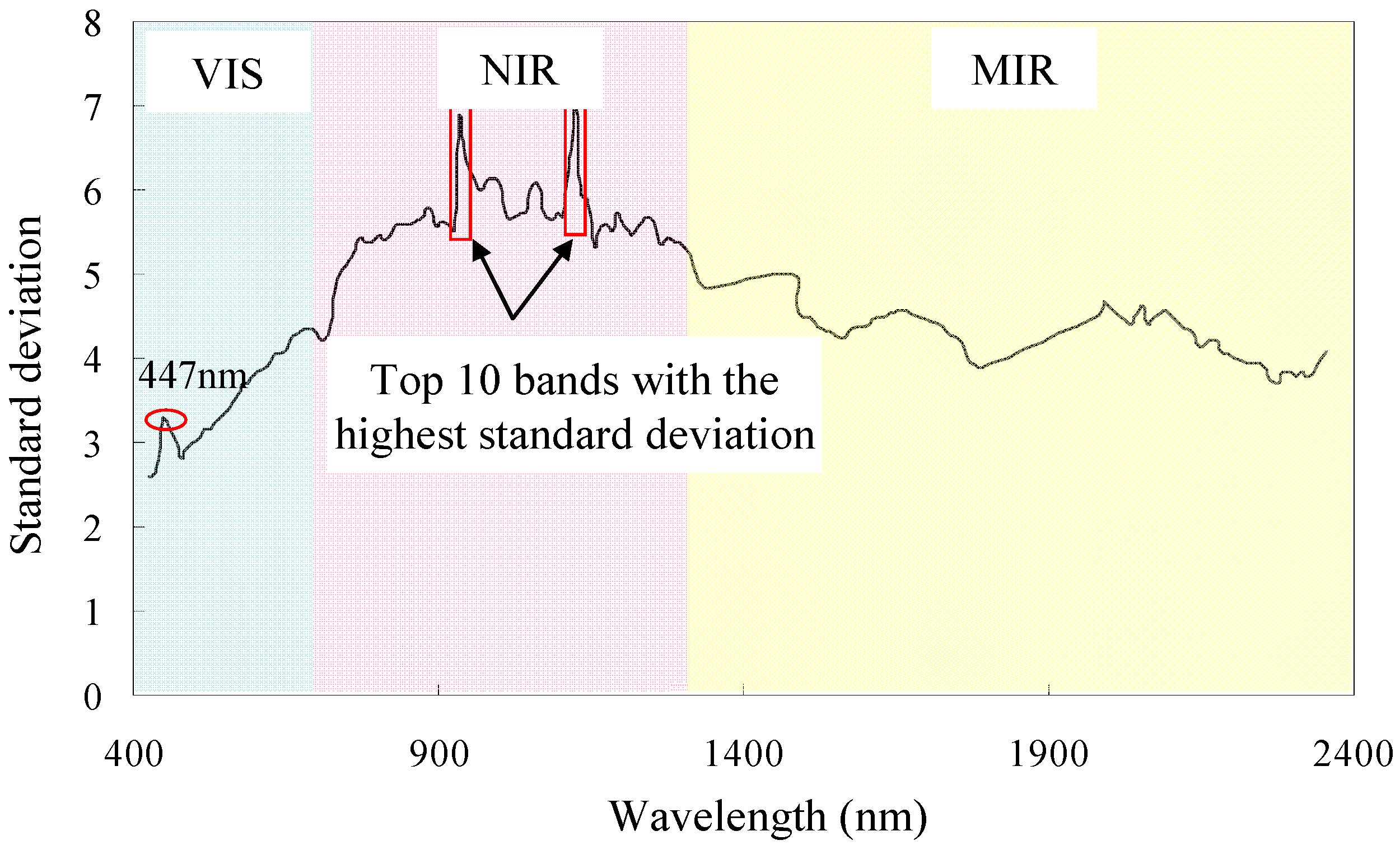
The standard deviations of the bands were selected to evaluate the amount of information contained in each band. A higher standard deviation value indicates higher information content within the band. Figure 3 shows the curve of the change in the standard deviation of the Hyperion image in each band of the Fuzhou image. In general, in the range from visible to near infrared wavelengths, the standard deviation of each band increased with an increasing wavelength. The maximum value occurred in the near infrared band, and the value subsequently began to decline in the mid-infrared band. The wavelength region was further divided into visible light, near infrared and mid-infrared intervals. The standard deviation of each band was ranked in these three intervals, and the top 10 bands with the highest standard deviation in each interval were obtained. In the visible light section, they were 681 nm, 691 nm, 701 nm, 671 nm, 660 nm, 650 nm, 640 nm, 630 nm, 620 nm, and 610 nm. However, Figure 3 shows that the curve of the change in the standard deviation has an obvious peak at 447 nm in the visible light region (indicated by the red circle in Figure 3), which demonstrates that while the standard deviation of the band is not among the top 10, the standard deviation of the image at that wavelength is the highest in the short wave direction. The ranking of the top 10 bands with the highest standard deviations in the near infrared bands were 1124 nm, 932 nm, 942 nm, 1114 nm, 952 nm, 983 nm, 993 nm, 1003 nm, 1053 nm, and 962 nm. The top 10 bands in the mid-infrared bands were those at 1305 nm, 1316 nm, 1477 nm, 1326 nm, 1336 nm, 1991 nm, 1487 nm, 2072 nm, 1699 nm, and 2092 nm.
3.1.3. Correlation Analysis of Hyperion Bands
The correlation coefficient was calculated to evaluate the correlations of the Hyperion bands. A higher correlation coefficient indicates a higher overlapping of the spectral values of two bands, and thus greater similarity between the feature information in those two bands. To obtain more feature information, band combinations with small correlation coefficients must be selected.
Figure 4 shows the correlation coefficient between two of the 158 bands of the Hyperion image. The figure shows that the correlation coefficient matrix between the 158 bands has an obvious block feature. Based on the correlation coefficient, the entire wavelength range is divided into four blocks: Block I: B1–B30 (visible light band, 426–701 nm); Block II: B31–B90 (near infrared band, 711–1306 nm); Block III: B90–B121 (mid-infrared 1 band, 1316–1769 nm); and Block IV: B122–B158 (mid-infrared 2 band, 1780–2355 nm). According to the average correlation coefficient statistics of the bands in the four blocks (Table 2), it was found that the correlation coefficient between the bands was very high within these four blocks, and that the average correlation coefficient was more than 0.95, but the correlation coefficient between the bands in the different blocks was obviously reduced. The average correlation coefficients between Block I and Block II and between Block II and Block IV dropped as low as 0.425 and 0.520, respectively. In the selection of the best feature bands, the appropriate bands must be selected from the four band blocks to ensure that the feature information expressed using the selected bands is the most independent, and that the feature information reflected by the combination of bands is the most comprehensive.
3.1.4. Principal Component Analysis (PCA)
To solve the problems of too many hyperspectral bands and information overlap, PCA is used to reduce the data dimensions. From the statistics of the feature values of each of the PCA components, it was found that the feature values of the first five PCA components accounted for 97.12% of the total original image spectral information. The first and the second principal components accounted for 89.55% of the total. This analysis showed that after PCA, the spectral information contained in the 158 bands had almost all gathered in the first five PCA components, and that PC1 and PC2 were dominant.
Statistics were determined for the contributions of the 158 bands in the Hyperion image in components PC1–5. The top 20 bands, when ranked by their contribution to every PCA component, were listed as shown in Table 3. The table shows that the top 20 bands that make the largest contribution to PC1 are mainly concentrated in the NIR with the wavelength range of 900–1300 nm. In PC2, the ranges of 1900–2350 nm in the MIR2 and 600–700 nm in the red band make the greatest contributions. Because PC1 and PC2 account for 89.55% of the original spectral information and include most of the original image information, the dominant wavelength information in PC1 and PC2 is of major significance when distinguishing between impervious surfaces and pervious surfaces.
3.1.5. Matching of the Best Feature Bands Using Other Analysis Methods
To investigate the reliability of the SDA results, the 11 feature bands selected from the SDA model were compared with the results of the standard deviation, the band correlation, and the PCA.
First, the results of the standard deviation analysis showed that the top 10 bands with the highest standard deviations were at 1124 nm, 932 nm, 942 nm, 1114 nm, 952 nm, 983 nm, 993 nm, 1003 nm, 1053 nm, and 962 nm. The band at 447 nm in the visible light region was the band with the highest standard deviation in the short-wave direction. The bands with the highest standard deviations in the mid-infrared region were at 1305 nm, 1316 nm, 1477 nm, 1326 nm, 1336 nm, 1991 nm, 1487 nm, 2072 nm, 1699 nm, and 2092 nm. There were eight bands with large standard deviations in the discriminant analysis results, comprising those at 447 nm, 942 nm, 1124 nm, 1477 nm, 1487 nm, 1699 nm, 1991 nm, and 2072 nm. This indicated that the 11 feature band combinations that were selected contained most of the image information.
Second, the results of the band correlation analysis showed that the correlation between the bands that were located in different blocks was comparatively small. The 11 selected feature bands were distributed within four blocks. The 447 nm band was in Block I. The 942 nm, 1124 nm, 1154 nm, and 1245 nm bands were in Block II. The 1477 nm, 1487 nm, and 1699 nm bands were in Block III. The 1991 nm, 2072 nm, and 2345 nm bands were in Block IV. Figure 5 shows that the correlation coefficients between pairs of these 11 bands are relatively low. In Figure 5, the blue-green patches with low correlation coefficients account for more than half of the results, and the red patches with high correlation coefficients are basically located on the diagonal that represents the correlation coefficient of each band with itself. Therefore, from the perspective of the correlation analysis, the 11 feature bands that were obtained in the discriminant analysis also have certain reliability.
Third, the PCA results showed that PC1 and PC2 gathered almost 90% of the image spectral information between them, while the NIR and MIR bands were the dominant wavelength ranges in PC1 and PC2, and were also the main bands used for impervious surface information detection. In the results of the discriminant analysis, 447 nm was located in the blue light band, while the remaining 10 bands were all located in the wavelength range from NIR to MIR. After further investigation of the contribution rankings of the bands in the PCA (Table 3), it was found that 10 of the 11 bands made major contributions.
In conclusion, the combination of the 11 feature bands presented here can be used as the best feature band combination to distinguish impervious surfaces from pervious surfaces in the Hyperion image.
The 11 feature bands that were selected from the Fuzhou area were used to synthesize a new image, which was recorded as the Hyperion’. The impervious surface information of the Fuzhou Hyperion image was retrieved using an LSMA model. To verify the effectiveness of this feature band combination and to determine whether it could become the essential band combination required to improve the extraction accuracy of impervious surfaces, the 11 feature bands were also formed in the Hyperion images of Guangzhou and Hangzhou.
3.2. Linear Spectral Mixture Analysis (LSMA)
The principle of the LSMA method is as follows. Assume that the spectrum brightness of a mixed pixel is composed of a linear combination of the basic components of the mixed pixel. These mixed pixel components are known as endmembers. The proportion of each endmember that is contained in the mixed pixel is obtained through calculations, thus allowing us to decompose the spectrum of the mixed pixel into a linear combination of several types of endmembers. The model and its constraint conditions are given as follows [5,21]:
where Rb is the reflectance of the bth band; N is the number of end members; fi is the weight of end member i, representing the ratio of each spectral end member; Rib is the reflectance of end member i in the bth band; and eb is the residual error.
Before the linear spectrum decomposition process, the modified normalized difference water index (MNDWI) [29] was first used to mask the water in each image, thus eliminating the influence of water on the accuracy of the impervious surface extraction. Then, the PCA conversion was completed to reduce the data redundancy. On this basis, the purest spectral pixels were found in the image by calculating the pure pixel index (PPI) [30]. Based on the actual situations in the three areas of interest, four types of endmembers were selected in Fuzhou, Guangzhou, and Hangzhou, comprising high albedo, low albedo, vegetation and soil. Finally, through a linear summation of the high and low albedo components, the impervious surface information was obtained [5,6].
where Rimp,i is the reflectivity of the impervious surface in band i; flow and fhigh are the ratio of low-albedo and high-albedo surface features, respectively; Rlow,i and Rhigh,i are the reflectivity of low-albedo and high-albedo land types in band i, respectively; and ei is the residual error.
Using the above LSMA model, the test images were decomposed, and enhanced images of the impervious surface were then obtained (Figure 6).
3.3. Accuracy Validation
3.3.1. Extraction Accuracy Validation
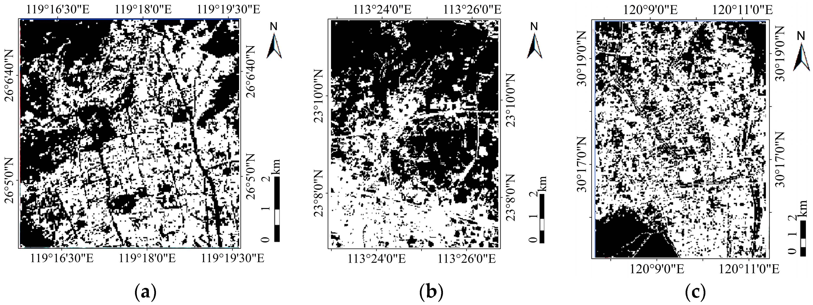
The extraction accuracy is used to determine the degree of consistency of the extracted impervious surface information with the real impervious surface. The impervious surface information was separated from an enhanced image of the impervious surface using a threshold value. As the test areas are all in the metropolitan area with a high-density of buildings, the threshold values are all 60% [31]. Then, the extraction images of the impervious surface were validated using high-resolution images of IKONOS and Google Earth at similar times. Impervious surface extraction images were obtained for the three areas (Figure 7). Before validation, the high-resolution images and the extraction images were overlapped, and then, we collected approximately 300 sample plots using a stratified random sampling method, with 3 × 3 pixels in size, located in purely homogeneous areas, to verify the impervious surface information that was extracted from the three test images. The accuracy validations for soil and vegetation were also implemented for further assessment.
3.3.2. Coverage Accuracy Verification
The coverage accuracy is used to verify any deviation of the impervious surface coverage of each pixel in the enhanced image from the coverage of the real impervious surface.
The root-mean-square error (RMSE), systematic error (SE), and the determination coefficient (R2) were selected as the error indicators for a quantitative evaluation of the validation results. The RMSE is used to measure the overall error of the sample simulation. The SE and R2 are used to measure the system error and the goodness of fit between the simulation and the real coverage values of the impervious surface, respectively.
where Vimodel is the impervious surface coverage of pixel i retrieved by the model, Viactual is the real impervious surface coverage of pixel i, Vmean is the average impervious surface coverage of the validated samples, and N is the number of validated samples, which is 100 in each of the three test areas.
Using the formulas above, the RMSE, SE, and R2 values of the Hyperion images in the three test areas were obtained, and the average impervious surface coverage of 100 sample points was calculated for each image. With the same method, the coverage accuracy validations for soil and vegetation were also implemented for further assessment.
4. Discussion
4.1. Accuracy Evaluation
The enhanced images (Figure 6) and the original images (Figure 1) of the impervious surface were compared. The comparison shows that the impervious surface information that was retrieved from the three test areas is all relatively accurate, and the impervious surfaces are all shown in red and yellow, unlike the pervious surfaces, which are shown in blue and green. This demonstrates that there is less confusion and less missing information when the two images are compared. When we compare Figure 6 with Figure 7, we see that the impervious surface information extracted from the Hyperion images of the three test areas is relatively accurate, and there are fewer errors and fewer missing data.
Furthermore, a quantitative analysis of the extraction accuracy of the impervious surface was carried out. Table 4 shows the accuracy evaluation results of the three test areas. The extraction accuracy for the Fuzhou area is very high, with an overall accuracy of 90.33% and a kappa coefficient of 0.801 (Table 4). In the verification images, the extraction accuracies for Guangzhou and Hangzhou are both more than 88% and the kappa coefficient is above 0.75 in both cases. The impervious surface extraction accuracy in the two verification areas is also relatively high. The accuracies of the soil and the vegetation are also high both in the test area and the verification areas. The overall accuracies and the kappa coefficients are all more than 85% and 0.7, respectively (Table 4). This indicates that when putting the 11 feature bands into the LSMA model, the extraction accuracies of the impervious surface, the soil and the vegetation are all relatively high. Therefore, the three kinds of ground features can be distinguished very well.
The average impervious surface coverage values for Fuzhou, Guangzhou, and Hangzhou are very similar to the real coverage values. The RMSE values and the absolute values of SE of the three areas are all less than 0.1. The R2 is more than 0.8 in all cases (Table 5). This means that the difference between the impervious surface coverage that was retrieved from the three Hyperion images and the real impervious surface coverage is relatively small. Furthermore, the average coverage values of vegetation and soil are also very similar in the three test areas (Table 5). Almost all of the RMSE values of vegetation and soil are less than 0.1; only the RMSE value of vegetation in Hangzhou is 0.106. The absolute values of SE of vegetation and soil in the three test areas are all less than 0.05, and most of the R2 values are more than 0.8. The coverage accuracies of vegetation and soil indicate that when using the 11 feature bands in LSMA model, both the impervious surface and non-impervious surface like vegetation and soil have high coverage accuracies.
4.2. Spectral Analysis of Impervious Surface Extracted Using Hyperion Image
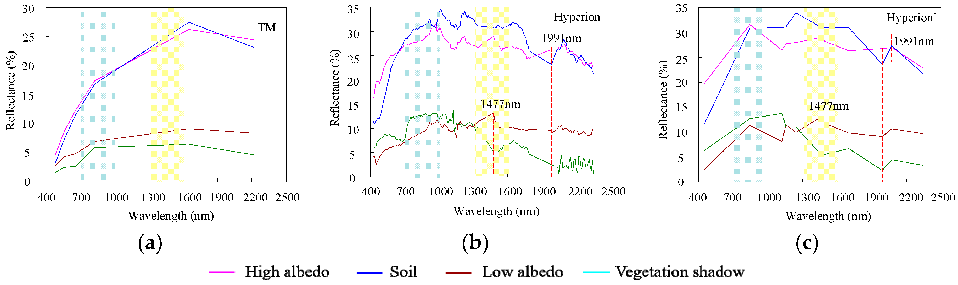
The Hyperion image that was composed of 11 feature bands obtained high impervious surface extraction accuracy. It can distinguish the impervious surface, soil, and vegetation shadow effectively. To better investigate the reason for this, we compared the spectral curves of the Hyperion and multispectral image (i.e., TM). The main reason for the high retrieval accuracy in this study is that the spectral resolution of the Hyperion is greatly improved compared to TM. Within the visible to mid-infrared spectral range, TM only has six bands, while Hyperion has up to 158 effective bands. To investigate the effectiveness of the spectral resolution for impervious surface retrieval, we used the Fuzhou area as an example, and studied the changes in the spectral curves of the different features within the spectral range (Figure 8).
In Figure 8a, the spectral curves of TM are very monotonous, and the up-and-down change is less. The spectral curve of the impervious surface with high albedo almost overlaps together with the soil, and the trend of spectral changes of the impervious surface with low albedo is very similar to vegetation shadow. This may be the important reason why TM images can't differentiate the two groups of ground features.
Conversely, for Hyperion (Figure 8b), because the spectral resolution is greatly improved, the spectral curves of the ground features show large changes, and the impervious surface with high albedo has a low overlap with the soil. In the 700–1000 nm range, the reflectivities of the two components show rising trends, but the impervious surface with high albedo is rising in index terms, while the soil is rising logarithmically. In the 1300–1600 nm range, the reflectivity of the impervious surface with high albedo increases and then decreases, and thus there is a peak. The soil, in contrast, is characterized by a smooth transition. At 1991 nm, the reflectivity of the impervious surface with high albedo rises steadily, but that of the soil shows an obvious valley. The increasing and decreasing aspects of the two curves clearly demonstrate the differences between the spectra of the two different features. However, these differences don’t exist in the TM image. Similarly, for the vegetation shadow and the impervious surface with low albedo, in the TM image (Figure 8a), the two ground features only have one spectral value in the 700–1000 nm range, and they both form a peak. In the 1300–1600 nm range, the spectral curves of the two ground features are both characterized by a smooth transition in TM because TM had no bands setting in this wavelength range. In contrast, in Hyperion (Figure 8b), the vegetation shadow retains the reflection feature of the vegetation. The reflectivity rises steeply within the 700–1000 nm range, and then rises more gently. In the 1300–1600 nm range, the curve shows a valley due to the water vapor absorption band. In contrast, the reflectivity of the impervious surface with low albedo increases approximately linearly over the 700–1000 nm range, and shows a peak near 1000 nm. The curve then falls before increasing, meaning that there is a peak in the curve at 1477 nm.
Only 11 bands in Hyperion’ were selected in this case, but compared to TM (Figure 8a,c), these 11 bands contained all of the essential spectrum differentiators required to distinguish between impervious surfaces with high albedo and soil, and between impervious surfaces with low albedo and vegetation shadow. This also suggests that the 11 bands selected here are effective bands that can distinguish impervious surfaces from other ground features. When compared with the 158 bands of the Hyperion image (Figure 8b,c), these 11 feature bands can improve the ground feature separability, and can also reduce the redundancy between bands, so that the Hyperion’ images composed of the 11 feature bands can display a high impervious surface extraction accuracy. At the same time, the original 158 bands were reduced to 11 bands, and this also greatly diminished the data processing required and reduced the computer processing time.
The endmember is the most important factor in the LSMA model and the spectral separability of endmembers is directly associated with the accuracy of the extracted impervious surface images [5,22,32,33]. A detailed analysis of the PCA results can be used to understand which bands (or groups of bands) were the most important for impervious surface mapping [33]. The PCA analysis of this study found that the near infrared and mid-infrared bands were the dominant wavelengths in impervious surface information detection. It should also be noted that almost all of the feature bands that were selected in this study are in the near infrared and mid-infrared wavelength ranges. We see that the improvement in the spectral resolution of the Hyperion image greatly improves the spectrum separability between easily confused surface features, and also plays an important role in distinguishing soil from impervious surfaces with high albedo, and in distinguishing vegetation shadow from impervious surfaces with low albedo. The analysis above shows that the improvement of the spectral resolution in the near infrared and mid-infrared wavelength ranges is essential to avoid confusion between the impervious surfaces of interest and other surface features. Weng’s study also shows that improvement in the spectral resolution in the mid-infrared band plays an important role in distinguishing ground features with low albedo [33].
Furthermore, there are many studies applying hyperspectral imagery in LSMA to improve the model itself by using special mathematical models [34,35,36] and the hyperspectral imaging has been applied most extensively in the studies of vegetation and water [37,38,39]. In contrast, fewer researches have been applied to impervious surface extraction using hyperspectral images with the LSMA model. The contribution of this study is that we try to find the spectral diversity of impervious surfaces and the spectral requirements for the remote sensing of impervious surfaces. We also proposed a combination of 11 feature bands and applied them in the LSMA model to distinguish the impervious surface from the other ground features, and the extraction results are relatively accurate.
5. Conclusions
In this study, 11 feature bands that could distinguish the impervious surface from the other ground features were determined from the Hyperion image with 158 bands using the SDA method. The standard deviations in each band of the Hyperion image and the correlations between the bands were analyzed. PCA was also completed in all 158 bands to select feature bands. The 11 feature band combination that was suitable for impervious surface extraction from hyperspectral images was then proposed. These 11 feature bands were synthetized into new Hyperion images, and impervious surface extraction tests were conducted in the Fuzhou, Guangzhou, and Hangzhou test area images. The results show that the impervious surfaces that were extracted from the three test areas are both accurate and reliable. Therefore, the 11 feature bands that were obtained in this study have good universality. The impervious surface information extraction accuracy is high when this feature band combination is used, and it does not vary for different areas. The method used here is expected to be widely applied to impervious surface information extraction.
Our result suggests that the Hyperion image was very effective for identifying the impervious surface. The improvement in mapping accuracy in general and the better ability to discriminate the impervious surface came mainly from additional bands in the midinfrared. The problem of confusion among the impervious surface, soil, and vegetation shadow can be improved with the help of hyperspectral remote sensing images, but currently, hyperspectral remote sensing images are very limited [40], so it is hard to completely solve the problem by relying on hyperspectral data. Further research is suggested in the following areas: (1) as the texture and the geometry of the bare soil and vegetation are very different from the impervious surfaces such as roads, buildings, and parking lots, using the effective auxiliary texture of features to classify the impervious surface and the others is expected to improve the accuracy; (2) different methods may be used to remove shades from satellite imagery, which tend to be confused with low-albedo materials; (3) with the popularity of LiDAR data, impervious surface estimation and mapping should use the elevation data of LiDAR remote sensing images to distinguish buildings and soil [41,42].
Acknowledgments
This study is supported by the National Natural Science Foundation of China (No. 41501469).
Author Contributions
Hanqiu Xu and Fei Tang conceived and designed the experiments; Fei Tang performed the experiments, analyzed the data, and wrote the paper; Hanqiu Xu reviewed and commented on the manuscript.
Conflicts of Interest
The authors declare no conflict of interest.
References
- Gillies, R.; Box, J.; Symanzik, J.; Rodemaker, E. Effects of urbanization on the aquatic fauna of the Line Creek watershed, Atlanta—A satellite perspective. Remote Sens. Environ. 2003, 86, 411–422. [Google Scholar] [CrossRef]
- Yang, L.; Huang, C.; Homer, C.; Wylie, B.; Coan, M. An approach for mapping large-area impervious surfaces: Synergistic use of Landsat-7 ETM+ and high spatial resolution imagery. Can. J. Remote Sens. 2003, 29, 230–240. [Google Scholar] [CrossRef]
- Weng, Q. Remote sensing of impervious surfaces in the urban areas: Requirements, methods, and trends. Remote Sens. Environ. 2012, 117, 34–49. [Google Scholar] [CrossRef]
- Ji, M.; Jensen, J.R. Effectiveness of subpixel analysis in detecting and quantifying urban imperviousness from Landsat Thematic Mapper imagery. Geocarto Int. 1999, 14, 33–41. [Google Scholar] [CrossRef]
- Wu, C.; Murray, A.T. Estimating Impervious Surface Distribution by Spectral Mixture Analysis. Remote Sens. Environ. 2003, 84, 493–505. [Google Scholar] [CrossRef]
- Xu, H.Q. Analysis of impervious surface and its impact on urban heat environment using the normalized difference impervious surface index (NDISI). Photogramm. Eng. Remote Sens. 2010, 76, 557–565. [Google Scholar] [CrossRef]
- Deng, C.B.; Wu, C.S. BCI: A biophysical composition index for remote sensing of urban environments. Remote Sens. Environ. 2012, 127, 247–259. [Google Scholar] [CrossRef]
- Ma, Y.; Kuang, Y.Q.; Huang, N.S. Coupling urbanization analyses for studying urban thermal environment and its interplay with biophysical parameters based on TM/ETM+ imagery. Int. J. Appl. Earth Obs. Geoinf. 2010, 12, 110–118. [Google Scholar] [CrossRef]
- Carlson, T.N.; Arthur, S.T. The impact of land use—land cover changes due to urbanization on surface microclimate and hydrology: A satellite perspective. Glob. Planet. Chang. 2000, 25, 49–65. [Google Scholar] [CrossRef]
- Shao, Y.; Li, G.L.; Guenther, E.; Campbell, J.B. Evaluation of topographic correction on subpixel impervious cover mapping with CBERS-2B data. IEEE Geosci. Remote Sens. Lett. 2015, 12, 1675–1679. [Google Scholar] [CrossRef]
- Lu, D.S.; Hetrick, S.; Moran, E. Impervious surface mapping with Quickbird imagery. Int. J. Remote Sens. 2011, 32, 2519–2533. [Google Scholar] [CrossRef] [PubMed]
- Xu, H.Q. Rule-based impervious surface mapping using high spatial resolution imagery. Int. J. Remote Sens. 2013, 34, 27–44. [Google Scholar] [CrossRef]
- Durbha, S.S.; King, R.L.; Younan, N.H. Support vector machines regression for retrieval of leaf area index from multiangle imaging spectroradiometer. Remote Sens. Environ. 2007, 107, 348–361. [Google Scholar] [CrossRef]
- Okujeni, A.; van der Linden, S.; Hostert, P. Extending the vegetation–impervious–soil model using simulated EnMAP data and machine learning. Remote Sens. Environ. 2015, 158, 69–80. [Google Scholar] [CrossRef]
- Van de Voorde, T.; De Roeck, T.; Canters, F. A comparison of two spectral mixture modelling approaches for impervious surface mapping in urban areas. Int. J. Remote Sens. 2009, 30, 4785–4806. [Google Scholar] [CrossRef]
- Yuan, F.; Bauer, M.E. Mapping impervious surface area using high resolution imagery: A comparison of object-based and per pixel classification. In Proceedings of the American Society for Photogrammetry and Remote Sensing 2006 Annual Conference, Reno, NV, USA, 1 May 2006. [Google Scholar]
- Hu, X.F.; Weng, Q.H. Impervious surface area extraction from IKONOS imagery using an object-based fuzzy method. Geocarto Int. 2011, 26, 3–20. [Google Scholar] [CrossRef]
- Weng, Q.H.; Hu, X.F. Medium spatial resolution satellite imagery for estimating and mapping urban impervious surfaces using LSMA and ANN. IEEE Trans. Geosci. Remote Sens. 2008, 46, 2397–2406. [Google Scholar] [CrossRef]
- Pu, R.L.; Gong, P.; Michishita, R.; Sasagawa, T. Spectral mixture analysis for mapping abundance of urban surface components from the Terra/ASTER data. Remote Sens. Environ. 2008, 112, 939–954. [Google Scholar] [CrossRef]
- Ridd, M.K. Exploring a V-I-S (vegetation-impervious surface-soil) Model for Urban Ecosystem Analysis through Remote Sensing: Comparative Anatomy for Cities. Int. J. Remote Sens. 1995, 16, 2165–2185. [Google Scholar] [CrossRef]
- Wu, C. Normalized spectral mixture analysis for monitoring urban composition using ETM+ imagery. Remote Sens. Environ. 2004, 93, 480–492. [Google Scholar] [CrossRef]
- Powell, S.L.; Cohen, W.B.; Yang, Z.; Pierce, J.D.; Alberti, M. Quantification of impervious surface in the Snohomish Water Resources Inventory Area of western Washington from 1972–2006. Remote Sens. Environ. 2008, 112, 1895–1908. [Google Scholar] [CrossRef]
- Yang, F.; Matsushita, B.; Fukushima, T. A pre-screened and normalized multiple endmember spectral mixture analysis for mapping impervious surface area in Lake Kasumigaura Basin, Japan. ISPRS J. Photogramm. Remote Sens. 2010, 65, 479–490. [Google Scholar] [CrossRef]
- Lu, D.; Moran, E.; Hetrick, S. Detection of impervious surface change with multitemporal Landsat images in an urban-rural frontier. ISPRS J. Photogramm. Remote Sens. 2011, 66, 298–306. [Google Scholar] [CrossRef] [PubMed]
- Zhou, C.; Xu, H. A Spectral Mixture Analysis and Mapping of Impervious Surfaces in Built-up Land of Fuzhou City. J. Image Graph. 2007, 12, 875–881. [Google Scholar]
- Zhao, X.; Qiu, Q. A Comparative Study of Four Spectral Mixture Analysis Methods for Land Surface Composition in a Hilly Coastal City. Remote Sens. Technol. Appl. 2009, 24, 737–742. [Google Scholar]
- Li, B.; Huang, J.; Wu, C. Estimating Urban Impervious Surface Based on Thermal Infrared Remote Sensing Data and a Spectral Mixture Analysis Model. J. Nat. Res. 2012, 27, 1590–1600. [Google Scholar]
- SAS Institute. SAS/STAT(R) 9.2 User's Guide, Second Edition; SAS Institute: Cary, NC, USA, 2008. [Google Scholar]
- Xu, H.Q. Modification of Normalized Difference Water Index (NDWI) to Enhance Open Water Features in Remotely Sensed Imagery. Int. J. Remote Sens. 2006, 27, 3025–3033. [Google Scholar] [CrossRef]
- Boardman, J.W.; Kruse, F.A.; Green, R.O. Mapping target signatures via partial unmixing of AVIRIS data. In Proceedings of the Fifth JPL Airborne Earth Science Workshop, Pasadena, CA, USA, 23–26 January 1995. [Google Scholar]
- Xian, G.; Crane, M. An analysis of urban thermal characteristics and associated land cover in Tampa Bay and Las Vegas using Landsat satellite data. Remote Sens. Environ. 2006, 104, 147–156. [Google Scholar] [CrossRef]
- Tang, F.; Xu, H.Q. Comparison of performances in retrieving impervious surface between Hyperspectral (Hyperion) and multispectral (TM/ETM+) images. Spectrosc. Spectr. Anal. 2014, 34, 1075–1080. [Google Scholar]
- Weng, Q.; Hu, X.; Lu, D. Extracting impervious surfaces from medium spatial resolution multispectral and hyperspectral imagery: A comparison. Int. J. Remote Sens. 2008, 29, 3209–3232. [Google Scholar] [CrossRef]
- Chang, C.I.; Chiang, S.S.; Smith, J.A.; Ginsberg, I.W. Linear spectral random mixture analysis for hyperspectral imagery. IEEE Trans. Geosci. Remote Sens. 2002, 40, 375–392. [Google Scholar] [CrossRef]
- Nielsen, A.A. Spectral Mixture Analysis: Linear and Semi-parametric Full and Iterated Partial Unmixing in Multi- and Hyperspectral Image Data. Int. J. Comput. Vis. 2001, 42, 17–37. [Google Scholar] [CrossRef]
- Dobigeon, N.; Altmann, Y.; Brun, N.; Moussaoui, S. Linear and nonlinear unmixing in Hyperspectral imaging (Chapter 6). Data Handl. Sci. Technol. 2016, 30, 185–224. [Google Scholar]
- Thenkabail, P.S.; Enclona, E.A.; Ashton, M.S.; Van Der Meer, B. Accuracy assessments of hyperspectral waveband performance for vegetation analysis applications. Remote Sens. Environ. 2004, 91, 354–376. [Google Scholar] [CrossRef]
- Wu, D.H.; Fan, W.J.; Cui, Y.K.; Yan, B.Y.; Xu, X.R. Review of monitoring soil water content using hyperspectral remote sensing. Spectrosc. Spectr. Anal. 2010, 30, 3067–3071. [Google Scholar]
- Guerschman, J.P.; Hill, M.J.; Renzullo, L.J.; Barrett, D.J.; Marks, A.S.; Botha, E.J. Estimating fractional cover of photosynthetic vegetation, non-photosynthetic vegetation and bare soil in the Australian tropical savanna region upscaling the EO-1 Hyperion and MODIS sensors. Remote Sens. Environ. 2009, 113, 928–945. [Google Scholar] [CrossRef]
- Xu, H.Q.; Wang, M.Y. Remote sensing-based retrieval of ground impervious surfaces. J. Remote Sens. 2016, 20, 1270–1289. [Google Scholar]
- Parent, J.R.; Volin, J.C.; Civco, D.L. A fully-automated approach to land cover mapping with airborne LiDAR and high resolution multispectral imagery in a forested suburban landscape. ISPRS J. Photogramm. Remote Sens. 2015, 104, 18–29. [Google Scholar] [CrossRef]
- Singh, K.K.; Vogler, J.B.; Shoemaker, D.A.; Meentemeyer, R.K. LiDAR-Landsat data fusion for large-area assessment of urban land cover: Balancing spatial resolution, data volume and mapping accuracy. ISPRS J. Photogramm. Remote Sens. 2012, 74, 110–121. [Google Scholar] [CrossRef]
Figure 1.
Original images (RGB: Hyperion: 41, 24, 14): (a) Fuzhou; (b) Guangzhou; (c) Hangzhou.
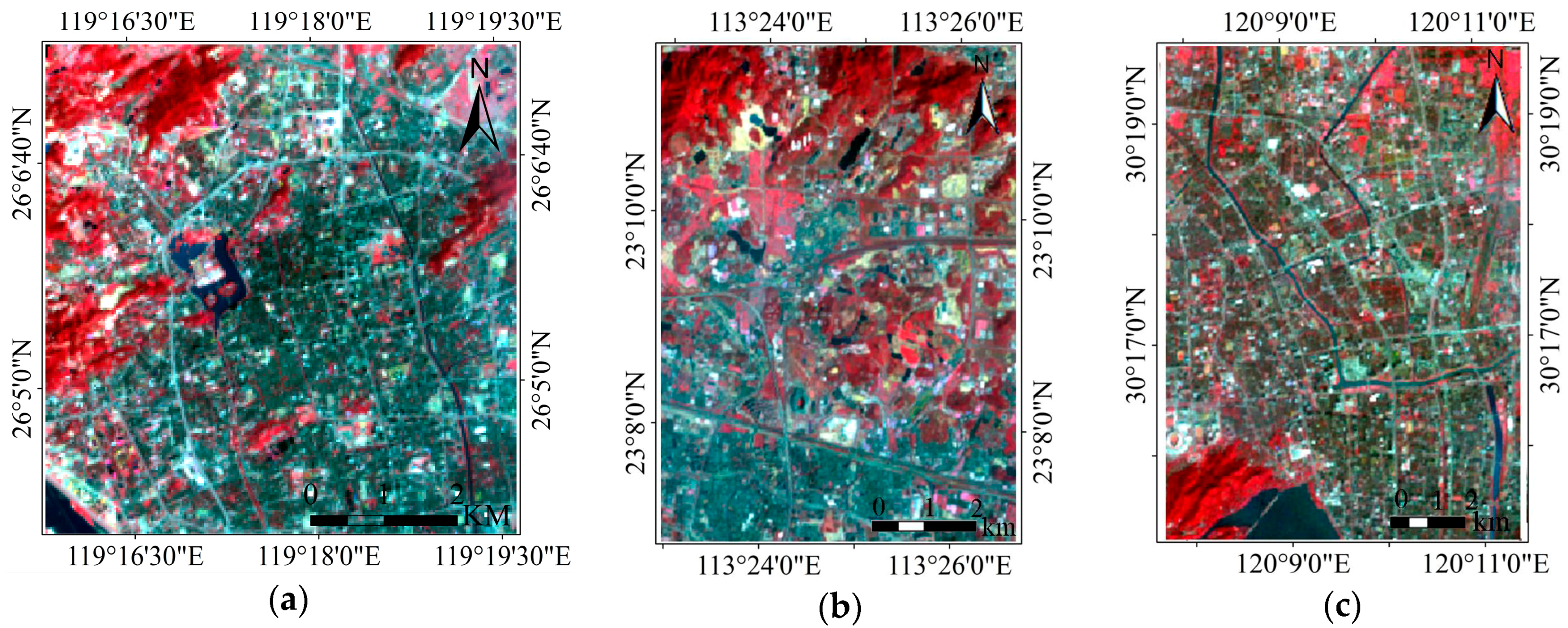
Figure 2.
Flow chart of the stepwise discriminant analysis (SDA) process.
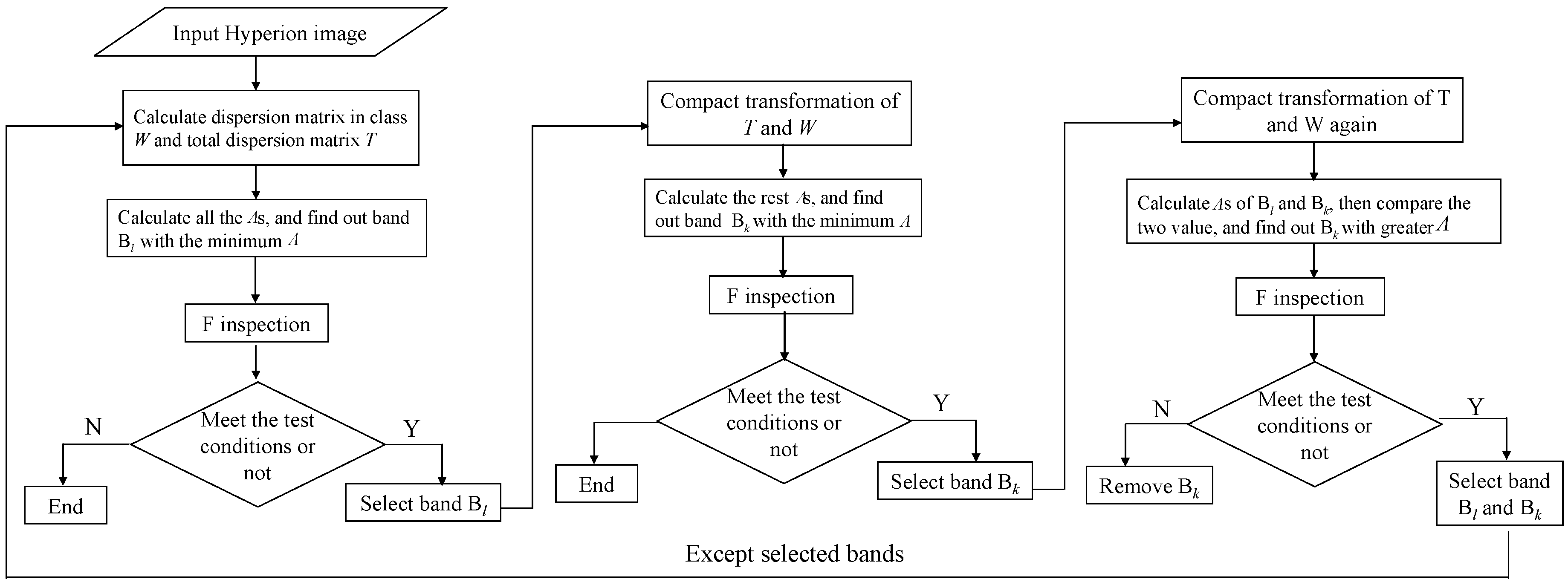
Figure 3.
Standard deviation of each band in the Hyperion image: the wavelength is divided into three internals as VIS, NIR, and MIR. The top 10 bands with the highest standard deviation are in the NIR.
Figure 3.
Standard deviation of each band in the Hyperion image: the wavelength is divided into three internals as VIS, NIR, and MIR. The top 10 bands with the highest standard deviation are in the NIR.

Figure 4.
Correlation coefficient matrixes of the Hyperion bands: the entire wavelength range is divided into four blocks: Block I: B1–B30 (visible light band, 426–701 nm); Block II: B31–B90 (near infrared band, 711–1306 nm); Block III: B90–B121 (mid-infrared 1 band, 1316–1769 nm); and Block IV: B122–B158 (mid-infrared 2 band, 1780–2355 nm).
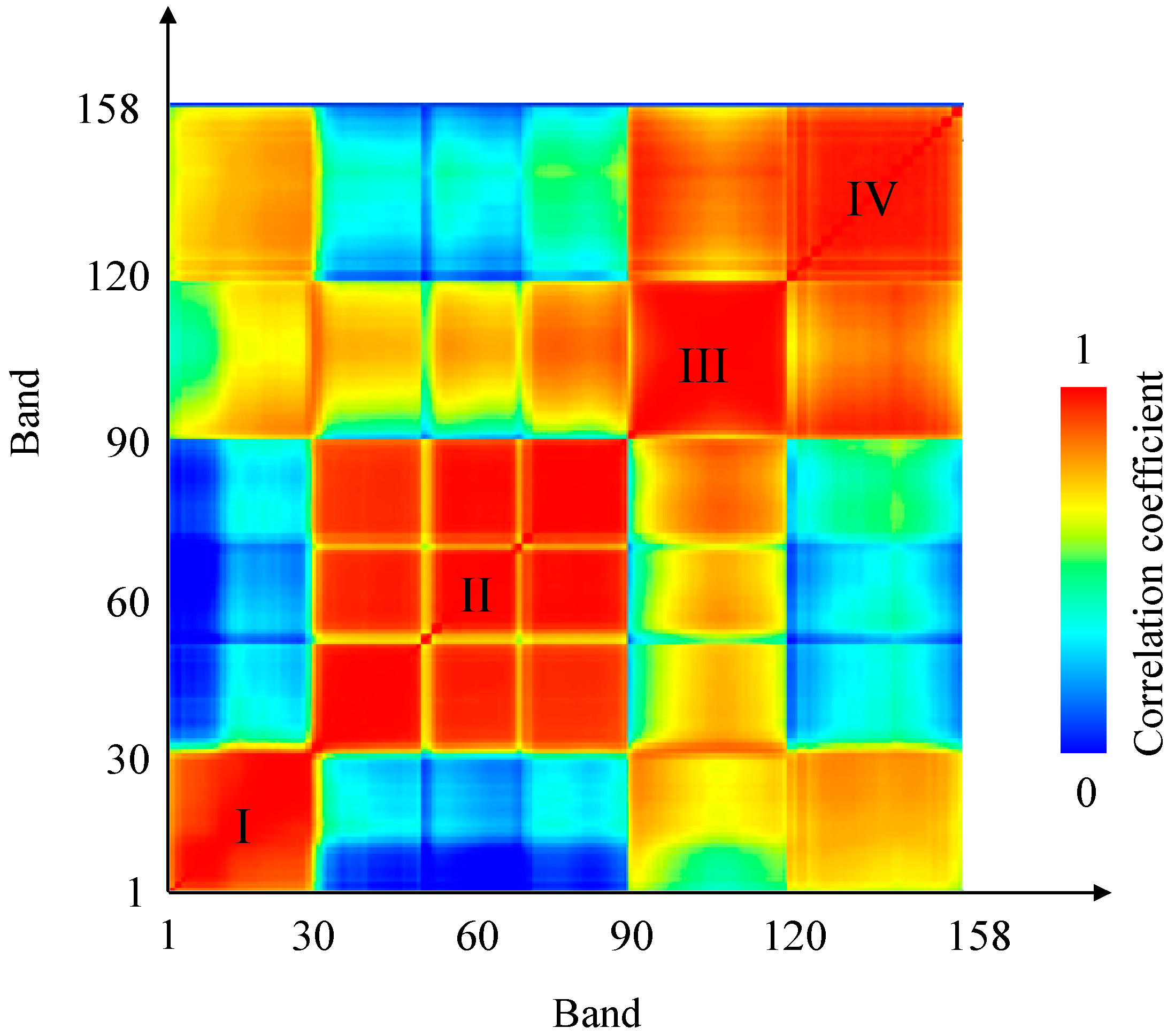
Figure 5.
Correlation coefficient matrixes of the 11 selected feature bands.
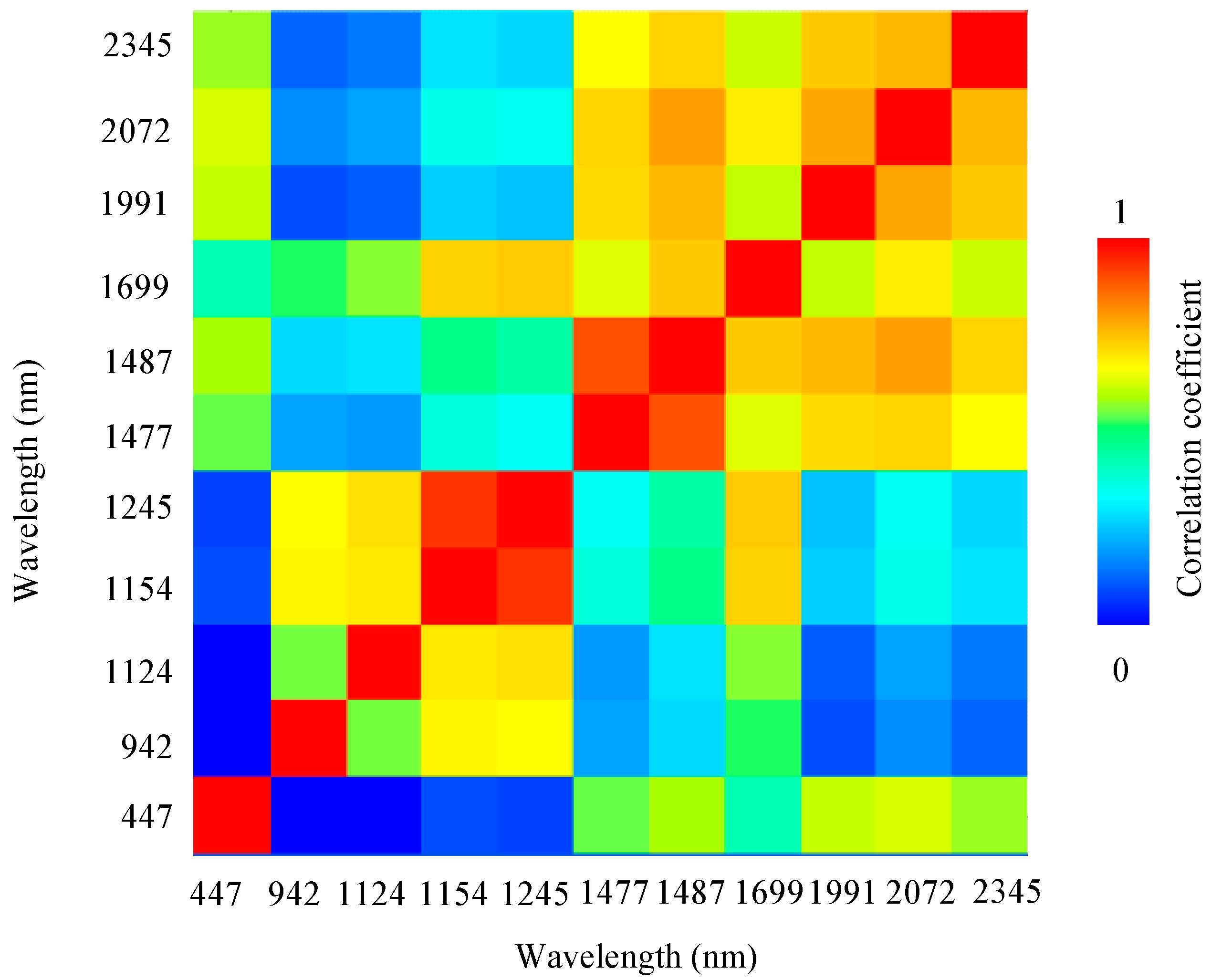
Figure 6.
Enhanced images of the impervious surface: (a) Fuzhou; (b) Guangzhou; (c) Hangzhou.
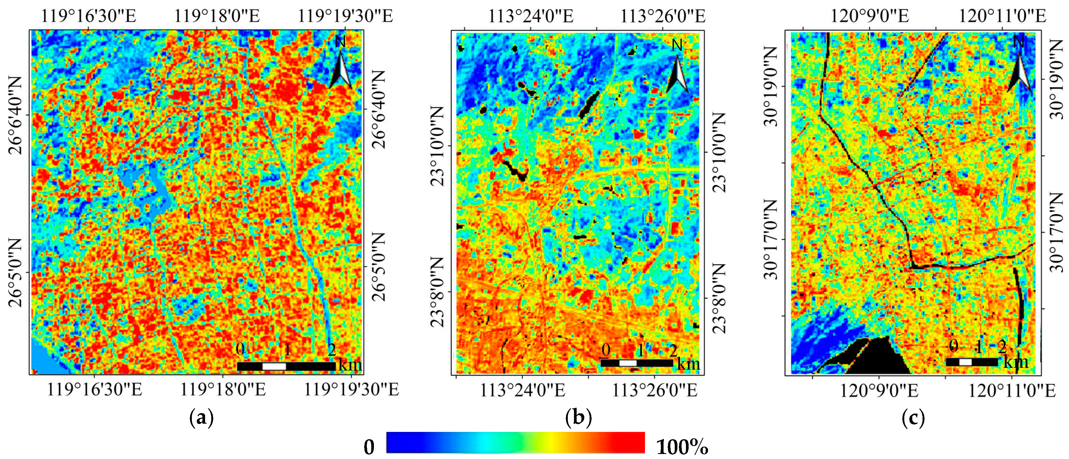
Figure 7.
Extraction images of impervious surface: (a) Fuzhou; (b) Guangzhou; (c) Hangzhou; The area with white color is the impervious surface.
Figure 7.
Extraction images of impervious surface: (a) Fuzhou; (b) Guangzhou; (c) Hangzhou; The area with white color is the impervious surface.

Figure 8.
Signature of the main endmembers (Fuzhou case): (a) Spectral curves of TM image; (b) Spectral curves of Hyperion image; and (c) Spectral curves of Hyperion’ image.
Figure 8.
Signature of the main endmembers (Fuzhou case): (a) Spectral curves of TM image; (b) Spectral curves of Hyperion image; and (c) Spectral curves of Hyperion’ image.


Table 1.
The parameters of the images used in the study.
| Sensors | Area | Date | Number of Bands | Spatial Resolution | Use |
|---|---|---|---|---|---|
| Hyperion | Fuzhou | 26 March 2003 | 242 | 30 m | Feature bands selection |
| Hangzhou | 2 November 2002 | 242 | 30 m | Model validation | |
| Guangzhou | 5 March 2008 | 242 | 30 m | ||
| IKONOS | Fuzhou | 22 June 2003 | 4 | 4 m | Accuracy validation |
| Google Earth | Hangzhou | 26 September 2002 | 3 | 4 m | |
| Guangzhou | 26 July 2008 | 3 | 4 m |
Table 2.
Average correlation coefficient statistics between the band blocks.
| Block I | Block II | Block III | Block IV | |
|---|---|---|---|---|
| Block I | 0.956 | |||
| Block II | 0.425 | 0.956 | ||
| Block III | 0.737 | 0.778 | 0.974 | |
| Block IV | 0.816 | 0.520 | 0.885 | 0.957 |
Table 3.
Bands making the largest contributions to PC1—PC5.
| PCA Bands | Wavelength (nm) | Dominant Bands |
|---|---|---|
| PC1 | 983, 993, 1124, 1003, 972, 1053, 1114, 962, 1063, 1194, 1245, 952, 1144, 1174, 1205, 1235, 884, 942, 1154, 1225 | NIR |
| PC2 | 1981, 1991, 2042, 2052, 2032, 2072, 2082, 2092, 2062, 681, 671, 1477, 2102, 691, 660, 2113, 2123, 2133, 650, 2345 | MIR2, Red |
| PC3 | 1991, 1981, 2042, 2052, 2032, 2193, 2203, 2355, 2183, 2345, 2062, 2072, 2213, 2224, 2082, 2092, 2173, 2234, 2163, 2314 | MIR2 |
| PC4 | 932, 942, 952, 1477, 962, 1981, 1487, 1991, 447, 457, 487, 467, 498, 508, 477, 518, 436, 2345, 528, 2072 | NIR, MIR1, Blue, Green, MIR2 |
| PC5 | 1124, 1114, 681, 671, 660, 691, 650, 1134, 630, 640, 1144, 620, 610, 599, 589, 579, 701, 1194, 1245, 1205 | Green, Red, NIR |
Table 4.
Extraction accuracy of the impervious surface information, soil, and vegetation.
| Ground Types | Area | Fuzhou | Guangzhou | Hangzhou |
|---|---|---|---|---|
| Impervious surface | Overall accuracy | 90.33% | 88.33% | 88.00% |
| Kappa | 0.801 | 0.761 | 0.753 | |
| Soil | Overall accuracy | 89.20% | 88.27% | 85.11% |
| Kappa | 0.782 | 0.757 | 0.721 | |
| Vegetation | Overall accuracy | 90.80% | 86.65% | 85.37% |
| Kappa | 0.807 | 0.736 | 0.725 |
Table 5.
Coverage accuracy of the impervious surfaces, vegetation and soil.
| Area | Ground Types | Image Pairs | Average | RMSE | SE | R2 |
|---|---|---|---|---|---|---|
| Fuzhou | Impervious surface | Hyperion | 0.645 | 0.099 | −0.024 | 0.800 |
| IKONOS | 0.668 | / | / | / | ||
| Vegetation | Hyperion | 0.398 | 0.006 | 0.021 | 0.845 | |
| IKONOS | 0.377 | / | / | / | ||
| Soil | Hyperion | 0.107 | 0.003 | 0.011 | 0.890 | |
| IKONOS | 0.096 | / | / | / | ||
| Guangzhou | Impervious surface | Hyperion | 0.579 | 0.077 | −0.016 | 0.881 |
| Google Earth | 0.595 | / | / | / | ||
| Vegetation | Hyperion | 0.434 | 0.086 | 0.013 | 0.816 | |
| Google Earth | 0.421 | / | / | / | ||
| Soil | Hyperion | 0.187 | 0.005 | 0.008 | 0.853 | |
| Google Earth | 0.179 | / | / | / | ||
| Hangzhou | Impervious surface | Hyperion | 0.662 | 0.089 | −0.034 | 0.894 |
| Google Earth | 0.696 | / | / | / | ||
| Vegetation | Hyperion | 0.375 | 0.106 | 0.022 | 0.769 | |
| Google Earth | 0.353 | / | / | / | ||
| Soil | Hyperion | 0.086 | 0.098 | 0.013 | 0.802 | |
| Google Earth | 0.073 | / | / | / |
© 2017 by the authors. Licensee MDPI, Basel, Switzerland. This article is an open access article distributed under the terms and conditions of the Creative Commons Attribution (CC BY) license (http://creativecommons.org/licenses/by/4.0/).
Share and Cite
MDPI and ACS Style
Tang, F.; Xu, H. Impervious Surface Information Extraction Based on Hyperspectral Remote Sensing Imagery. Remote Sens. 2017, 9, 550. https://doi.org/10.3390/rs9060550
AMA Style
Tang F, Xu H. Impervious Surface Information Extraction Based on Hyperspectral Remote Sensing Imagery. Remote Sensing. 2017; 9(6):550. https://doi.org/10.3390/rs9060550
Chicago/Turabian StyleTang, Fei, and Hanqiu Xu. 2017. "Impervious Surface Information Extraction Based on Hyperspectral Remote Sensing Imagery" Remote Sensing 9, no. 6: 550. https://doi.org/10.3390/rs9060550
Note that from the first issue of 2016, this journal uses article numbers instead of page numbers. See further details here.