
Validation of Sentinel-1A SAR Coastal Wind Speeds Against Scanning LiDAR


DTU Wind Energy, Roskilde 4000, Denmark
*
Author to whom correspondence should be addressed.
Remote Sens. 2017, 9(6), 552; https://doi.org/10.3390/rs9060552
Submission received: 20 April 2017
/
Revised: 18 May 2017
/
Accepted: 26 May 2017
/
Published: 2 June 2017
(This article belongs to the Special Issue Calibration and Validation of Synthetic Aperture Radar)
Abstract
:High-accuracy wind data for coastal regions is needed today, e.g., for the assessment of wind resources. Synthetic Aperture Radar (SAR) is the only satellite borne sensor that has enough resolution to resolve wind speeds closer than 10 km to shore but the Geophysical Model Functions (GMF) used for SAR wind retrieval are not fully validated here. Ground based scanning light detection and ranging (LiDAR) offer high horizontal resolution wind velocity measurements with high accuracy, also in the coastal zone. This study, for the first time, examines accuracies of SAR wind retrievals at 10 m height with respect to the distance to shore by validation against scanning LiDARs. Comparison of 15 Sentinel-1A wind retrievals using the GMF called C-band model 5.N (CMOD5.N) versus LiDARs show good agreement. It is found, when nondimenionalising with a reference point, that wind speed reductions are between 4% and 8% from 3 km to 1 km from shore. Findings indicate that SAR wind retrievals give reliable wind speed measurements as close as 1 km to the shore. Comparisons of SAR winds versus two different LiDAR configurations yield root mean square error (RMSE) of 1.31 and 1.42 for spatially averaged wind speeds.
1. Introduction
Synthetic Aperture Radar (SAR) systems are remote sensing devices that measure radar backscatter signals from the Earth’s surface to infer geophysical parameters. Over the ocean they receive backscatter primarily from centimeter-scale Bragg waves. These small scale waves react quickly to changes of the wind speed and render measurements suitable to infer wind speeds. The backscatter signal is linked to a wind speed via Geophysical Model Functions (GMF) that are tuned to give winds at 10 m height as an output, see Dagestad et al. [1] for an overview and state of the art references. Most GMFs, including the C-band model (CMOD) family, are developed for scatterometers but application for SAR systems is also possible. Satellite SAR winds are typically retrieved with pixel sizes on the order of 0.5–1 km over image swaths up to several hundred kilometers wide. SAR wind fields at those resolutions will represent the spatial variability of the wind [2]. Therefore, these measurements are very suited for applications that need high spatial resolution over a large area, e.g., assessment of wind resources necessary before building offshore wind farms.
Space borne SAR systems have been operational since the 1990s. The archive of SAR images is growing fast, especially since the recent launch of the Sentinel-1 mission by the European Space Agency, and updated GMFs have improved the wind retrievals over the years [3,4,5]. Most data utilized to develop GMFs is available on the open ocean from ocean buoys and model data. GMFs today are based on empirical fits to these data. Additional to wind, many other factors can influence small scale waves on the ocean surface that are not accounted for in of the GMF. For example biological or oil slicks dampen Bragg waves [6], ocean currents locally change wave fields, and the bathymetry [7] also influences the radar backscatter (for an overview, see Christiansen et al. [8]). The influence of those effects can change when moving from the open ocean to the coastal zone.
Table 1 shows an overview of selected past studies validating C-band SAR winds in coastal regions using meteorological masts [9,10,11,12,13,14,15,16]. Resulting Root Mean Square Errors (RMSE) ranged between 0.64 and 2.34 . These RMSEs are comparable to results from validation studies in the open ocean using buoy data, scatterometer derived winds, atmospheric modelling [5,17,18,19] that ranged between 0.65 and 1.76 . Large influences of the wind directions from land or from the sea with high RMSEs above 2 were found in Takeyama et al. [13] and Takeyama et al. [11] while very little influence was found in Chang et al. [10]. Validation studies for coastal sites in Table 1 were done with point measurements from meteorological masts and indicate that SAR can measure wind speeds in the coastal zone. Nonetheless, such studies are based on single point in situ observations for the validation. This does not allow for an estimation of the dependency of SAR wind retrievals to the distance from the coast. In addition, the coastal gradient—manifested as a reduction of wind speed when approaching the coastline from offshore—has not been validated from SAR retrievals.
Accurate wind speed measurements from ground based Light Detection and Ranging (LiDAR) have been available for some time. A laser emits a coherent infrared pulse and receives the backscatter from small aerosols following the air flow. Due to the wind velocity in the direction of the laser beam, the received signal has a Doppler shift and the line of sight wind speed can be determined [20,21]. LiDAR measurements are of high accuracy compared with well established measurements from meteorological masts [20,22,23]. Recently, scanning LiDARs with ranges up to 8 km and the ability to coordinate their scanning patterns became available [24]. Scanning LiDARs offer a combination of high accuracy and good spatial resolution [25]. Therefore, scanning LiDAR measurements can be used to validate the ability of SAR wind retrievals to estimate the coastal wind speed gradient. LiDARs also offer high spatial and temporal resolution but need to be deployed in the area of interest while space borne SAR can measure without locally installing equipment but with the disadvantage of low temporal resolution depending on satellite overpasses. Both measurement techniques are promising in their ability to study the flow in coastal areas.
Assessment of wind resources for the installation of offshore wind farms needs accurate information on the wind speed. Most wind farms are placed within 50 km off the coast where the marine boundary layer can still be affected by the coast [26]. Scatterometer and SAR retrieved winds in combination are used for wind resource assessment, e.g., over the Great Lakes [27] and Northern Europe [9,28]. High resolution wind speed measurements from SAR can show the coastal horizontal wind speed gradient and validation of this ability will e.g., increase the value of SAR measurements for wind resource assessment.
SAR is the only sensor in space that can retrieve wind speeds as close as a couple of hundred meters to the coast but the dependency of the wind retrieval accuracies on the distance to shore is unknown. Several studies have performed validations on single point measurements where the RMSE varies and is mostly below 2 . A study to validate SAR wind retrievals in the coastal zone towards their ability to spatially resolve the wind gradient is missing. This study aims to bridge the validation gap between offshore and coastal SAR retrievals by comparing SAR wind retrievals and scanning LiDAR measurements for one coastal site. Additionally, a method is presented to compare SAR wind retrievals and scanning LiDARs, taking into account intrinsic differences between the wind speed measurement of both systems.
This study investigates the performance of SAR wind retrievals from Sentinel-1A for the first 5 km from the coast line. Comparisons are made using scanning LiDARs—a ground based remote sensing device for wind speed measurements that has recently become available. During the measurement campaign “Reducing uncertainty of near-shore wind resource estimates using onshore LiDAR” (RUNE), offshore wind speeds were measured from the shoreline up to 5 km offshore [29]. This unique LiDAR dataset offers an opportunity to examine the validity and accuracy of SAR wind retrievals in the coastal zone. LiDAR observations have been previously compared with SAR wind retrievals but for an offshore region in the North Sea far from land [30]. The novelty of the current study is the comparisons of SAR wind retrievals with reliable reference measurements for multiple distances from the shore line. It is possible to determine if the accuracy of SAR wind retrievals has a significant dependency on the distance to shore for the first few kilometers in the same study area. Furthermore, it is possible to determine if SAR winds can represent the typical reduction of wind speeds when approaching the coast. Such a validation study will help to utilize the full potential of SAR, e.g., for offshore wind farm installation, by providing information on the validity of coastal wind speed gradient measurements from SAR systems.
2. Materials and Methods
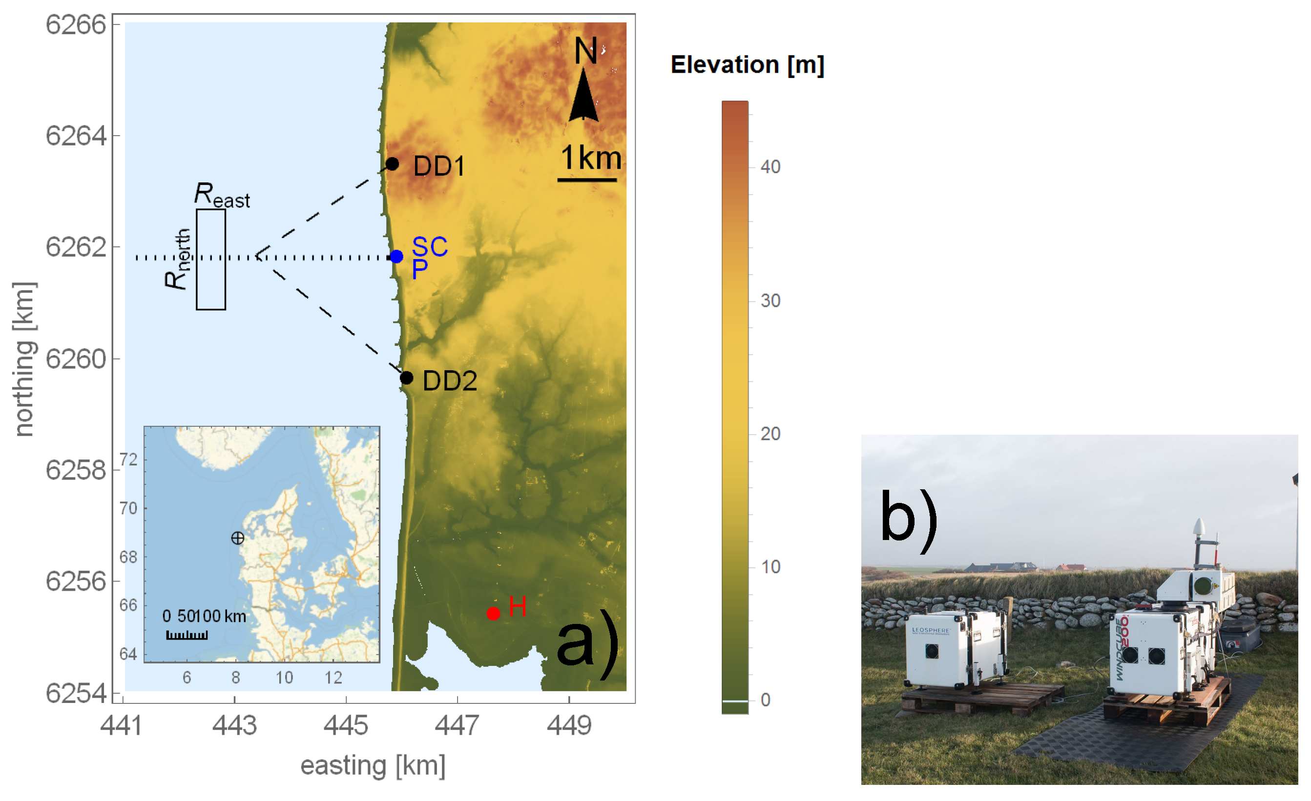
The focus of the RUNE experiment was on coastal winds. Several LiDARs and other instruments were deployed to give detailed spatial and temporal information of the wind conditions. A detailed description of the experiment can be found in Floors and Peña [29]. Figure 1 shows the experimental setup on the Danish West Coast. The map shows the location of the LiDAR devices, meteorological mast and a transect perpendicular to the coast where the wind speed was reconstructed (hereafter, the transect). The topography to the south is flat with some dunes at the beach. The northerly part has a steep escarpment on the coastline and a small beach with regularly spaced wave breakers towards the seaside. The transect starts at the position of two LiDARs (SC and P) where the terrain elevation is 26 m. The transect goes towards the West and LiDAR measurements are taken at several levels (see Figure 2). The land is governed by fields, small hedges, distantly spaced houses and small villages. The sea bed is sandy with a gentle slope interrupted by occasional sand banks.
2.1. Sentinel-1A SAR
Sentinel-1A from the European Space Agency (ESA) carries an active microwave C-band SAR system on board. The satellite circumvents the Earth on a sun synchronous orbit, ascending around 6:40 and descending around 18:10 local time. Scenes in Interferometric Wide swath mode (IW) and in Extra Wide swath mode (EW) in vertical co-polarization (VV) and horizontal co-polarization (HH) are used. The resolution of the raw Sentinel-1A SAR image is up to 5 m [31] but the images are averaged to pixel size before the wind retrieval to reduce artefacts from inherent speckle noise and changes in the local incident angle caused by long period waves. For this study 15 SAR images from Sentinel-1A were collected during the RUNE campaign between December 2015 and February 2016 and processed into wind maps. The images include a small region of on the west coast of Denmark (west of 56.50N, 8.12E, see Figure 1) where scanning LiDAR wind measurements over water were available. Table 2 shows an overview of image parameters for each case. The structure of the GMF CMOD5.N is presented in Equation (1) [5,32].
The normalized radar cross section is a function of the wind speed at 10 m v, the angle between radar look direction and wind direction , and the incidence angle . and are functions including the tuning parameters of the model and in the exponent p is 0.625. For wind speed retrievals Equation (1) is inverted numerically. CMOD5.N is developed for VV polarized images and a polarization correction for HH polarized images is applied [33]. At the Technical University of Denmark (DTU), 10 m SAR wind maps are produced using the SAR Ocean Products System (SAROPS) [34].
Wind Direction Input for SAR Wind Retrieval
SAR wind speed retrievals with GMFs need the wind direction as an input. The retrieval algorithm can be very sensitive towards the wind direction input depending on the angle between the wind velocity vector and the radar look angle. Estimation of wind direction from the SAR image itself is possible [35], but for operational wind speed retrievals, the wind direction inputs are typically obtained from global models [34]. For the investigated period several wind direction measurements are available. Local wind direction measurements are used for the SAR wind retrieval in this study.
2.2. LiDAR Measurements
2.2.1. Scanning LiDARs
Three long range scanning LiDARs (Windcube200 using a wave length of 1543 nm) were deployed on the coast line at position DD1, DD2, and SC in Figure 1. Devices, software, and wind speed reconstruction are described in Vasiljević et al. [24]. The RUNE experiment was designed to study the development of the coastal marine boundary layer and scan patterns were optimized for that purpose. The LiDARs were set up to perform two types of scans; one LiDAR performs sector scans, two LiDARs perform coordinated dual Doppler scans and a detailed description of the measurements is available [29,36]. Averages of 10 min, are used for this study and the LiDAR measurements are treated as point measurements at the reconstruction points. A brief description of the scans used for this study follows:
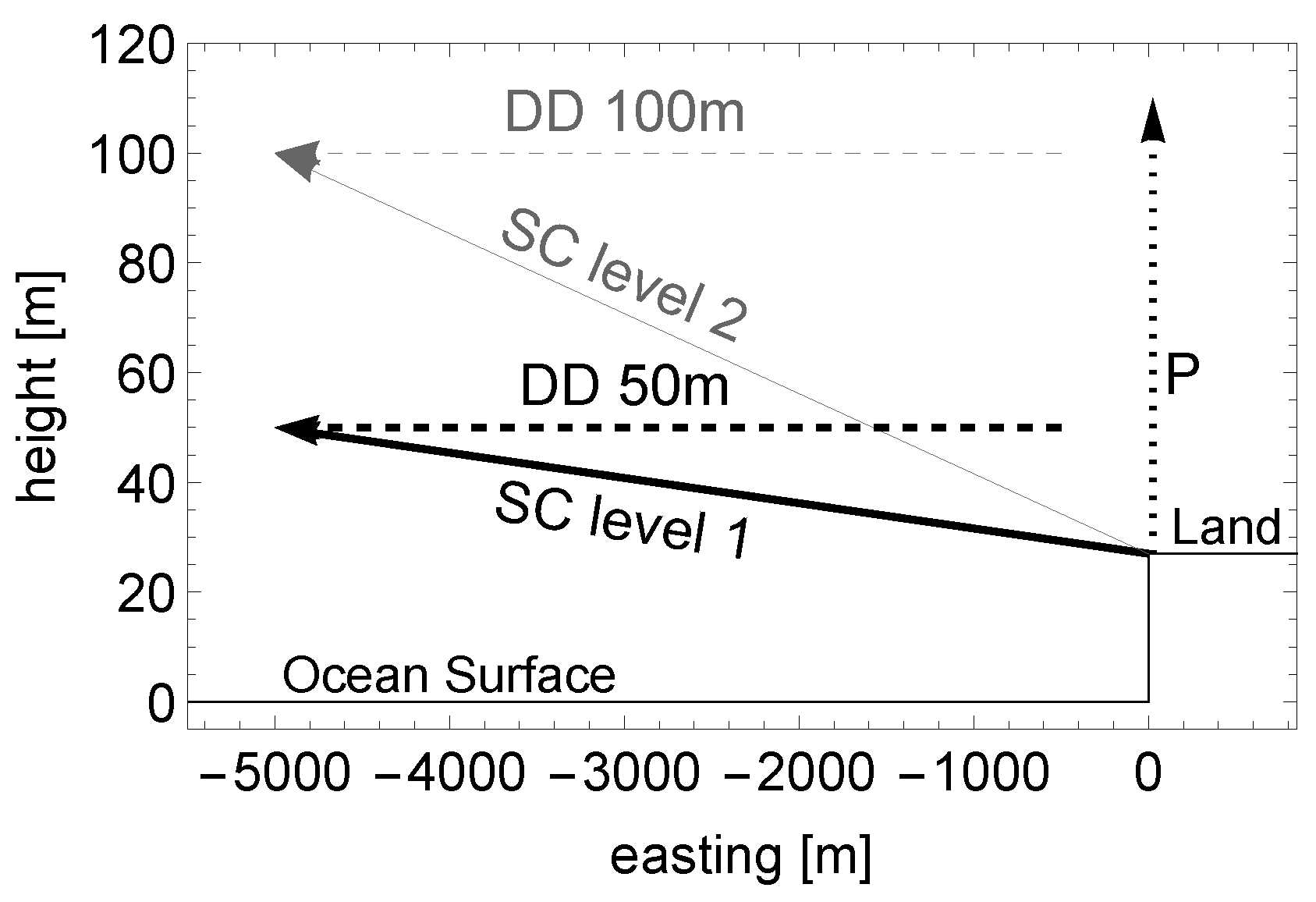
The scanning LiDAR at position SC performs sector scans over a arc at three elevations with three inclinations (see Figure 4 in Floors and Peña [29]). The wind speed is reconstructed at the dotted line in Figure 1. A vertical cut through the transect is shown in Figure 2 with the lowest two inclinations of 0.27 (SC level 1) and 0.54 (SC level 2). The height of SC level 1 used in this study is 26 m at the coast line and increases linearly to 50 m at 5 km offshore. For two cases, the scanner was scanning horizontally at a fixed elevation of 26 m.
Two scanning LiDARs at position DD1 and DD2 performed temporal and spatial coordinated dual Doppler scans at the transect (Figure 1). The horizontal wind speed is reconstructed from two line of sight velocities on the transect at 50 m and 100 m as shown by the dashed lines Figure 2 (A detailed overview can be found in Figure 4 in Floors and Peña [29]).
2.2.2. Profiling LiDAR
A vertically profiling LiDAR (Windcube v2 pulsed LiDAR) was placed at position P on the coastline at 26 m elevation. The performance of this type of profiling LiDAR has been extensively tested against data from meteorological masts, e.g., Peña et al. [20]. The LiDAR measures wind profiles from 40 m to 300 m and 10-min averaged data from this instrument is used for this study. The wind direction input for the SAR wind retrieval is taken from the 10 min mean wind direction at 50 m height.
2.3. Meteorological Mast
DTU has a test center for tall wind turbines at Høvsøre including a 116.5 m tall meteorological mast equipped with cup anemometers, wind vanes, sonic anemometers and temperature measurements [37]. It is located 6 km south of the central scanning LiDAR position SC (position H in Figure 1). The mast provides averaged profiles of wind speed, wind direction, and temperature. An important parameter determining the characteristic of the wind profile is the atmospheric stratification characterized by the Obukov length, see e.g., Wyngaard [38]. The Obukov length L is defined as:
where is the friction velocity, the vertical sensible heat flux, g the gravitational constant and the von Kármán constant. 30-min time series are used to calculate the Obukov length L.
2.4. Available Cases
For the period from December 2015 to February 2016, 32 Sentinel-1A images are available. Of these, four images coincide only with sector scan data, 3 only with dual Doppler data, and 8 with both Dual Doppler and sector scan data. Table 2 shows an overview of the SAR image properties for the 15 cases where SAR and LiDAR observations are collocated and Table 3 shows the meteorological conditions. The conditions tended to be stable with 4 neutral, 2 stable, and 8 very stable cases. No stability class was available for Case 9.
2.5. Method for Comparing SAR and LiDAR Data
The previously described scanning LiDAR measurements are of high accuracy [24] and are used as the reference for the SAR wind retrievals. Comparisons with meteorological mast measurements before the RUNE experiment yielded 0.1% error for the dual Doppler and 0.2% error for the sector scans [39]. Comparisons between the LiDAR scans and the SAR retrievals need to incorporate intrinsic averaging processes in the data acquisition, which depend on the measurement device. Long range scanning LiDARs measure the wind speed in a thin control volume of approximately 100 m length [21] and the backscatter, due to a volume of particles, is received. SAR winds are calculated from the averaged normalized radar cross section of a 500 m grid cell and therefore the resulting wind speed is similar to a 2D spatial average of the wind speeds within this cell. Backscatter from each SAR resolution cells is measured for a few seconds rendering it an instantaneous measurement. Wind speed measurements from SAR and scanning LiDARs generally have a vertical, horizontal and temporal displacement that needs to be addressed.
2.5.1. Vertical Displacement
All LiDAR measurements from the sector scan and dual Doppler are above 10 m. Assuming that these measurements are within the surface boundary layer allows the use of wind profiles in order to extrapolate the measurements to 10 m. Wind profiles in the surface layer are valid for ensemble mean wind speeds [38]. Therefore, 10 min averages of the wind speeds are used.
In lack of a reliable stability measure at the offshore transect, logarithmic wind profiles for neutral stratification are applied. In order to account for the changing roughness of water with the wind speed, the Charnock’s relation is included. Extrapolation from the LiDAR measurement height is performed using the following set of equations:
Here is the mean wind speed at height of the LiDAR measurement, is the mean wind speed at 10 m, is the friction velocity, g the gravitational constant, is the von Kármán constant, and the aerodynamic roughness. The Charnock parameter is often described as a function of wind speed or wave parameters and it is often used in the range between 0.011 and 0.018 [40]. The 50 m dual Doppler level and first level of the sector scan, between 26 m and 50 m, as shown in Figure 2 are extrapolated down to 10 m. Extrapolations to 10 m from this method have uncertainties but it is a standard method applied in lack of accurate stability information offshore for all cases, as e.g., in Chang et al. [10], Hasager et al. [14].
2.5.2. Temporal and Horizontal Displacement
Wind speeds at a point can change quickly over time due to their turbulent nature. Therefore, comparisons between measurement devices should be averaged over the same time period. LiDAR measurements are averaged over 10 min and SAR wind retrievals give an almost instantaneous wind speed. This difference is usually addressed by spatially averaging SAR winds around the in LiDARsitu measurement with a box window [17,41] or more advanced footprint averaging methods [16]. Rectangular averaging bins centered around the LiDAR transect with perpendicular to the coast (East-West) and parallel to the coast (North-South) are applied for this study. Figure 1 shows one rectangular bin of and for the averaging of the SAR wind retrievals as an example. The LiDAR measurements on the transect shown in Figure 2 are also averaged in bins with a length of . This study aims to show the ability of SAR to measure horizontal wind speed gradients correctly. Therefore, it is necessary to keep a high resolution perpendicular to the coast along the transect. is set to 500 m corresponding to one SAR resolution cell, resulting in ten bins over the transect.
Figure 1 shows that the coastline is straight from South to North with a steep escarpment. Therefore, the wind speed is considered homogeneous along the coast line and averaging should not introduce a systematic bias. To test this assumption and to find a compromise between averaging and horizontal displacement between LiDAR and SAR measurements, a sensitivity test of is performed. The difference between the closest SAR resolution cell to the center of each bin , and the bin averaged SAR wind speeds using an area of by are calculated using the following equation,
where is the wind speed in each resolution cell and N the number of resolution cells within each bin. In order to avoid contamination from land, only the SAR image bins from 1.5 km to 5 km distance to shore are used. Table 4 shows how the number of SAR resolution cells used for averaging increases with . The mean and the absolute mean of all values are calculated from Equation (6). is small compared to the retrieved wind speed for all , supporting the assumption of flow homogeneity along this coast. Spatial averaging takes variability in the wind speed into account and makes the SAR winds more comparable to 10-minute mean wind speeds. The absolute mean differences indicate how much fluctuations of the SAR wind are included in each averaging bin. The largest change occurs from 1 to 2 cells. Since it is desired to include these deviations from , choosing between 1 km to 2 km is a good compromise for averaging SAR wind speeds and considering the horizontal displacement between SAR and LiDAR measurement.
Lastly, the RMSE in Table 4 is the RMSE between dual Doppler and SAR compared in each averaging cell. Including one SAR resolution cell corresponding to no averaging gives the largest RMSE. The effect of including more SAR resolution cells is small between 1 km and 3 km. = 1.5 km is used in the remaining part of this study.
3. Results
As a starting point, SAR and LiDAR wind speeds are compared over the transect to determine if SAR winds show a systematically different behaviour over the distance to shore (Figure 3). Averages of the wind speed for each case are presented to show an overall comparison in a scatter plot (Figure 4). Thereafter, the mean wind speed from SAR and LiDAR systems are calculated to determine the coastal gradients measured from both systems (Figure 5 and Figure 6). Lastly, three cases are presented in more detail to illustrate possible challenges when comparing SAR and scanning LiDAR wind speeds (Figure 7).
3.1. Differences over the Transect
Differences in the wind speeds from SAR and scanning LiDARs are shown in Figure 3. SAR wind retrievals closest to the coast at −500 m have considerable deviations, possibly from reflections of hard targets that are not usable for wind speed retrievals. The scanning LiDARs have ranges of less than 5 km for most cases and therefore the number of observations N decreases when going further offshore. For all cases both LiDAR systems give wind speed measurements from 0 m to −3000 m.
For the comparisons with the dual Doppler in Figure 3a, the SAR wind retrieval measured less wind speed than the LiDAR over the entire transect. The mean differences are constant from −1000 m to −3000 m and increase afterwards with decreasing sample sizes. The standard deviation in each bin is almost constant between −1000 m and −3000 m. Mean differences in the bins between SAR and LiDAR are small over the entire transect for sector scan and SAR comparisons in Figure 3b. The spread in the differences has a tendency to be increasing with the distance from the coast. Possible explanations are the decreasing sample size and the change in the measurements height of the sector scan. Ten out of these 12 cases are measured with a slight inclination of the LiDAR (see Figure 2). Measurements at −1000 m are at 30 m elevation while the measurement height increases with the distance to the coast line to 50 m at −5000 m. Increasing extrapolation height compared to 10 m increases associated uncertainties and is assumed to explain part of the increasing spread with the distance to the coast. Mean bias and standard deviation from Figure 3 indicate that SAR and LiDAR give meaningful comparisons from −1000 m and further offshore.
Table 5 summarizes biases and standard deviations over all bins. For both systems there is a bias towards lower wind speed in the SAR wind retrieval. The bias compared to the dual Doppler over all bins is −0.57 . The sector scan comparisons have a lower overall bias of −0.17 with almost no bias until −3000 m.
3.2. Spatially Averaged Wind Speed
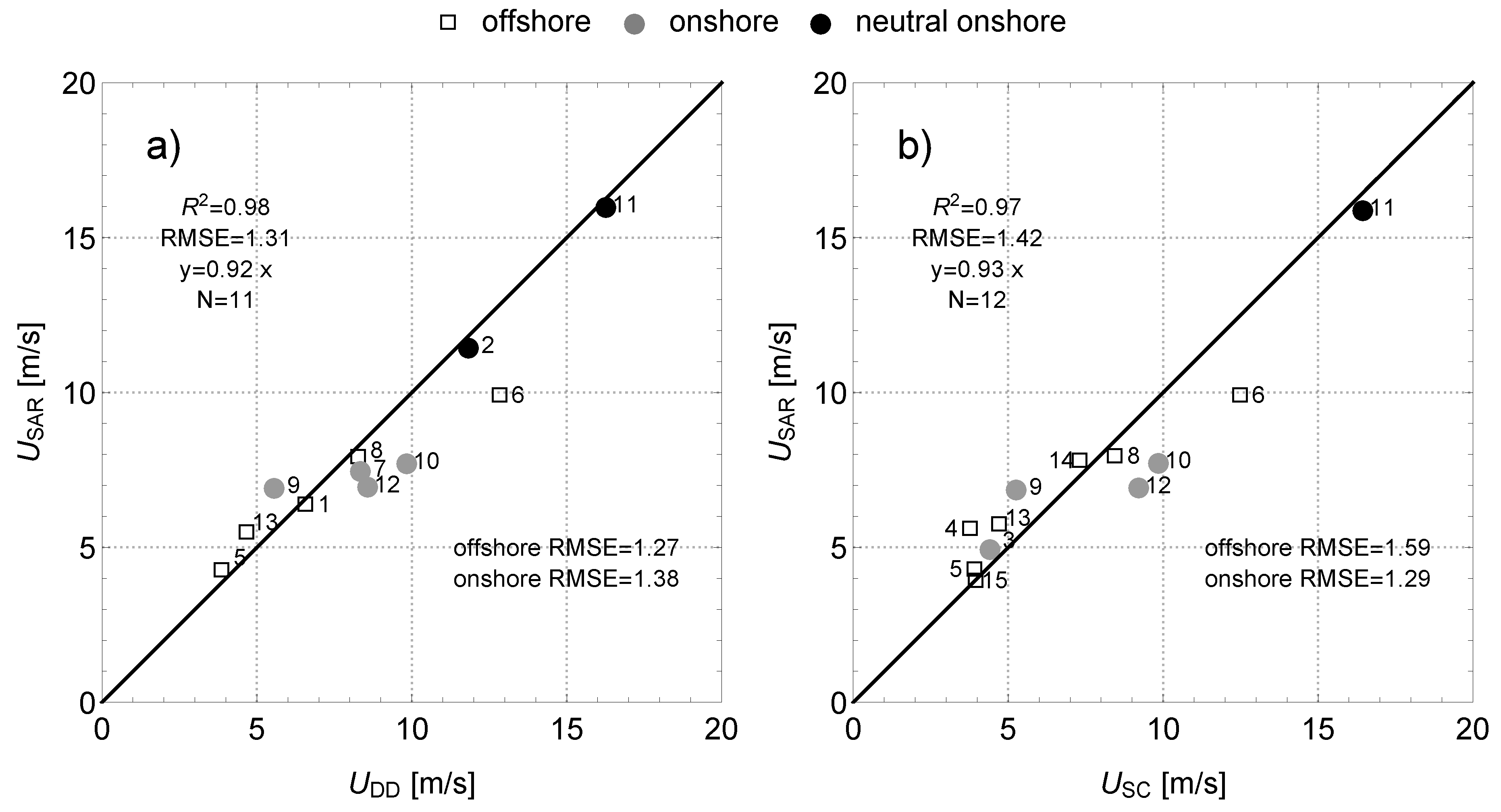
The average of SAR and scanning LiDARs wind speeds is taken respectively for each case from −1000 m until the maximum range available. This results in a single averaged wind speed over the transect for SAR and LiDAR measurements. Figure 4 shows the resulting scatter plots using the dual Doppler and the sector scan. The RMSE is 1.31 for the dual Doppler and 1.42 for the sector scan. The averaged wind speeds are between 4 and 10 for most cases and only one case has wind speeds as high as 16 . Data from Table 3 are used to classify the cases by wind direction and atmospheric stability. Case 2 and 11 have neutral conditions at the mast location with onshore winds and are indicated with black markers. For those cases the assumption of neutral stratification and horizontal homogeneity used for the extrapolation of LiDAR wind measurements are best met and wind speeds from SAR and LiDAR agree within 0.5 . RMSEs for onshore and offshore cases range between 1.27 and 1.58 (see Figure 4). Case 6 has a neutral stability class and shows large deviation, heavily affecting the offshore RMSEs.
3.3. Ensemble Averaged Wind Speed
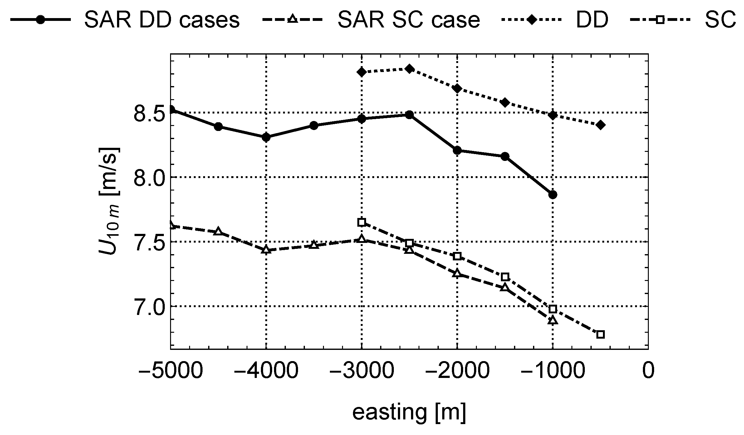
Transects of the mean wind speed from SAR and LiDAR calculated for all cases are shown in Figure 5. In order to exclude the influence of sample size within each bin, LiDAR measurements are only plotted until −3000 m where all LiDAR systems are available for all cases (see Figure 3). The difference between the two SAR wind transects (SAR DD cases and SAR CS cases) is caused by averaging over a different subset of cases from Table 3. Horizontal mean wind speed gradients are present in the scanning LiDAR data and SAR wind, generally with increasing wind speeds when moving further offshore. The absolute magnitude between dual Doppler and SAR DD cases has an offset as expected from the bias in Figure 3. Sector scans and the respective SAR SC cases agree within 0.2 .
In order to get a qualitative estimate of how SAR and LiDARs are measuring the horizontal wind speed gradient, the wind speeds in Figure 5 are nondimensionalized. Wind speeds in each bin from SAR and LiDAR measurements in Figure 5 are divided by their respective wind speed at −3000 m. The nondimensional dual Doppler wind speed in Figure 6a shows a lower gradient than the SAR wind. The nondimensional wind speed in Figure 6b is very close for sector scan and SAR winds, and both systems similarly estimate a relative reduction of the wind speed when approaching the coast.
3.4. Example Cases
Three cases are selected as examples of how SAR and scanning LiDARs measure horizontal wind speed gradients in Figure 7. These examples illustrate some of the issues with extrapolating LiDAR wind measurements down to 10 m. Additional to the lowest level used in Figure 3 to Figure 6, extrapolations from the 100m dual Doppler and the second sector scan level are used, see Figure 2. Cases are chosen according to wind direction and stratification. Case 10 and 11 have onshore winds with neutral and stable stratification at the mast location respectively. For case 6 the wind direction is offshore and the stratification is neutral. This case also has a large influence on the overall RMSE. Their position in the scatter plot is shown in Figure 4.
Case 11 has onshore winds with a direction of 250 and neutral stratification at the mast location. Figure 4 shows that SAR and both LiDAR system agree well when averaged. Figure 7 shows that extrapolated 10 m mean wind speeds agree between all systems and scanning levels. Wind speeds from SAR give lower wind speeds but mostly agree within 1 . Especially, both sector scan levels and the 50 m dual Doppler level are in good agreement with the SAR wind speeds. This suggests that the assumptions of a logarithmic wind profile are indeed valid for this case. Coastal wind speed gradients are similar and present for all systems.
Case 10 in Figure 7 has a wind direction of 264 which is similar to case 11 but the stratification is stable at the mast location (see Table 3). SAR winds and the LiDARs disagree with differences up to 3 . Moreover, both sector scan levels indicate a strong horizontal wind speed gradient, while the dual Doppler measurements suggest a much lower gradient. Extrapolations from 50 m and 100 m disagree with an offset around 1 . Stable stratification can explain both of these behaviours. Applying a neutral wind profile in stable conditions to extrapolate down to 10 m overestimates this wind speed. This overestimation increases with a growing extrapolation height. The sector scan at the lowest elevation at −1000 m with approximately 30 m has the lowest difference of 1 compared to the SAR (for elevation of the scans, see Figure 2). Application of a stability correction with a reliable stability estimation would likely improve the results. Case 12 has a very similar behaviour (not shown here).
Case 6 in Figure 7 has offshore wind directions of 149 . Extrapolation to 10 m for all LiDAR systems with measurement heights between 30 m and 100 m agree within 1 after extrapolation to 10 m. The disagreement between SAR and the LiDARs ranges between 2 and 3.5 . SAR winds and LiDARs are showing a similar horizontal gradient with a reduction of approximately 1.5 from −5000 m compared to −1000 m. The assumption of neutral stratification for the application of a logarithmic wind profile is assumed valid in this case but the assumption of horizontal terrain homogeneity is violated due to the change of surface roughness between land and sea. An equilibrium layer grows with approximately 1/200 from the place of the roughness change under neutral conditions [42,43] but the height of an internal boundary layer can grow much faster in the order of 1/10 [44]. With the coastline in Figure 1 following a South-North direction the internal boundary layer should have already grown to the measurement height of the LiDARs for the points further offshore. Internal boundary layers are unlikely to cause large errors for the LiDAR extrapolation in this case.
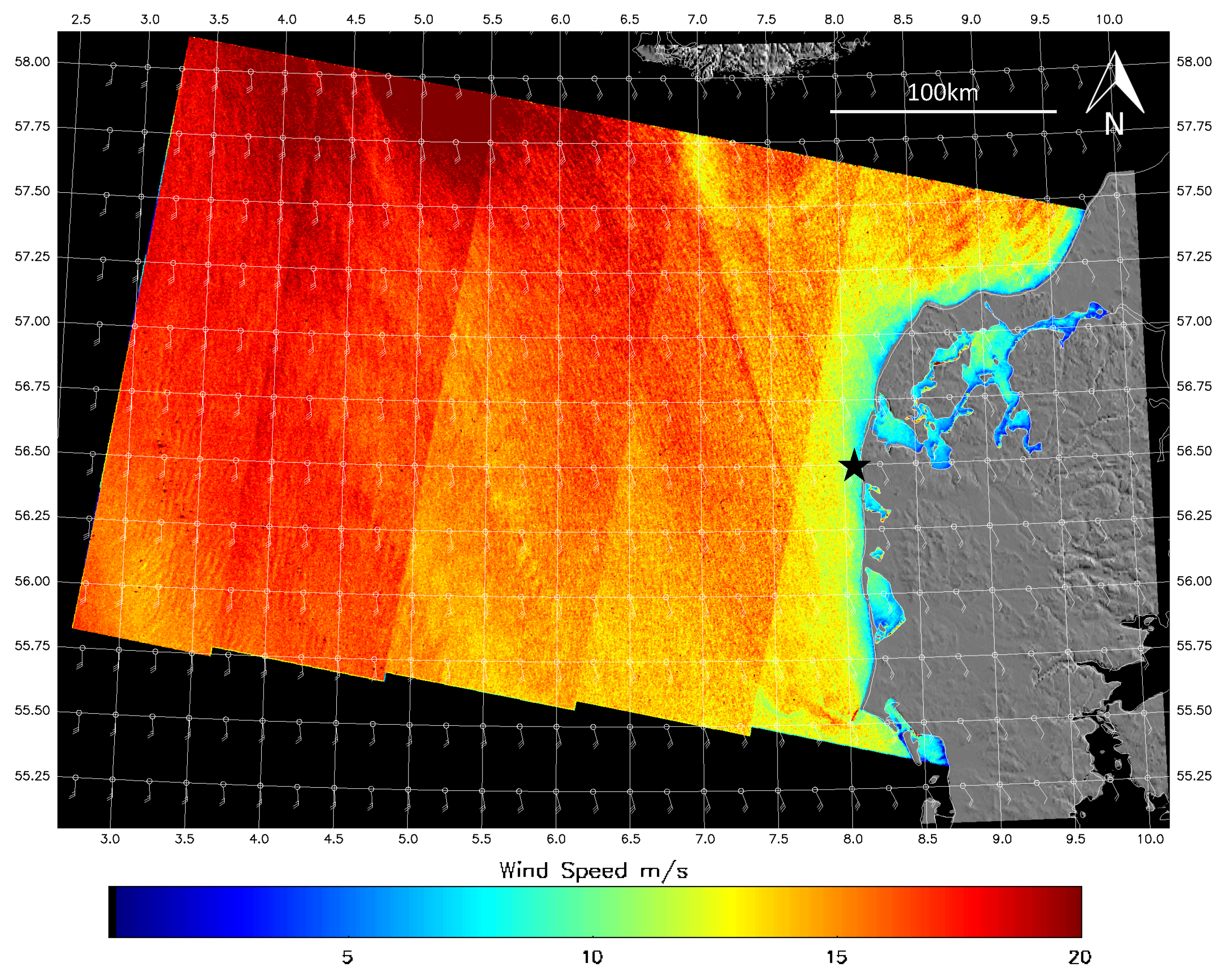
The SAR image of case 6 is taken at an incidence angle of 27. The entire transect lies within the first subswath of Sentinel-1A’s EW mode as shown in Figure 8. This SAR wind map has clear discontinuities in range direction between subswaths, most notably between the first and the second subswath going from East to West. These discontinuities in the wind speed are likely due to insufficient calibration. Other SAR images in this study do not suffer from these pronounced discontinuities. Adding a constant of 0.033 to the normalised radar cross section in the first subswath would remove the discontinuity to the second subswath. This very simple way of adjusting the backscatter results in approximately 2.2 higher wind speed retrieval on the transect and removes most of the offset in case 6 as shown in Figure 7. Using this SAR wind speed would reduce the RMSE in Figure 4.
4. Discussion
This study shows the results of 15 SAR Sentinel-1A scenes processed to maps of equivalent neutral wind speed and compares them to scanning LiDAR wind measurements. Comparison of SAR and LiDAR measurements is challenging because of intrinsic differences between the measurement techniques. Horizontal and temporal displacement of SAR and LiDAR measurements have been taken into account, finding a compromise between local homogeneity of the flow and the need for additional spatial averaging. Spatial averages over the transect for each case from LiDAR wind measurements and SAR wind retrievals yield an RMSE of 1.31 for the dual Doppler set up and 1.42 for the sector scans, which is in the range of studies using measurements from meteorological mast with larger sample sizes in Table 1. Wind directions from land or from sea seem to have little influence on the RMSE of the comparisons, similar to e.g., [10]. The wind direction over the entire SAR image deviates locally from the assumed constant 10-min average used for the retrieval. Local measurements of the wind direction have shown to have lower RMSEs compared to other methods [11,15]. Comparisons of the input wind direction with the scanning LiDAR wind directions yield up to 10 difference.
Unlike previous validation studies in coastal areas [9,10,11,12,13,14,15,16], the use of scanning LiDARs made comparisons to SAR wind speeds on a transect possible. The effect of currents, waves and limited fetch on e.g., the Charnock parameter in coastal waters has not been taken into account in this study. Results in Figure 3a show that the mean difference and standard deviation within each bin are similar as long as the number of available samples is constant. Between −3000 m and −5000 m the decreasing sample size influences the results. Figure 3b shows that the standard deviation within each bin decreases when approaching the coast. This is likely caused by a decreased extrapolation uncertainty associated with lower measurement heights of the sector scans shown in Figure 2. SAR wind retrievals with CMOD5.N are in good agreement with scanning LiDAR wind measurements as close as 1 km to the coast.
Coastal gradients are visible, both in SAR wind speeds and scanning LiDAR measurements. The absolute value of the ensemble averaged wind speed can deviate between SAR and scanning LiDARs, see Figure 5. One reason for the bias is likely a calibration issue as seen from case 6 in Figure 7, where removing the discontinuity from the first to the second subswath rectifies the bias in wind speed. Nondimensionalizing the transects reveals that the relative reduction in wind speed is similar between SAR and LiDAR, see Figure 5 and Figure 6. The relative mean wind reduction from 3 km to 1 km offshore is 7% and 4% for SAR and dual Doppler respectively. Some of this difference can be accounted to differences in the measurement height of SAR (on the ocean surface) and the dual Doppler (at 50 m). Horizontal mean wind speed gradients become less pronounced with the measurement height for this location and time period, see Figure 15 in Floors et al. [36]. A reduction of the mean wind speed by 8% from 3 km to 1 km offshore is observed for SAR and sector scans with very good agreement.
This site in Northwestern Denmark has a simple topography, but a steep escarpment makes it representative for many coastal areas with such features and simple coastal geometry. The period over the winter of 2015/2016 was particular windy at this location [29] and the stratification of the atmosphere was either neutral or stable for the presented cases. For 12 of the 15 cases wind speeds at 10m height range between 4 and 10 and no case exceeding 16 is present in the data. Therefore, results are representative for these atmospheric conditions.
A portion of the difference between SAR and LiDAR wind speeds can likely be accounted by the vertical extrapolation. Using logarithmic wind profiles causes erroneous extrapolations of wind speeds at 10 m, as shown in the example case 10 in Figure 7. This is supported by two cases where assumptions from the logarithmic wind profile are fulfilled; there SAR wind retrieval and LiDAR measurements agree within 0.5 , see Figure 4. The atmospheric stratification was either neutral or stable for the cases examined here while CMOD5.N and the logarithmic extrapolation assume neutral conditions. The error from extrapolation in this study will not systematically improve the results, since it introduces a bias compared to in situ measurements [45,46]. The estimated RMSE should therefore be seen as a conservative estimate for the presented cases.
The energy density of the wind scales approximately with the cubed mean wind speed, making the energy yield of wind turbines very sensitive to the wind speed. Therefore, the quantification of pronounced horizontal wind speed gradients in the coastal zone is extremely important for the placement of offshore wind farms. The value of SAR derived wind resource maps largely depends on the validity close to shore according to Hasager et al. [9] and Hasager et al. [14]. This validation study further supports the use of SAR wind retrievals for wind resource mapping in coastal waters.
5. Conclusions
Sentinel-1A SAR wind retrievals with CMOD5.N from the coastline up to 5 km offshore have been compared to scanning LiDAR wind measurements in the Northern Sea on the Danish West Coast, for the first time showing how LiDAR and SAR measure typical wind speed reduction when approaching the coast from offshore. Differences between spatially averaged wind speeds are comparable to validations with point measurements found in previous studies. Results indicate that C-band SAR wind retrievals are accurate as close as 1 km from the coastline where reflections start to affect the scattering from the ocean surface. Changes in the wind speed over the distance from shore are detected by both SAR wind retrievals and LiDAR. The relative reduction between 3 km and 1 km offshore in the wind speed is 7% to 8% from SAR and 4% to 8% for the LiDARs. These results support the use of SAR to identify coastal wind speed gradients, which are important for many applications such as offshore wind energy planning, ship traffic, and harbour management.
Scanning LiDAR technology will be used further in the future to study the transition of atmospheric boundary layers at the coastline. This could lead to further validation studies of coastal SAR wind retrievals for more sites, and different coastal geometries.
Acknowledgments
We would like to acknowledge the funding from the ForskEL program to the project ‘RUNE’ (Nr. 12263), Johns Hopkins University Applied Physics Laboratory and the National Atmospheric and Oceanographic Administration (NOAA) for the use of the SAROPS system, and ESA for providing public access to data from Sentinel-1A. A personal thanks to Charlotte Hasager, Jens Nørkær Sørensen and Sung Yong Kim for their comments on the manuscript.
Author Contributions
Tobias Ahsbahs has decided on the direction of the study with help from Merete Badger, implemented the code for comparison, and done the writing and implementation of the co-author’s comments. Merete Badger has supervised the project work and maintains the SAROPS systems used for wind retrievals. Ioanna Karagali supported the method and interpretation of the results with comments and discussions. Xiaoli Larsén has provided guidance on the meteorological side of the method. All co-authors have participated in revising the draft from the first collection of ideas to the final version of the paper.
Conflicts of Interest
The authors declare no conflict of interest.
Abbreviations
The following abbreviations are used in this manuscript:
| SAR | Synthetic Aperture Radar |
| LiDAR | Light Detection and Ranging |
| GMF | Geophysical Model Function |
| CMOD | C-band model |
| CMOD5.N | C-band model 5.N |
| RMSE | Root Mean Square Error |
| RUNE | Reducing uncertainty of near-shore wind resource estimates using onshore LiDAR |
| SAROPS | SAR Ocean Products System |
| DD | Dual Doppler |
| SC | Sector Scan |
| STD | Standard deviation |
| DTU | Technical University of Denmark |
References
- Dagestad, K.F.; Horstmann, J.; Mouche, A.; Perrie, W.; Shen, H. Wind Retrieval From Synthetic Aperture Radar—An Overview; SeaSar 2012 Oceanography Workshop: Tromsø, Norway, 2013. [Google Scholar]
- Karagali, I.; Larsen, X.G.; Badger, M.; Peña, A.; Hasager, C.B. Spectral Properties of ENVISAT ASAR and QuikSCAT Surface Winds in the North Sea. Remote Sens. 2013, 5, 6096–6115. [Google Scholar] [CrossRef]
- Stoffelen, A.; Anderson, D. Scatterometer data interpretation: Estimation and validation of the transfer function CMOD4. J. Geophys. Res. 1997, 102, 5767. [Google Scholar] [CrossRef]
- Quilfen, Y.; Chapron, B.; Elfouhaily, T.; Katsaros, K.; Tournadre, J. Observation of tropical cyclones by high-resolution scatterometry. J. Geophys. Res. 1998, 103, 7767. [Google Scholar] [CrossRef]
- Hersbach, H. Comparison of C-Band Scatterometer CMOD5.N Equivalent Neutral Winds with ECMWF. J. Atmos. Ocean. Technol. 2010, 27, 721–736. [Google Scholar] [CrossRef]
- Gade, M.; Alpers, W. Using ERS-2 SAR images for routine observation of marine pollution in European coastal waters. Sci. Total Environ. 1997, 237–238, 441–448. [Google Scholar]
- Romeiser, R.; Alpers, W. An improved composite surface model for the radar backscattering cross section of the ocean surface: 2. Model response to surface roughness variations and the radar imaging of underwater bottom topography. J. Geophys. Res. Oceans 1997, 102, 25251–25267. [Google Scholar] [CrossRef]
- Christiansen, M.B.; Hasager, C.B.; Thompson, D.R.; Monaldo, F.M. Ocean winds from synthetic aperture radar. In Ocean Remote Sensing: Recent Techiniques and Applications; Chapter Ocean Wind; Research Signpost: Kerala, India, 2008; pp. 31–54. [Google Scholar]
- Hasager, C.B.; Mouche, A.; Badger, M.; Bingöl, F.; Karagali, I.; Driesenaar, T.; Stoffelen, A.; Peña, A.; Longépé, N. Offshore wind climatology based on synergetic use of Envisat ASAR, ASCAT and QuikSCAT. Remote Sens. Environ. 2015, 156, 247–263. [Google Scholar] [CrossRef]
- Chang, R.; Zhu, R.; Badger, M.; Hasager, C.B.; Xing, X.; Jiang, Y. Offshore wind resources assessment from multiple satellite data and WRF modeling over South China Sea. Remote Sens. 2015, 7, 467–487. [Google Scholar] [CrossRef]
- Takeyama, Y.; Ohsawa, T.; Kozai, K.; Hasager, C.B.; Badger, M. Effectiveness of WRF wind direction for retrieving coastal sea surface wind from synthetic aperture radar. Wind Energy 2014, 16, 865–878. [Google Scholar] [CrossRef]
- Chang, R.; Zhu, R.; Badger, M.; Hasager, C.B.; Zhou, R.; Ye, D.; Zhang, X. Applicability of synthetic aperture radar wind retrievals on offshore wind resources assessment in Hangzhou Bay, China. Energies 2014, 7, 3339–3354. [Google Scholar] [CrossRef]
- Takeyama, Y.; Ohsawa, T.; Kozai, K.; Hasager, C.B.; Badger, M. Comparison of geophysical model functions for SAR wind speed retrieval in japanese coastal waters. Remote Sens. 2013, 5, 1956–1973. [Google Scholar] [CrossRef]
- Hasager, C.B.; Badger, M.; Peña, A.; Larsén, X.G.; Bingöl, F. SAR-based wind resource statistics in the Baltic Sea. Remote Sens. 2011, 3, 117–144. [Google Scholar] [CrossRef]
- Christiansen, M.B.; Koch, W.; Horstmann, J.; Hasager, C.B.; Nielsen, M. Wind resource assessment from C-band SAR. Remote Sens. Environ. 2006, 105, 68–81. [Google Scholar] [CrossRef]
- Hasager, C.B.; Dellwik, E.; Nielsen, M.; Furevik, B.R. Validation of ERS-2 SAR offshore wind-speed maps in the North Sea. Int. J. Remote Sens. 2004, 25, 3817–3841. [Google Scholar] [CrossRef]
- Monaldo, F.M.; Thompson, D.R.; Beal, R.C.; Pichel, W.G.; Clemente-Colón, P. Comparison of SAR-derived wind speed with model predictions and ocean buoy measurements. IEEE Trans. Geosci. Remote Sens. 2001, 39, 2587–2600. [Google Scholar] [CrossRef]
- Monaldo, F.M.; Thompson, D.R.; Pichel, W.G.; Clemente-Colon, P. A systematic comparison of QuikSCAT and SAR ocean surface wind speeds. IEEE Trans. Geosci. Remote Sens. 2004, 42, 283–291. [Google Scholar] [CrossRef]
- Monaldo, F.; Jackson, C.; Li, X.; Member, S.; Pichel, W.G. Preliminary Evaluation of Sentinel-1A Wind Speed Retrievals. IEEE J. Sel. Top. Appl. Earth Obs. Remote Sens. 2015, 8, 2638–2642. [Google Scholar] [CrossRef]
- Peña, A.; Hasager, C.B.; Gryning, S.E.; Courtney, M.; Antoniou, I.; Mikkelsen, T. Offshore wind profiling using light detection and ranging measurements. Wind Energy 2009, 12, 105–124. [Google Scholar] [CrossRef]
- Vasiljević, N. A Time-Space Synchronization of Coherent Doppler Scanning LiDARs for 3D Measurements of Wind Fields. Ph.D. Thesis, Technical University of Denmark, Lyngby, Denmark, 2014. [Google Scholar]
- Gottschall, J.; Courtney, M.; Wagner, R.; Jørgensen, H.; Antoniou, I. LiDAR profilers in the context of wind energy—A verification procedure for traceable measurements. Wind Energy 2012, 15, 147–159. [Google Scholar] [CrossRef]
- Courtney, M. Calibrating Nacelle LiDARs; DTU Wind Energy: Roskilde, Denmark, 2013; p. 43. [Google Scholar]
- Vasiljević, N.; Lea, G.; Courtney, M.; Cariou, J.p.; Mann, J. Long-Range WindScanner System. Remote Sens. 2016, 8, 1–24. [Google Scholar] [CrossRef]
- Berg, J.; Vasiljevíc, N.; Kelly, M.; Lea, G.; Courtney, M. Addressing Spatial Variability of Surface-Layer Wind with Long-Range WindScanners. J. Atmos. Ocean. Technol. 2014, 32, 518–527. [Google Scholar] [CrossRef]
- Barthelmie, R.; Badger, J.; Pryor, S.; Hasager, C.B.; Christiansen, M.; Jørgensen, B. Offshore Coastal Wind Speed Gradients: Issues for the design and development of large offshore windfarms. Wind Eng. 2007, 31, 369–382. [Google Scholar] [CrossRef]
- Doubrawa, P.; Barthelmie, R.J.; Pryor, S.C.; Hasager, C.B.; Badger, M. Satellite winds as a tool for offshore wind resource assessment: The Great Lakes Wind Atlas. Remote Sens. Environ. 2015, 168, 349–359. [Google Scholar] [CrossRef]
- Karagali, I.; Badger, M.; Hahmann, A.N.; Peña, A.; Hasager, C.B.; Sempreviva, A.M. Spatial and temporal variability of winds in the Northern European Seas. Renew. Energy 2013, 57, 200–210. [Google Scholar] [CrossRef]
- Floors, R.; Peña, A. The RUNE experiment—A database of remote-sensing observations of near-shore winds. Remote Sens. 2016, 8, 1–15. [Google Scholar] [CrossRef]
- Jacobsen, S.; Lehner, S.; Hieronimus, J.; Schneemann, J.; Kühn, M. Joint Offshore Wind Field Monitoring With Spaceborne Sar and Platform-Based Doppler LiDAR Measurements. In Proceedings of the 36th International Symposium on Remote Sensing of Environment, Berlin, Germany, 1–15 May 2015; Volume XL-7/W3. [Google Scholar]
- De Zan, F.; Guarnieri, A.M. TOPSAR: Terrain observation by progressive scans. IEEE Trans. Geosci. Remote Sens. 2006, 44, 2352–2360. [Google Scholar] [CrossRef]
- Hersbach, H.; Stoffelen, A.; De Haan, S. The Improved C-Band Geophysical Model Function CMOD5; European Space Agency (Special Publication): Paris, France, 2005; Volume 112, pp. 863–870. [Google Scholar]
- Mouche, A.A.; Hauser, D.; Daloze, J.F.; Guérin, C. Dual-polarization measurements at C-band over the ocean: Results from airborne radar observations and comparison with ENVISAT ASAR data. IEEE Trans. Geosci. Remote Sens. 2005, 43, 753–769. [Google Scholar] [CrossRef]
- Monaldo, F.M.; Jackson, C.; Pichel, W.; Li, X. A Weather Eye on Coastal Winds. Eos 2015, 96, 1–8. [Google Scholar] [CrossRef]
- Koch, W. Directional analysis of SAR images aiming at wind direction. IEEE Trans. Geosci. Remote Sens. 2004, 42, 702–710. [Google Scholar] [CrossRef]
- Floors, R.; Lea, G.; Peña, A.; Karagali, I.; Ahsbahs, T. Report on RUNE ’s Coastal Experiment and First Inter-Comparisons between Measurements Systems; E-Report DTU Wind Energy: Roskilde, Denmark, 2016. [Google Scholar]
- Peña, A.; Floors, R.; Sathe, A.; Gryning, S.E.; Wagner, R.; Courtney, M.S.; Larsen, X.G.; Hahmann, A.N.; Hasager, C.B. Ten Years of Boundary-Layer and Wind-Power Meteorology at Hovsore, Denmark. Bound. Layer Meteorol. 2016, 158, 1–26. [Google Scholar] [CrossRef]
- Wyngaard, J.C. Turbulence in the Atmosphere; Cambridge University Press: Cambridge, UK, 2010; p. 392. [Google Scholar]
- Simon, E.; Courtney, M. A Comparison of Sector-Scan and Dual Doppler Wind Measurements at Høvsøre Test Station—One LiDAR or Two? Technical Report; DTU Wind Energy: Roskilde, Denmark, 2016. [Google Scholar]
- Grachev, A.A.; Fairall, C.W. Dependence of the Monin-Obukhov Stability Parameter on the Bulk Richardson Number over the Ocean. J. Appl. Meteorol. 1996, 36, 406–414. [Google Scholar] [CrossRef]
- Hasager, C.B.; Badger, M.; Nawri, N.; Furevik, B.R.; Petersen, G.N.; Björnsson, H.; Clausen, N.E. Mapping offshore winds around Iceland using satellite synthetic aperture radar and mesoscale model simulations. IEEE J. Sel. Top. Appl. Earth Obs. Remote Sens. 2015, 8, 5541–5552. [Google Scholar] [CrossRef]
- Bradley, E.F. A micrometeorological study of velocity profiles and surface drag in the region modified by a change in surface roughness. Q. J. R. Meteorol. Soc. 1968, 94, 361–379. [Google Scholar] [CrossRef]
- Rao, K.; Wyngaard, J.C.; Cote, O. The Structure of the Two-Dimensional Internal Boundary Layer over a Sudden Change of Surface Roughness. J. Atmos. Sci. 1974, 31, 738–746. [Google Scholar] [CrossRef]
- Troen, I.; Petersen, E.L. European Wind Atlas; Risø National Laboratory: Roskilde, Denmark, 1989; p. 656.
- Kara, A.B.; Wallcraft, A.J.; Bourassa, M.A. Air-sea stability effects on the 10 m winds over the global ocean: Evaluations of air-sea flux algorithms. J. Geophys. Res. Oceans 2008, 113, 1–14. [Google Scholar] [CrossRef]
- Karagali, I.; Peña, A.; Badger, M.; Hasager, C.B. Wind characteristics in the North and Baltic Seas from the QuikSCAT satellite. Wind Energy 2014, 17, 123–140. [Google Scholar] [CrossRef]
Figure 1.
(a) Position of the RUNE experiment at approximately N, E in the Norther Sea on the West Coast of Denmark. Coordinates of the map are in UTM32 WGS84. The transect for the reconstructed LiDAR wind speeds is shown as a dotted line. Positions of the measurement devices are: H: Tall meteorological mast at Høvsøre, DD1 and DD2: scanning LiDARs performing dual Doppler scans (example of coordinated measurements on the transect in dashed lines), SC: scanning LiDAR performing sector scans and profiling LiDAR P. (b) Picture of the deployed scanning LiDAR (SC) and profiling LiDAR (P) for the RUNE experiment. Photo by Mike Courtney.

Figure 2.
Sketch of the scan patterns of the transect in Figure 1 with the ocean on the left and the escarpment on the right. Indicated in black is the lowest sector scan (SC) and in dashed black the lowest elevation of the dual Doppler (DD) at 50 m above the sea. In gray the second elevation of SC and DD (only used for example cases in Section 3.4). Horizontal scans as in cases 14 and 15 are not shown.

Figure 3.
Difference between SAR wind and scanning LiDAR wind measurements at 10 m. The distances on the transect are given in easting from the LiDAR system SC in Figure 1 located on the coast. 0 m is on the coast line and with decreasing easting, points are located further offshore. Individual cases are plotted in gray: (a) 11 cases with the dual Doppler and (b) 12 cases with sector scans. The thick black line is the mean over all cases with error bars indicating one standard deviation within each bin. The top plots show the number of available LiDAR measurements at each distance.
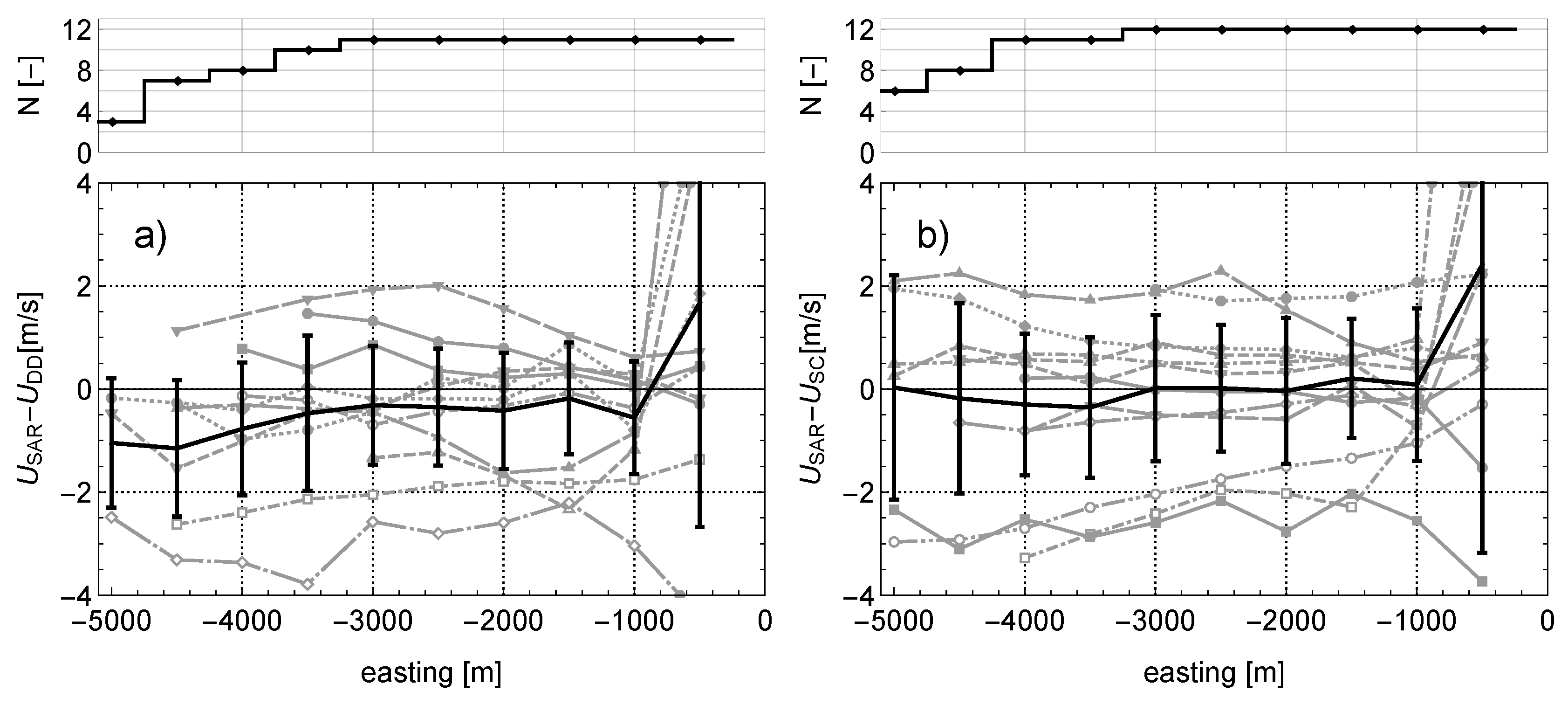
Figure 4.
Scatter plot for the average wind speed on the transect for SAR wind retrieved with CMOD5.N for (a) dual Doppler and (b) sector scan. Plot markers indicate the wind direction at the profiling LiDAR P, onshore for winds from the sea in the west between 180 and 360 and offshore for wind from the land between 0 and 180 . Numbers indicate the case numbers in Table 2 and Table 3.

Figure 5.
Mean 10 m wind speed for all cases from dual Doppler and sector scans and the mean of the collocated SAR wind speeds.
Figure 5.
Mean 10 m wind speed for all cases from dual Doppler and sector scans and the mean of the collocated SAR wind speeds.

Figure 6.
Relative wind speed nodimensionalized with the wind speed at −3000 m for from the LiDAR and the SAR for (a) the dual Doppler and (b) the sector scans.
Figure 6.
Relative wind speed nodimensionalized with the wind speed at −3000 m for from the LiDAR and the SAR for (a) the dual Doppler and (b) the sector scans.
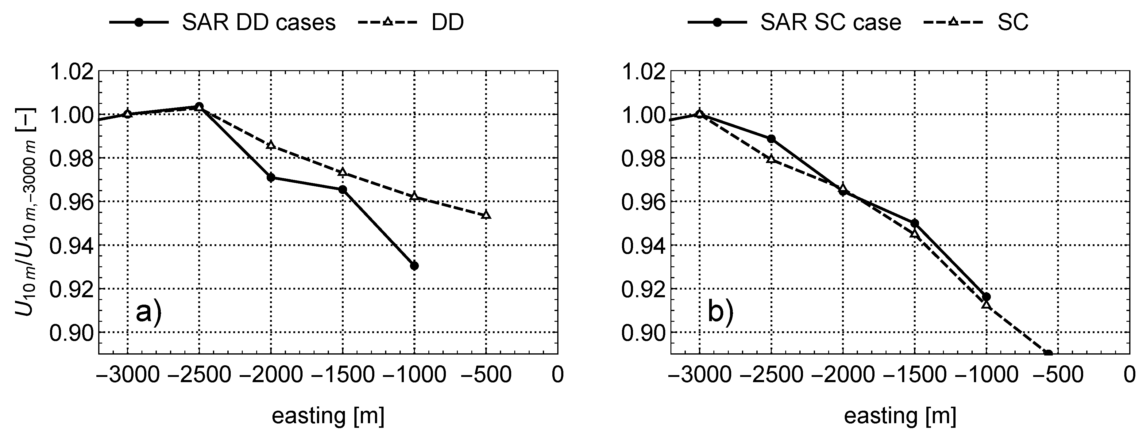
Figure 7.
Wind speeds extrapolated to 10 m from the dual Doppler (DD) and sector scan (SC) and SAR wind speeds. Additionally, to the extrapolation from the lowest level, as used for Figure 3 to Figure 6, extrapolations from the 100 m level for the dual Doppler and the second lowest level of the sector scans are included (see Figure 2). Cases 6, 10 and 11 from Table 2 and Table 3 are shown. SAR winds are in thick black and scanning LiDAR measurements in thin gray. For case 6, the thick gray line shows the SAR wind retrieval with an adjusted normalised radar cross section, in order to remove discontinuities from Figure 8.
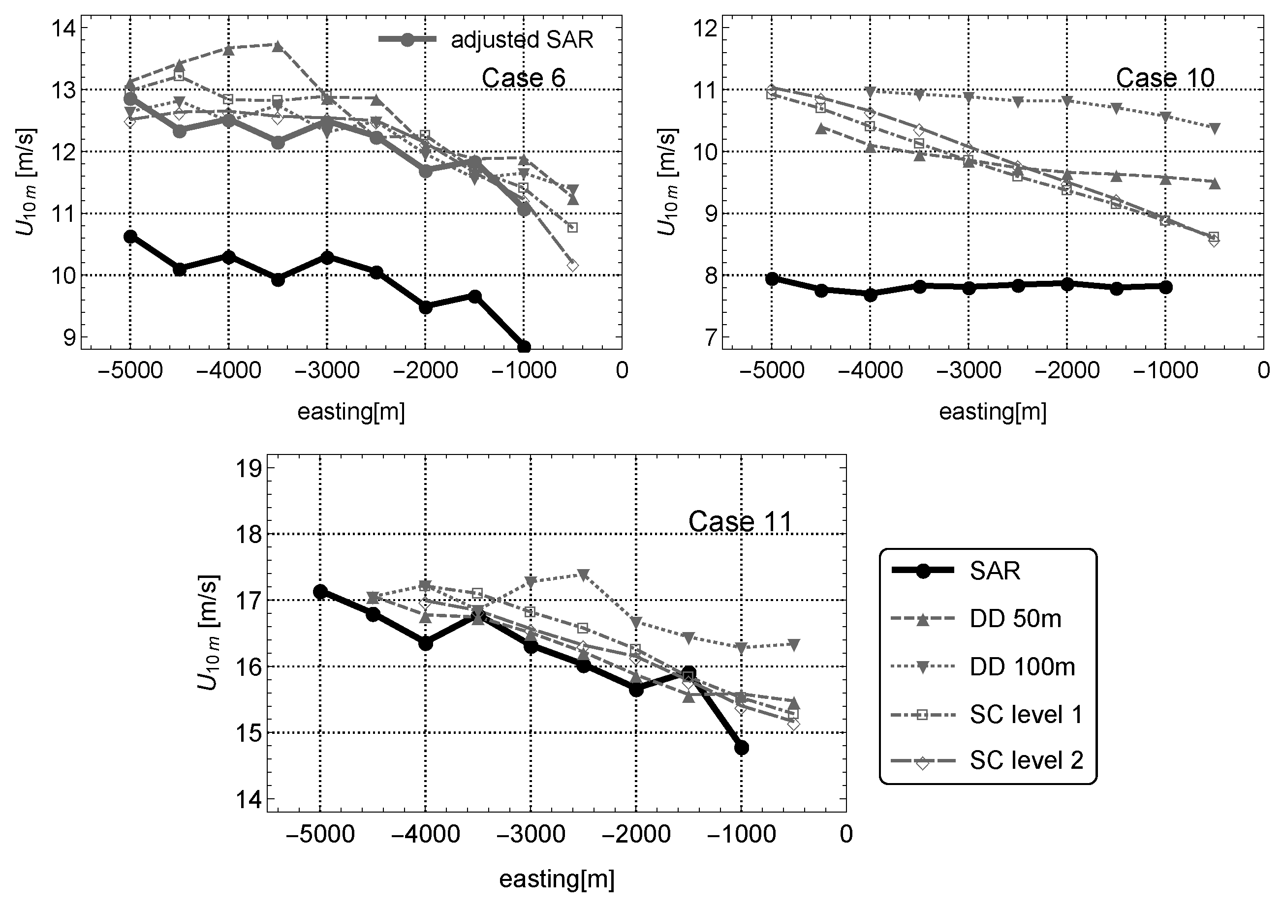
Figure 8.
Extra Wide Swath mode SAR wind map for case 6. Wind direction inputs are taken from a global GFS model with 0.25 resolution and 6 h time steps rather than a fixed wind direction. The black star indicates the position of the RUNE experiment and the entire campaign area lies in the first subswath furthest East.

Table 1.
Overview of selected previous studies on the accuracy of C-band SAR wind retrievals.
| Reference | Samples | Location | RMSE () | Sensor |
|---|---|---|---|---|
| Hasager et al. [9] | 149 to 197 | Denmark/The Netherlands | 1.27 to 1.65 | Envisat |
| Chang et al. [10] | 552 | South Chinese Sea | 2.09 | Envisat |
| Takeyama et al. [11] | 42 | Japan | 0.75 to 2.24 | Envisat |
| Chang et al. [12] | 522 | East Chinese Sea | 1.99 | Envisat |
| Takeyama et al. [13] | 33 to 73 | Japan | 0.64 to 2.34 | Envisat |
| Hasager et al. [14] | 875 | Baltic Sea | 1.17 | Envisat |
| Christiansen et al. [15] | 91 | Denmark | 1.1 to 1.8 | ERS2 |
| Hasager et al. [16] | 61 | Denmark | 0.9 to 1.14 | ERS2 |
Table 2.
SAR images available with at least one collocated LiDAR scan. The time is given in UTC. Polarization (Pol.) of the images, Modes: EW for extra wide swath and IW for interferometric wide swath, Orbit: D for descending and A for ascending. is the approximate incidence angle for the investigated area.
| Case | Date | Time | Pol. | Mode | Orbit | |
|---|---|---|---|---|---|---|
| 1 | 7 December 2015 | 17:09 | HH | EW | D | 37 |
| 2 | 9 December 2015 | 05:40 | VV | EW | A | 43 |
| 3 | 12 December 2015 | 17:17 | VV | IW | D | 44 |
| 4 | 14 December 2015 | 05:48 | HH | EW | A | 36 |
| 5 | 26 December 2015 | 05:48 | HH | IW | A | 36 |
| 6 | 31 December 2015 | 05:56 | HH | IW | D | 27 |
| 7 | 31 December 2015 | 17:09 | HH | IW | D | 37 |
| 8 | 12 January 2016 | 17:09 | HH | EW | A | 37 |
| 9 | 19 January 2016 | 05:48 | VV | EW | A | 36 |
| 10 | 26 January 2016 | 05:40 | VV | EW | D | 43 |
| 11 | 29 January 2016 | 17:17 | HH | EW | D | 44 |
| 12 | 5 February 2016 | 17:09 | HH | EW | D | 37 |
| 13 | 12 February 2016 | 05:48 | VV | IW | A | 36 |
| 14 | 17 February 2016 | 17:09 | HH | IW | D | 37 |
| 15 | 29 February 2016 | 05:57 | HH | EW | A | 27 |
Table 3.
Table of all cases with available SAR image and LiDAR measurements: dual Doppler (DD) and sector scans (SC), cases 14 and 15 have horizontal scans at 26 m. Wind speed ((50 m)) and direction ((50 m)) from the LiDAR at position P. Stability expressed in the Obukov length L is classified at the Høvsøre met mast at 40 m: very stable, m stable, neutral. Case 4 has wind speed and direction taken from Høvøre and the stability interpolated between 10 m and 60 m. For case 9 stability information was not reliable due to wind turbine wakes.
| Case | DD | SC | m | (40 m) (m) | Stab Class | |
|---|---|---|---|---|---|---|
| 1 | x | 7.5 | 148.5 | 40 | very stable | |
| 2 | x | 13.6 | 277 | 1320 | neutral | |
| 3 | x | 5.2 | 234 | 123 | stable | |
| 4 | x | 4.7 | H:167 | 50 | very stable | |
| 5 | x | x | 5.0 | 80 | 31 | very stable |
| 6 | x | x | 13.0 | 149 | −1480 | neutral |
| 7 | x | 10.0 | 205 | 46 | very stable | |
| 8 | x | x | 10.5 | 56 | 596.5 | neutral |
| 9 | x | x | 7.3 | 347 | - | - |
| 10 | x | x | 11.5 | 264 | 175 | stable |
| 11 | x | x | 19.0 | 250 | 1001 | neutral |
| 12 | x | x | 10.0 | 213 | 53 | very stable |
| 13 | x | x | 6.4 | 40 | 39 | very stable |
| 14 | x | 8.3 | 141 | 41 | very stable | |
| 15 | x | 4 | 133 | 43 | very stable |
Table 4.
Influence of the bin size along the coast on the average of the SAR wind retrieval. Number of SAR resolution cells included, mean and absolute mean of the differences from SAR winds only. The RMSE is given for preliminary comparisons of SAR and dual Doppler.
Table 4.
Influence of the bin size along the coast on the average of the SAR wind retrieval. Number of SAR resolution cells included, mean and absolute mean of the differences from SAR winds only. The RMSE is given for preliminary comparisons of SAR and dual Doppler.
| - | 1 km | 1.5 km | 2 km | 3 km | |
|---|---|---|---|---|---|
| Cells (-) | 1 | 2 | 3 | 4 | 6 |
| (ms) | - | −0.01 | −0.02 | −0.03 | −0.04 |
| (ms) | - | 0.18 | 0.21 | 0.24 | 0.28 |
| RMSE () | 1.53 | 1.45 | 1.41 | 1.42 | 1.43 |
Table 5.
Mean bias and median, minimum and maximum standard deviations for binned wind speed differences between SAR and scanning LiDARs in Figure 3 for dual Doppler and sector scan.
Table 5.
Mean bias and median, minimum and maximum standard deviations for binned wind speed differences between SAR and scanning LiDARs in Figure 3 for dual Doppler and sector scan.
| Mean Bias (ms) | Median STD (ms) | Min STD (ms) | Max STD () | |
|---|---|---|---|---|
| DD | −0.57 | 1.30 | 1.07 | 1.62 |
| SC | −0.17 | 1.47 | 1.17 | 1.98 |
© 2017 by the authors. Licensee MDPI, Basel, Switzerland. This article is an open access article distributed under the terms and conditions of the Creative Commons Attribution (CC BY) license (http://creativecommons.org/licenses/by/4.0/).
Share and Cite
MDPI and ACS Style
Ahsbahs, T.; Badger, M.; Karagali, I.; Larsén, X.G. Validation of Sentinel-1A SAR Coastal Wind Speeds Against Scanning LiDAR. Remote Sens. 2017, 9, 552. https://doi.org/10.3390/rs9060552
AMA Style
Ahsbahs T, Badger M, Karagali I, Larsén XG. Validation of Sentinel-1A SAR Coastal Wind Speeds Against Scanning LiDAR. Remote Sensing. 2017; 9(6):552. https://doi.org/10.3390/rs9060552
Chicago/Turabian StyleAhsbahs, Tobias, Merete Badger, Ioanna Karagali, and Xiaoli Guo Larsén. 2017. "Validation of Sentinel-1A SAR Coastal Wind Speeds Against Scanning LiDAR" Remote Sensing 9, no. 6: 552. https://doi.org/10.3390/rs9060552
Note that from the first issue of 2016, this journal uses article numbers instead of page numbers. See further details here.