
Multi-Algorithm Indices and Look-Up Table for Chlorophyll-a Retrieval in Highly Turbid Water Bodies Using Multispectral Data

 ,
,  ,
,
Abstract
:
1. Introduction
2. Methods
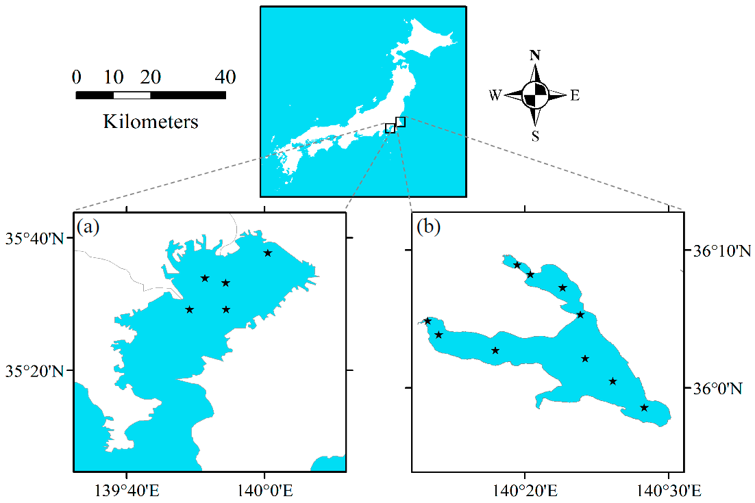
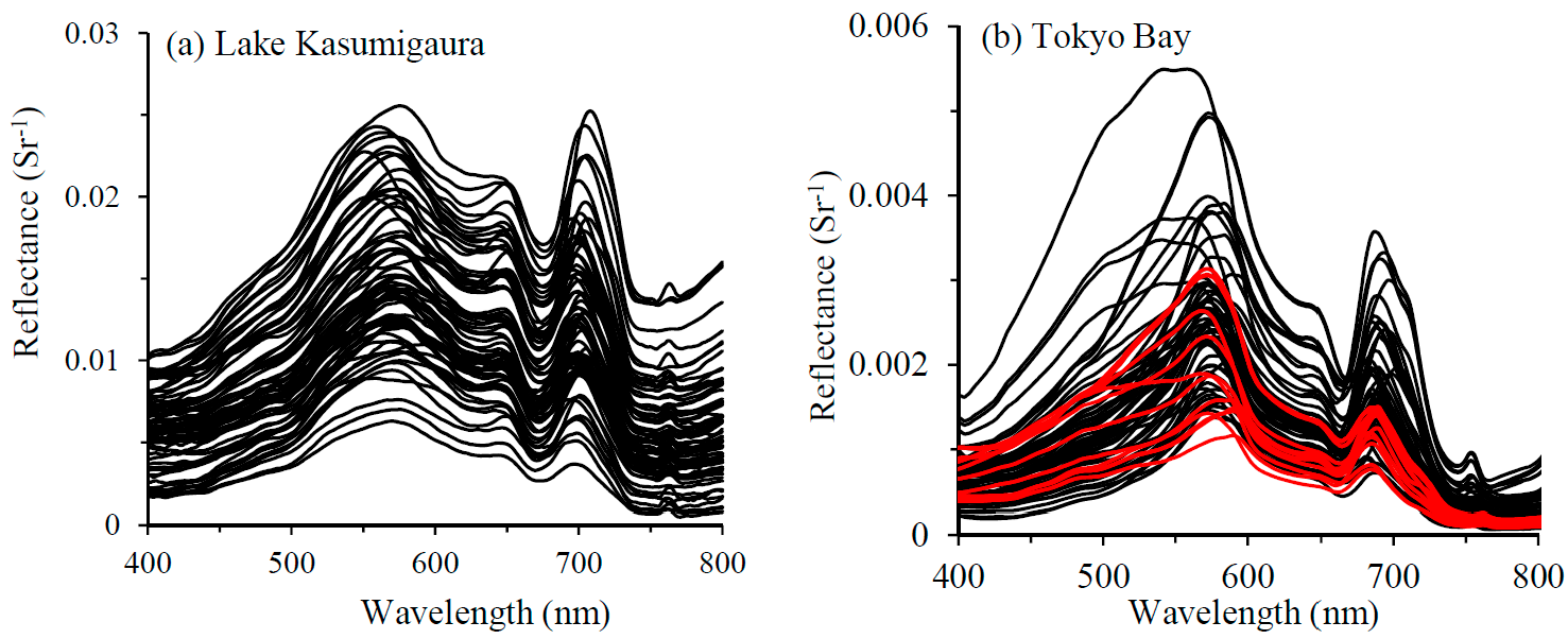
2.1. In Situ and Laboratory Measurements
2.2. Bio-Optical Model
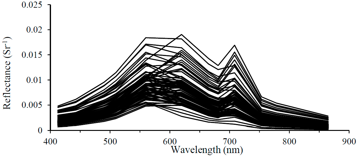
2.3. Simulating the Remote Sensing Reflectance
2.4. MERIS Images Processing
2.5. Accuracy Assessment of the Algorithms
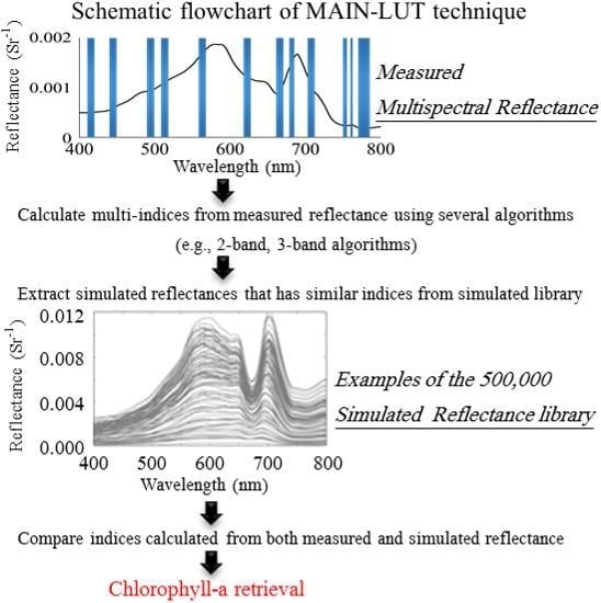
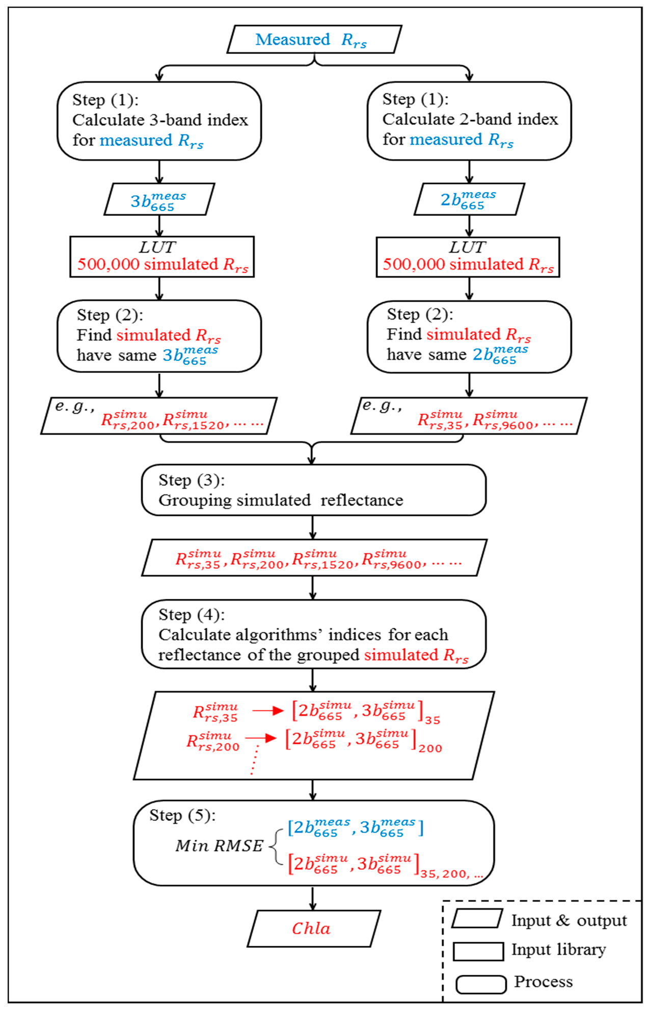
3. Construction of the Multi-Algorithm Indices and Look-Up Table (MAIN-LUT)
- Step (0)
- two things should be prepared and selected before using MAIN-LUT: (1) a library of simulated Rrs should be provided through a look-up table; and (2) one combination of algorithms should be selected from Table 4. The selected combination is hereafter called Sample Combination through the coming steps.
- Step (1)
- calculating algorithms indices for the measured reflectance using Equations (15)–(18). The number of required indices relies on the selection of the Sample Combination in Step (0). For example, the 2-indices-[665] combination was selected in the flowchart (Figure 5). As a result, the indices of 2b-[665, 709] and 3b-[665, 709, 754] algorithms were estimated as and as shown in Figure 5.
- Step (2)
- for each measured index estimated in Step (1), simulated reflectance spectra from a look-up table (LUT) that have the same index should be extracted. Of course, many simulated reflectance spectra with different tagged Chla will be extracted from this matching process. For example, the simulated reflectance (, ) were extracted because they matched the . The 200 and 1520 represent the tagged numbers of simulated reflectance for a certain combination of Chla, NAP, and CDOM and these tagged numbers range from 1 to 500,000.
- Step (3)
- grouping of simulated reflectance extracted from Step (2), which was generated from the matching process of each measured index.
- Step (4)
- estimating algorithm indices for each of simulated reflectance grouped in Step (3). The number of required indices is based on the Sample Combination selected in Step (0).
- Step (5)
- The RMSE is used to compare the indices of measured reflectance with simulated indices of each extracted reflectance in Step (3) as follows:where denote measured indices (i.e., and for 2b-indices-[665] combination); refer to simulated indices calculated for each simulated Rrs spectrum (i.e., and for 2b-indices-[665] combination), j is an index for simulated reflectance grouped in Step (3); and n represents the number of indices in the Sample Combination (i.e., n = 2 for 2b-indices-[665] combination). The minimum RMSE value represents the closest simulated spectrum from the measured spectrum. As a result, the tagged Chla for that simulated Rrs will be the retrieved Chla concentration of the measured Rrs.
4. Results and Discussion
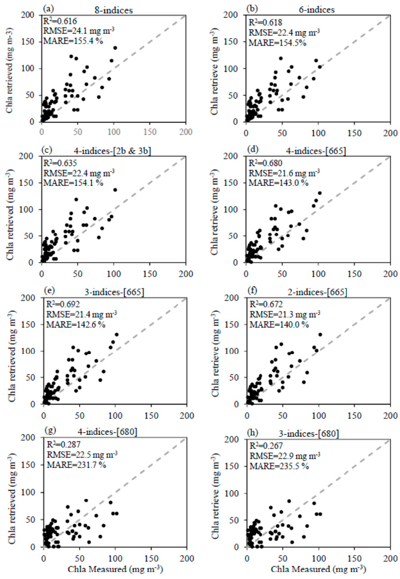
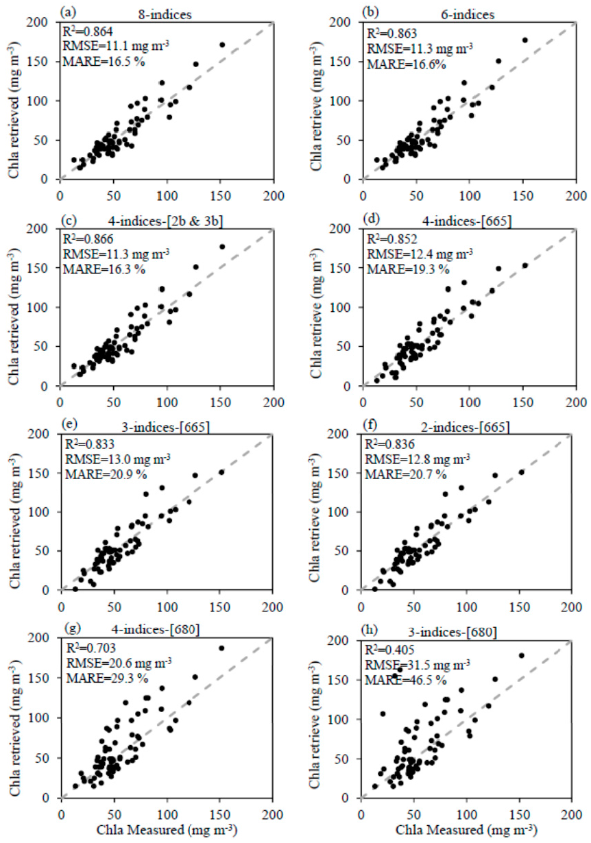
4.1. Validation Using In Situ Measurements
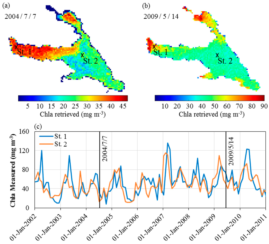
4.2. Validation Using MERIS Data
4.3. Comparing MAIN-LUT with Locally Tuned Algorithms
5. Conclusions
Supplementary Materials
Acknowledgments
Author Contributions
Conflicts of Interest
References
- Tyler, A.N.; Hunter, P.D.; Spyrakos, E.; Groom, S.; Constantinescu, A.M.; Kitchen, J. Developments in Earth observation for the assessment and monitoring of inland, transitional, coastal and shelf-sea waters. Sci. Total Environ. 2016, 572, 1307–1321. [Google Scholar] [CrossRef] [PubMed]
- Bresciani, M.; Stroppiana, D.; Odermatt, D.; Morabito, G.; Giardino, C. Assessing remotely sensed chlorophyll-a for the implementation of the Water Framework Directive in European perialpine lakes. Sci. Total Environ. 2011, 409, 3083–3091. [Google Scholar] [CrossRef] [PubMed]
- Shi, K.; Zhang, Y.; Liu, X.; Wang, M.; Qin, B. Remote sensing of diffuse attenuation coefficient of photosynthetically active radiation in Lake Taihu using MERIS data. Remote Sens. Environ. 2014, 140, 365–377. [Google Scholar] [CrossRef]
- Austin, R.W.; Petzold, T.J. The Determination of the Diffuse Attenuation Coefficient of Sea Water Using the Coastal Zone Color Scanner. In Oceanography from Space; Barale, V., Gower, J.F.R., Alberotanza, L., Eds.; Springer: Boston, MA, USA, 1981; pp. 239–256. [Google Scholar]
- Yoder, J.A.; McClain, C.R.; Blanton, J.O.; Oeymay, L.-Y. Spatial scales in CZCS-chlorophyll imagery of the southeastern U.S. continental shelf1. Limnol. Oceanogr. 1987, 32, 929–941. [Google Scholar] [CrossRef]
- International Ocean Colour Coordinating Group (IOCCG). Remote Sensing of Inherent Optical Properties: Fundamentals, Tests of Algorithms, and Applications; Lee, Z.-P., Ed.; Reports of the International Ocean Colour Coordinating Group; IOCCG: Dartmouth, NS, Canada, 2006; Volume 5. [Google Scholar]
- International Ocean Colour Coordinating Group (IOCCG). Phytoplankton Functional Types from Space; Sathyendranath, S., Ed.; Reports of the International Ocean Colour Coordinating Group; IOCCG: Dartmouth, NS, Canada, 2014; Volume 15. [Google Scholar]
- International Ocean Colour Coordinating Group (IOCCG). Atmospheric Correction for Remotely-Sensed Ocean-Colour Products; Reports of the International Ocean Colour Coordinating Group; Wang, M., Ed.; IOCCG: Dartmouth, NS, Canada, 2010; Volume 10. [Google Scholar]
- Kutser, T. Quantitative detection of chlorophyll in cyanobacterial blooms by satellite remote sensing. Limnol. Oceanogr. 2004, 49, 2179–2189. [Google Scholar] [CrossRef]
- Majozi, N.P.; Salama, M.S.; Bernard, S.; Harper, D.M.; Habte, M.G. Remote sensing of euphotic depth in shallow tropical inland waters of Lake Naivasha using MERIS data. Remote Sens. Environ. 2014, 148, 178–189. [Google Scholar] [CrossRef]
- Mishra, S.; Mishra, D.R. Normalized difference chlorophyll index: A novel model for remote estimation of chlorophyll-a concentration in turbid productive waters. Remote Sens. Environ. 2012, 117, 394–406. [Google Scholar] [CrossRef]
- Matsushita, B.; Yang, W.; Chang, P.; Yang, F.; Fukushima, T. A simple method for distinguishing global Case-1 and Case-2 waters using SeaWiFS measurements. ISPRS J. Photogramm. Remote Sens. 2012, 69, 74–87. [Google Scholar] [CrossRef]
- Lee, Z.; Carder, K.L.; Arnone, R.A. Deriving Inherent Optical Properties from Water Color: A Multiband Quasi-Analytical Algorithm for Optically Deep Waters. Appl. Opt. 2002, 41, 5755. [Google Scholar] [CrossRef] [PubMed]
- Garver, S.A.; Siegel, D.A. Inherent optical property inversion of ocean color spectra and its biogeochemical interpretation: 1. Time series from the Sargasso Sea. J. Geophys. Res. Ocean. 1997, 102, 18607–18625. [Google Scholar] [CrossRef]
- O’Reilly, J.E.; Maritorena, S.; Mitchell, B.G.; Siegel, D.A.; Carder, K.L.; Garver, S.A.; Kahru, M.; McClain, C. Ocean color chlorophyll algorithms for SeaWiFS. J. Geophys. Res. 1998, 103, 24937. [Google Scholar] [CrossRef]
- Li, L.; Li, L.; Song, K.; Li, Y.; Tedesco, L.P.; Shi, K.; Li, Z. An inversion model for deriving inherent optical properties of inland waters: Establishment, validation and application. Remote Sens. Environ. 2013, 135, 150–166. [Google Scholar] [CrossRef]
- Song, K.; Li, L.; Tedesco, L.P.P.; Li, S.; Duan, H.; Liu, D.; Hall, B.E.E.; Du, J.; Li, Z.; Shi, K.; Zhao, Y. Remote estimation of chlorophyll-a in turbid inland waters: Three-band model versus GA-PLS model. Remote Sens. Environ. 2013, 136, 342–357. [Google Scholar] [CrossRef]
- Sun, D.; Li, Y.; Le, C.; Shi, K.; Huang, C.; Gong, S.; Yin, B. A semi-analytical approach for detecting suspended particulate composition in complex turbid inland waters (China). Remote Sens. Environ. 2013, 134, 92–99. [Google Scholar] [CrossRef]
- Yang, W.; Matsushita, B.; Chen, J.; Fukushima, T. A Relaxed Matrix Inversion Method for Retrieving Water Constituent Concentrations in Case II Waters: The Case of Lake Kasumigaura, Japan. IEEE Trans. Geosci. Remote Sens. 2011, 49, 3381–3392. [Google Scholar] [CrossRef]
- Han, L.; Rundquist, D.C.; Liu, L.L.; Fraser, R.N.; Schalles, J.F. The spectral responses of algal chlorophyll in water with varying levels of suspended sediment. Int. J. Remote Sens. 1994, 15, 3707–3718. [Google Scholar] [CrossRef]
- Gons, H.J. Optical Teledetection of Chlorophyll a in Turbid Inland Waters. Environ. Sci. Technol. 1999, 33, 1127–1132. [Google Scholar] [CrossRef]
- Oki, K.; Yasuoka, Y. Estimation of Chlorophyll-a Concentration in Rich Chlorophyll Water Area from Near-infrared and Red Spectral Signature. J. Remote Sens. Soc. Jpn. 1996, 16, 315–323. [Google Scholar]
- Oki, K.; Yasuoka, Y. Estimation of Chlorophyll Concentration in Lakes and Inland Seas with a Field Spectroradiometer above the Water Surface. Appl. Opt. 2002, 41, 6463. [Google Scholar] [CrossRef] [PubMed]
- Dall’Olmo, G.; Gitelson, A.A.; Rundquist, D.C. Towards a unified approach for remote estimation of chlorophyll-a in both terrestrial vegetation and turbid productive waters. Geophys. Res. Lett. 2003, 30, 1938. [Google Scholar] [CrossRef]
- Le, C.; Li, Y.; Zha, Y.; Sun, D.; Huang, C.; Lu, H. A four-band semi-analytical model for estimating chlorophyll a in highly turbid lakes: The case of Taihu Lake, China. Remote Sens. Environ. 2009, 113, 1175–1182. [Google Scholar] [CrossRef]
- Lyu, H.; Li, X.; Wang, Y.; Jin, Q.; Cao, K.; Wang, Q.; Li, Y. Evaluation of chlorophyll-a retrieval algorithms based on MERIS bands for optically varying eutrophic inland lakes. Sci. Total Environ. 2015, 530–531, 373–382. [Google Scholar] [CrossRef] [PubMed]
- Lee, Z.; Carder, K.L.; Mobley, C.D.; Steward, R.G.; Patch, J.S. Hyperspectral remote sensing for shallow waters: 2 Deriving bottom depths and water properties by optimization. Appl. Opt. 1999, 38, 3831. [Google Scholar] [CrossRef] [PubMed]
- Klonowski, W.M.; Fearns, P.R.; Lynch, M.J. Retrieving key benthic cover types and bathymetry from hyperspectral imagery. J. Appl. Remote Sens. 2007, 1, 11505. [Google Scholar] [CrossRef]
- Hedley, J.; Roelfsema, C.; Phinn, S.R. Efficient radiative transfer model inversion for remote sensing applications. Remote Sens. Environ. 2009, 113, 2527–2532. [Google Scholar] [CrossRef]
- Brando, V.E.; Anstee, J.M.; Wettle, M.; Dekker, A.G.; Phinn, S.R.; Roelfsema, C. A physics based retrieval and quality assessment of bathymetry from suboptimal hyperspectral data. Remote Sens. Environ. 2009, 113, 755–770. [Google Scholar] [CrossRef]
- Louchard, E.M.; Reid, R.P.; Stephens, F.C.; Davis, C.O.; Leathers, R.A.; Downes, T.V. Optical Remote Sensing of Benthic Habitats and Bathymetry in Coastal Environments at Lee Stocking Island, Bahamas: A Comparative Spectral Classification Approach; DTIC: Fort Belvoir, VA, USA, 2002. [Google Scholar]
- Mobley, C.D.; Sundman, L.K.; Davis, C.O.; Bowles, J.H.; Downes, T.V.; Leathers, R.A.; Montes, M.J.; Bissett, W.P.; Kohler, D.D.R.; Reid, R.P.; et al. Interpretation of hyperspectral remote-sensing imagery by spectrum matching and look-up tables. Appl. Opt. 2005, 44, 3576. [Google Scholar] [CrossRef] [PubMed]
- Doerffer, R.; Helmut, S. Neural network for retrieval of concentrations of water constituents with the possibility of detecting exceptional out of scope spectra. In Proceedings of the IGARSS 2000: IEEE 2000 International Geoscience and Remote Sensing Symposium, Honolulu, HI, USA, 24–28 July 2000; IEEE: Piscataway, NJ, USA, 2000; Volume 2, pp. 714–717. [Google Scholar]
- Baruah, P.J.; Tamura, M.; Oki, K.; Nishimura, H. Neural network modeling of lake surface chlorophyll and sediment content from Landsat TM imagery. In Proceedings of the Paper presented at the 22nd Asian Conference on Remote Sensing, Singapore, 5–9 November 2001; Volume 5, p. 9. [Google Scholar]
- Doerffer, R.; Schiller, H. The MERIS Case 2 water algorithm. Int. J. Remote Sens. 2007, 28, 517–535. [Google Scholar] [CrossRef]
- Shen, F.; Zhou, Y.-X.; Li, D.-J.; Zhu, W.-J.; Suhyb Salama, M. Medium resolution imaging spectrometer (MERIS) estimation of chlorophyll-a concentration in the turbid sediment-laden waters of the Changjiang (Yangtze) Estuary. Int. J. Remote Sens. 2010, 31, 4635–4650. [Google Scholar] [CrossRef]
- Zhang, F.; Li, J.; Shen, Q.; Zhang, B.; Wu, C.; Wu, Y.; Wang, G.; Wang, S.; Lu, Z. Algorithms and Schemes for Chlorophyll a Estimation by Remote Sensing and Optical Classification for Turbid Lake Taihu, China. IEEE J. Sel. Top. Appl. Earth Obs. Remote Sens. 2015, 8, 350–364. [Google Scholar] [CrossRef]
- Oki, K. Why is the Ratio of Reflectivity Effective for Chlorophyll Estimation in the Lake Water? Remote Sens. 2010, 2, 1722–1730. [Google Scholar] [CrossRef]
- Carder, K.L.; Chen, F.R.; Lee, Z.P.; Hawes, S.K.; Kamykowski, D. Semianalytic Moderate-Resolution Imaging Spectrometer algorithms for chlorophyll a and absorption with bio-optical domains based on nitrate-depletion temperatures. J. Geophys. Res. 1999, 104, 5403. [Google Scholar] [CrossRef]
- Huang, Y.; Jiang, D.; Zhuang, D.; Fu, J. Evaluation of hyperspectral indices for chlorophyll-a concentration estimation in Tangxun Lake (Wuhan, China). Int. J. Environ. Res. Public Health 2010, 7, 2437–2451. [Google Scholar] [CrossRef] [PubMed]
- Zhou, L.; Roberts, D.A.; Ma, W.; Zhang, H.; Tang, L. Estimation of higher chlorophylla concentrations using field spectral measurement and HJ-1A hyperspectral satellite data in Dianshan Lake, China. ISPRS J. Photogramm. Remote Sens. 2014, 88, 41–47. [Google Scholar] [CrossRef]
- Shi, K.; Li, Y.; Li, L.; Lu, H.; Song, K.; Liu, Z.; Xu, Y.; Li, Z. Remote chlorophyll-a estimates for inland waters based on a cluster-based classification. Sci. Total Environ. 2013, 444, 1–15. [Google Scholar] [CrossRef] [PubMed]
- Gurlin, D.; Gitelson, A.A.; Moses, W.J. Remote estimation of chl-a concentration in turbid productive waters—Return to a simple two-band NIR-red model? Remote Sens. Environ. 2011, 115, 3479–3490. [Google Scholar] [CrossRef]
- Matsushita, B.; Yang, W.; Yu, G.; Oyama, Y.; Yoshimura, K.; Fukushima, T. A hybrid algorithm for estimating the chlorophyll-a concentration across different trophic states in Asian inland waters. ISPRS J. Photogramm. Remote Sens. 2015, 102, 28–37. [Google Scholar] [CrossRef]
- Kutser, T.; Metsamaa, L.; Strömbeck, N.; Vahtmäe, E. Monitoring cyanobacterial blooms by satellite remote sensing. Estuar. Coast. Shelf Sci. 2006, 67, 303–312. [Google Scholar] [CrossRef]
- Matthews, M.W. A current review of empirical procedures of remote sensing in inland and near-coastal transitional waters. Int. J. Remote Sens. 2011, 32, 6855–6899. [Google Scholar] [CrossRef]
- Yang, W.; Matsushita, B.; Chen, J.; Fukushima, T. Estimating constituent concentrations in case II waters from MERIS satellite data by semi-analytical model optimizing and look-up tables. Remote Sens. Environ. 2011, 115, 1247–1259. [Google Scholar] [CrossRef]
- Lee, Z.; Carder, K.L.; Mobley, C.D.; Steward, R.G.; Patch, J.S. Hyperspectral remote sensing for shallow waters. I. A semianalytical model. Appl. Opt. 1998, 37, 6329–6338. [Google Scholar] [CrossRef] [PubMed]
- Giardino, C.; Brando, V.E.; Dekker, A.G.; Strömbeck, N.; Candiani, G. Assessment of water quality in Lake Garda (Italy) using Hyperion. Remote Sens. Environ. 2007, 109, 183–195. [Google Scholar] [CrossRef]
- Lyons, M.; Phinn, S.; Roelfsema, C. Integrating Quickbird Multi-Spectral Satellite and Field Data: Mapping Bathymetry, Seagrass Cover, Seagrass Species and Change in Moreton Bay, Australia in 2004 and 2007. Remote Sens. 2011, 3, 42–64. [Google Scholar] [CrossRef]
- Lee, Z.; Carder, K.L.; Chen, R.F.; Peacock, T.G. Properties of the water column and bottom derived from Airborne Visible Infrared Imaging Spectrometer (AVIRIS) data. J. Geophys. Res. Ocean. 2001, 106, 11639–11651. [Google Scholar] [CrossRef]
- Schueler, C.; Yoder, J.; Antoine, D.; Castillo, C.; Evans, R.; Mengelt, C.; Mobley, C.; Sarmiento, J.; Sathyendranath, S.; Siegel, D.; et al. Assessing Requirements for Sustained Ocean Color Research and Observations. In Proceedings of the AIAA SPACE 2011 Conference & Exposition, Long Beach, CA, USA, 27–29 September 2011; American Institute of Aeronautics and Astronautics: Reston, VA, USA, 2011. [Google Scholar]
- Dekker, A.G.; Phinn, S.R.; Anstee, J.; Bissett, P.; Brando, V.E.; Casey, B.; Fearns, P.; Hedley, J.; Klonowski, W.; Lee, Z.P. Intercomparison of shallow water bathymetry, hydro-optics, and benthos mapping techniques in Australian and Caribbean coastal environments. Limnol. Oceanogr. Methods 2011, 9, 396–425. [Google Scholar] [CrossRef]
- Dalponte, M.; Bruzzone, L.; Gianelle, D. Tree species classification in the Southern Alps based on the fusion of very high geometrical resolution multispectral/hyperspectral images and LiDAR data. Remote Sens. Environ. 2012, 123, 258–270. [Google Scholar] [CrossRef]
- Lesser, M.P.; Mobley, C.D. Bathymetry, water optical properties, and benthic classification of coral reefs using hyperspectral remote sensing imagery. Coral Reefs 2007, 26, 819–829. [Google Scholar] [CrossRef]
- NIES Lake Kasumigaura Database, National Institute for Environmental Studies, Japan. Available online: http://db.cger.nies.go.jp/gem/moni-e/inter/GEMS/database/kasumi/index.html (accessed on 20 November 2016).
- Welschmeyer, N.A. Fluorometric analysis of chlorophyll a in the presence of chlorophyll b and pheopigments. Limnol. Oceanogr. 1994, 39, 1985–1992. [Google Scholar] [CrossRef]
- Suzuki, R.; Ishimaru, T. An improved method for the determination of phytoplankton chlorophyll using N, N-dimethylformamide. J. Oceanogr. Soc. Jpn. 1990, 46, 190–194. [Google Scholar] [CrossRef]
- American Public Health Association. Standard Methods for the Examination of Water and Wastewater; American Public Health Association: Washington, DC, USA, 2005. [Google Scholar]
- Mobley, C.D. Estimation of the Remote-Sensing Reflectance from Above-Surface Measurements. Appl. Opt. 1999, 38, 7442–7448. [Google Scholar] [CrossRef] [PubMed]
- Mitchell, B.G.; Kahru, M.; Wieland, J.; Stramska, M.; Mueller, J.L. Determination of spectral absorption coefficients of particles, dissolved material and phytoplankton for discrete water samples. Ocean Opt. Protoc. Satell. Ocean Color Sens. Valid. Revis. 2002, 3, 231–257. [Google Scholar]
- Morel, A. Optical properties of pure water and pure sea water. Opt. Asp. Oceanogr. 1974, 1, 1–24. [Google Scholar]
- Dall’Olmo, G.; Gitelson, A.A. Effect of bio-optical parameter variability and uncertainties in reflectance measurements on the remote estimation of chlorophyll-a concentration in turbid productive waters: Modeling results. Appl. Opt. 2006, 45, 3577. [Google Scholar] [CrossRef] [PubMed]
- Mélin, F.; Vantrepotte, V.; Clerici, M.; D’Alimonte, D.; Zibordi, G.; Berthon, J.-F.; Canuti, E. Multi-sensor satellite time series of optical properties and chlorophyll-a concentration in the Adriatic Sea. Prog. Oceanogr. 2011, 91, 229–244. [Google Scholar] [CrossRef]
- Gordon, H.; Brown, J.; Brown, O.; Evans, R.; Smith, R. A semianalytic radiance model of ocean color. J. Geophys. Res. 1988, 93, 10909–10924. [Google Scholar] [CrossRef]
- Kirk, J.T.O. Dependence of relationship between inherent and apparent optical properties of water on solar altitude. Limnol. Oceanogr. 1984, 29, 350–356. [Google Scholar] [CrossRef]
- Buiteveld, H.; Hakvoort, J.H.M.; Donze, M. Optical properties of pure water. In Ocean Optics XII; Jaffe, J.S., Ed.; International Society for Optics and Photonics: Bellingham, WA, USA, 1994; pp. 174–183. [Google Scholar]
- Austin, R.W. Gulf of Mexico, ocean-color surface-truth measurements. Bound. Layer Meteorol. 1980, 18, 269–285. [Google Scholar] [CrossRef]
- Zhu, W.; Yu, Q.; Tian, Y.Q.; Becker, B.L.; Zheng, T.; Carrick, H.J. An assessment of remote sensing algorithms for colored dissolved organic matter in complex freshwater environments. Remote Sens. Environ. 2014, 140, 766–778. [Google Scholar] [CrossRef]
- Yang, W.; Matsushita, B.; Chen, J.; Yoshimura, K.; Fukushima, T. Retrieval of Inherent Optical Properties for Turbid Inland Waters From Remote-Sensing Reflectance. IEEE Trans. Geosci. Remote Sens. 2013, 51, 3761–3773. [Google Scholar] [CrossRef]
- Gilerson, A.; Zhou, J.; Hlaing, S.; Ioannou, I.; Schalles, J.; Gross, B.; Moshary, F.; Ahmed, S. Fluorescence component in the reflectance spectra from coastal waters. Dependence on water composition. Opt. Express 2007, 15, 15702–15721. [Google Scholar] [CrossRef] [PubMed]
- Oyama, Y.; Matsushita, B.; Fukushima, T.; Matsushige, K.; Imai, A. Application of spectral decomposition algorithm for mapping water quality in a turbid lake (Lake Kasumigaura, Japan) from Landsat TM data. ISPRS J. Photogramm. Remote Sens. 2009, 64, 73–85. [Google Scholar] [CrossRef]
- Gons, H.J.; Burger-Wiersma, T.; Otten, J.H.; Rijkeboer, M. Coupling of phytoplankton and detritus in a shallow, eutrophic lake (Lake Loosdrecht, The Netherlands). Hydrobiologia 1992, 233, 51–59. [Google Scholar] [CrossRef]
- Gower, J.F.R.; Doerffer, R.; Borstad, G.A. Interpretation of the 685 nm peak in water-leaving radiance spectra in terms of fluorescence, absorption and scattering, and its observation by MERIS. Int. J. Remote Sens. 1999, 20, 1771–1786. [Google Scholar] [CrossRef]
- European Space Agency (ESA) Earthnet. Available Online: http://earth.esa.int/ (accessed on 10 March 2015).
- Binding, C.E.; Greenberg, T.A.; Jerome, J.H.; Bukata, R.P.; Letourneau, G. An assessment of MERIS algal products during an intense bloom in Lake of the Woods. J. Plankton Res. 2011, 33, 793–806. [Google Scholar] [CrossRef]
- Doerffer, R.; Schiller, H. MERIS Lake Water Algorithm for BEAM—MERIS Algorithm Theoretical Basis Document; V1.0, 10 June 2008; GKSS Research Center: Geesthacht, Germany, 2008. [Google Scholar]
- Egghe, L.; Leydesdorff, L. The relation between Pearson’s correlation coefficient r and Salton’s cosine measure. J. Am. Soc. Inf. Sci. Technol. 2009, 60, 1027–1036. [Google Scholar] [CrossRef]
- Moore, T.S.; Dowell, M.D.; Bradt, S.; Verdu, A.R. An optical water type framework for selecting and blending retrievals from bio-optical algorithms in lakes and coastal waters. Remote Sens. Environ. 2014, 143, 97–111. [Google Scholar] [CrossRef] [PubMed]
- Le, C.; Hu, C.; Cannizzaro, J.; English, D.; Muller-Karger, F.; Lee, Z. Evaluation of chlorophyll-a remote sensing algorithms for an optically complex estuary. Remote Sens. Environ. 2013, 129, 75–89. [Google Scholar] [CrossRef]
- Salem, S.I.; Higa, H.; Kim, H.; Kobayashi, H.; Oki, K.; Oki, T. Retrieval accuracy assessment of chlorophyll-a algorithms considering different trophic statuses and optimal bands. J. Gt. Lakes Res. 2017, in press. [Google Scholar]
- Gower, J.; King, S.; Borstad, G.; Brown, L. Detection of intense plankton blooms using the 709 nm band of the MERIS imaging spectrometer. Int. J. Remote Sens. 2005, 26, 2005–2012. [Google Scholar] [CrossRef]


| Min | Max | Mean | Median | SD | RSD (%) | |
|---|---|---|---|---|---|---|
| Tokyo Bay (n = 71) | ||||||
| Chla (mg m−3) | 0.76 | 102.07 | 25.14 | 13.94 | 25.85 | 102.82 |
| TSS (g m−3) | 2.99 | 26.29 | 8.29 | 7.99 | 0.49 | 5.87 |
| Tokyo Bay with IOPs (n = 12) | ||||||
| Chla (mg m−3) | 2.9 | 42.6 | 18.31 | 11.85 | 14.99 | 81.87 |
| TSS (g m−3) | 2.99 | 9.86 | 6.34 | 6.81 | 2.24 | 35.38 |
| ISS (g m−3) | 0.81 | 6.13 | 2.96 | 2.22 | 1.63 | 55.24 |
| OSS (g m−3) | 0.96 | 7.16 | 3.39 | 2.9 | 1.75 | 51.63 |
| aph(440) (m−1) | 0.23 | 1.03 | 0.65 | 0.6 | 0.27 | 41.3 |
| aNAP(440) (m−1) | 0.14 | 0.34 | 0.22 | 0.21 | 0.07 | 31.75 |
| aCDOM(440) (m−1) | 0.06 | 0.47 | 0.25 | 0.19 | 0.14 | 56.23 |
| bb,p(442) (m−1) | 0.01 | 0.04 | 0.02 | 0.03 | 0.01 | 41.16 |
| Lake Kasumigaura (Dataset 1) (n = 68) | ||||||
| Chla (mg m−3) | 13.16 | 152.14 | 55.86 | 48.16 | 26.59 | 47.60 |
| TSS (g m−3) | 9.40 | 57.10 | 21.71 | 18.25 | 9.44 | 43.50 |
| Lake Kasumigaura * (Dataset 2) (n = 77) | ||||||
| Chla (mg m−3) | 8.10 | 179.40 | 65.98 | 59.90 | 35.90 | 54.42 |
| TSS (g m−3) | 10.70 | 59.10 | 25.00 | 23.67 | 10.14 | 40.56 |
| Symbol | Description | Units |
|---|---|---|
| (Chla) | Chlorophyll-a concentration | mg m−3 |
| (NAP) | Non-algal particle concentration | g m−3 |
| (CDOM) | Colored dissolved organic matter absorption at 440 nm | m−1 |
| aw(λ) | Absorption coefficient of pure water | m−1 |
| aph(λ) | Absorption coefficient of phytoplankton | m−1 |
| aNAP(λ) | Absorption coefficient of NAP | m−1 |
| aCDOM(λ) | Absorption coefficient of CDOM | m−1 |
| a(λ) | Total absorption coefficient (=aw(λ) + aph(λ) + aNAP(λ) + aCDOM(λ)) | m−1 |
| bb,w(λ) | Backscattering coefficients of pure water | m−1 |
| bb,p(λ) | Backscattering coefficients of suspendedparticles | m−1 |
| bb,ph(λ) | Backscattering coefficients of phytoplankton | m−1 |
| bb,NAP(λ) | Backscattering coefficients of NAP | m−1 |
| bb(λ) | Total backscattering coefficient (=bb,w(λ) + bb,ph(λ) + bb,NAP(λ)) | m−1 |
| Rrs(λ) | Above-surface remote sensing reflectance | sr−1 |
| rrs(λ) | Subsurface remote sensing reflectance | sr−1 |
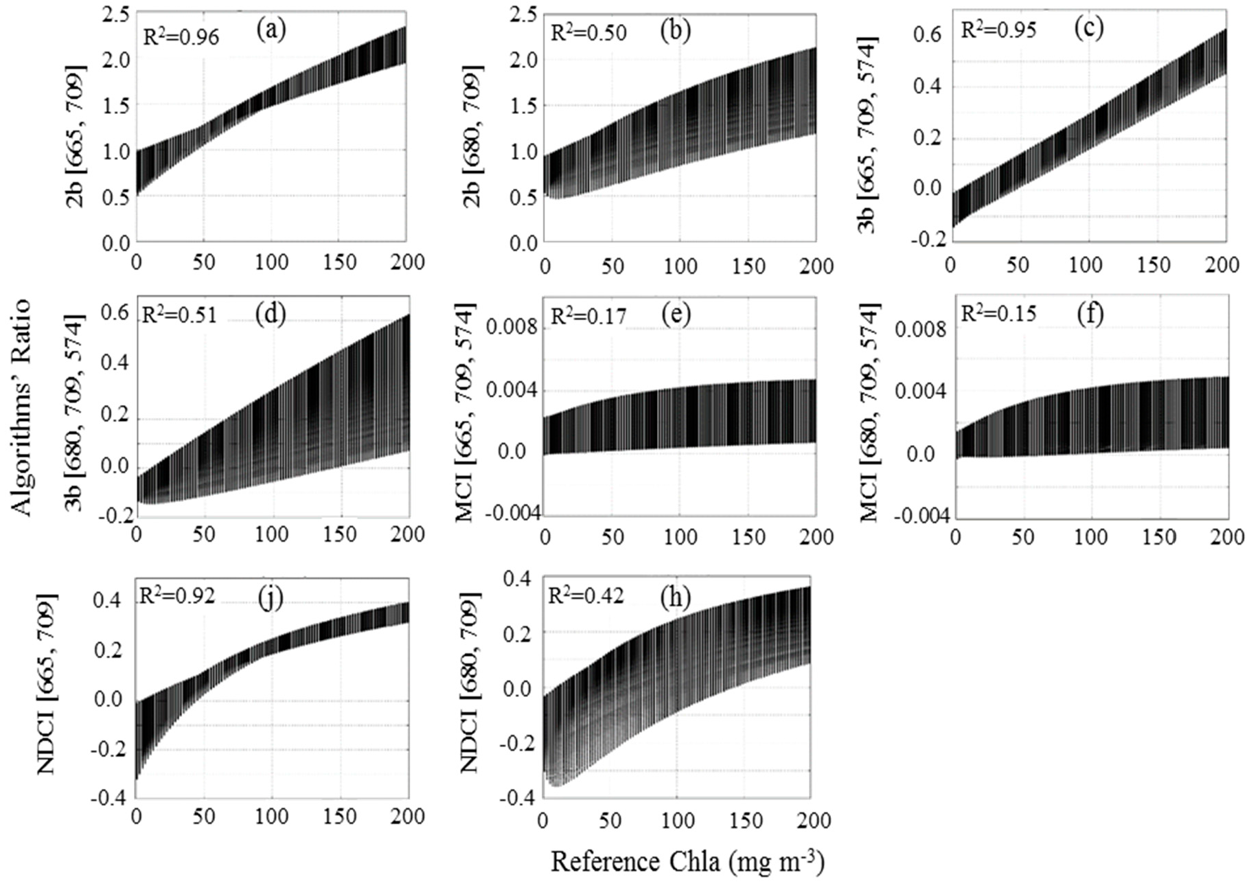
| No. | Algorithms | Algorithms’ Name | Wavelength | References | ||
|---|---|---|---|---|---|---|
| λ1 | λ2 | λ3 | ||||
| 1 | Two-band ratio | 2b [665, 709] | 665 | 709 | Gons [21] | |
| 2 | 2b [680, 709] | 680 | 709 | |||
| 3 | Three-band algorithm | 3b [665, 709, 754] | 665 | 709 | 754 | Dall’Olmo et al. [24] |
| 4 | 3b [680, 709, 754] | 680 | 709 | 754 | ||
| 5 | Maximum chlorophyll index | MCI [665, 709, 754] | 665 | 709 | 754 | Gower et al. [82] |
| 6 | MCI [680, 709, 754] | 680 | 709 | 754 | ||
| 7 | Normalized difference chlorophyll index | NDCI [665, 709, 754] | 665 | 709 | Mishra et al. [11] | |
| 8 | NDCI [680, 709, 754] | 680 | 709 | |||
| Algorithms’ Name * | ||||||||
|---|---|---|---|---|---|---|---|---|
| Algorithms’ Combinations | 2b [665, 709] | 2b [680, 709] | 3b [665, 709, 754] | 3b [680, 709, 754] | MCI [665, 709, 754] | MCI [680, 709, 754] | NDCI [665, 709] | NDCI [680, 709] |
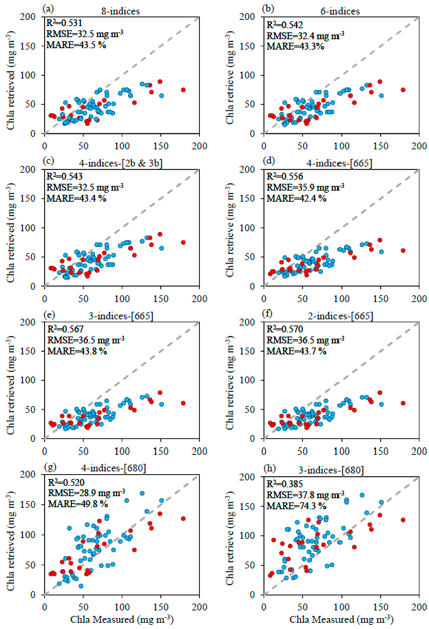
| 8-indices | ✓ | ✓ | ✓ | ✓ | ✓ | ✓ | ✓ | ✓ |
| 6-indices | ✓ | ✓ | ✓ | ✓ | ✓ | ✓ | ||
| 4-indices-[2b & 3b] | ✓ | ✓ | ✓ | ✓ | ||||
| 4-indices-[665] | ✓ | ✓ | ✓ | ✓ | ||||
| 3-indices-[665] | ✓ | ✓ | ✓ | |||||
| 2-indices-[665] | ✓ | ✓ | ||||||
| 4-indices-[680] | ✓ | ✓ | ✓ | ✓ | ||||
| 3-indices-[680] | ✓ | ✓ | ✓ | |||||
| Algorithms | Tokyo Bay (In Situ Data) | Lake Kasumigaura (Dataset 1) | Lake Kasumigaura (Dataset 2) | ||||||
|---|---|---|---|---|---|---|---|---|---|
| n = 49 | n = 47 | n = 53 | |||||||
| R2 | a0 | a1 | R2 | a0 | a1 | R2 | a0 | a1 | |
| 2b [665, 709] | 0.67 | 68.52 | −42.85 | 0.85 | 109.31 | −81.19 | 0.52 | 143.98 | −95.37 |
| 2b [680, 709] | 0.61 | 126.25 | −60.07 | 0.84 | 113.42 | −88.35 | 0.54 | 127.26 | −93.89 |
| 3b [665, 709, 754] | 0.60 | 235.05 | 26.32 | 0.91 | 267.05 | 26.95 | 0.52 | 490.74 | 43.67 |
| 3b [680, 709, 754] | 0.67 | 464.98 | 64.40 | 0.84 | 268.25 | 24.69 | 0.54 | 358.01 | 35.77 |
| MCI [665, 709, 754] | 0.66 | 55421.74 | 3.78 | 0.53 | 10289.16 | 10.44 | 0.06 | 7023.47 | 48.00 |
| MCI [680, 709, 754] | 0.65 | 94031.85 | 22.29 | 0.53 | 9633.17 | 18.75 | 0.07 | 6218.31 | 53.15 |
| NDCI [665, 709] | 0.61 | 130.19 | 27.76 | 0.83 | 273.10 | 24.10 | 0.48 | 356.96 | 48.64 |
| NDCI [680, 709] | 0.58 | 200.35 | 65.21 | 0.82 | 321.06 | 19.69 | 0.50 | 307.39 | 37.50 |
| Algorithms | Tokyo Bay (In Situ Data) | Lake Kasumigaura (Dataset 1) | Lake Kasumigaura (Dataset 2) | |||
|---|---|---|---|---|---|---|
| n = 22 | n = 21 | n = 24 | ||||
| R2 | RMSE | R2 | RMSE | R2 | RMSE | |
| 2b [665, 709] | 0.67 | 15.42 | 0.85 | 7.65 | 0.52 | 28.99 |
| 2b [680, 709] | 0.62 | 16.81 | 0.83 | 9.83 | 0.54 | 26.17 |
| 3b [665, 709, 754] | 0.58 | 19.24 | 0.89 | 8.49 | 0.52 | 28.61 |
| 3b [680, 709, 754] | 0.70 | 17.51 | 0.84 | 8.62 | 0.55 | 27.81 |
| MCI [665, 709, 754] | 0.68 | 15.35 | 0.51 | 23.93 | 0.08 | 33.96 |
| MCI [680, 709, 754] | 0.67 | 18.12 | 0.51 | 16.93 | 0.10 | 39.09 |
| NDCI [665, 709] | 0.63 | 14.04 | 0.84 | 9.51 | 0.50 | 19.70 |
| NDCI [680, 709] | 0.58 | 17.45 | 0.81 | 11.27 | 0.52 | 19.31 |
| MAIN-LUT | 0.69 | 21.40 | 0.85 | 11.3 | 0.57 | 36.50 |
© 2017 by the authors. Licensee MDPI, Basel, Switzerland. This article is an open access article distributed under the terms and conditions of the Creative Commons Attribution (CC BY) license (http://creativecommons.org/licenses/by/4.0/).
Share and Cite
Salem, S.I.; Higa, H.; Kim, H.; Kazuhiro, K.; Kobayashi, H.; Oki, K.; Oki, T. Multi-Algorithm Indices and Look-Up Table for Chlorophyll-a Retrieval in Highly Turbid Water Bodies Using Multispectral Data. Remote Sens. 2017, 9, 556. https://doi.org/10.3390/rs9060556
Salem SI, Higa H, Kim H, Kazuhiro K, Kobayashi H, Oki K, Oki T. Multi-Algorithm Indices and Look-Up Table for Chlorophyll-a Retrieval in Highly Turbid Water Bodies Using Multispectral Data. Remote Sensing. 2017; 9(6):556. https://doi.org/10.3390/rs9060556
Chicago/Turabian StyleSalem, Salem Ibrahim, Hiroto Higa, Hyungjun Kim, Komatsu Kazuhiro, Hiroshi Kobayashi, Kazuo Oki, and Taikan Oki. 2017. "Multi-Algorithm Indices and Look-Up Table for Chlorophyll-a Retrieval in Highly Turbid Water Bodies Using Multispectral Data" Remote Sensing 9, no. 6: 556. https://doi.org/10.3390/rs9060556