
Dynamic Data Filtering of Long-Range Doppler LiDAR Wind Speed Measurements


ForWind, Institute of Physics, University of Oldenburg, Küpkersweg 70, 26129 Oldenburg, Germany
*
Author to whom correspondence should be addressed.
Remote Sens. 2017, 9(6), 561; https://doi.org/10.3390/rs9060561
Submission received: 24 December 2016
/
Revised: 26 May 2017
/
Accepted: 31 May 2017
/
Published: 4 June 2017
Abstract
:Doppler LiDARs have become flexible and versatile remote sensing devices for wind energy applications. The possibility to measure radial wind speed components contemporaneously at multiple distances is an advantage with respect to meteorological masts. However, these measurements must be filtered due to the measurement geometry, hard targets and atmospheric conditions. To ensure a maximum data availability while producing low measurement errors, we introduce a dynamic data filter approach that conditionally decouples the dependency of data availability with increasing range. The new filter approach is based on the assumption of self-similarity, that has not been used so far for LiDAR data filtering. We tested the accuracy of the dynamic data filter approach together with other commonly used filter approaches, from research and industry applications. This has been done with data from a long-range pulsed LiDAR installed at the offshore wind farm ‘alpha ventus’. There, an ultrasonic anemometer located approximately 2.8 km from the LiDAR was used as reference. The analysis of around 1.5 weeks of data shows, that the error of mean radial velocity can be minimised for wake and free stream conditions.
1. Introduction
The basis of any empirical work, whether in the commercial or scientific context, is data that have been acquired through a measurement process. Recording measurement data needs a carefully planned measurement campaign, the selection of suitable instruments with sufficient resolution for the desired purpose and an adequate measurement period. In recent years, the scanning aerosol heterodyne Doppler LiDAR—hereafter LiDAR—has become a standard device when flexible, versatile measurements are needed that go beyond standard point measurements in the wind energy sector [1,2,3,4,5,6]. Due to the measurement method of pulsed devices, it is possible to capture a plurality of quasi-instantaneously measurements along the laser beam. The internal processing of the raw measurement data in commercial LiDAR systems can mainly be seen as a black box for standard users. Although the general principle is known [7], manufacturers tend not to publish their exact processing algorithms. Invalid measurement data are occurring due to device-dependent reasons, measuring-dependent influences such as hard targets, measurements outside of the permissible parameter range and those appearing for unknown reasons. Once the measurements are conducted, it is no longer possible to determine whether physical or technical reasons formed the source of errors [8]. Thus, seemingly random outliers can arise despite good measuring conditions. Independently of the objective of analysis, it is necessary to filter valid from invalid measurements to produce accurate results.
While the primary measurement value is the radial speed, the LiDAR devices measure the backscattering intensity as a secondary value. Based on the manufacture, the backscattering is calculated as carrier-to-noise-ratio (CNR), respectively signal-to-noise-ratio (SNR), that can be interpreted as a quality indicator for the calculation of the radial speed from the spectral raw data. Frehlich [9] state that the accuracy of the radial velocity determination decreases with decreasing mean CNR level. While this conclusion from Frehlich represent a stochastic statement, this does not imply that individual measurement points with low CNR values must be inaccurate or invalid.
Our experiences with LiDAR data show that the CNR baseline is a critical criterion. LiDAR measurements carried out after rain are characterised by low CNR values whereas measurements tend to have increased backscattering in foggy situations because of temporal and spatial variations of the aerosol concentration. Pal et al. [10,11] state that the aerosol transport and distribution depend on the atmospheric boundary layer (ABL). In combination with local environmental influences, the aerosol distribution varies on timescales in the magnitude from seconds to months and thus represents an influence which justifies the need for an adaptive filtering.
The most common method for filtering LiDAR data is the fixed CNR-threshold filtering based on recommended values [12,13,14]. Due to the simplicity and the establishment of common filtering methods, there have been very few studies dealing with the effects of LiDAR filtering to date. The first critical examination of the influence of CNR-filtering on wind speed distributions was presented by Gryning et al. [15]. From Gryning et al. [15] and Pal et al. [10,11], we interpret that LiDAR data filtering based on a rigid CNR-threshold can lead to inaccurate velocity determination. For quality assurance of the measurement data, a variety of filters may be combined to obtain an outlier free data set [16,17]. Although many of the filters that Newman et al. [16] and Wang et al. [17] used, are designed, not explicitly for stationary measurements, but are applied point-wise, the question arises how smaller amount of data (for a point in space) influences the filtering in case of non-stationarity. While combinations of filters seem to be a promising approach, their application can mainly be found in scientific related work. Meyer Forsting et al. [18] investigated the adaption of a despiking method from stationary to scanning situations and thus took an important step towards the filtering of scanned LiDAR measurements. Nevertheless, those methods were not specifically designed for an application in LiDAR remote sensing and represent more or less a best practice for general time series processing. Despite these occasional studies, LiDAR data filtering and addressing their impact remain a vacant topic.
Each filter discussed in the following of this paper is based on an assumption to distinguish the validity. Namely, the CNR-threshold filter is based on the accuracy of the radial velocity with respect to the CNR, the interquartile-range filter is based on the data distribution and the standard deviation filters on the assumption of normal distribution. All these assumptions, however, do not rely on factors which affect specifically LiDAR measurements. Atmospheric conditions, but also location-specific incidents such as hard targets, terrain topography or measurement properties such as the trajectory, magnitude of measurement velocity, pulse length and accumulation time influence the data distribution and thereby the filter approach. In consequence, it seems logical to pre-filter measurement data on the basis of purpose. For example, velocity azimuth display (VAD) or Doppler beam swinging (DBS) measurements, which are designed for the calculation of wind speed and wind direction distributions easily exceed the mixing layer height and measure above the ABL. With the knowledge of a significant CNR drop at a certain height, an effective filter approach needs to behave different than a filter for stationary measurement over a constant height.
With the increase of LiDAR devices for research applications and in the future for a stronger commercial use, the amount of data will exceed the capacities of manual verification of processing/filtering results and lead to the need of robust, accurate and highly adaptable routines. Because the measurement conditions differ with each device, location and time, it seems sensible and necessary to filter LiDAR data in a dynamically adaptive way to ensure high data availability and accuracy of the data set. The simultaneous use of different filter combinations is limited by the available computational power; thus, universal filters are favoured.
While within combined filter approaches methods are applied successively we believe that all measurements outputs may and should be used in a multi-variate manner to satisfy their specific behaviour to determine the measurement data validity. One assumption, we find that adapt to atmospheric and external influences is the self-similarity of the measurement data. To the best of our knowledge, this approach has not been used so far to filter LiDAR data, wherefore we explain this assumption, the advantages and disadvantages in the following of this work.
We introduce a highly self-adapting methodology that demonstrate how line-of-sight velocity measurements of pulsed long-range LiDAR devices can be filtered dynamically to maximise accuracy and data availability of mean radial velocities. The filter approach is designed for determining the mean velocity, and may not be appropriate for turbulence measurement applications. Further, we show that it is possible to decouple the commonly associated data availability of valid measurement data with increasing distances on the assumption of self-similarity using a temporal and spatial normalisation. A validation of the new filter approach based on temporal high resolved, low elevated Leosphere Windcube 200s data in the range of 2864 m has been carried out against ultrasonic anemometer data captured at an offshore meteorological mast in comparison to commonly established and research filters.
2. Methodology
In the handling with LiDAR data, we have difficulties to use filters that consider prevailing measurement influences. While the assumption of the LiDAR data behaviour included in every LiDAR data filter may appear to be uncritical for some applications, it seems paradox to filter this data for scientific studies investigating this behaviour. In order to filter LiDAR data in an adaptive dynamic way, we developed two methodologies based on the same approach to identify valid and invalid measurement points in an adaptive, dynamic way. Below, these filters are described along other filters found in the literature.
2.1. Threshold Filter
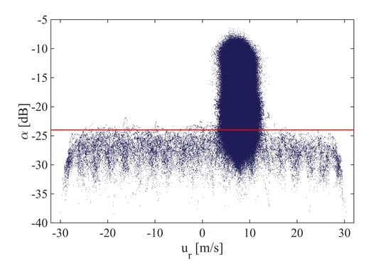
The CNR and SNR, , are quality indicators of the measurement and extend the data examination from only radial wind speed to two dimensions. Looking at individual measurement points in the radial-speed–carrier-to-noise-ratio diagram (–diagram) in Figure 1a, a correlation of CNR values and validity can be found. It can be seen that data points below the red line indicating a –24 dB level have high deviations in the range of –32 m/s to 32 m/s wind speed, thus, we assume that the points are invalid. The high scattering in this region may be caused by the LiDAR internal peak-fitting-algorithm of the frequency spectrum when there is no significant peak within the background noise. This results in a multimodal data distribution scattered around 0 m/s forming a comb shape. From this comb-shaped distribution the assumption arises that the peak-fitting-algorithm is not a homogenous process but is more attracted by certain frequencies, leading to a detectable accumulation at corresponding wind speeds.
While we assume that high data-density regions (HDDR) contain valid measurement points by the assumption of self-similarity and comparing means with the ultrasonic anemometer velocity measurements, here indicated by yellow and green regions in Figure 1b, we think that there is no indication based on the measurement distribution that data belonging to HDDR below a lower CNR limit, here −24 dB, is invalid (Figure 1a).
Main challenge of LiDAR data filters is the distinction of valid data from overlaid invalid scattered data. Outliers could have a real physical meaning, however, they may fall far away from the HDDR.
The threshold filter is commonly applied on CNR values of a data set. Data points beyond a certain range, will be filtered out. The low end edge, , indicates the level of signal gain where it is assumed that no information can be extracted anymore, while the upper edge, , filters out hard targets with high backscattering.
where represents CNR values of a valid measurement points. Depending on the manufacturer, the recommended and vary.
2.2. Static Standard Deviation Filter
One way of filtering wind speed data, when there is no secondary information such as signal quality or process quality indication, is the application of a standard deviation filter. Looking at the radial speed, all data with a higher scattering around the average radial speed, , than defined by a standard deviation depending tolerance will be filtered out.
where is the radial speed of a measurement point and is a multiplier of the standard deviation . In a data set, outliers can be eliminated with the right choice of . With the unsuspectingness of the measurement quality and existence of outliers, the -sigma interval may lead to a detectable data loss. The influence of different averaging times of is discussed in Section 4.
2.3. Iterative Standard Deviation Filter
The static standard deviation filter has low computational requirements; thus, it may be applied with multiple parametrisation at the same time. In contrast, the iterative standard deviation approach from Højstrup [19], adapted by Vickers & Mahrt [8] has higher computational costs due to a two looped application.
The standard deviation within a point-wise moving temporal interval is calculated. A measurement point is considered to be an outlier if the value exceeds the range of more than 3.5 standard deviations within the interval. The point is replaced by a linear interpolation. Outliers will not be replenished if four or more consecutive values are detected. This procedure is repeated until no outliers can be found. With each iteration the standard deviation factor will be increased by 0.1.
Appling both types of standard deviation filters imply the assumption of a Gaussian distributed filtering signal.
2.4. Interquartile-Range Filter
The interquartile filter or box plot filter descripted by Hoaglin et al. [20] is not based on a specific data distribution. For filtering, the interquartile-range (IQR) is calculated and will be subtracted to the first and added to the third quartiles. It is a threshold filter based on statistical dispersion. We used the following common parametrisation for valid measurement points :
where is the first quartile, is the third quartile and IQR is the interquartile range.
2.5. Combined Filter—Newman
A combined filter approach of LiDAR data can be found in the work of Newman et al. [16]. They applied a consecutive CNR-threshold filter and an iterative standard deviation filter described in Section 2.3 as quality control.
2.6. Combined Filter—Wang
As a second combined filter approach, we would like to mention the quality control of radial speed from Wang et al. [17]. In the original research, a CNR-threshold filter was applied to the data set before filtering with the interquartile-range filter from Section 2.4. As a third control body, all absolute radial wind speed differences smaller than two IQR of the deviations are marked as valid.
2.7. Dynamic Data Filtering
The main assumption of the newly proposed filter approach is based on the self-similarity of a measurement at a point in space. Assuming that the technical integrity of the measuring system is given and the measurement parameters are chosen well, we consider that repetitive measurements—stared or scanned—will not change their behaviour in an unpredictable way in a defined time interval.
In an idealised theoretical experiment without atmospheric and error influence a single point would appear in the diagram for a steady flow. Taking into account the distance dependency of adds vertical scattering, while temporal fluctuations of causes horizontal scattering. In reality individual measurements of and fluctuate around mean values, which depend on the chosen time interval. Valid measurement points are closer to these mean values, while outliers are characterised by a greater distance. This changes the density of the data distribution.
In general, it can be said that well parameterised measurements form valid HDDR, which may be overlaid by invalid data. In order to distinguish between those, the dynamic filtering approach is based on two subsequent process steps, temporal & spatial normalisation and data-density calculation. Two different implementations of the density calculation are presented and described in the following sub-sections.
2.7.1. Normalisation
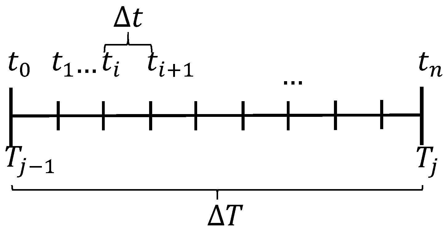
The intention of normalisation is to bring the measurement data to a relative frame of reference to reduce the absolute differences due to time and space. The effect is a compression of the data-density distribution. Considering the spatial and temporal dependency of the measurement values and we apply a corresponding normalisation. The definition of the normalisation time interval can be seen in Figure 2.
The overall filtering time interval is defined as – , whereas the normalisations interval is set as – . Thus, , and . For each measurement and , within one time interval and distance , we define the normalised values and :
and
The calculation of and is based on a one-dimensional Gaussian kernel, which may be expressed as
and
where is the amount of measurements within the time interval from to in the distance . The calculation of the bandwidth and follows the work of Botev [21]. Thus, each measurement value has been normalised individually based on their distance and time instant .
In the following, we consider individually normalised values and in the entire time period with , where is the amount of measurements point in the time interval .
The effect of normalisation can be seen by comparing Figure 3 and Figure 4. Both are based on the same dataset extracted from the measurement campaign descripted in Section 3.1 and represent an example of 30 min. Changes of wind speed within this time interval leads to a change of radial velocities, resulting in three HDDR located at different radial speed values (Figure 3). The distance dependency of the CNR causes an additional expansion of the data distribution on the -axis.
Applying the normalisation means switching the reference frame from to . This compensates spatial and temporal inhomogeneities and results in a denser data distribution where outliers can be identified with less effort.
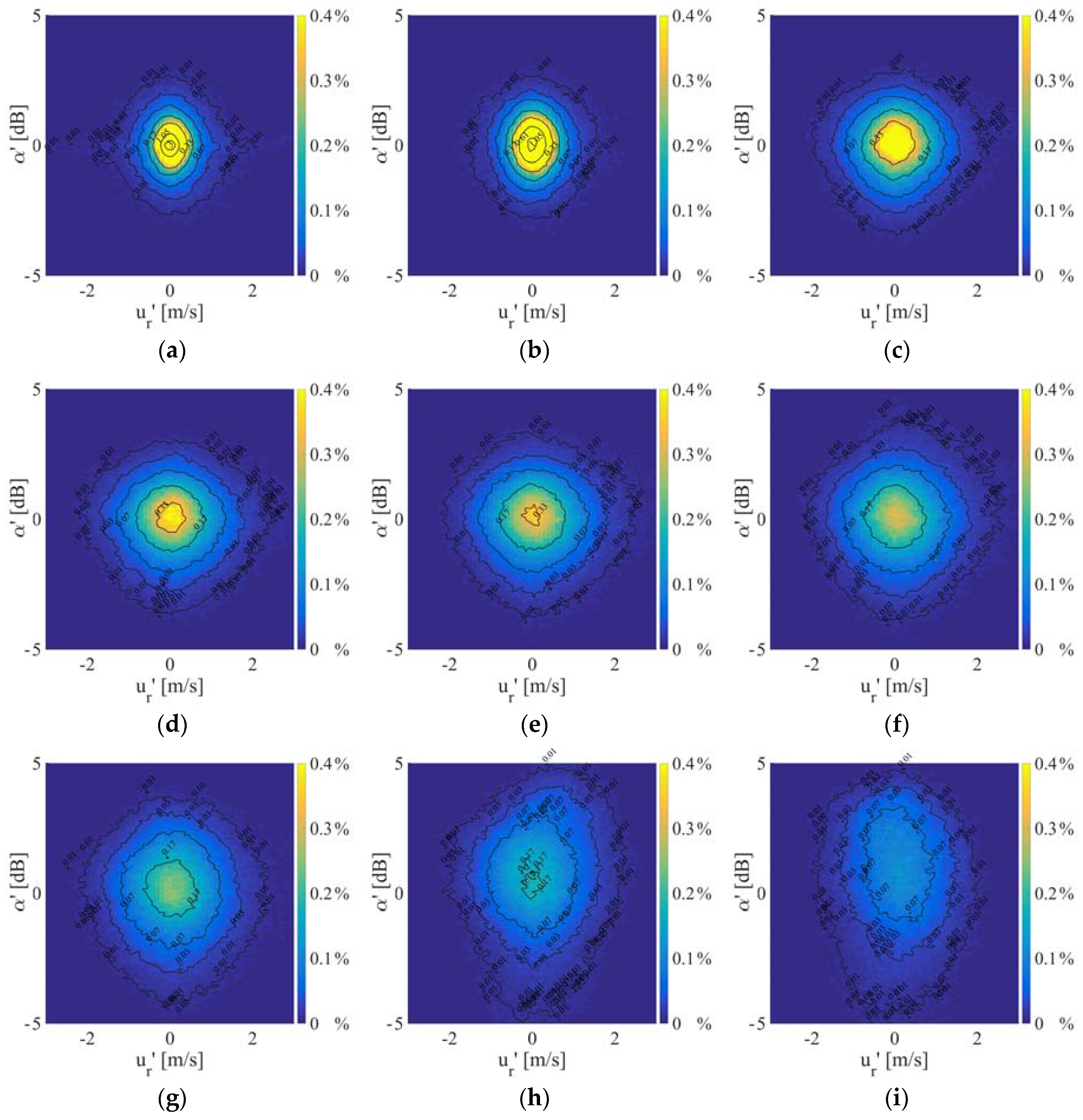
The influence of normalisation for different to the data density can be taken from Figure 4. In general, it can be said that the data-density distribution becomes softer and wider with increasing . For a better description of this behaviour, we fitted the resulting data density distributions with a bi-variate Gaussian function. We do not assume that the data density behaves in this way but we used the simplicity and reproducibility to characterise the change of parameterisation. The residual can be interpreted as the fitting quality. From Figure 5, it can be seen that the width of the bi-variate Gaussian function increases for and with increasing . The maximum value of the data density is subject to exponential decay.
The normalisation is independent of data-density calculation methods which will be presented in the following. The use of the data-density approach may as well be applied without prior normalisation.
2.7.2. Histogram-Based Data-Density
The first method to calculate the data-density is based on binning the normalised data in a 2D histogram. A suitable bin width for and is given by Scott [22] as
and
where is the standard deviation of , respectively is the standard deviation of , and is the amount of data points for time interval .
Scott assumes that the corresponding variable has to be normally distributed to use this parametrisation. Although it has not been proven conclusively that the wind speed is normally distributed, Morales et al. [23] have shown a great consistency of this theory for 10 min time intervals.
Instead of normalising the amount of data within a bin with the total number of data points, we normalise with the maximum bin count. Thereby the data distribution dynamically refers to the measurement and requires no absolute values.
The determination of validity is based on a correlation of data in the normalised reference frame . Calculating the contours for different densities, iso-lines form almost concentric circular shapes (Figure 4). Measurement points within the final contour will be marked as valid. To find the final contour that represents the separation line of valid and invalid data, we define an upper and lower threshold:
- The lower threshold value represents the lower percentage limit from which iso-lines will be calculated.
- The upper threshold can be seen as the reference shape that is based on the contour shape of the corresponding percentage density value.
By empirical testing, we found a correlation to determine the separation line. The easiest reproducible condition with the least computationally effort is presented in the following:
If the centre of a contour shape within the reference frame lies within the contour of the referenced shape corresponding to the upper threshold, all data points within this shape are marked as valid.
2.7.3. 2D-Gaussian Kernel Data-Density
The second method to determine the data density is based on the calculation of a two-dimensional kernel. We assume that and are subjected to random error processes; thus, their variability can be represented with a bi-variate Gaussian distribution [24], even when the overall behavior may be non-Gaussian. The validity ) for each measurement point with and in the time interval , with can then be assigned by the normalised data-density kernel in the reference system:
with
As the one-dimensional case from Section 2.7.1, the selection of is based on a Botev-estimator [21].
The distinction between valid and invalid data is now made by the calculation of the validity for each measurement point using Equation (11). The following classification is based on a threshold, which refers to the validity. Measurement point with a validity
may be seen as valid. The influence of to the resulting error is shown in the Appendix A.
3. Measurement Setups
The data for this study are drawn from three LiDAR measurement campaigns with different research objectives—an offshore campaign and two nacelle-based onshore campaign in the first half of 2015.
3.1. Offshore Ground-Based Comparative Measurement Campaign
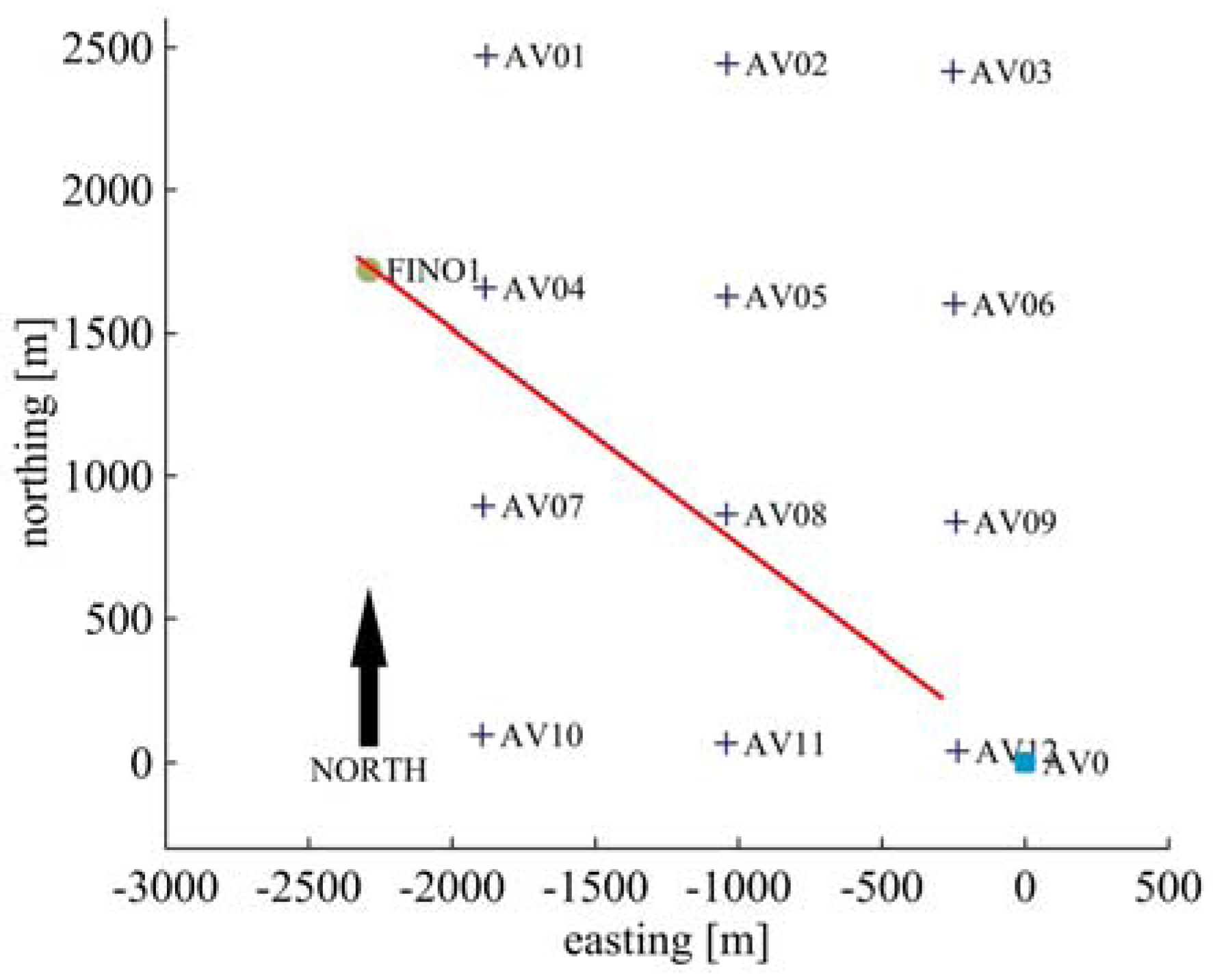
In the framework of the German research project “GW Wakes”, three scanning long-range Doppler LiDAR systems of type Leosphere Windcube WLS-200S [6] were operated in the offshore wind farm “alpha ventus” in the German North Sea. The wind farm comprises six 5 MW wind turbines Senvion 5 M with rotor diameter of = 126 m and hub height of = 92 m that are located in the northerly two rows and six 5 MW wind turbines Adwen AD5-116, formerly called M5000-116, with rotor diameter of = 116 m and hub height of = 90 m in the two southerly rows (Figure 6). The LiDAR used for the measurements was operated on the substation of the wind farm in the south east corner. “alpha ventus” is located close to the research platform FINO1 that is equipped with a meteorological mast [25]. In the following, all directions in the context of the offshore measurement campaign refer to the meteorological reference system, if not explicitly mentioned.
3.1.1. LiDAR Measurements
The used data was captured from 21.12.2013 15:35 h (UTC) till 19.01.2014 7:55 h (UTC). During this time period, the LiDAR was operated in a so called staring-mode with a fixed azimuth angle and a low elevation angle of = 0.2°, aiming at the ultrasonic anemometer at 41.5 m height at FINO1. The measurement frequency was set to with a pulse repetition frequency of 20 kHz, while capturing 82 equidistant range gates from 361 m to 2811 m with a range step of 30 m and 100 equidistant range gates from 2811 m to 2911 m with a 1 m range step. The pulse length was set to 200 ns or 59.96 m (FWHM).
Within the measurement duration of 28 days 16 h and 20 min, we were forced to interrupt the measurements for a total of 18 days 8 h and 30 min. The resulting comparable time intervals are comprised of 10 days 7 h and 50 min.
The positioning of the measurement near the anemometer on the FINO1 platform was ensured by an iterative hard-target method. First, we tracked the meteorological mast via horizontal PPI measurements (Plan-Position-Indicator scan) followed by vertical RHI measurements (Range-Height-Indicator scan) to identify the boom with the anemometer. We adjusted the final positioning of the measurement volume with the accuracy of the LiDAR system of 0.1° in azimuth and elevation. When the wind induced movements of the mast-boom-system are neglected, the maximum possible deviation of height of the anemometer and the centre of the range gate can be calculated as
The inclined measurement of 0.2° in combination with a pulse length of 59.96 m leaded to a negligible height difference within a range gate of 0.21 m. We verified the positioning of the LiDAR device by long term GPS measurements in combination with the geometrical dimensions of the substation. This resulted in an azimuthal orientation referred to the ultrasonic anemometer of = 306.47°.
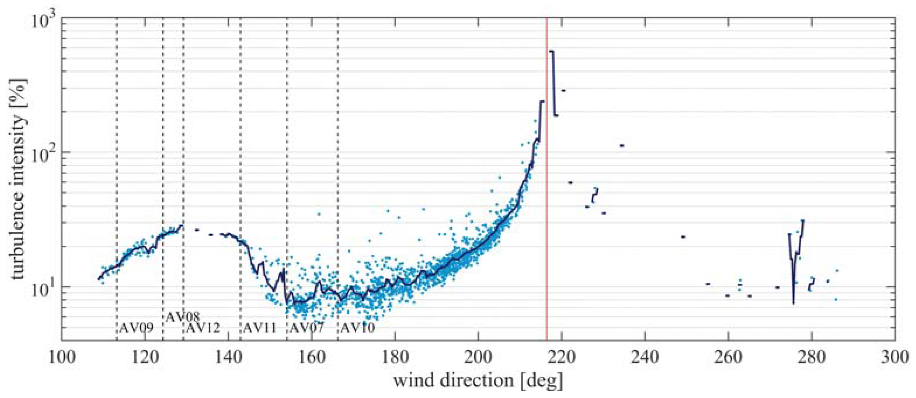
In this data set, wind directions have been measured at FINO1 within a range of 110° and 285°. Due to the fixed measuring geometry of the staring LiDAR, this could only measure the in-beam wind speed component. The result is a cosine relation between the wind speed in the wind direction frame of reference, , and the projected wind speed, (Equation (17)). For an incoming wind direction of 216.47°, the LiDAR measured perpendicular to the wind direction. Thus, the lateral wind speed component tends to become zero in average, which is why the turbulence intensity converges to infinity (Figure 7).
3.1.2. Ultrasonic Anemometer Measurements
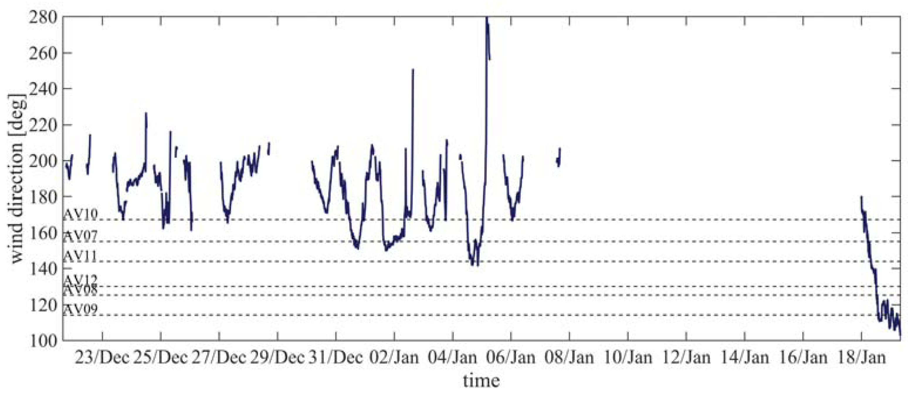
The 3D ultrasonic anemometer used for the comparison with the LiDAR data is a Gill R3-50 mounted at the meteorological mast FINO1 at the height of = 41.5 m on a 6.5 m long boom orientated at 308°. Vertical wind speed, horizontal wind speed, wind direction and air temperature data have been recorded with a sampling frequency of . The original wind direction measurements have been corrected on the basis of the approach of Schmidt et al. [26] by using staring LiDAR measurement to determine misalignments. The correction of Schmidt et al. includes the previous correction of the mast influence performed by Westerhellweg et al. [27]. Figure 8 shows the frequency of the wind speed and wind direction distribution within the time period. The temporal change of the wind speed and wind direction can be seen in Figure 9. Horizontal lines within Figure 9 indicate a possible wake shading of the named turbines for that particular wind direction. Due to simplicity, these wind directions have been calculated on the basis of geometric correlations, and we neglect wake expansion and meandering effects.
3.1.3. Onshore Nacelle-Based Wake Measurements
The second and third data set were acquired within the German project “CompactWind”, in which two of the previously described LiDAR devices have been installed on the nacelle of an eno114 3.5 MW wind turbine with a rotor diameter = 114.9 m and a hub height of = 92 m. The onshore wind farm consists of two wind turbines from the same type and is located near Rostock in the village Brusow. The surrounding terrain is slightly hilly with a compact forest to the east.
The first measurements were performed from 14.05.2015 02:30 h (UTC) till 14.05.2015 06:00 h (UTC). Here, we show only one LiDAR in measuring horizontal PPI scans with 0°elevation at nearly hub height with a total azimuthal opening angle of 40° centred in downstream direction. Each of the 571 scans took 20 s, resulting in a repetition period of 22 s, including an initialisation time. We parameterised the Leosphere Windcube 200s with a pulse length of 200 ns respectively 59.96 m (FWHM) and an accumulation time of 200 ms with a pulse repetition frequency of 20 kHz. In this time period in which the turbine was operating a significant wake was measureable. Within the framework of “CompactWind”, we were able to alternate the nacelle mounted LiDAR from the described Leosphere device with a Stream Line XR LiDAR by Halo Photonics. The here used Stream Line XR dataset is shown as an example of general applicability of the dynamic data filtering approach.
The corresponding third data was captured from 31.10.2016 00:00 h (UTC) till 31.10.2016 00:30 h (UTC). In that time period, the LiDAR was operating in PPI mode using the above mentioned opening angle, accumulation time and scan speed. The measurement was parameterised with a pulse length of 100 ns or 29.98 m and a pulse repetition frequency of 10 kHz.
4. Results
For the validation and comparison of the new proposed dynamic filtering approach in Section 2.3, we applied all described filters on the data of the three measurement campaigns from Section 3. The influence of filtering on the data availability and the velocity error regarding the ultrasonic anemometer from the offshore campaign are shown in the following. Moreover, the behaviour of the velocity error will be discussed.
4.1. Evaluation of Filtering Based on Staring Measurements
For the error calculation of ultrasonic anemometer data and the LiDAR data, the initial question arises how different measurement concepts can be mutually compared. The metric used to validate the new and other filters is based on average velocities. We present also results for the velocity standard deviation for sake of completeness. However, we consider that the data available is not adequate for drawing conclusions in our ability to derive turbulence properties. Although both devices measure within a certain volume—in an idealised case, the same volume—this differ in spatial dimensions. While we estimate the ultrasonic measurement volume from technical drawings as a cylinder with , the corresponding equivalent volume for the LiDAR laser beam of the Leosphere device in the here used configuration is approximately . By this, the LiDAR measurements use around 22 times the ultrasonic anemometer volume. If we consider that the individual ultrasonic transmitter and receiver heads measures on the surface shell of this cylinder, the ratio is in the magnitude from 10 to 100. The effect of spatial averaging of LiDAR measurements on the variance of the line-of-sight measurements and the associated challenge of deriving turbulent properties, in a substantial scientific manner, from LiDAR measurements is discussed in a plurality of publications. First, LiDARs filter out high frequencies depending on the effective sampled volume. This distorts the velocity variance. Moreover, Sathe and Mann [28] show that atmospheric conditions play an important role affecting the ability to measure turbulence. Sathe and Mann [28] published an extensive review of turbulence measurements since the beginning of LiDAR based remote sensing in which they highlight that the variance is very dependent on atmospheric conditions. We conclude from the work of Frehlich [9] and Sathe and Mann [28] that an adequately determination of the wind speed variance is possible, with a comprehensive approach including raw LiDAR data. Such treatment was out of the scope of this work, wherefore we focused in the following inter-comparison of the LiDAR filter on the average wind speed.
To minimise the different volume averaging effects and to comply with other comparisons of LiDAR measurements and met mast anemometers [29,30,31,32,33], we applied filtering in clustered temporal segments of 10 min. We have deliberately refrained a data availability pre-filtering for the calculation of the 10 min average velocity and velocity standard deviation. This is intended to create a greater transparency to the overall filter behaviour.
We evaluated the effect of variable averaging times for all filters with a smaller data set from the already presented campaign. The impact on the total error in combination with the normalisation time for the dynamic data filters can be seen in the Appendix B. We conclude from Figure A1, Figure A2 and Figure A3 that the results of the dynamic data filters vary depending on the used parametrisation. The parameters should be adjusted with respect to the purpose of data analysis and the desired error calculation, as can be seen in Figure A3. For a better readability, we opted for one parameterisation each. The selection of the validity value regarding the error behaviour in Appendix A was chosen as a compromise between the average error and the root-mean-square error (RMSE) of each, velocity and velocity standard deviation. The histogram-based dynamic filter has been used with a lower filter threshold of 0.02% and an upper filter threshold of 0.29%, through the Gaussian kernel based implementation was set to a validity level of 16.94%.
In total 4325 10 min time intervals have been processed for the following results. The standard deviation filter was used in a two-sigma configuration and the CNR-threshold filter, as well used in the combined filter approaches, in a parametrisation of and . To the best of our knowledge, we were also porting the filter approach by Wang et al. [17] for the first time to staring mode and horizontally scanned LiDAR data. So far, this filter approach has been applied only for VAD measurements. Further, we tested the proposed quality control from Newman et al. with Leosphere Windcube 200s data for distances beyond those in the original publication [16].
4.1.1. Data Availability
We define the here titled data availability as the ratio of the amount of data for one point in space of the filtered to the unfiltered LiDAR data within a time interval:
Only 10 min time intervals were considered that amounts to the theoretically number of measurement points. A data availability of 100% within a time interval implies that all measurement points are marked as valid. To calculate the data availability, a spatial based comparison (Figure 10) for all ranges and the corresponding closest volume to the ultrasonic anemometer has been made and was summarised in Table 1. For the data availability calculation we considered only in non-overlapping time intervals of 10 min.
While all filters show a consistent mean result above 75% data availability, the behaviour with respect to the range is dependent on the type of filter. All filters using the CNR-threshold approach show the same decay in availability related to the distance dependency of . With the decrease of the CNR over the distance, temporal fluctuations of are partially filtered out if they exceed the CNR-threshold. By this, the data availability decreases continuously. We assume that the here shown behaviour of all CNR-threshold containing filters is similar to the theoretical and empirically stated data availability decay with increasing distance described by Boquet [34].
It appears that the combined filter by Newman et al. [16] does not produce any visible deviation from the CNR-threshold filter even when they applied an addition iterative standard deviation filter that, when applied alone, provides an availability of 98.5%. It seems that as well the filter approach by Wang et al. [17] leads to a higher data availability compared to a sequential calculation from the individual availabilities. The output of the two-sigma standard deviation filter exhibits an overall availability of over 95% for the entire distance and increases slightly with more distant range gates. Because it is based on the deviation around the average of wind speed, this behaviour can be explained with the geometric correlation of the measurement setup. From a distance of approximately 2100 m, the laser beam measured outside the wind farm where the flow was not affected by wind turbine wakes. In contrast, the data availability of the iterative standard deviation filter decreases by 1% over distance. It is shown that the interquartile-range filter produces a smaller availability of 94% compared to 99.3% in theory for normal distributions. This may be an indication that the data distribution within the 10 min intervals does not exactly follow a normal distribution.
If we neglect all filters that do not take into account the distance dependency of , we can compare all CNR-based filter with the dynamic data filters. It can be seen that the histogram-based filter results in a nearly constant data availability of 90%. The kernel-based dynamic data filter shows a drop of data availability in closer distances followed by a constant slight decrease over the distance. From this behaviour it cannot be confirmed that the data availability of the dynamic data filters follow the decay stated by Boquet [34]. We assume that the main reason for this is based on the temporal and spatial normalisation of the LiDAR data. By normalising with the most probable value within the normalisation interval, measurement points close to , which would exceed the CNR-threshold, are marked as valid and contribute to high data availability.
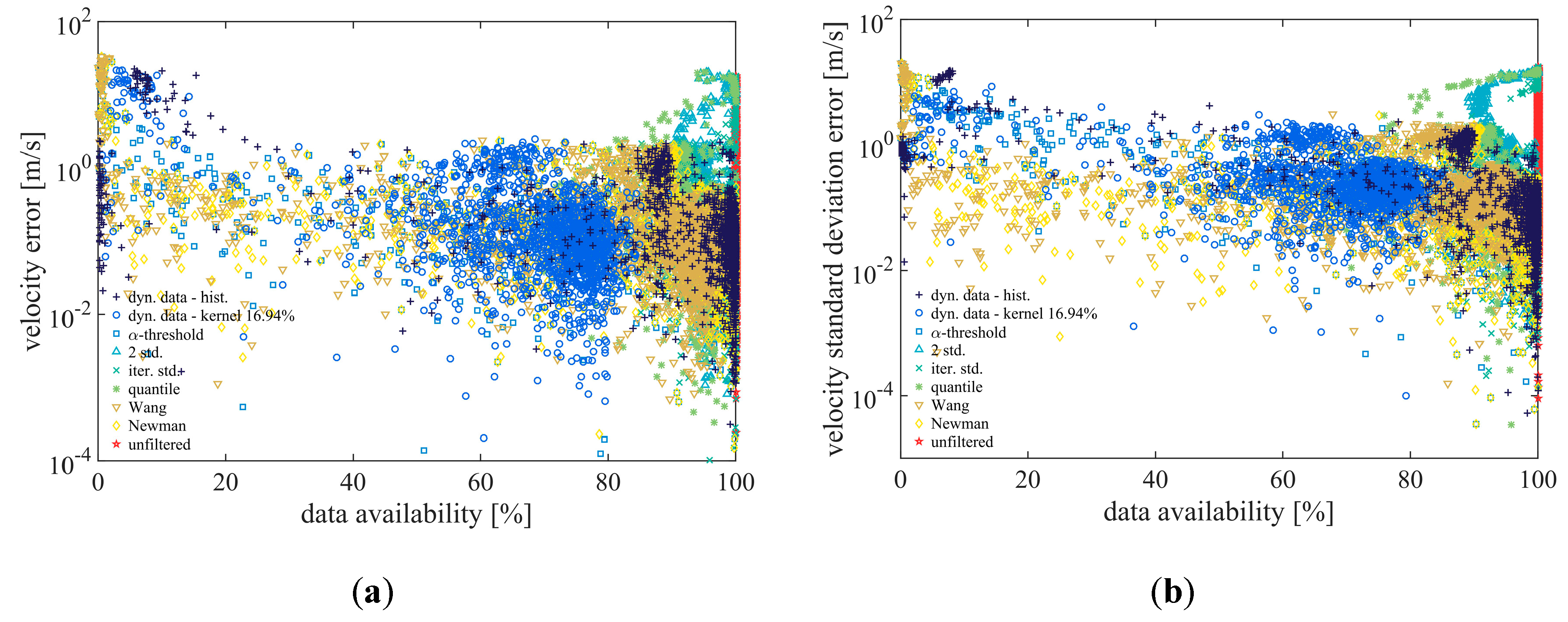
Figure 11 shows the error distribution of the velocity and the velocity standard deviation in dependency of the data availability on the basis of 10 min means. A high correlation of the general appearance of Figure 11a,b suggests a causal connection of the velocity and the velocity standard deviation error. While both standard deviation filters and the interquartile range filter mainly show error values above 80% data availability, the data distributions of the dynamic data filter and CNR-threshold based filters are widely scattered. We see a repeating pattern of data point clusters in Figure 11a,b that appears to be individually scaled for each of the dynamic and the combined filters.
Although both dynamic data filters use the same normalised dataset, the observed differences in data availability appear for unknown reason. In this test case, the full potential of conservation of data availability by the kernel-based dynamic data filter cannot be seen. We assume that based on the behaviour shown (Figure 10), the data availability of the CNR-threshold based filters will drop significantly faster with increasing distances than of the dynamic data filters.
4.1.2. Comparison of LiDAR and Anemometer Velocity Measurements
In the following section, we quantify the accuracy of all filtering methods. For this we assess the discrepancy of estimated velocities taking into account filtered, unfiltered data and the reference data of the ultrasonic anemometers. We distinguish between the average error, which is defined as the arithmetic mean, and the RMSE. As we mentioned previously the assumption of LiDAR data behaviour is included in every filter. The resulting errors of the following comparison can be seen as a measure of correctness of this filter included LiDAR data behaviour.
Because the fixed LiDAR measurements can strictly measure the in-beam directed wind vector, the ultrasonic anemometer data has been projected to the LiDAR measurement geometry. The original anemometer velocity information has been adjusted on the basis on the study of Westerhellweg [26] to compensate the mast wake. Due to the marginal changes of the wind speed magnitude of the low elevation measurement of the LiDAR of = 0.2°
we used the filtered radial line-of-sight velocities of the LiDAR without additional projection to the horizontal plane. By this assumption, the projection of the ultrasonic anemometer is reduced to a single rotation around the z-axis. The index refers to the LiDAR reference frame, whereas index stands for the meteorological reference frame.
where −53.53° is the directional offset of the LiDAR reference frame and the meteorological reference frame. In advance, we carried out correlations of wind speed time series of each range gate with the ultrasonic anemometer time series to find the closest measurement range gate.
The direct comparison of wind speed and the calculation of deviations of the filter associated time series show that all filters behave in a similar manner for the greater part (Figure 12a,b). The CNR threshold and both standard deviation filter did not select all outliers as accurate as the dynamic data and combined filter approaches. High average velocity errors seem to correlate with recognisable peaks in the velocity standard deviation curve (Figure 12a,b), which is an indicator of high scattering in the filtered data. This may occur when the invalid data from the “comb”-shaped data distribution (Figure 1) is classified as valid.
The velocity error and the velocity standard deviation error over the wind direction show high values for several inflow directions (Figure 12c,d). Based on the turbulence intensity distribution from Figure 9 and the standard deviation error from Figure 12d, it cannot be differentiated whether the visible increase between 110–145° is due to the mast shadow or by the wake of the turbines AV09, AV08, AV12 and AV11. Indicated by peaks of the average velocity error (Figure 12c) close to the theoretical turbine directions we could conclude that these arise by wake shading. Meandering effects, wake-induction-zone interaction, turbine and wind farm circulation could not be taken into account; thus, differences in the turbine positions and the corresponding peaks may occur. The smallest increases can be determined for AV09 in a distance of 2230 m and AV11 (2069 m), whereas significant peaks may be caused by AV10 (1669 m), AV08 (1512 m) and AV07 (916 m). Because AV08 and AV12 are close to each other, we cannot differentiate individual proportion of the wakes to the error.
It is surprising that the average error in the mast wake (<145°) is less for unfiltered LiDAR data than for processed ones. This could be indicating that the filters sort out physical reasonable values. While all filters have increased errors in determining the correct velocity standard deviation, the two-sigma standard deviation filter produced noticeably low values in this region. The increase of the errors for this inflow range may be explained due to different measuring volumes. While the anemometer is exposed to increased fluctuation directly in the mast wake, the LiDAR measures a mixed velocity of free and affected flow within the elongated volume. It can further be seen from Figure 12c,d that the LiDAR is not capable of capturing perpendicular wind speed components (216° inflow direction) in a good manner. According to the errors shown in Figure 12c,d an undisturbed inflow occurred from 180° to 210° and from 220° to 265°.
In Figure 13a,b linear correlation of the ultrasonic anemometer data and the LiDAR data has been done for the velocity and the standard deviation. Here, all data are presented without a containment of wind direction. Therefore, these results include situations where the ultrasonic anemometer, as well the LiDAR measurement is in free flow, in wake flow of the mast and in the wake of the wind farm. We observe regression slopes in the range from 0.866 to 0.974 and regression coefficients from 0.78 to 0.9. These relatively low coefficients are driven by outliers, which are not very frequent, but have a large deviation. These wrong data points evidence in our opinion the discrepancy between point and volumetric flow interrogation in complex flows. In effect, these large deviations occur for data in the mast wake predominantly. In the study of Schmidt et al. [26] a subset of these data, specifically restricted to free flow, showed a very high correlation. These results are confirmed here as shown in Table A2. Since this is mainly a physical effect, it is impossible for any of the filters to reduce the error. It is to be noted that the large deviations concentrate in a certain wind speed range. This is due to the wind conditions during the measurement period, where wind speeds above 6 m/s were found very often for wind directions where the ultrasonic anemometer was shaded by the mast, whereas lower velocities occurred in free flow conditions.
While the velocities correlate quite well, the regression of the standard deviation is widely spread for the different filters. All linear regression parameters are reported in Table 2. In combination with Figure 13a,b, Figure 13c,d extend the linear regressions with an uncertainty interval equal to the RMSE. For better visibility, we omit these ranges in Figure 13a,b, and plotted them separately in Figure 13c,d. It can be recognized that ultrasonic anemometer data in a wide range around 10 m/s is associated with high deviations of LiDAR velocities (Figure 13a). A corresponding behaviour is also present in Figure 13c. Even Figure 13c,d give the RMSE for specific velocities respectively velocity standard deviations a conclusion about the overall performance needs to consider the error frequencies in Figure 14.
In general, it can be said that the application of the combined and dynamic filter approaches leads to smaller errors of the velocity and velocity standard deviation compared to other filters. With the exception of the combined filter approach from Wang et al. [17] that was able to reduce the average velocity standard deviation error to 0.0 m/s, both dynamic data filters generated the smallest error in the comparison of three out of four error calculation categories. To give an overview of the overall performance, we distinguish between all wind directions in Table 1, wake affected situations, 110–180° wind direction, and free inflow, 180–210° wind direction, in Table A1 and Table A2 in the Appendix C. In each of those data classifications, we see mostly a similar behaviour of the filters in mutual perspective as well in relation to the results in Table 1.
4.1.3. Error Analysis
In order to gain a better understanding of the error behaviour and insight into the resulting error, we performed an error analysis. For this, the frequency distribution of the errors is calculated.
Figure 14 illustrates histograms for the RMSE of the mean velocity and the velocity standard deviation of all 4325 10 min intervals with a non-constant bin width increasing exponentially. It can be seen that the errors are subject to a double log-normal distribution or Pareto distribution. Explaining the cause of this specific distribution is out of the scope of this paper. Nevertheless, we do a qualitative analysis supported by the cumulative distribution presented in Figure 15. While the distribution of absolute average velocity error of the unfiltered LiDAR data (red line) follows this behaviour very well, local deviations of all used filters can be found from a value on of approximately 3 m/s (Figure 14a). The error distribution of the Gaussian kernel dynamic data filter seems to be displaced towards higher errors. We fitted a double logarithm distribution to the histogram to determine the most probable error of the fitted distribution which is provided in Table 3.
The error behaviour of the standard deviation shows double peaks at 0.1 m/s and 4.4 m/s for the unfiltered case and suggests that two functions overlap here. The frequencies of the velocity standard deviation error, for the filtered data, show as well a second peak shifted to ca. 1 m/s. These error behaviours are also confirmed by Figure 15a,b that shows the resulting errors for error values below a certain threshold (x-axis). It turns out that Figure 15 is equivalent to the cumulative distribution of error from Figure 14. While the resulting RMSEs increase up to 3 m/s error threshold for all filters, this is a turning point followed by a split in behaviour. As expected, the unfiltered LiDAR data results in the highest error up to a threshold of 17 m/s. This error is exceeded from the combined filter approach of Newman et al. [16] and the CNR-threshold filter respectively the combined filter of Wang et al. [17] at the error thresholds of 26 m/s and 29 m/s. While the average error of those three filters are below the unfiltered data, it turns out that the RMSE, as a measure of velocity dynamic accuracy, are the highest with in the test case shown in Table 1. A possible explanation may be that all three filters are based on the CNR-threshold filter. While these three filters produce the smallest error up to a threshold of 13 m/s, an enormously increase is followed till the maximum error is reached.
The maximum error can be determined by following the error threshold to the maximum value. By comparing the error behaviour from Figure 15a,b with the theoretical accumulated function of a Pareto distribution (root function), the assumption of multiple overlapping distributions may be confirmed. We see the typical increase of a root function several times in Figure 15a,b. E.g., the behaviour of the histogram based dynamic data filter standard deviation curve in Figure 14b shows a root functional increase from 0 m/s to 10 m/s and again from 10 m/s to the maximum error. This hypothesis is supported by the second peak of the same graph in Figure 14b around about 10 m/s. Similar behaviour can be seen for the remaining filters in Figure 14b and Figure 15b.
4.2. Evaluation Based on Scanning Measurements
The goodness of the filters must be evaluated in a broad range of applications. The previous staring study does not include the additional spatial effect given in scanning trajectories. Such validation work, is, however, limited by a missing reference. In effect, it is very costly to setup an experiment to validate a scanning LiDAR at least at some points within the trajectory. Therefore, such evaluations have to be done here only at the qualitative level. In this respect, we processed the nacelle-based PPI-scanned measurements analogous to the staring mode measurement data, with the exception of the application of the standard deviation filter and the spatial normalisation within the dynamic data filter. Due to lower spatial measurement frequency of compared to the staring mode measurements of we enlarged the selection of radial wind speed data in beam-wise and azimuthal direction to form an equivalent amount of data to calculate the standard deviation within a 10 min segment. All CNR-threshold based filters have been used with a parametrisation of and . The normalisation of CNR and radial speed for PPI-measurements has been extended by calculating the temporal and spatial averages for azimuthal bins of 1°. Thus, we expect to consider different characteristics of the wake regions and allow potential different backscattering properties due to the complex flow structure. All other filters were used as described in the referenced publications and were applied thereon range- and angle-wise.
Next, we filtered the PPI scans in 10 min segments and interpolated them scan-wise to a regular Cartesian grid. We averaged the individual scans afterwards to 10 min means.
In the visualisation of the unfiltered data, it can be seen that high CNR-structures (Figure 16r) correlate with structures in the wind speed (Figure 16p) and its standard deviation (Figure 16q). The probability of occurrence of those structures in a 10 min average is improbable. It is unphysical in the sense of a flow field that sharp, irregular structures emerge in the beam direction (Figure 16r). Therefore, we assume that these structures occur due to invalid measurements. However, to produce an interference-free data set, we tried to exclude those by filtering.
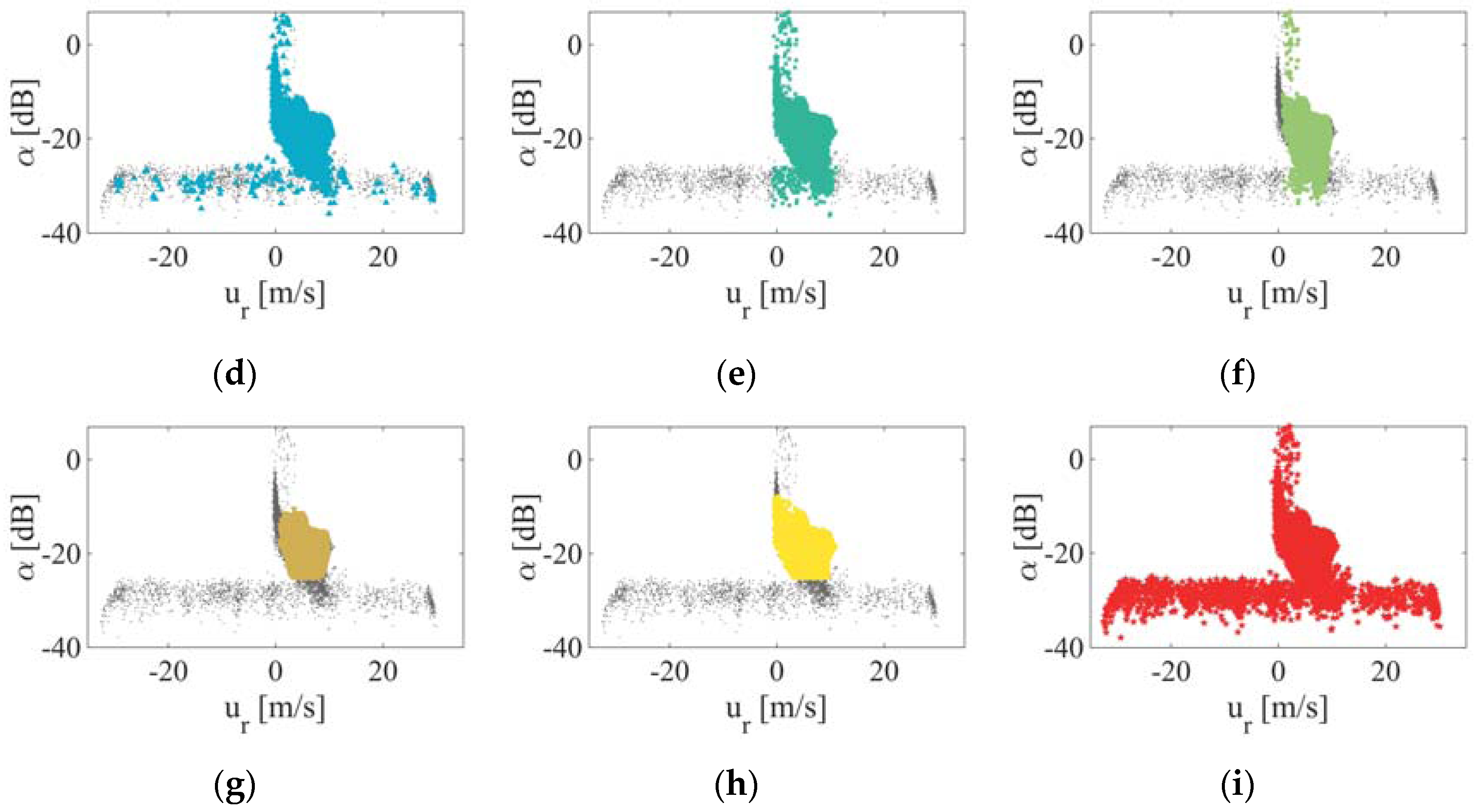
We may explain those structures regarding the diagram and the functioning of the individual filters (Figure 17). The data accumulation of measurements points close to 0 m/s in a wide range of may appear due to partly shading of hard targets or unknown reason. Obstacles, such as meteorological masts, overhead transmission lines or rotor blades of other turbines influence the laser beam partly, complete or multiple times and affect the backscattering. Therefore, a second distinct peak, besides the one of the wind speed appears in the frequency spectrum. Thus, obstacles causing high-backscattering high-amplitude peaks are fitted as often as the wind speed peaks. Figure 17 gives an indication of the functioning of the different filters. It can be seen that only the dynamic data filters and the combined filter approach by Wang et al. [17] managed to eliminate the high scattering of in the “comb”-shaped data distribution and prior described the data accumulation close to 0 m/s.
Regarding Figure 16 and Figure 17, a relation between the mentioned exposed structures and the filtering can be made. Based on this test case of scanned data, we observed that dynamic data filters are capable to identify more outliers than the other filters.
As a proof that the dynamic data filtering approach is not system specific, we present an example of PPI data from the second part of the nacelle-based measurement campaign from Section 3.1.2 captured with a Stream Line XR. In the following, we will illustrate the data-density distribution in the diagram and the normalised LiDAR data in the reference frame as a proof of similar data behaviour in comparison to the Leosphere LiDAR.
As can be derived from Figure 18a, the overall data density of the Stream Line XR dataset shows similar behaviour in comparison to the Leosphere Windcube 200s LiDAR data in Figure 3. A horizontal scattering in the radial velocity in combination with a vertical scattering of the CNR is shown in both visualisations. The application of the temporal and spatial normalisation from Section 2.7.1 results in a comparable data density distribution.
It is noticeable that the density distribution of the normalised LiDAR data of the Stream Line XR device tend to form a pyramid distribution (Figure 17b), whereas the density shown in Figure 4 resembles a bi-variate Gaussian distribution. The normalisation provided here was applied with a = 60 s and may therefore be compared with Figure 4f. From similar behaviour of forming a dense data distribution in the reference frame, we confirm the suitability of the possibility of application of the dynamic data filter as presented in this paper.
5. Conclusions
We introduced a new approach to filter line-of-sight long-range Doppler LiDAR data dynamically. This considers the influences of atmospheric conditions, device dependencies and the measurement setup. The new methods take into account the radial velocity and the signal quality in a bi-variate manner based upon the assumption of self-similarity of valid data. Here we performed a benchmark of two implementations of the new dynamic filtering approach together with five state-of-the-art filter methods used in research and industry applications. First, a temporal high resolved time series of approximately 1.5 weeks measured in a distance of 2864 m by a minimal inclined long-range LiDAR was compared against an ultrasonic anemometer with means of 10 min to make a quantitative evaluation. Second, we performed a qualitative analysis to infer filter performance for cases of scanning interrogation of the wind field. Within this study the combined research filter approaches by Newman et al. and Wang et al. have been ported to a Leosphere Windcube 200s dataset.
This study demonstrates, that the common practice of using fixed CNR-threshold based filters may lead to unnecessarily reduced data availability. This limitation can be overcome by more elaborated methods, which implementation is technically feasible with low computational cost. We were conditionally able to decouple the commonly associated distance dependent data availability on the CNR by introducing a temporal and spatial normalisation of measurement properties within the dynamic data filter approach that are also capable of complex changing flow situations and variations of the CNR over time. However, their general application must be thoroughly studied. Regarding the mean velocity errors, it is shown that high data availabilities do not necessarily lead to good accuracies and lower data availabilities not imply poor agreement with the reference.
The resulting errors of this test case are in the range from 0.30 m/s to 0.76 m/s for the average velocity, from 2.1 m/s to 3.1 m/s for the RMS velocity error, from 0.00 m/s to 2.17 m/s for the standard deviation error and from 0.9 m/s to 4.1 m/s for the RMS velocity standard deviation error.
The overall results of all filters and the parametrisation study of the Gaussian kernel based dynamic data filter indicates, that filtering can be done with the focus on the velocity dynamics in terms of the standard deviation or the average velocity. Moreover, the error evaluation varies whether the average error or the RMSE is considered. In comparison to all filters, both implementations of the new approach produce the smallest error in three of four error calculation categories whereas the combined filter approach by Wang et al. was able to diminish the standard deviation velocity error to 0.0 m/s.
Depending on the discipline, the application of wind LiDAR filters and the magnitude of commonly accepted errors vary, wherefore the here shown differences in the results should not be underestimated. Even small differences in the average wind speed can be the decisive argument in the resource assessment with respect to the realisation of a wind park. It is up to each user to balance the computational effort with the needed accuracy. The selection of a filter should comply with the analysis requirements. While the commonly used fixed CNR-threshold filter is used for fast and robust results, the histogram based dynamic data filter can be used to increase the data availability while maintaining a high accuracy. Critical applications in which a certain maximum error may not be exceeded require a more stringent filter than applications where the frequency of certain errors is a relevant criterion. The conducted error analysis has shown that the frequency distributions of errors do not show a normal distribution and are very distinct from each other.
In the valuation of filtering results of scanned measurements in full-scale experiments with two different LiDAR devices, it was shown on basis of temporal means that certain error structures in the flow field and the CNR-mapping were filtered by Wang et al. and the dynamic data filter approach in a good manner.
Due to the behaviour of the dynamic data filter approach within the here presented test cases, we conclude the assumption of self-similarity to identify valid data points as very reasonable. An accompanying limitation within this approach is the need of a certain amount of valid data to form dense clusters for the calculation of the data density. At the same time, this limitation can be seen as an advantage, since large quantities of data can be processed at once and thereby the proportion of valid data can be increased. Because of the applicability of scanned as well as stared measurement setups we see the dynamic filter approach as a promising tool for different types of LiDAR measurement setups. The results shown here are a further step in the development of filter techniques for explicit LiDAR applications and prove that self-similarity can be used as a criterion for LiDAR data filtering. Regarding the reproducibility of the comparison results, further investigations of the behaviour and limitations of this approach should be performed with a plurality of different measurement situations that could not be part of this study.
Acknowledgements
We thank eno energy systems GmbH and the RAVE (Research at alpha ventus) consortium for the support during the measurement campaigns. We are also grateful to the reviewers and Juan José Trujillo, Andreas Rott, Marijn Floris van Dooren, Laura Valldecabres Sanmartin and Wilm Friedrichs at the University of Oldenburg for the valueable discussions. The presented work has been funded by the Federal German Ministry for Economic Affairs and Energy of Germany (BMWi) in the framework of projects CompactWind (contract No. 0325492B) and GW Wakes (contract No. 0325397A).
Author Contributions
Hauke Beck wrote this paper and conducted related research. Intensive reviews were done by Martin Kühn.
Conflicts of Interest
The authors declare no conflict of interest.
Abbreviations
The following abbreviations are used in this manuscript:
| LiDAR | Light detection and ranging |
| ABL | Atmospheric boundary layer |
| LOS | Line-of-sight velocity |
| CNR | Carrier-to-noise-ratio |
| SNR | Signal-to-noise-ratio |
| HDDR | High data-density region |
| PPI | Plan-Position-Indicator |
| RHI | Range-Height-Indicator |
| PRF | Pulse Repetition Frequency |
| FWHM | Full Width at Half Maximum |
| RMS | Root-mean-square |
| Avg | Average |
| Std | Standard deviation |
| Abs | Absolute |
Appendix A. Infuence of the Normalization Time on the Validity
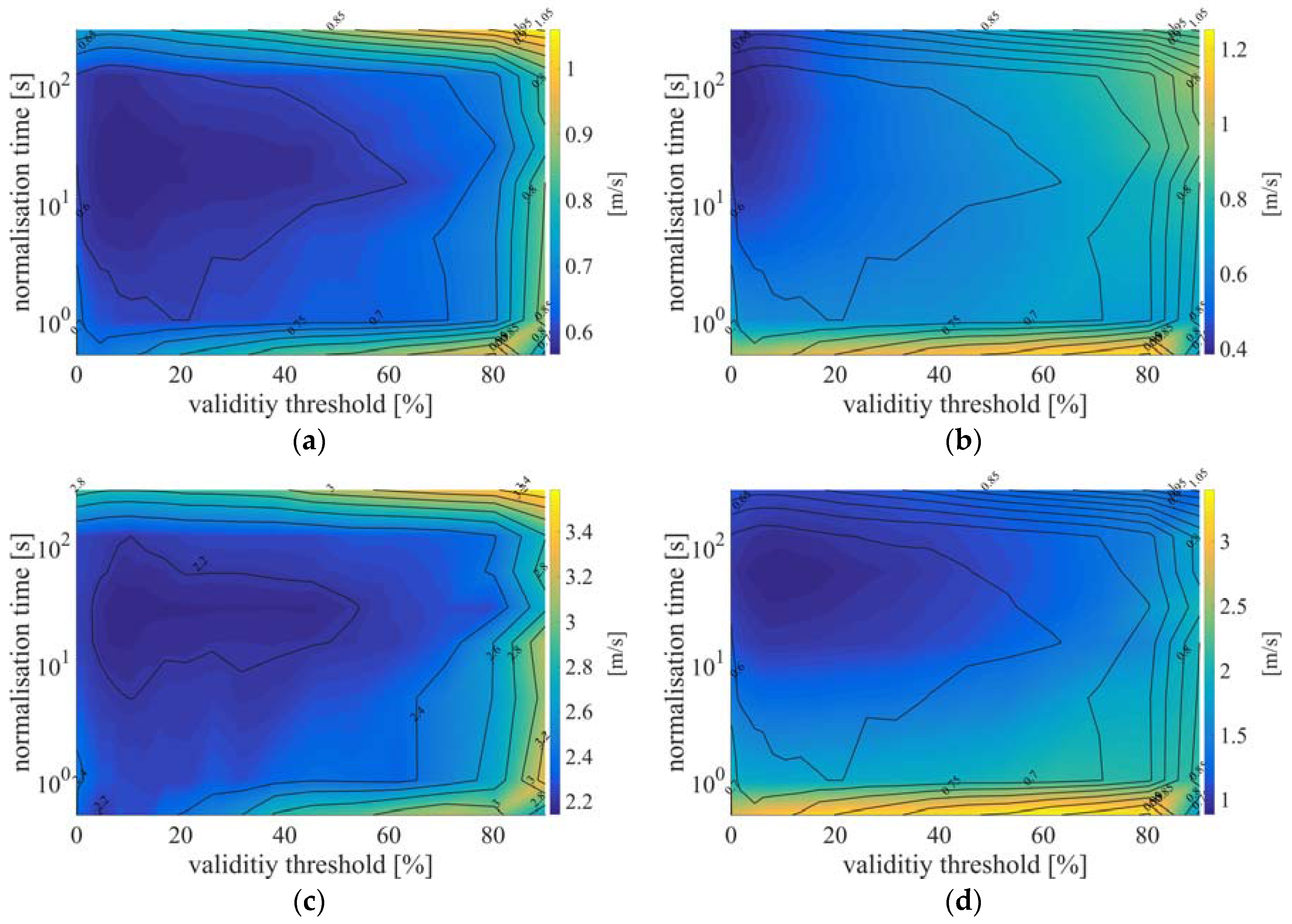
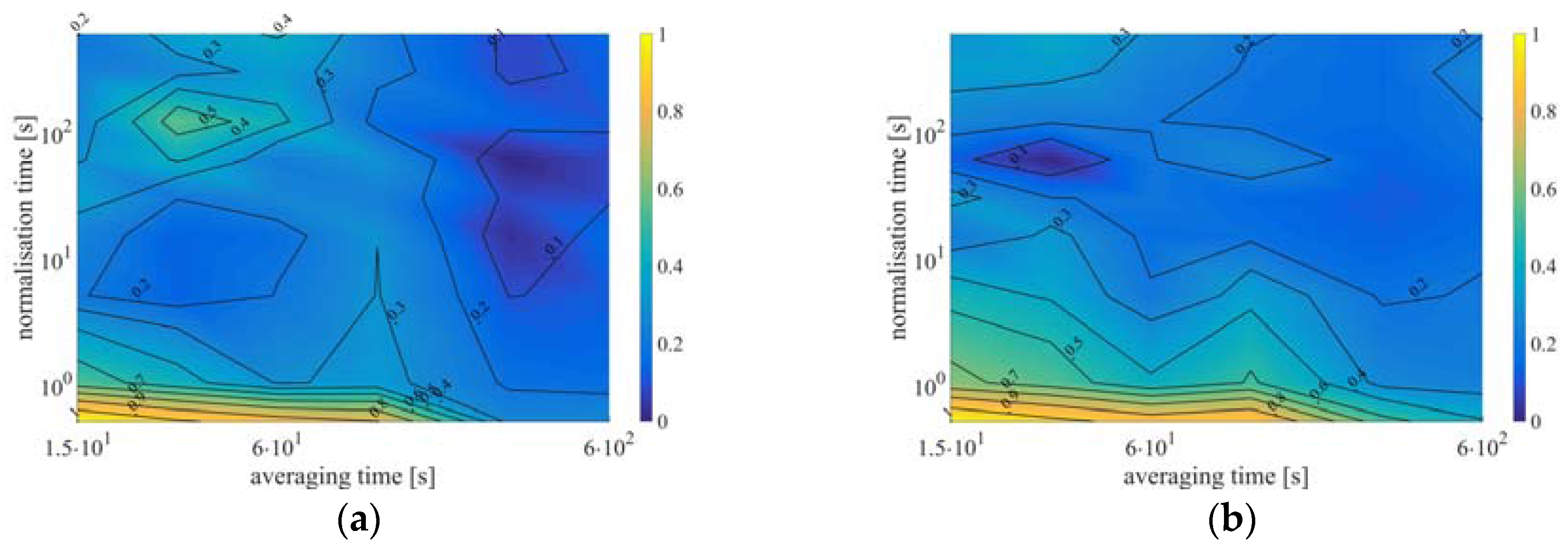
The discretisation of the main averaging interval in different normalisation intervals changes the data density as shown in Section 2.7.1. The calculation of the Gaussian kernel based on different data densities influences the choice of a suitable validity value . Based on the entire data set from Section 3.1.1, we performed a parameter study that considered the resulting average errors and the RMS of velocity and velocity standard deviation. For this purpose, we used different combinations of , in a range from 0.5 s to 300 s used and validity values from 10% to 100% for an averaging interval = 10 min. The resulting errors can be seen in Figure A1.
Figure A1.
Visualisation of the influence of the normalisation time and validity value on the resulting total error. Staring mode LiDAR data from 21.12.2013 15:35 h (UTC) till 19.01.2014 7:55 h (UTC) form the basis for this calculation. (a) Average velocity error, (b) the average velocity standard deviation error, (c) RMS velocity error and (d) RMS velocity standard deviation error.
Appendix B. Influence of the Averaging and Normalization Time on the Error
For the investigation of the influence of the averaging interval and the normalisation interval on the error, corresponding combinations were calculated (Figure 18 and Figure A1). We evaluated for 15 s, 30 s, 60 s, 120 s, 300 s and 600 s and for 0.5 s, 1 s, 5 s, 15 s, 30 s, 60 s, 120 s, 300 s and 600 s with a reduced data set. A time interval of 24 h was selected with the focus to represent a balanced ratio of wake and free flow situations. The data was captured from 04.01.2014 7:30 h (UTC) till 05.01.2014 7:30 h (UTC).
Even if all other used filters are defined on prescribed time intervals, we have examined these for variable . A relation of the non-dynamic data filters to the normalisation time was not given. While the average error and the RMSE behave contrary for the velocity error, there is no clear indication for the velocity standard deviation error. Regarding both implementations of the dynamic filter, it is only possible to derive a suggested parameter set directly from Figure A2a and Figure A3a for the average error. The RMS velocity error reduces with increasing average time.
To be able to choose a parameter set from Figure A1 and Figure A2 that fulfil the compromise of a small error for all calculated error classes, the error behaviours of the histogram-based and the Gaussian kernel based dynamic data filter have been normalised and averaged. The results can be seen in Figure A4. For both filters, a parameter set of averaging time and normalisation time can be found that produces the smallest mean error of all errors.
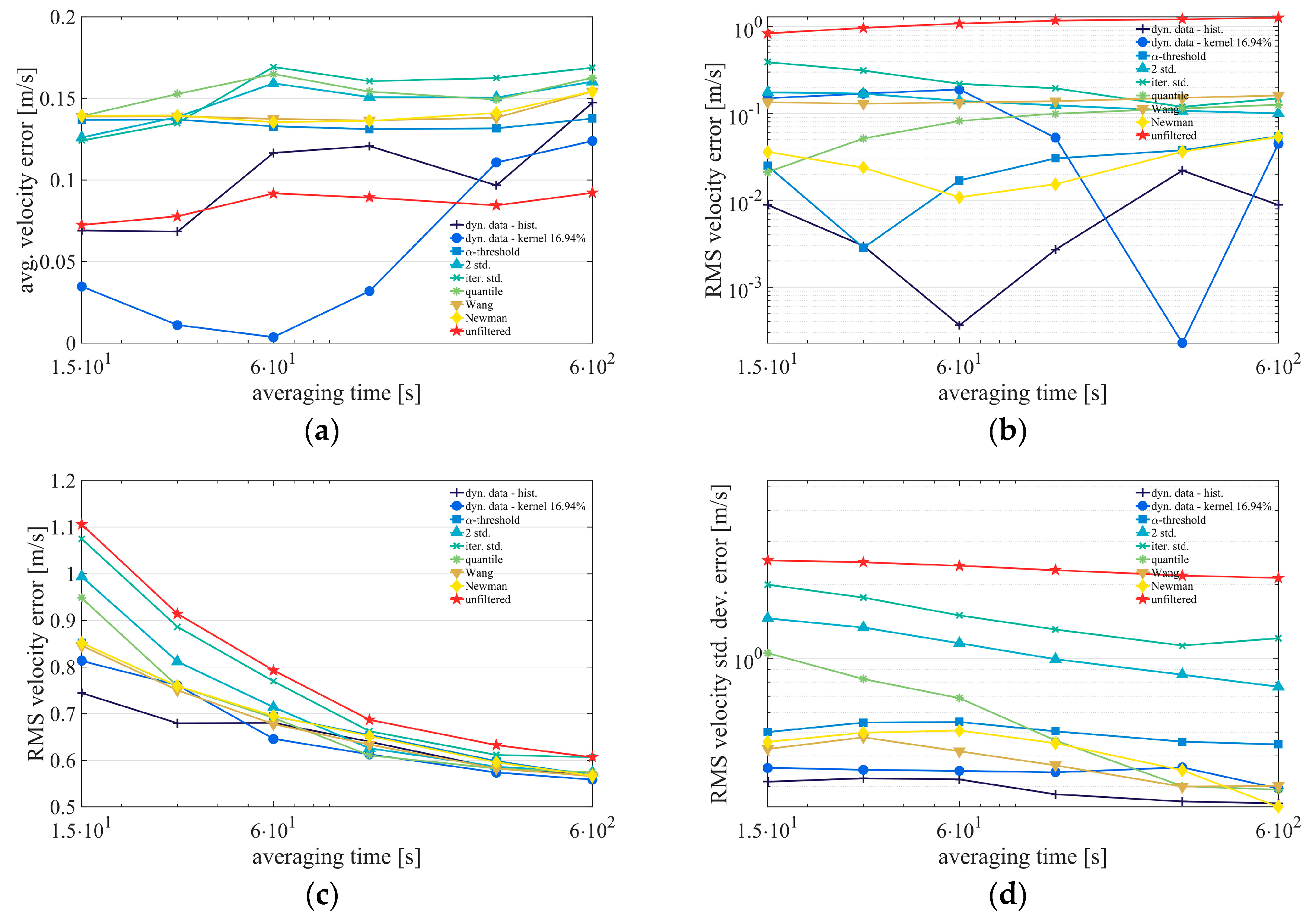
Figure A5 illustrate the influence of the averaging time for all filters on the resulting errors. Because the dynamic filters are dependent on the normalisation time, the corresponding value of was chosen from Figure A2 and Figure A3. While all non-dynamic data filters are subjected relative comparable results for variable averaging times, the strongest impact can be seen for the RMS velocity error which decreases quadratically over .
Figure A2.
Visualisation of the influence of the normalisation time and the averaging time on the resulting error of staring mode LiDAR data from 04.01.2014 7:30 h (UTC) till 05.01.2014 7:30 h (UTC) from the histogram-based dynamic data filter (a) Average velocity error; (b) average velocity standard deviation error; (c) RMS velocity error and (d) RMS velocity standard deviation error.
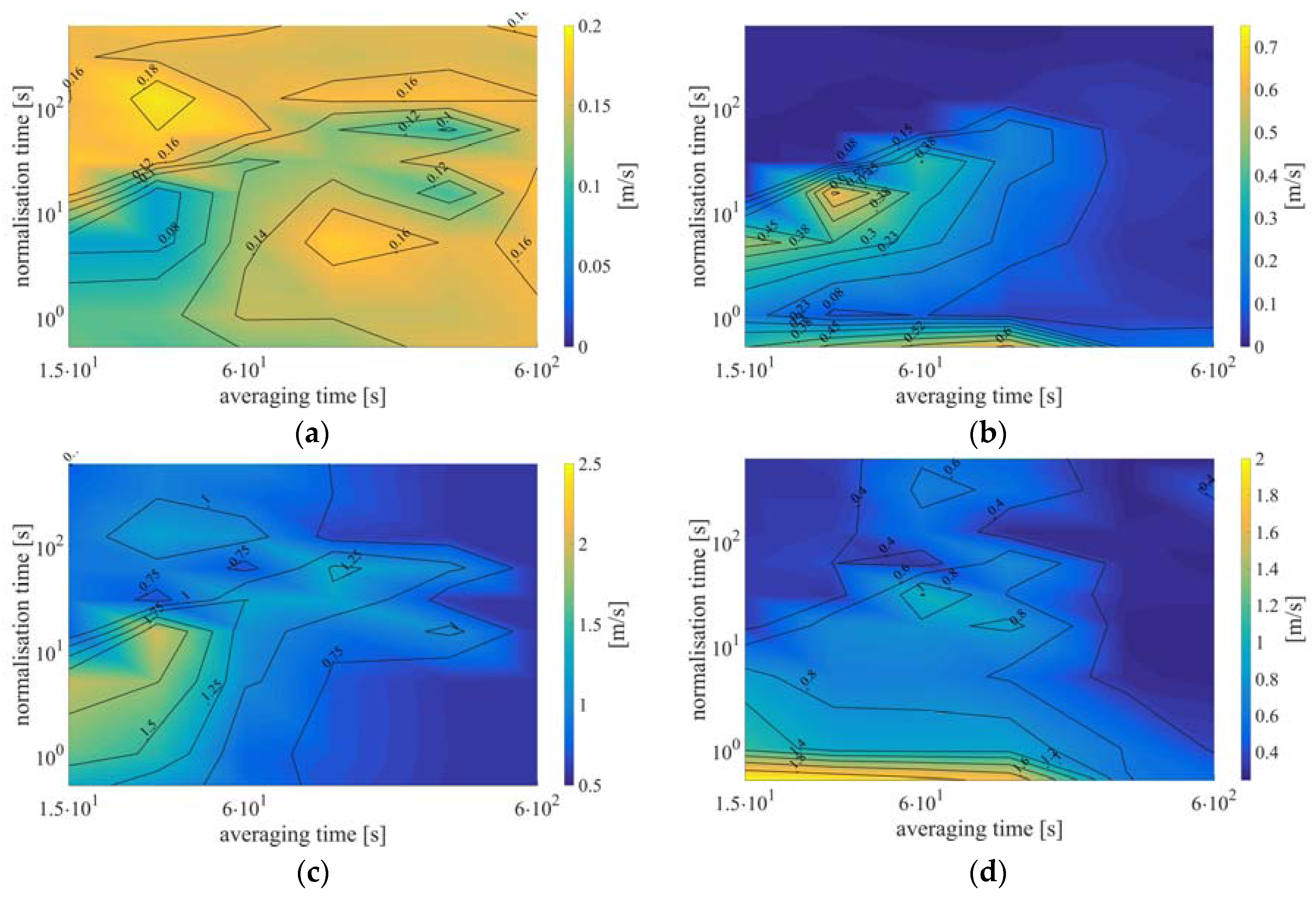
Figure A3.
Visualisation of the influence of the normalisation time and the averaging time on the resulting error of staring mode LiDAR data from 04.01.2014 7:30 h (UTC) till 05.01.2014 7:30 h (UTC) from the Gaussian kernel based dynamic data filter. (a) Average velocity error, (b) average velocity standard deviation error, (c) RMS velocity error and (d) RMS velocity standard deviation error.
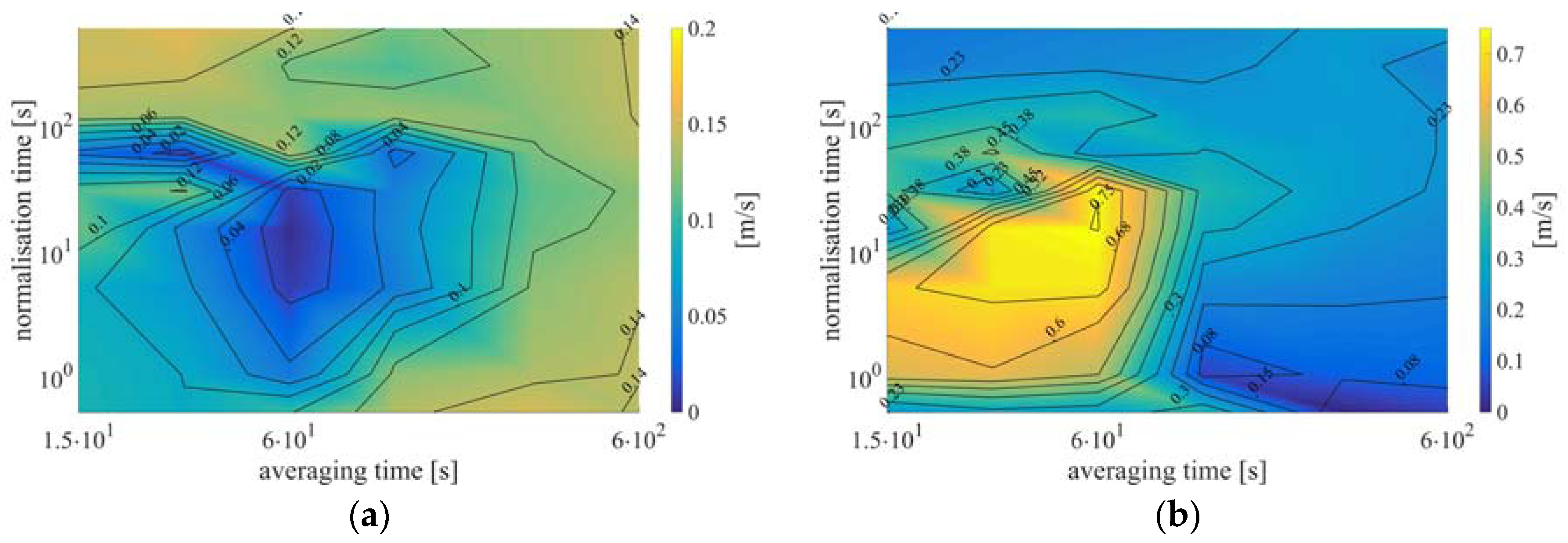
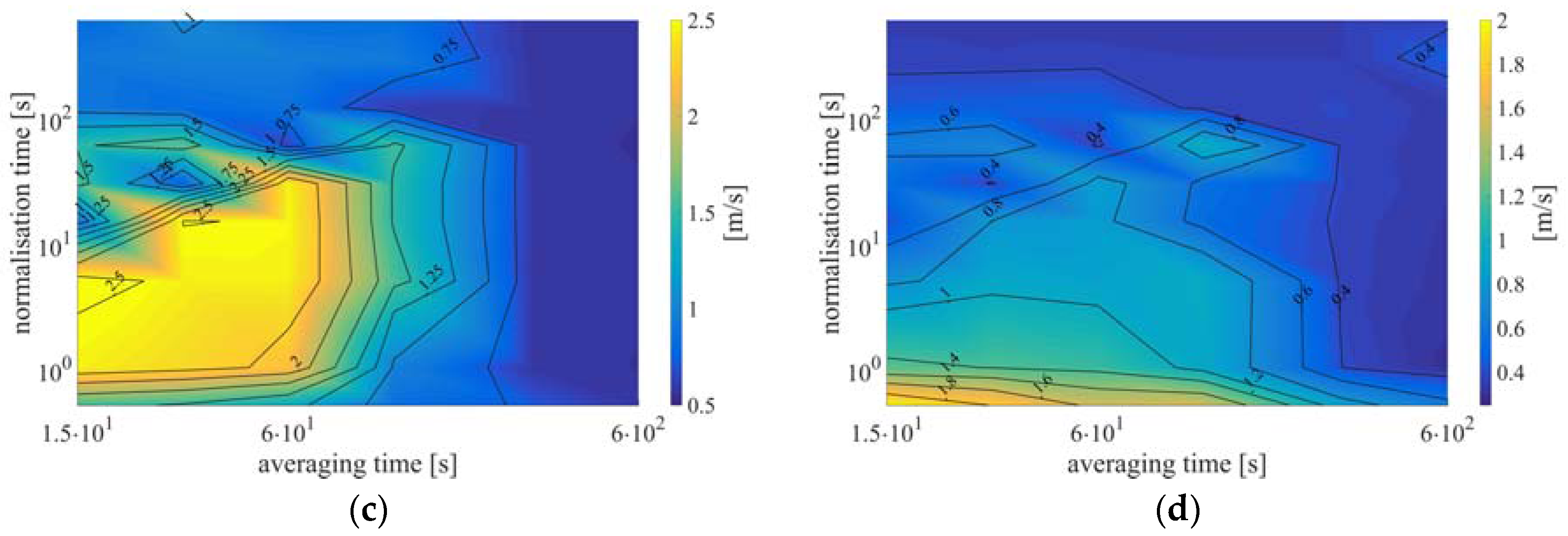
Figure A4.
Averaged and normalised error behaviour of the average velocity error, the RMS velocity error, the velocity standard deviation error and the RMS velocity standard deviation error of (a) the histogram-based dynamic data filter and (b) the Gaussian kernel based dynamic data filter. Staring mode LiDAR data from 04.01.2014 7:30 h (UTC) till 05.01.2014 7:30 h (UTC) form the basis for this calculation.

Figure A5.
Visualisation of the influence of the averaging time for all filters to the resulting errors. (a) Average velocity error, (b) average velocity standard deviation error, (c) RMS velocity error and (d) RMS velocity standard deviation error.
Figure A5.
Visualisation of the influence of the averaging time for all filters to the resulting errors. (a) Average velocity error, (b) average velocity standard deviation error, (c) RMS velocity error and (d) RMS velocity standard deviation error.

Appendix C. Comparison of Waked and Free Inflow
The following results were calculated in analogues way as described in Section 4.1. To obtain a better understanding of the filter behaviour, we distinguished between waked and free inflow conditions. We defined waked affected inflow wind direction from 110° to 180° and implied turbine wakes and the mast wake. This results can be seen in Table A1.
Free inflow conditions at the ultrasonic anemometer was captured in a wind direction range within 180–210°. Those results are provided in Table A2.

Table A1.
Comparison of different filtering methods applied on staring mode measurements for wake affected wind directions from 110° to 180°.
Table A1.
Comparison of different filtering methods applied on staring mode measurements for wake affected wind directions from 110° to 180°.
| Avg. Availability FINO1 | Avg. Availability All Ranges | Abs. Avg. Velocity Error | RMS Velocity Error | Abs. Avg. Velocity Std. Dev. Error | RMS Velocity Std. Dev. Error | |
|---|---|---|---|---|---|---|
| Dyn. data histogram | 89.9% | 91.6% | 0.50 m/s | 3.13 m/s | 0.21 m/s | 2.14 m/s |
| Dyn. data Gauss. kernel | 63.6% | 68.5% | 0.47 m/s | 2.91 m/s | 0.19 m/s | 1.10 m/s |
| CNR threshold | 76.1% | 83.5% | 0.75 m/s | 4.10 m/s | 0.50 m/s | 2.68 m/s |
| Std. dev. two sigma | 96.6% | 96.3% | 0.73 m/s | 3.28 m/s | 1.04 m/s | 3.50 m/s |
| Iterative std. dev. | 97.1% | 97.5% | 0.77 m/s | 3.26 m/s | 1.02 m/s | 4.03 m/s |
| Quartile filter | 92.5% | 93.3% | 0.61 m/s | 3.17m/s | 0.53 m/s | 3.28 m/s |
| Combined Wang | 72.1% | 79.3% | 0.68 m/s | 4.24 m/s | 0.05 m/s | 2.24 m/s |
| Combined Newman | 76.0% | 83.4% | 0.70 m/s | 4.10 m/s | 0.29 m/s | 2.56 m/s |
| No filter | 100% | 100% | 1.13 m/s | 3.31 m/s | 3.14 m/s | 4.87 m/s |
Table A2.
Comparison of different filtering methods applied on staring mode measurements for free inflow condition and wind directions from 180° to 210°.
Table A2.
Comparison of different filtering methods applied on staring mode measurements for free inflow condition and wind directions from 180° to 210°.
| Avg. Availability FINO1 | Avg. Availability All Ranges | Abs. Avg. Velocity Error | RMS Velocity Error | Abs. Avg. Velocity Std. Dev. Error | RMS Velocity Std. Dev. Error | |
|---|---|---|---|---|---|---|
| Dyn. data histogram | 89.3% | 90.1% | 0.07 m/s | 0.81 m/s | 0.04 m/s | 1.26 m/s |
| Dyn. data Gauss. kernel | 70.9% | 72.6% | 0.02 m/s | 0.91 m/s | 0.18 m/s | 0.63 m/s |
| CNR threshold | 89.3% | 92.8% | 0.13 m/s | 0.90 m/s | 0.17 m/s | 1.43 m/s |
| Std. dev. two sigma | 96.1% | 96.0% | 0.24 m/s | 1.32 m/s | 0.32 m/s | 2.11 m/s |
| Iterative std. dev. | 99.2% | 99.4% | 0.28 m/s | 1.39 m/s | 0.45 m/s | 2.48 m/s |
| Quartile filter | 94.3% | 94.6% | 0.18 m/s | 1.21 m/s | 0.09 m/s | 1.86 m/s |
| Combined Wang | 84.5% | 87.8% | 0.08 m/s | 0.80 m/s | 0.10 m/s | 1.06 m/s |
| Combined Newman | 89.2% | 92.7% | 0.11 m/s | 0.88 m/s | 0.05 m/s | 1.31 m/s |
| No filter | 100% | 100% | 0.38 m/s | 1.44 m/s | 1.03 m/s | 2.87 m/s |
References
- Grund, C.J.; Banta, R.M.; George, J.L.; Howell, J.N.; Post, M.J.; Richter, R.A.; Weickmann, A.M. High-resolution Doppler LiDAR for boundary-layer and cloud research. J. Atmos. Ocean. Technol. 2001, 18, 376–393. [Google Scholar] [CrossRef]
- Smith, D.A.; Harris, M.; Coffey, A.S.; Mikkelsen, T.; Jørgensen, H.E.; Mann, J.; Danielian, R. Wind LiDAR evaluation at the Danish wind test site in Høvsøre. Wind Energy 2006, 9, 87–93. [Google Scholar] [CrossRef]
- Käsler, Y.; Rahm, S.; Simmet, R.; Kühn, M. Wake measurements of a multi-MW wind turbine with coherent long-range pulsed Doppler wind LiDAR. J. Atmos. Ocean. Technol. 2010, 27, 1529–1532. [Google Scholar] [CrossRef]
- Lang, S.; Mckeogh, E. LIDAR and SODAR Measurements of Wind Speed and Direction in Upland Terrain for Wind Energy Purposes. Remote Sens. 2011, 3, 1871–1901. [Google Scholar] [CrossRef]
- Trujillo, J.J.; Bingöl, F.; Larsen, G.C.; Mann, J.; Kühn, M. Light detection and ranging measurements of wake dynamics. Part II: Two-dimensional scanning. Wind Energy 2011, 14, 61–75. [Google Scholar] [CrossRef]
- Trabucchi, D.; Trujillo, J.J.; Schneemann, J.; Bitter, M.; Kühn, M. Application of staring LiDARs to study the dynamics of wind turbine wakes. Met. Z. 2015, 6, 557–564. [Google Scholar] [CrossRef]
- Goyer, G.G.; Watson, R. The Laser and its Application to Meteorology. Bull. Am. Meteorol. Soc. 1963, 44, 564–575. [Google Scholar]
- Vickers, D.; Mahrt, L. Quality control and flux sampling problems for tower and aircraft data. J. Atmos. Ocean. Technol. 1997, 14, 512–526. [Google Scholar] [CrossRef]
- Frehlich, R. Effects of wind turbulence on coherent Doppler LiDAR performance. J. Atmos. Ocean. Techol. 1997, 14, 54–75. [Google Scholar] [CrossRef]
- Pal, S.; Haeffelin, M.; Batchvarova, E. Exploring a geophysical process-based attribution technique for the determination of the atmospheric boundary layer depth using aerosol LiDAR and near-surface meteorological measurements. J. Geophys. Res. Atmos. 2013, 118, 9277–9295. [Google Scholar] [CrossRef]
- Pal, S.; Lee, T.R.; Phelps, S.; De Wekker, S.F.J. Impact of atmospheric boundary layer depth variability and wind reversal on the diurnal variability of aerosol concentration at a valley site. Sci. Total. Environ. 2014. [Google Scholar] [CrossRef] [PubMed]
- Hill, M.; Calhoun, R.; Fernando, H.J.S. Coplanar Doppler LiDAR Retrieval of Rotors from T-REX. AMETSOC JAS 2010, 67, 713–729. [Google Scholar] [CrossRef]
- Krishnamurthy, R.; Choukulkar, A.; Calhoun, R.; Fine, J.; Oliver, A.; Barr, K.S. Coherent Doppler LiDAR for wind farm characterization. Wind Energy 2013, 16, 189–206. [Google Scholar] [CrossRef]
- Newsom, R.K.; Berg, L.K.; Shaw, W.J.; Fischer, M.L. Turbine-scale wind field measurements using dual-Doppler LiDAR. Wind Energy 2015, 18, 219–235. [Google Scholar] [CrossRef]
- Gryning, S.-E.; Floors, R.; Peña, A.; Batchvarova, E.; Brümmer, B. Weibull Wind-Speed Distribution Parameters Derived from a Combination of Wind-LiDAR and Tall-Mast Measurements Over Land, Coastal and Marine Sites. Bound.-Layer Meteorol. 2016, 159, 329–348. [Google Scholar] [CrossRef]
- Newman, J.F.; Klein, P.M.; Wharton, S.; Sathe, A.; Bonin, T.A.; Chilson, P.B.; Muschinski, A. Evaluation of three LiDAR scanning strategies for turbulence measurements. Atmos. Meas. Tech. 2016, 9, 1993–2013. [Google Scholar] [CrossRef]
- Wang, H.; Barthelmie, R.; Clifton, A.; Pryor, S.C. Wind Measurements from Arc Scans with Doppler Wind LiDAR. J. Atmos. Ocean. Technol. 2015, 32, 2024–2040. [Google Scholar] [CrossRef]
- Meyer Forsting, A.R.; Troldborg, N. A finite difference approach to despiking in-stationary velocity data—Tested on a triple-LiDAR. J. Phys. IOP Conf. Ser. 2016, 753, 072017. [Google Scholar] [CrossRef]
- Højstrup, J. A statistical data screening procedure. Meas. Sci. Technol. 1993, 4, 153–157. [Google Scholar] [CrossRef]
- Hoaglin, D.C.; Mosteller, F.; Tukey, J.W. Wiley Series in Probability and Mathematical Statistics. In Understanding Robust and Exploratory Data Analysis; Wiley: Hoboken, NJ, USA, 1983; Volume 84, p. 447. [Google Scholar]
- Botev, Z.I.; Grotowski, J.F.; Kroese, D.P. Kernel density estimation via diffusion. Ann. Stat. 2010, 38, 2916–2957. [Google Scholar] [CrossRef]
- Scott, D.W. On optimal and data-based histograms. Biometrika 1979, 66, 605–610. [Google Scholar] [CrossRef]
- Morales, A.; Wächter, M.; Peinke, J. Characterization of wind turbulence by higher-order statistics. Wind Energy 2011, 15, 391–406. [Google Scholar] [CrossRef]
- Shapiro, S.S.; Wilk, M.B. An analysis of variance test for normality. Biometrika 1965, 52, 591. [Google Scholar] [CrossRef]
- Bastine, D.; Wächter, M.; Peinke, J.; Trabucchi, D.; Kühn, M. Characterizing Wake Turbulence with Staring LiDAR Measurements. J. Phys. IOP Conf. Ser. 2015, 625. [Google Scholar] [CrossRef]
- Schmidt, M.; Trujillo, J.J.; Kühn, M. Orientation correction of wind direction measurements by means of staring LiDAR. J. Phys. IOP Conf. Ser. 2016, 749. [Google Scholar] [CrossRef]
- Westerhellweg, A.; Neumann, T.; Riedel, V. FINO1 Mast Correction. 2012 DEWI Magazin 60–66. Available online: http://www.dewi.de/dewi_res/fileadmin/pdf/publications/Magazin_40/09.pdf (accessed on 9 December 2016).
- Sathe, A.; Mann, J. A review of turbulence measurements using ground-based wind LiDARs. Atmos. Meas. Tech. 2013, 6, 3147–3167. [Google Scholar] [CrossRef]
- Sathe, A.; Mann, J.; Gottschall, J.; Courtney, M.S. Can wind LiDARs measure turbulence? J. Atmos. Ocean. Technol. 2011, 28, 853–868. [Google Scholar] [CrossRef]
- Schneemann, J.; Trabucchi, D.; Trujillo, J.J.; Kühn, M. Comparing measurements of horizontal wind speed of a 2D Multi-LiDAR and a cup anemometer. J. Phys. Conf. Ser. 2012. [Google Scholar] [CrossRef]
- Klaas, T.; Pauscher, L.; Callies, D. LiDAR-mast deviations in complex terrain and their simulation using CFD. Meteorol. Z. 2015, 24, 591–603. [Google Scholar] [CrossRef]
- Pauscher, L.; Vasiljevic, N.; Callies, D.; Lea, G.; Mann, J.; Klaas, T.; Hieronimus, J.; Gottschall, J.; Schwesig, A.; Kühn, M.; Courtney, M. An Inter-Comparison Study of Multi- and DBS LiDAR Measurements in Complex Terrain. Remote Sens. 2016, 8, 782. [Google Scholar] [CrossRef]
- Peña, A.; Mann, J.; Dimitrov, N. Turbulence characterization from a forward-looking nacelle LiDAR. Wind Energy Sci. 2016. [Google Scholar] [CrossRef]
- Boquet, M.; Royer, P.; Cariou, J.-P.; Matcha, M. Simulations of Doppler LiDAR Measurements Range and Data Availability. J. Atmos. Ocean. Technol. 2016. [CrossRef]
Figure 1.
Example of a staring mode LiDAR measurement in the diagram for a duration of 30 min in distances in the range of 361 m to 2911 m. (a) Blue points represent single measurements points, the red horizontal line indicates the lower CNR-threshold of −24 dB. (b) Visualisation of data density of measurement point distribution. Colours indicate different values of frequency distribution.
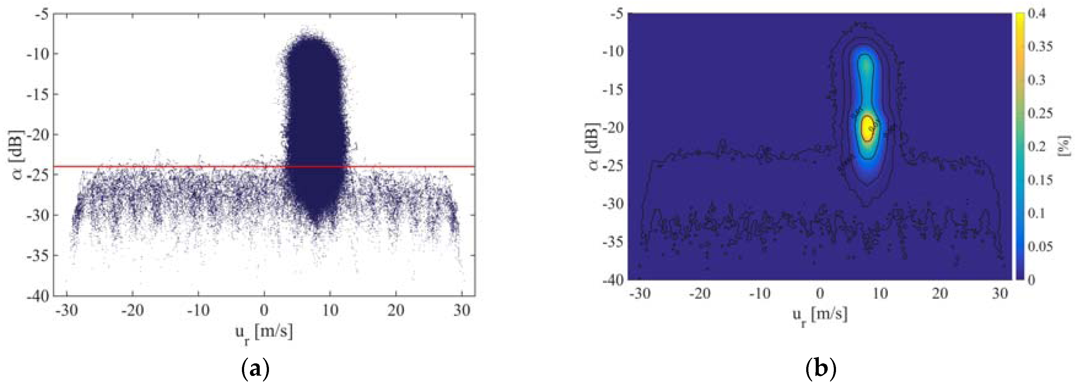
Figure 2.
Visualisation of segmentation of the overall filtering time interval in normalisation intervals .
Figure 2.
Visualisation of segmentation of the overall filtering time interval in normalisation intervals .

Figure 3.
Example of data-density distribution of a 30-min time interval of LiDAR staring mode measurements in the original frames of reference. Iso-lines show levels of probability of occurrence of the measurement with in a bin of 0.32 m/s width and 0.2 dB height.
Figure 3.
Example of data-density distribution of a 30-min time interval of LiDAR staring mode measurements in the original frames of reference. Iso-lines show levels of probability of occurrence of the measurement with in a bin of 0.32 m/s width and 0.2 dB height.
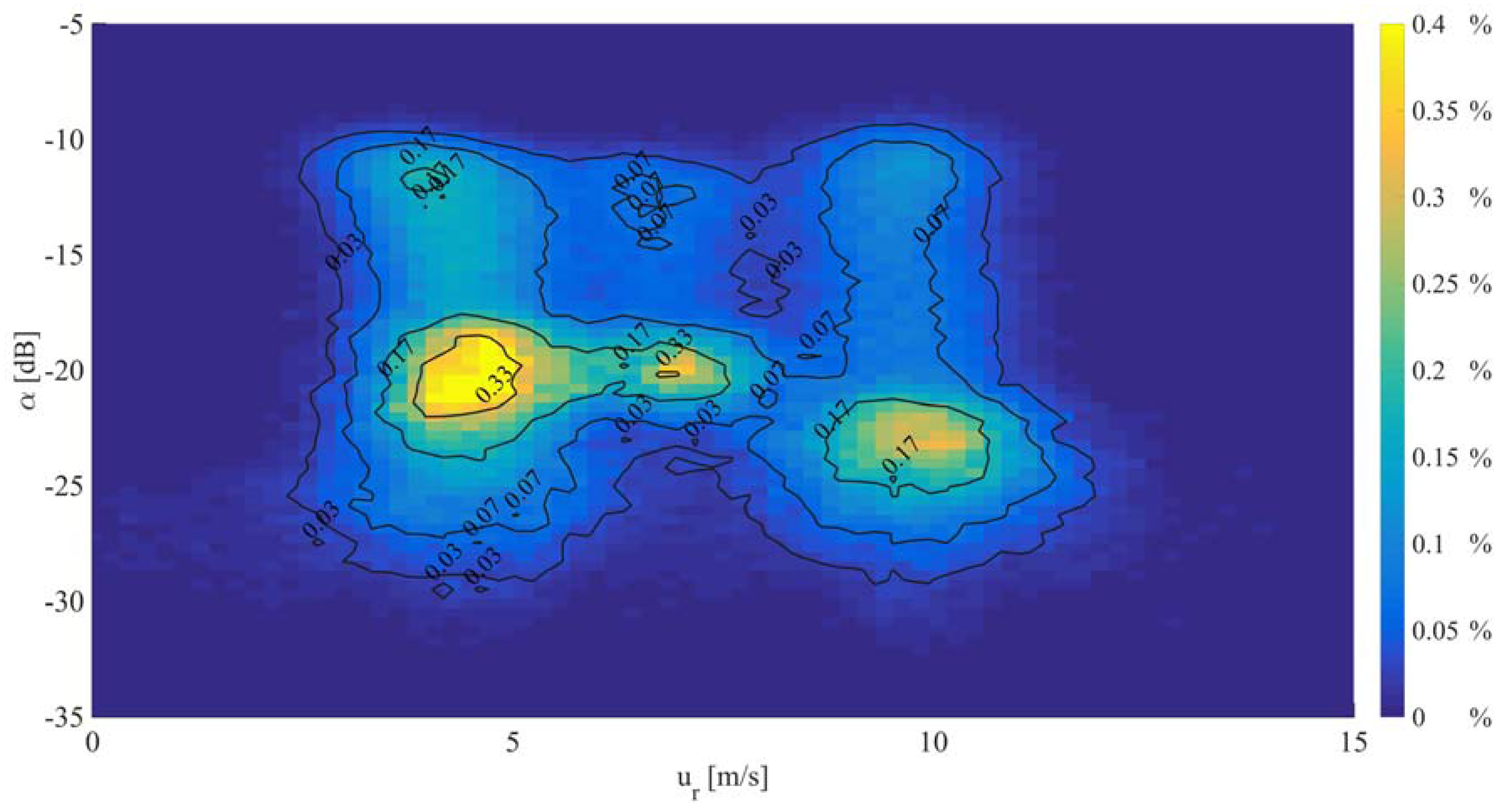
Figure 4.
Visualisation of different normalisation times of the LiDAR data distribution in the normalised frame of reference (a) (b) (c) (d) (e) (f) (g) (h) (i) .
Figure 4.
Visualisation of different normalisation times of the LiDAR data distribution in the normalised frame of reference (a) (b) (c) (d) (e) (f) (g) (h) (i) .

Figure 5.
Behaviour of parametrisation of fitted bi-variate Gaussian distribution of data density in relation to the different normalisation time intervals . The -axis fitted standard deviation is shown in turquoise, -axis fitted standard deviation in dark blue, the maximum probability of occurrence in green and the residual of the original and the fitted data distribution.
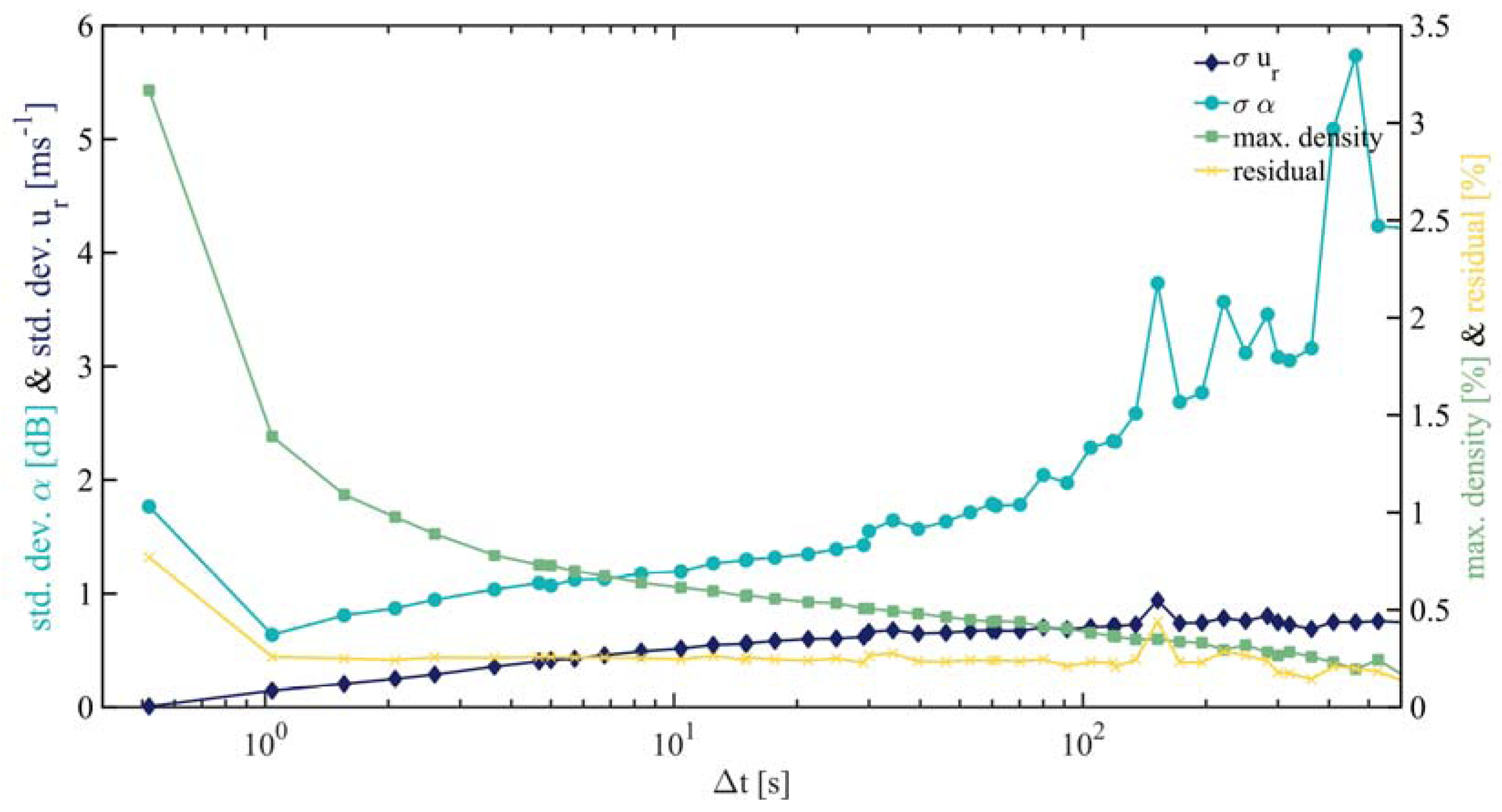
Figure 6.
Layout of the wind farm “alpha ventus” with measurement geometry of staring mode LiDAR with an azimuthal orientation of 306.47° and an elevation of 0.2° (red). Crosses represent wind turbines, the circle the platform FINO1 and the square the substation AV0. The measurement positions are indicated by the red line.

Figure 7.
Visualisation of the line-of-sight velocity turbulence intensity in dependency of the wind direction measured by the ultrasonic anemometer from 21.12.2013 15:35 h (UTC) till 19.01.2014 7:55 h (UTC). Gaps in the plot visualise unavailability of anemometer data. Individual 10 min mean values are shown in light blue whereas the binned averaged is marked in dark blue. Black vertical dashed lines indicate the wind direction of possible wake shading of the anemometer on FINO1 based on geometrical correlations. The red line shows the perpendicular wind direction to the azimuthal orientation of the laser beam.

Figure 8.
Histogram of 10 min averaged ultrasonic anemometer inflow conditions from 21.12.2013 15:35 h (UTC) till 19.01.2014 7:55 h (UTC) (a) horizontal wind speed in the meteorological reference frame is marked in dark blue, whereas the LiDAR laser beam projected wind speed (Equation (17)) is shown in green. The bin width is 1 m/s, (b) wind direction with a bin width of 3°.

Figure 9.
Time series of the 10 min averaged wind direction measured by the ultrasonic anemometer from 21.12.2013 15:35 h (UTC) till 19.01.2014 7:55 h (UTC). Gaps in the plot demonstrate unavailability of LiDAR data. Horizontal lines indicate the wind direction of possible wake shading of the anemometer on FINO1 based on geometrical correlations.

Figure 10.
Data availability of staring mode measurements for different filter methods. (a) time dependent behaviour for range at 2864 m and (b) averaged data availability over all ranges. The dashed line marks the distance of the anemometer at FINO1.
Figure 10.
Data availability of staring mode measurements for different filter methods. (a) time dependent behaviour for range at 2864 m and (b) averaged data availability over all ranges. The dashed line marks the distance of the anemometer at FINO1.
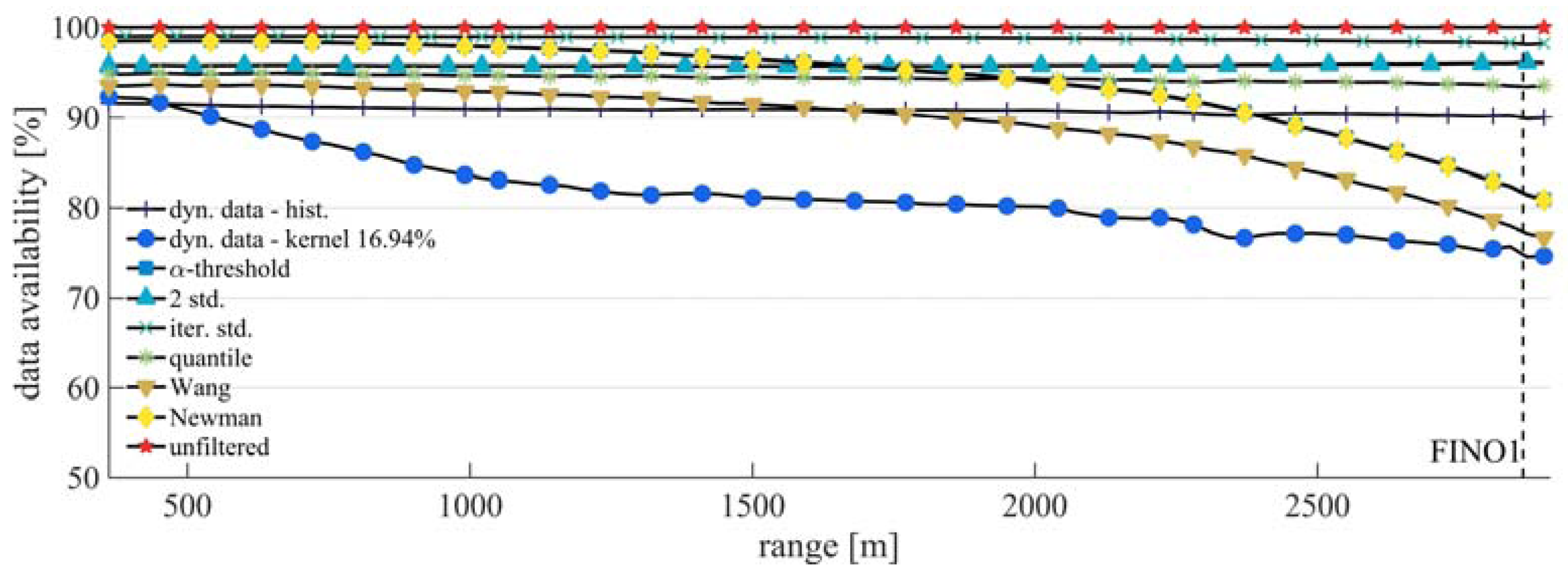
Figure 11.
Absolute error of staring mode measurements in dependency of data availability. Markers represent 10 min values of (a) the velocity error and (b) the velocity standard deviation.
Figure 11.
Absolute error of staring mode measurements in dependency of data availability. Markers represent 10 min values of (a) the velocity error and (b) the velocity standard deviation.

Figure 12.
Behaviour of the 10 min averaged filtered staring mode measurements of (a) the projected wind speed over time; (b) the standard deviation over time; (c) average wind speed error over wind direction; (d) average standard deviation error over wind direction. Vertical dashed lines indicate the wind direction of possible wake shading of the anemometer on FINO1 based on geometrical correlations.
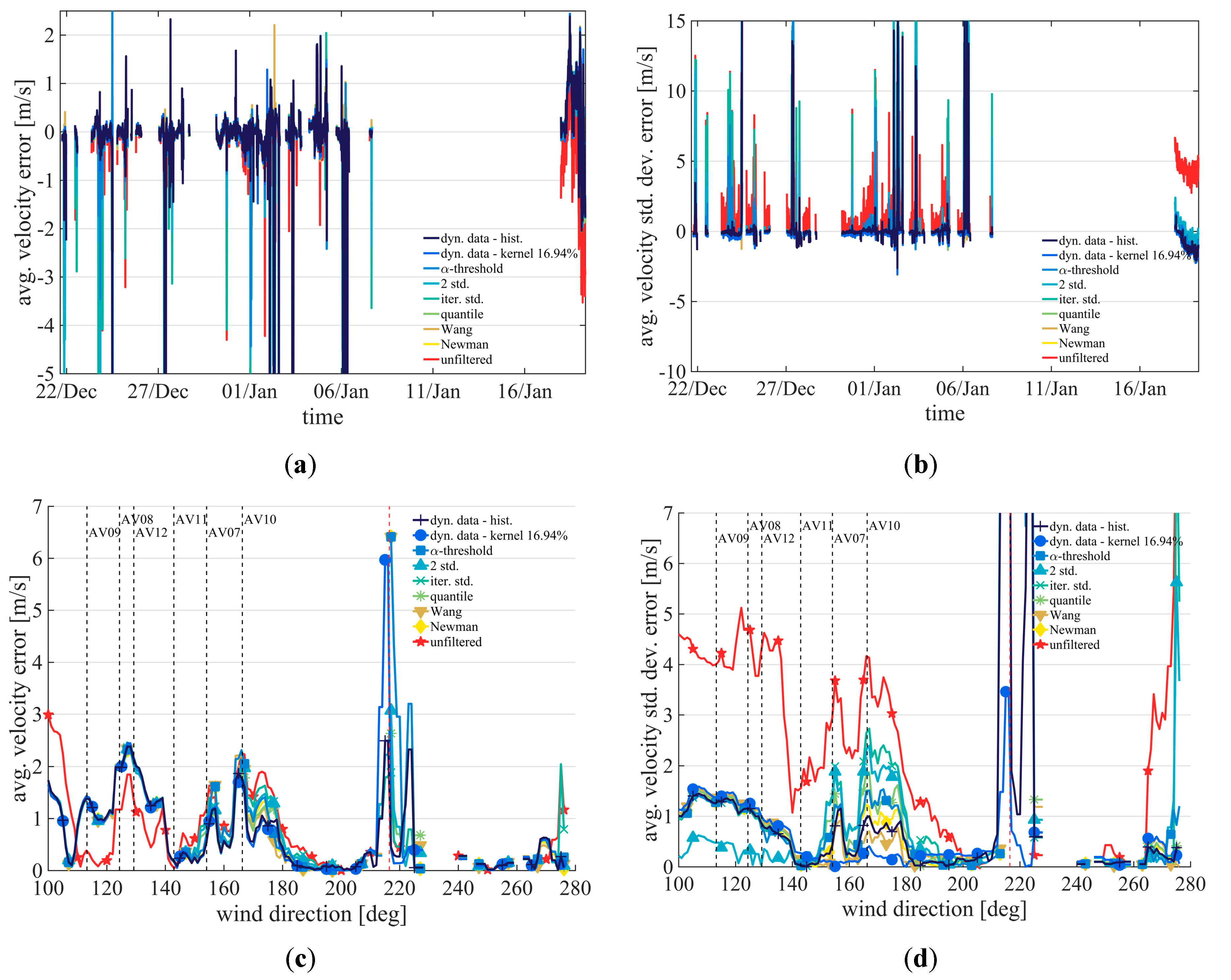
Figure 13.
Behaviour of the 10 min averaged filtered staring mode measurements of (a) the projected wind speed over time, (b) the standard deviation over time, (c) average wind speed error over time, (d) standard deviation error over time.
Figure 13.
Behaviour of the 10 min averaged filtered staring mode measurements of (a) the projected wind speed over time, (b) the standard deviation over time, (c) average wind speed error over time, (d) standard deviation error over time.
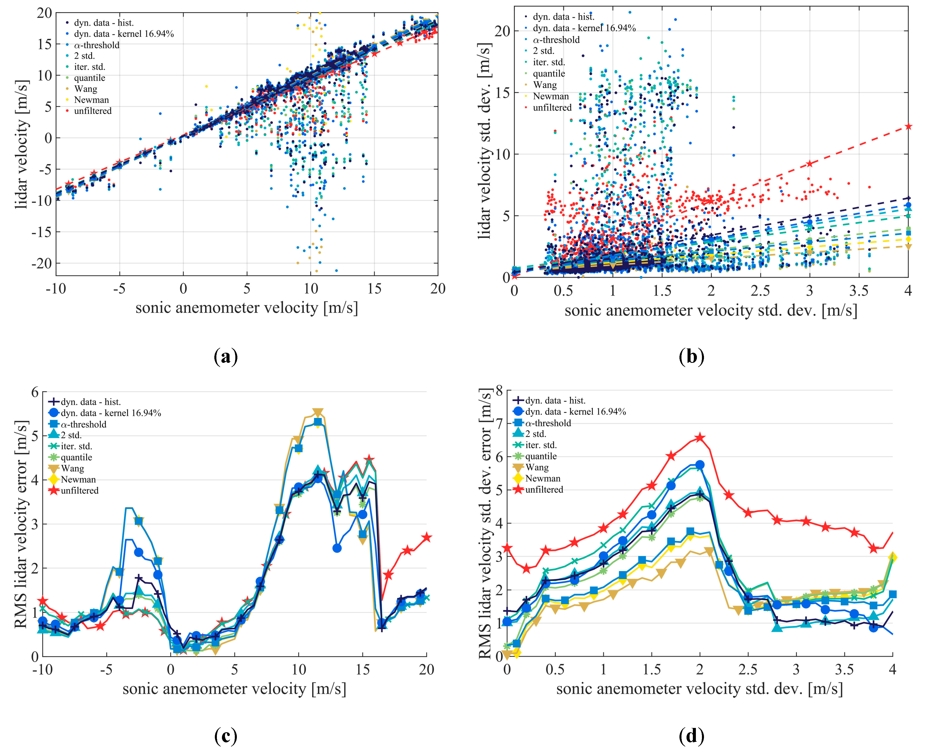
Figure 14.
Histogram in double logarithmic scaling with exponential increasing bin width of the (a) absolute average velocity error and (b) the absolute velocity standard deviation error. Vertical dashed lines indicate the centre of a fitted Gaussian curve.
Figure 14.
Histogram in double logarithmic scaling with exponential increasing bin width of the (a) absolute average velocity error and (b) the absolute velocity standard deviation error. Vertical dashed lines indicate the centre of a fitted Gaussian curve.
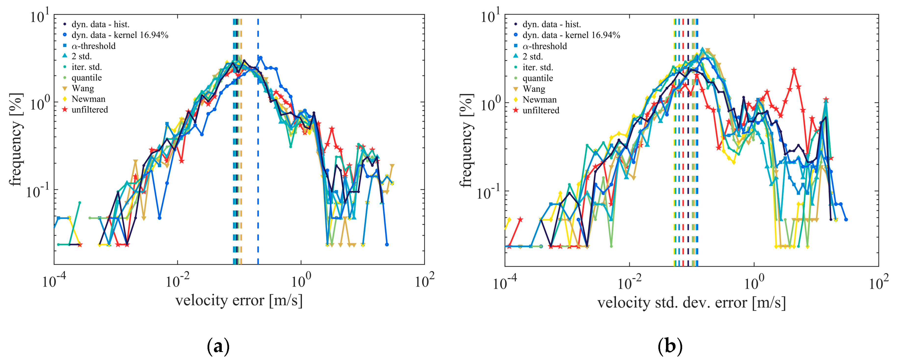
Figure 15.
Influence of maximum error threshold to the resulting error (a) RMS velocity error over velocity error threshold and (b) RMS velocity standard deviation error over velocity standard deviation error threshold.
Figure 15.
Influence of maximum error threshold to the resulting error (a) RMS velocity error over velocity error threshold and (b) RMS velocity standard deviation error over velocity standard deviation error threshold.
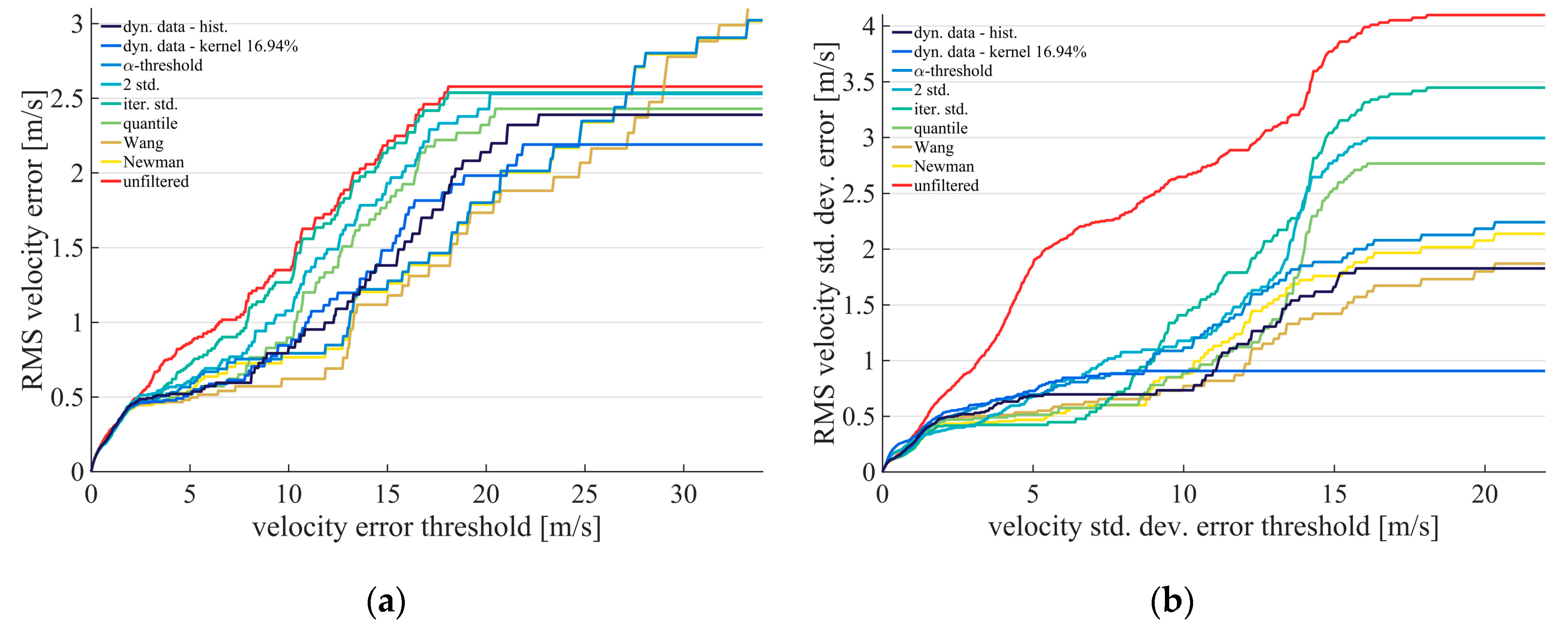
Figure 16.
Influence of different filtering methods on a 10 min averaged horizontal LiDAR scans. (1st column) radial speed, (2nd column) CNR mapping, (3rd column) standard deviation of radial speed. (a–c) histogram-based dynamic data filter, (d–f) Gaussian kernel based dynamic data filter, (g–i) CNR-threshold filter, (j–l) combined filter approach by Wang et al. (m–o) combined filter approach by Newman et al. (p–r) unfiltered.
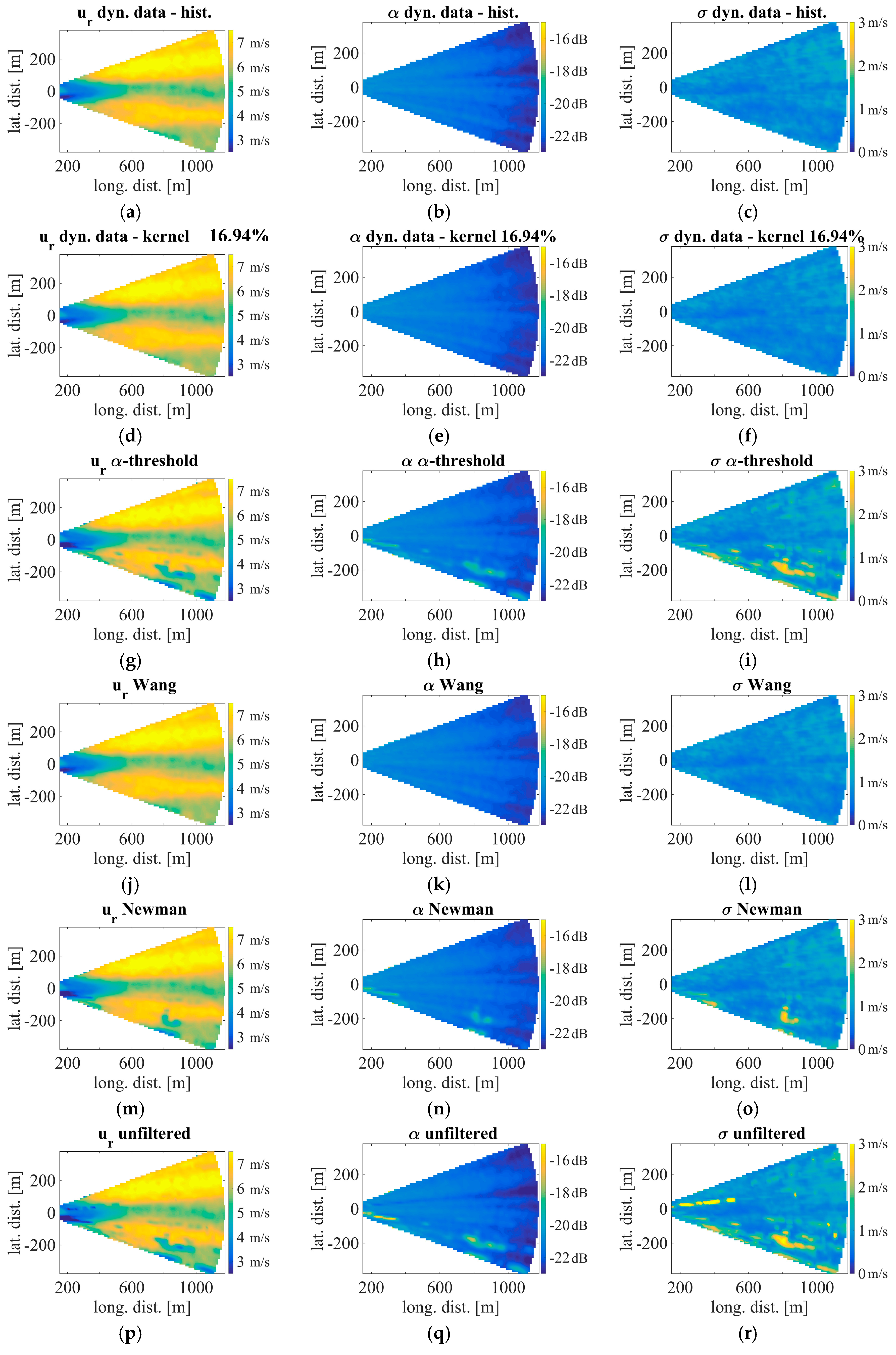
Figure 17.
Results of application of different filtering methods in the diagram. (a) histogram-based dynamic data filter, (b) Gaussian kernel based dynamic data filter, (c) CNR-threshold filter, (d) two sigma standard deviation filter, (e) iterative standard deviation filter, (f) interquartile-range, (g) combined filter approach by Wang et al. (h) combined filter approach by Newman et al. (i) no filtering.
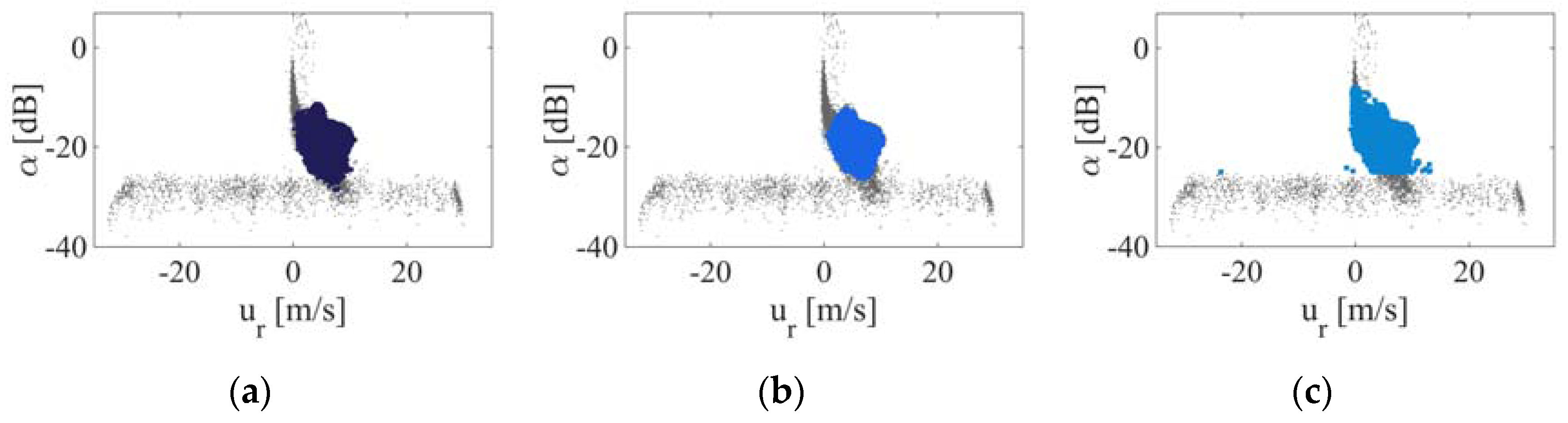

Figure 18.
Visualisation of the data density distribution of Stream Line XR PPI data from 31.10.2016 00:00 h (UTC) till 31.10.2016 00:30 h (UTC) in (a) diagram and (b) in the normalised reference frame.
Figure 18.
Visualisation of the data density distribution of Stream Line XR PPI data from 31.10.2016 00:00 h (UTC) till 31.10.2016 00:30 h (UTC) in (a) diagram and (b) in the normalised reference frame.
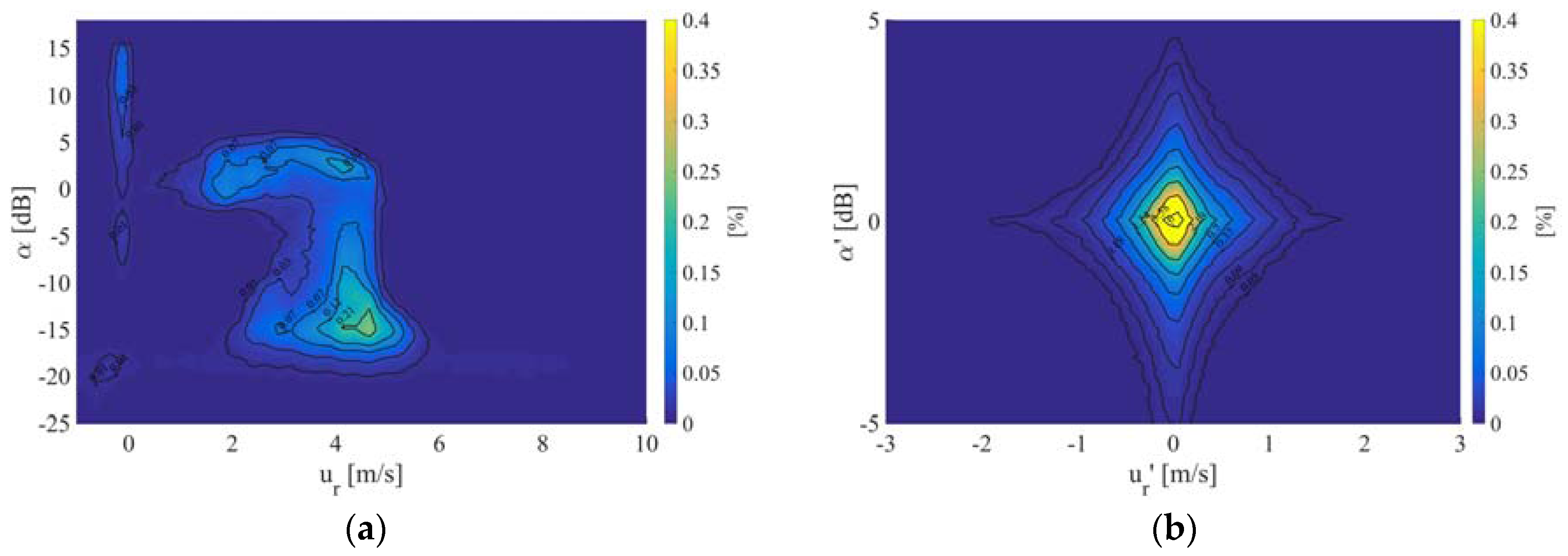
Table 1.
Comparison of different filtering methods applied on staring mode measurements from 21.12.2013 15:35 h (UTC) till 19.01.2014 7:55 h (UTC) for all wind directions.
Table 1.
Comparison of different filtering methods applied on staring mode measurements from 21.12.2013 15:35 h (UTC) till 19.01.2014 7:55 h (UTC) for all wind directions.
| Avg. Availability FINO1 | Avg. Availability All Ranges | Abs. Avg. Velocity Error | RMS Velocity Error | Abs. Avg. Velocity Std. Dev. Error | RMS Velocity Std. Dev. Error | |
|---|---|---|---|---|---|---|
| Dyn. data histogram | 90.0% | 90.4% | 0.34 m/s | 2.38 m/s | 0.14 m/s | 1.82 m/s |
| Dyn. data Gauss. kernel | 75.1% | 78.2% | 0.30 m/s | 2.10 m/s | 0.18 m/s | 0.90 m/s |
| CNR threshold | 81.9% | 87.6% | 0.45 m/s | 3.02 m/s | 0.36 m/s | 2.24 m/s |
| Std. dev. two sigma | 96.2% | 95.9% | 0.49 m/s | 2.50 m/s | 0.73 m/s | 3.00 m/s |
| Iterative std. dev. | 98.1% | 98.5% | 0.54 m/s | 2.54 m/s | 0.79 m/s | 3.45 m/s |
| Quartile filter | 93.5% | 94.0% | 0.40 m/s | 2.42 m/s | 0.35 m/s | 2.77 m/s |
| Combined Wang | 77.5% | 83.0% | 0.40 m/s | 3.10 m/s | 0.00 m/s | 1.87 m/s |
| Combined Newman | 81.8% | 87.5% | 0.42 m/s | 3.02 m/s | 0.20 m/s | 2.14 m/s |
| No filter | 100% | 100% | 0.76 m/s | 2.58 m/s | 2.17 m/s | 4.10 m/s |
Table 2.
Correlations and residuals of the linear regression between the ultrasonic anemometer and the LiDAR for the velocity and the standard deviation of the velocity. From 21.12.2013 15:35 h (UTC) till 19.01.2014 7:55 h (UTC) for all wind directions.
Table 2.
Correlations and residuals of the linear regression between the ultrasonic anemometer and the LiDAR for the velocity and the standard deviation of the velocity. From 21.12.2013 15:35 h (UTC) till 19.01.2014 7:55 h (UTC) for all wind directions.
| Dyn. Data Hist. | Dyn. Data Gauss. | CNR Thres-hold | Std. Dev. | Iter. Std | Quartile | Wang | Newman | Unfiltered | |
|---|---|---|---|---|---|---|---|---|---|
| Velocity | |||||||||
| Reg. slope | 0.92 | 0.95 | 0.96 | 0.92 | 0.91 | 0.93 | 0.97 | 0.97 | 0.86 |
| Offset [m/s] | 0.31 | 0.26 | 0.22 | 0.33 | 0.32 | 0.32 | 0.22 | 0.22 | 0.44 |
| R2 | 0.85 | 0.84 | 0.90 | 0.83 | 0.79 | 0.85 | 0.90 | 0.90 | 0.78 |
| Velocity std. dev. | |||||||||
| Reg. slope | 1.50 | 1.39 | 0.73 | 1.27 | 1.05 | 0.86 | 0.50 | 0.62 | 3.04 |
| Offset [m/s] | 0.42 | 0.33 | 0.63 | 0.45 | 0.74 | 0.49 | 0.50 | 0.58 | 0.08 |
| R2 | 0.06 | 0.04 | 0.02 | 0.04 | 0.02 | 0.02 | 0.01 | 0.01 | 0.15 |
Table 3.
Most probable velocity and standard deviation error of fitted double log-normal distribution to 10 min error histogram.
Table 3.
Most probable velocity and standard deviation error of fitted double log-normal distribution to 10 min error histogram.
| Dyn. Data Hist. | Dyn. Data Gauss. | CNR Thres-hold | Std. Dev. | Iter. Std | Quartile | Wang | Newman | Unfiltered | |
|---|---|---|---|---|---|---|---|---|---|
| Velocity [m/s] | 0.09 | 0.20 | 0.09 | 0.09 | 0.09 | 0.10 | 0.11 | 0.09 | 0.11 |
| Vel. std. dev. [m/s] | 0.09 | 0.12 | 0.06 | 0.12 | 0.06 | 0.10 | 0.11 | 0.06 | 0.07 |
© 2017 by the authors. Licensee MDPI, Basel, Switzerland. This article is an open access article distributed under the terms and conditions of the Creative Commons Attribution (CC BY) license (http://creativecommons.org/licenses/by/4.0/).
Share and Cite
MDPI and ACS Style
Beck, H.; Kühn, M. Dynamic Data Filtering of Long-Range Doppler LiDAR Wind Speed Measurements. Remote Sens. 2017, 9, 561. https://doi.org/10.3390/rs9060561
AMA Style
Beck H, Kühn M. Dynamic Data Filtering of Long-Range Doppler LiDAR Wind Speed Measurements. Remote Sensing. 2017; 9(6):561. https://doi.org/10.3390/rs9060561
Chicago/Turabian StyleBeck, Hauke, and Martin Kühn. 2017. "Dynamic Data Filtering of Long-Range Doppler LiDAR Wind Speed Measurements" Remote Sensing 9, no. 6: 561. https://doi.org/10.3390/rs9060561
Note that from the first issue of 2016, this journal uses article numbers instead of page numbers. See further details here.