
An Automated Approach to Map Winter Cropped Area of Smallholder Farms across Large Scales Using MODIS Imagery


1
School of Natural Resources and Environment, University of Michigan, Ann Arbor, MI 48109, USA
2
Center for International Earth Science Information Network, Columbia University, Palisades, NY 10964, USA
3
Gund Institute of Environment and Rubenstein School of Environment and Natural Resources, University of Vermont, Burlington, VT 05405, USA
4
Woods Hole Research Center, Falmouth, MA 02540, USA
5
Department of Ecology, Evolution, and Environmental Biology, Columbia University, New York, NY 10027, USA
*
Author to whom correspondence should be addressed.
Remote Sens. 2017, 9(6), 566; https://doi.org/10.3390/rs9060566
Submission received: 9 March 2017
/
Revised: 27 May 2017
/
Accepted: 29 May 2017
/
Published: 6 June 2017
(This article belongs to the Special Issue Remote Sensing of Smallholder Subsistence Agriculture Using Satellites and UAVs)
Abstract
:Fine-scale agricultural statistics are an important tool for understanding trends in food production and their associated drivers, yet these data are rarely collected in smallholder systems. These statistics are particularly important for smallholder systems given the large amount of fine-scale heterogeneity in production that occurs in these regions. To overcome the lack of ground data, satellite data are often used to map fine-scale agricultural statistics. However, doing so is challenging for smallholder systems because of (1) complex sub-pixel heterogeneity; (2) little to no available calibration data; and (3) high amounts of cloud cover as most smallholder systems occur in the tropics. We develop an automated method termed the MODIS Scaling Approach (MSA) to map smallholder cropped area across large spatial and temporal scales using MODIS Enhanced Vegetation Index (EVI) satellite data. We use this method to map winter cropped area, a key measure of cropping intensity, across the Indian subcontinent annually from 2000–2001 to 2015–2016. The MSA defines a pixel as cropped based on winter growing season phenology and scales the percent of cropped area within a single MODIS pixel based on observed EVI values at peak phenology. We validated the result with eleven high-resolution scenes (spatial scale of 5 × 5 m2 or finer) that we classified into cropped versus non-cropped maps using training data collected by visual inspection of the high-resolution imagery. The MSA had moderate to high accuracies when validated using these eleven scenes across India (R2 ranging between 0.19 and 0.89 with an overall R2 of 0.71 across all sites). This method requires no calibration data, making it easy to implement across large spatial and temporal scales, with 100% spatial coverage due to the compositing of EVI to generate cloud-free data sets. The accuracies found in this study are similar to those of other studies that map crop production using automated methods and use no calibration data. To aid research on agricultural production at fine spatial scales in India, we make our annual winter crop maps from 2000–2001 to 2015–2016 at 1 × 1 km2 produced in this study publically available through the NASA Socioeconomic Data and Applications Center (SEDAC) hosted by the Center for International Earth Science Information Network (CIESIN) at Columbia University. We also make our R script available since it is likely that this method can be used to map smallholder agriculture in other regions across the globe given that our method performed well in disparate agro-ecologies across India.

1. Introduction
Long-term agricultural statistics are a valuable resource for understanding trends in food production and the factors that are associated with changes in production through time [1,2,3]. These types of analyses are critical for researchers and policy-makers to understand the factors limiting production and possible solutions to meet growing food demand over the coming decades [4]. Agricultural statistics exist for most countries, through government or FAO censuses, however, these data are typically coarse in resolution (e.g., state, national), particularly in the developing world [5]. While coarse-scale data can give a general understanding of production trends and the factors associated with changes in production through time, access to higher resolution data may help elucidate patterns of production that are important, but only visible at finer spatial scales, such as those caused by fine-scale differences in management or biophysical factors. Furthermore, finer spatial scale agricultural statistics can identify regions that currently face low production and need to be targeted with interventions to enhance food security over the coming decades.
Historically, researchers and practitioners have relied on remote sensing of satellite imagery to produce fine-scale agricultural statistics in regions where these statistics otherwise would not exist (e.g., [6,7]). Previous studies have successfully mapped both cropped area and yield, the two factors that contribute to overall production. However, most of the existing literature that has successfully mapped agricultural production across large scales has done so in regions with relatively large farm sizes that better match the spatial resolution of freely-available, long-term imagery such as, Landsat and MODIS than do farms in small-scale systems [8,9]. Less work has been done to develop similar methods and approaches that can accurately map agricultural production for smallholder fields (<2 ha), which is the main mode of production for most of the developing world [10]. There are three main challenges when using satellite imagery to map smallholder production across large spatial and temporal scales. First, the size of smallholder fields is typically smaller than the spatial resolution of freely-available satellite products, resulting in inaccurate production estimates due to mixed pixels [11]. Furthermore, little ground data exist in these regions to develop and calibrate models that translate satellite vegetation indices to measures of agricultural production [12,13]. Finally, many smallholder farms are located throughout the tropics where cloud cover can make it difficult to obtain satellite imagery during periods of peak crop growth [14].
Previous studies have mapped cropped area by identifying MODIS pixels that exhibit a hump-shaped phenology during the agricultural growing season of interest (e.g., [15,16]). Yet simply defining these pixels as cropped versus non-cropped results in significant over-prediction of cropped area for smallholder farms because some fields within each 250 × 250 m2 pixel may be uncropped [11]. To account for sub-pixel heterogeneity, our previous work developed an approach that uses moderate-resolution (30 × 30 m2) Landsat satellite data to quantify the percent that each 250 × 250 m2 MODIS pixel is cropped. More specifically, peak EVI values from MODIS satellite imagery were scaled between 0% and 100% cropped by identifying appropriate 0% and 100% end-member pixels using classified Landsat satellite imagery. While this method has been shown to accurately estimate smallholder cropped area (R2 > 0.75 at scales of 1 × 1 km2 and greater; [11]), it is difficult to automate this approach and apply it across large spatio-temporal scales because it requires (1) that Landsat satellite data are available in all years and regions of interest, which does not occur due to cloud cover (Figure S1); and (2) ground data to train and classify a Landsat satellite image, which often do not exist in smallholder systems [13]. To overcome these challenges, we develop a new automated approach, termed the MODIS Scaling Approach (MSA), that is theoretically similar, but does not require any satellite or ground data for calibration.
In this study, we use the MSA and MODIS EVI satellite data to map the winter cropped area of smallholder farms across India from 2000–2001 to 2015–2016. This method overcomes the three challenges described above by (1) accounting for sub-pixel heterogeneity; (2) being fully automated and not requiring any calibration data for training of our model; and (3) using MODIS satellite data which has few problems with missing data even in the tropics. This method builds on previous approaches that have been used to map cropped areas in smallholder systems [11,15] by accounting for sub-pixel heterogeneity and not requiring any training data, which allows us to apply the method across large spatial and temporal scales. We focus on mapping cropped area (rather than crop yield) because methods to derive cropped area are less sensitive to crop type, allowing us to develop nation-wide maps across regions that plant different crops. Furthermore, cropped area is an important measure of agricultural production [17]. We validate our cropped area estimates with estimates of cropped area defined using high-resolution satellite imagery in eleven sites across India. Given that farming systems across India are diverse in terms of crop type, climate, soil type, and topography [18], if our method is able to accurately map cropped area across all of India, it will likely will be able to accurately map cropped areas in other smallholder systems more generally.
2. Study Area
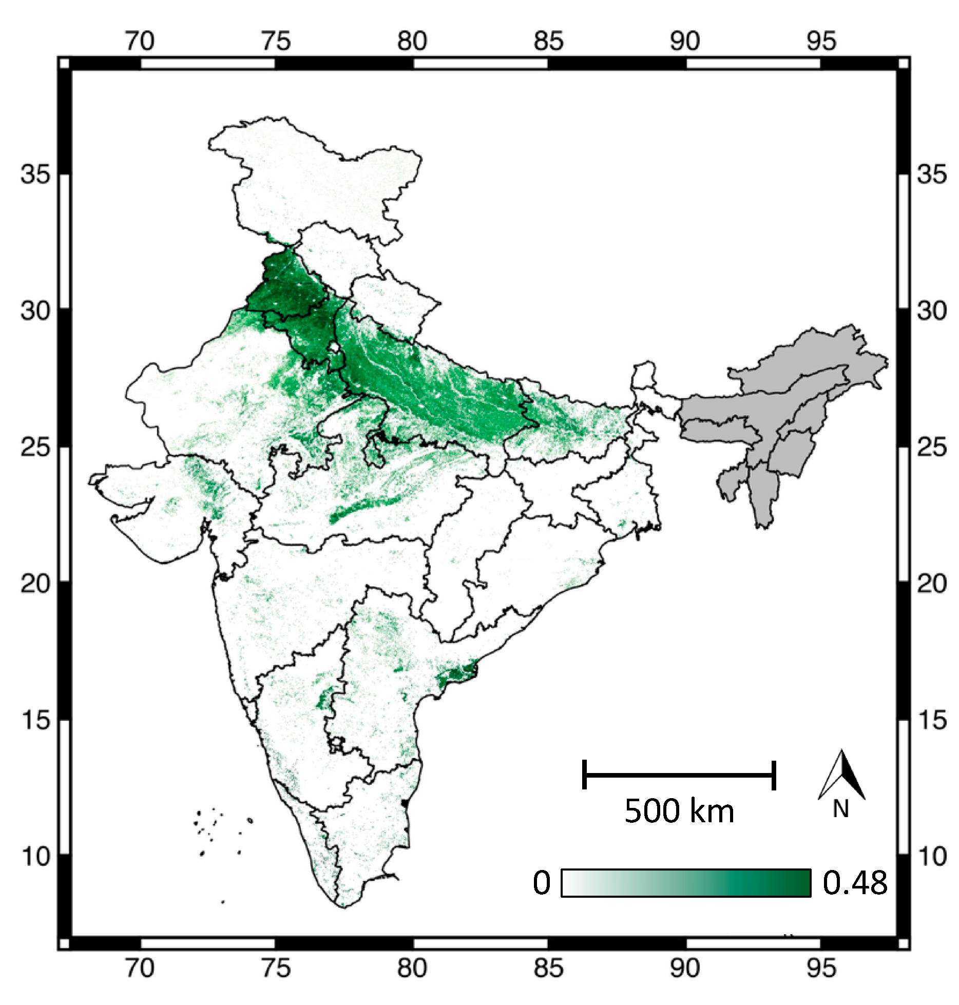
We focus on India because it is one of the largest global agricultural producers where the primary mode of production is smallholder agriculture [19]. Furthermore, high-resolution datasets on cropped area would be beneficial, given that India is expected to experience some of the greatest threats to food security over the coming decades [20,21]. Agriculture is a primary livelihood for over 70% of India’s rural population [22] with a large diversity in crop management across small spatial scales [23], necessitating higher-resolution statistics on cropped area than what is already available from census statistics. Our study is conducted across all states in India, excluding states in the northeast (Figure 1). We did not include Northeast India in our analysis as it was difficult to find cloud-free, high-resolution imagery for validation, and this region is significantly different in topography, soil type, and climate compared to the other areas in India for which we have validation data [18]. We conducted our analyses across forty-two agro-ecological subregions in India, which were defined as areas with similar soil, bioclimatic type, and physiographic context [18]. We specifically focused on the winter (rabi) cropping season for all analyses. The winter season is the second largest agricultural growing season across India, has less cloud cover compared to the main monsoon growing season, making it more feasible to use satellite data to map cropped area, is one of the main contributors to intensification through the Green Revolution, and likely has higher variability in cropped area through time than the monsoon season when farms are less water-limited.
3. Data and Methods
3.1. Data
To implement MSA, we downloaded 16-day composited, 250 × 250 m2 resolution, mosaicked MODIS Terra imagery for all of India from June 2000 to May 2016 from the IRI/LDEO Climate Data Library (http://www.climatedatalibrary.cl/). These data are LandDAAC MODIS version 5 EVI products compiled originally from the United States Geological Survey (USGS). We preferred the use of EVI over NDVI because it more effectively corrects for atmospheric contamination. Following the methods developed in [11], we used a cubic smoothing spline function on our EVI phenology data to remove any high-frequency noise. We then identified agricultural pixels by examining EVI phenology during the full winter growing season, from 1 October to 31 March [24,25] and defined a pixel as cropped if there was both an inflection point indicating green up after sowing as well as a period of peak greenness within the growing season window (Figure 2). We selected our time window based on crop calendars for the major winter crops in India and by examining MODIS EVI phenologies (Table S1, [26]). It is possible that some crops in some states (e.g., gram in Maharashtra, mustard in Rajasthan) were planted slightly earlier (in September) than our window so our algorithm may have missed some area planted under these specific region and crop combinations (up to 15% of area in Maharashtra and up to 37% of area in Rajasthan according to Indian district census statistics, [26]). Our method captures only annual crops planted during the winter (rabi) season and does not capture perennial crops or crops that were planted during the monsoon season and continue to grow throughout the winter season. Since there is little to no rainfall in the winter season to facilitate the growth of natural vegetation, we assumed that all pixels that exhibited green up and a peak in EVI represented cropped pixels.
3.2. Method
To conduct our scaling analysis, we identified appropriate 0% and 100% end-member pixels by assuming that the highest EVI value in a given agro-ecological subregion [18] represented a pixel that was 100% cropped and the lowest EVI value in a region represented a pixel that was 0% cropped; we only considered pixels that exhibited a hump-shaped phenology in EVI during the winter growing season (1 October to 31 March) for this selection of end-member values (Figure 2) to restrict this selection process to only cropped pixels. We base our end-member selection method on knowledge of vegetation growth in this region and on previous studies that have shown (1) bare soil typically has the lowest EVI values in an agricultural phenology, and (2) peak EVI values represent the maximum growth stage for crop cover [24,25,27]. In addition, our previous work that calibrated MODIS peak EVI based on the percent that the pixel was cropped according to classified Landsat satellite data showed that 0% cropped pixels were those with the lowest EVI and 100% cropped pixels were those with the largest peak EVI values within a given region [11]. Furthermore, we assume that differences in peak EVI values across pixels within an agro-ecological sub-region are primarily driven by cropped area as opposed to other factors, such as yield or crop type, that likely also influence peak EVI [11]. When we examine the relative contribution of cropped area versus yield to peak MODIS EVI in Bihar where we have high-resolution (2 × 2 m2) yield maps produced using micro-satellite data [12], we find that cropped area explains approximately 80% of the variation in peak MODIS EVI. Though we were unable to do a similar analysis comparing the percent of variation in peak MODIS EVI explained by cropped area versus crop type due to a lack of data, we believe this assumption is valid for two reasons. First, our previous work has shown that peak MODIS EVI is highly correlated with cropped area (R2 > 0.70), even in regions like Gujarat, where crop type is heterogeneous [11]. Second, previous studies that have used MODIS EVI to map crop type have found it difficult to classify crop type using peak EVI alone and instead rely on differences in EVI phenologies (e.g., [24,25]). To reduce the chance of selecting erroneously high and low EVI values, which may occur due to cloud contamination or other remaining high-frequency noise in our dataset, we selected the EVI values that were the 90% largest EVI value and the 10% smallest EVI value in a given region. We then linearly scaled all peak EVI values for each pixel between these end-member minimum and maximum EVI values. We calculated new scaling relationships for each individual year in our study to account for inter-annual variability in yield that may lead to differences in EVI values and for each agro-ecological sub-region to account for differences in crop type, climate, soil type, and topography, which may influence EVI [18,28,29].
3.3. High-Resolution Imagery Validation
We validated our cropped area estimates using single-date high-resolution Quickbird, WorldView-2, and RapidEye imagery across eleven different agricultural regions in India that represent a wide range in crop type, irrigation access, integration with market, and soil type (Figure S2; [18,30,31]). If our algorithm accurately quantifies the cropped area in these disparate regions, it is likely an accurate way to map cropped area across all of India. To obtain cropped area estimates from high-resolution imagery, we selected 50 cropped and 50 uncropped pixels based on visual inspection in each image and extracted the NDVI value for each of these points. We then used a regression tree to identify the NDVI value that differentiated cropped versus uncropped pixels, and classified the remainder of the image using this threshold value in a decision tree. We conducted validation at 1 × 1 km2, which previous work has shown to be the finest resolution for which MODIS data can be used to accurately map smallholder percent cropped area [11]. We aggregated the MODIS imagery to 1 × 1 km2 by calculating the mean percent cropped area value across 16 MODIS pixels (4 pixels horizontally × 4 pixels vertically). We aggregated the high-resolution imagery to match the resolution of the resampled MODIS 1 × 1 km2 imagery and calculated the proportion that each of the pixels was cropped according to the high-resolution imagery. We then selected 500 cropped pixels (1 × 1 km2) at random and compared cropped area estimates from our MSA product and high-resolution imagery [15]. To avoid inconsistencies between different radiometric calibrations for the high-resolution sensors used for validation, all derivations of thresholds for cropped versus non-cropped pixels were done within each individual scene. All imagery was fine-scale enough in spatial resolution that they were able to map cropped area of individual fields (i.e., there was little to no sub-pixel heterogeneity). We validated our cropped area product with high-resolution cropped area maps using R2 and RMSE. All analyses were conducted in R Project software (Vienna, Austria) using the raster, rgdal, rpart, and sp packages.
3.4. Additional Comparisons
In addition to the high-resolution imagery validation described above (Section 3.3), we conducted three additional comparisons of our MSA product. First, we compared cropped area estimates produced using our MSA approach to estimates of cropped area using existing automated approaches [15,16]. Since previous methods classify a MODIS pixel as cropped or non-cropped based on whether it exhibits a peak in EVI phenology (Figure 2), we created a similar dataset for each of the eleven regions for which we have validation data. To do this, we classified any pixel within our MSA product that exhibited cropped area greater than 0% as 100% cropped. This is because, unlike the MSA, these alternate methods do not scale peak EVI values between 0% and 100% cropped and, instead, assume that all pixels that exhibit a peak are 100% cropped. We then conducted validation using high-resolution imagery as described in Section 3.3 and compared the high-resolution validation results between this product and our MSA product.
Second, we were interested in examining how our MSA cropped area estimates compared to existing census statistics on cropped area provided by the Indian government at the district scale from 2000–2001 to 2011–2012. We do not use the census data as validation data because the quality of the census data is unclear, as exhibited by many missing or repeat values in cropped area across the 12 years considered in our study.
Third, to assess how well our remote sensing product can be used for applied analyses, we examined whether our remote sensing product produces similar results in regression analyses compared to typically-used district census statistics. Specifically we examined the association between total winter irrigated area and winter cropped area from 2000–2001 to 2012–2013 using both cropped area measures from district-level census statistics and our MSA product aggregated to the district scale. We hypothesize that increased winter irrigation would result in increased winter cropped area due to increased water availability for crops. Irrigation data are provided by the Indian Ministry of Agriculture’s annual Land Use Statistics available at the district scale [32].
4. Results
4.1. High-Resolution Imagery Validation
We validated our cropped area product using high-resolution satellite imagery in eleven different locations across India (Figure S2). The accuracy of our product varied based on location with R2 values ranging from 0.19 to 0.89 with an overall R2 of 0.71. RMSE ranged from 7.75 to 34.38 across sites with an overall RMSE of 18.47 (Table 1; Figure S3).
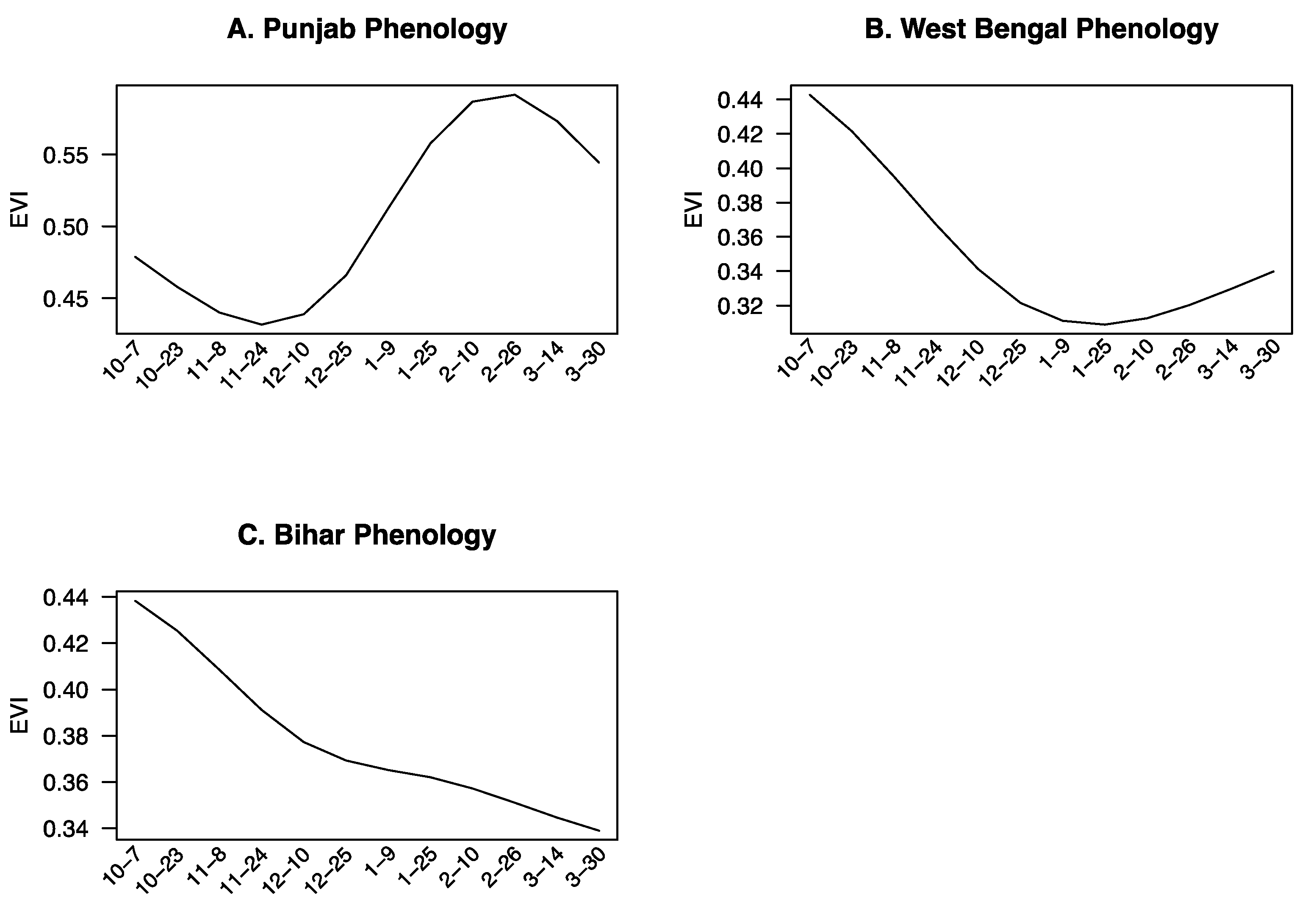
There are several reasons for this variation in accuracy based on location. First, in some regions (e.g., Southern and Eastern India), the MSA did not detect crop cover even though cropped area was visible in high-resolution imagery (e.g., Figure 3D,H; Table S2). One reason for this discrepancy is due to the timing of the MODIS EVI phenology that is associated with these pixels. For example, when examining the MODIS EVI phenology in pixels that appear to be cropped in high-resolution imagery in West Bengal, it appears as if the crop is planted earlier than the window defined as the winter growing season in our study (1 October to 31 March, Table S1), resulting in these pixels not being classified as cropped using the MSA (Figure 4B). It is likely that these fields are cropped with late monsoon or year-long crops, like horsegram or blackgram lentils, which continue to grow throughout the winter season, though they are planted during the previous monsoon season [26], and so are not defined as a winter crop in our method. In fact, the lowest R2 values occur in regions where the phenology used by the MSA does not match the phenology of crops seen in higher-resolution imagery (Table S1). When we restrict validation to only regions where phenology matched, we find individual regional R2 range between 0.45 and 0.89, and an overall R2 across all sites of 0.75. RMSE also decreases and ranges from 7.75 to 22.14 with an overall RMSE across all sites of 16.29. To examine the extent to which mismatches in phenology may be an issue with our MSA dataset, we used census statistics to calculate the percent of cropped area that is under all pulses and find that pulses comprise approximately 5% of winter cropped area across all districts and years [33]. A second reason for the discrepancy between high-resolution imagery and our MSA product is because our algorithm was unable to detect a peak in EVI phenology for pixels that are sparsely cropped, such as those sometimes found in regions like Bihar (Figure 4C). This outcome suggests that our MSA method may underestimate cropped area in regions with sparsely-cropped fields.
4.2. Additional Comparisons
When conducting high-resolution imagery validation for existing automated approaches to map cropped area using MODIS data, we find that accuracies across eight of our eleven high-resolution validation sites significantly decrease compared to our MSA validation results (Table S3). Validation values range between an R2 of 0.10 and 0.64 and an overall R2 of 0.44. RMSE values range from 19.41 to 40.40 with an overall RMSE of 30.08. This suggests that our MSA method is better able to capture sub-pixel heterogeneity resulting in higher accuracies compared to existing automated approaches that map cropped areas using MODIS satellite data.
We also examined the correlation between our MSA product and census statistics at the district scale using cropped area statistics provided by the Indian government from 2000–2001 to 2011–2012 [33]. Overall, R2 between our MSA product and census statistics across all states and years is 0.48. However, when we restrict validation to those states where we are confident that the phenology used in the MSA matches what is defined as winter crop in the census based on our high-resolution analysis (Table 1), overall R2 increases to 0.64.
Considering our regression analyses, we find that we are unable to detect a significant effect of increased irrigation on cropped area using census measures of cropped area, however, we are able to detect a significant effect of increased winter irrigation on winter cropped area using our MSA product for the districts considered in this study (Figure 1). This result suggests that our remote sensing product is better able to capture likely relationships between irrigation and cropped area compared to existing census statistics and our MSA product has the added benefit of producing data at a much higher spatial resolution of 1 × 1 km2 (Figure 5).
5. Discussion
We developed a new, automated method of mapping smallholder cropped area using MODIS satellite imagery that builds on previous approaches [11,15]. Our MSA method overcomes the three main challenges of mapping smallholder agriculture across large spatio-temporal scales because it: (1) accounts for sub-pixel heterogeneity by scaling the amount that a MODIS pixel is cropped between 0% and 100%; (2) is fully automated and does not require any data for calibration; and (3) can be used even in regions with high cloud cover due to the high overpass frequency of MODIS satellite imagery. Our method builds on existing approaches by accounting for sub-pixel heterogeneity typically associated with smallholder systems and requires no training data to translate peak EVI values to the percent that a pixel is cropped. When validated using high-resolution satellite imagery, this method results in R2 values that range between 0.19 and 0.89, and an overall R2 of 0.71 at a 1 × 1 km2 scale. Compared to existing census statistics, our product has the added benefit of producing high-resolution cropped area estimates that allow one to understand the factors influencing crop production at the sub-district scale (Figure 5).
The accuracies achieved in this study are similar to those found in other studies that use automated approaches to map crop production and do not use any calibration data [34,35,36]. Though our previous work found that accuracies can likely improve when using classified Landsat satellite data for calibration [11], it is not feasible to use this calibration method across large spatial and temporal scales in an automated way because the Landsat satellite data needed for calibration are not available in every region and in every year due to issues with cloud cover (Figure S1). Furthermore, classifying Landsat data into cropped versus non-cropped pixels requires ground data or visual inspection of high-resolution imagery which are often difficult to obtain across large spatio-temporal scales in smallholder systems [13]. This outcome suggests that depending on the scale of the study and the availability of calibration data, it may be worth using Landsat satellite data for calibration, as opposed to using the automated methods developed in this study. Despite the reduction in accuracy, however, we show that our automated approach that does not rely on any calibration data is still highly correlated with the cropped area seen in high-resolution imagery in eleven sites spread across India. Furthermore, these data were able to detect the association between winter irrigation and cropped area when including district fixed effects, suggesting that our remote sensing product can contribute to understanding the factors associated with variation in cropped area through time. Finally, our MSA method that scales peak EVI values was more accurate than previously used methods that only define a MODIS pixel as cropped or not cropped depending on whether it exhibits a peak in EVI phenology during the growing season (Table S3).
The accuracy of our method varied greatly based on the region under consideration suggesting some limitations of our approach. Our MSA cropped area estimates were most accurate in states like Punjab and Haryana (Table 1), where farming practices are more homogenous, a larger proportion of farms are cropped, and there are fewer sparsely-cropped pixels ([31]; Figure 3). Our MSA cropped area estimates were the least accurate in the states of West Bengal and Maharashtra (Table 1). There are several potential explanations for these discrepancies. First, there is likely a mismatch in the definition of winter crops between our cropped area algorithm and the cropped area seen in high-resolution imagery (Figure 3 and Figure 4). Second, our MSA product performed less well in regions where pixels were more sparsely cropped, as in the case of Gujarat and Bihar (Figure 3 and Figure 4). Our results suggest that our method may not be as accurate in regions with sparsely cropped fields, where approximately 10% or less of the MODIS pixel appears to be cropped based on high-resolution imagery. Finally, since peak EVI is influenced by yield and crop type, it is likely that our cropped area estimates performed less well and had increased error in regions that planted disparate crop types, had intercropped fields, and/or had fields with very different yields across space.
We have developed an R script that researchers can use to apply the MSA method to other areas with smallholder farms. Furthermore, in order to aid research on agricultural production at fine spatial scales in India, we are making our annual winter crop maps from 2000–2001 to 2015–2016 at 1 × 1 km2 produced in this study publically available. Both the data product as well as the R script will be distributed through the NASA Socioeconomic Data and Applications Center (SEDAC) hosted by the Center for International Earth Science Information Network (CIESIN) at Columbia University (http://sedac.ciesin.columbia.edu/).
Future work should consider how other products that have high temporal frequency but at a higher spatial resolution, such as Sentinel 2 and Planet Scope [37], may be used to map smallholder agriculture. It is likely that using this higher-resolution imagery will reduce inaccuracies in cropped area estimation caused by sub-pixel heterogeneity, as the resolution of this imagery (10 m and 5 m, respectively) better matches the size of individual smallholder fields. A second limitation of our study is that we were only able to validate our cropped area estimates using high-resolution imagery in eleven locations due to the unavailability of freely-available, high-resolution imagery across India. As higher resolution imagery becomes increasingly available across space and time (e.g., at a planetary scale), it would be beneficial to further validate our cropped area products to better understand the circumstances in which it has high (e.g., homogenous fields) versus low (e.g., sparsely cropped pixels) accuracies. Future work will also examine whether similar methods can be used to map cropped area during the monsoon season, when there is less data availability due to increased cloud cover and haze and it is more challenging to distinguish between cropped area and other natural or fallow vegetation that may green up due to monsoon rains.
6. Conclusions
This study developed a new automated approach, termed MSA, to map winter cropped area of smallholder farms using MODIS EVI data. We focus only on the winter (rabi) cropping season, and not the monsoon (kharif) season, as winter cropping is the main measure of cropping intensity in this region. While previous studies have successfully mapped cropped area of agriculture in regions with large field sizes, smallholder farms pose unique challenges given that (1) there is often a large amount of sub-pixel heterogeneity given the small field sizes and heterogeneous management across fields; (2) little to no calibration data exist to train algorithms; and (3) most smallholder farms are found in the tropics, where cloud cover may reduce image availability. This study evaluates an automated way to use satellite data to map a smallholder cropped area over large spatial and temporal scales, which is critical given that high-resolution production statistics rarely exist in smallholder systems. Our MSA method, which defines a pixel as cropped based on a hump-shaped phenology during the winter growing season and then scales the amount that this pixel is cropped between 0% and 100% based on peak EVI values, provides moderate to good accuracies when validated with high-resolution data (R2 ranging from 0.19 to 0.89 with an overall R2 of 0.71). Importantly, the MSA method requires no calibration data, making it easy to implement across large spatial and temporal scales. This method also results in 100% complete data coverage due to the availability of MODIS EVI data, even in years with high cloud cover. There are several limitations of our approach that should be examined in future studies. First, the accuracy of our method varied greatly based on region. Accuracies decreased when farming practices were more heterogeneous, a smaller proportion of farms were cropped, there were sparsely cropped MODIS pixels (defined as pixels that were <10% cropped), and where there was a mismatch in phenology between crops seen in high-resolution imagery and the timing used in the MSA window. Furthermore, since peak EVI is influenced by yield and crop type, it is likely that our cropped area estimates performed less well and had increased error in regions that planted disparate crop types, had intercropped fields, and/or had fields with very different yields across space. Second, our work focuses only on the winter cropping season and future work should examine whether our methods can also be applied to the monsoon season, when there is less data availability due to increased cloud cover and haze and it is more challenging to distinguish between cropped area and other natural or fallow vegetation that may green up due to monsoon rains. While we apply and evaluate the MSA only in India, we believe that this method can be used to map smallholder agriculture in other regions across the globe given that our method performed well in disparate agro-ecologies across India, which encompass a wide range in climates, crop types, crop management, and soils. In order to aid research on agricultural production at fine spatial scales in India, we are making the annual winter crop maps that we produce using the MSA from 2000–2001 to 2015–2016 at 1 × 1 km2 publically available through the NASA Socioeconomic Data and Applications Center (SEDAC) hosted by the Center for International Earth Science Information Network (CIESIN) at Columbia University (http://sedac.ciesin.columbia.edu/).
Supplementary Materials
The following are available online at www.mdpi.com/2072-4292/9/6/566/s1, Table S1: Timing of inflection points associated with start of the season green up dates for each of the eleven regions for which we have high-resolution data; Table S2: Confusion Matrix of cropped versus uncropped pixels in our cropped area product and high-resolution imagery; Table S3: R2 and RMSE values for eleven high-resolution validation sites when implementing the MODIS Peak method without scaling developed in previous studies; Figure S1: Available Landsat imagery from 2000–2001 to 2015–2016; Figure S2: Map of eleven high-resolution validation sites; Figure S3: Scatterplots of our MSA-derived estimates of cropped area versus high-resolution estimates of cropped area at a 1 × 1 km2 across eleven validation sites.
Acknowledgments
We thank Jaime Nickeson and colleagues at NASA’s NGA Commercial Data Archive Site (cad4nasa.gsfc.nasa.gov) for providing the necessary Quickbird and WorldView-2 imagery used in this study (Punjab, Gujarat, and West Bengal). We also thank Planet and their Ambassador’s program for making RapidEye and Planet Scope data available for this study [37]. This work was funded by a NASA Land Use and Land Cover Change (LCLUC) grant (NNX11AH98G) awarded to R.S.D., an NSF GRF and NASA New Investigator Award (NNH15ZDA001N) awarded to M.J., and a Google Earth Engine Research Award awarded to G.L.G.
Author Contributions
M.J., P.M., G.L.G., and R.S.D. conceived of and designed the study. M.J. and G.F. conducted the analyses in the study. M.J. wrote the initial draft of the manuscript, and all authors contributed to the final version.
Conflicts of Interest
The authors declare no conflict of interest. The founding sponsors had no role in the design of the study; in the collection, analyses, or interpretation of data; in the writing of the manuscript, and in the decision to publish the results.
References
- DeFries, R.; Mondal, P.; Singh, D.; Agrawal, I.; Fanzo, J.; Remans, R.; Wood, S. Synergies and trade-offs for sustainable agriculture: Nutritional yields and climate-resilience for cereal crops in Central India. Glob. Food Secur. 2016, 11, 44–53. [Google Scholar] [CrossRef]
- Fishman, R. More uneven distributions overturn benefits of higher precipitation for crop yields. Environ. Res. Lett. 2016, 11, 024004. [Google Scholar] [CrossRef]
- Lobell, D.B.; Schlenker, W.; Costa-Roberts, J. Climate trends and global crop production since 1980. Science 2011, 333, 616–620. [Google Scholar] [CrossRef] [PubMed]
- Godfray, H.C.J.; Beddington, J.R.; Crute, I.R.; Haddad, L.; Lawrence, D.; Muir, J.F.; Pretty, J.; Robinson, S.; Thomas, S.M.; Toulmin, C. Food security: The challenge of feeding 9 billion people. Science 2010, 327, 812–818. [Google Scholar] [CrossRef] [PubMed]
- Ray, D.K.; Ramankutty, N.; Mueller, N.D.; West, P.C.; Foley, J.A. Recent patterns of crop yield growth and stagnation. Nat. Commun. 2012, 3, 1293. [Google Scholar] [CrossRef] [PubMed]
- Shanahan, J.F.; Schepers, J.S.; Francis, D.D.; Varvel, G.E.; Wilhelm, W.W.; Tringe, J.M.; Schlemmer, M.R.; Major, D.J. Use of remote-sensing imagery to estimate corn grain yield. Agron. J. 2001, 93, 583–589. [Google Scholar] [CrossRef]
- Quarmby, N.A.; Milnes, M.; Hindle, T.L.; Silleos, N. The use of multi-temporal NDVI measurements from AVHRR data for crop yield estimation and prediction. Int. J. Remote Sens. 1993, 14, 199–210. [Google Scholar] [CrossRef]
- Doraiswamy, P.C.; Sinclair, T.R.; Hollinger, S.; Akhmedov, B.; Stern, A.; Prueger, J. Application of MODIS derived parameters for regional crop yield assessment. Remote Sens. Environ. 2005, 97, 192–202. [Google Scholar] [CrossRef]
- Wardlow, B.D.; Egbert, S.L. Large-area crop mapping using time-series MODIS 250 m NDVI data: An assessment for the U.S. Central Great Plains. Remote Sens. Environ. 2008, 112, 1096–1116. [Google Scholar] [CrossRef]
- Morton, J.F. The impact of climate change on smallholder and subsistence agriculture. Proc. Natl. Acad. Sci. USA 2007, 104, 19680–19685. [Google Scholar] [CrossRef] [PubMed]
- Jain, M.; Mondal, P.; DeFries, R.S.; Small, C.; Galford, G.L. Mapping cropping intensity of smallholder farms: A comparison of methods using multiple sensors. Remote Sens. Environ. 2013, 134, 210–213. [Google Scholar] [CrossRef]
- Jain, M.; Srivastava, A.K.; Balwinder-Singh; Joon, R.K.; McDonald, A.; Royal, K.; Lisaius, M.C.; Lobell, D.B. Mapping smallholder wheat yields and sowing dates using micro-satellite data. Remote Sens. 2016, 8, 860. [Google Scholar] [CrossRef]
- Carletto, C.; Jolliffe, D.; Banerjee, R. The Emperor Has No Data! Agricultural Statistics in Sub-Saharan Africa; World Bank Working Paper; World Bank: Washington, DC, USA, 2013; Available online: http://mortenjerven.com/wp-content/uploads/2013/04/Panel-3-Carletto.pdf (accessed on 7 January 2016).
- Whitcraft, A.K.; Vermote, E.F.; Becker-Reshef, I.; Justice, C.O. Cloud cover throughout the agricultural growing season: Impacts on passive optical earth observations. Remote Sens. Environ. 2015, 156, 438–447. [Google Scholar] [CrossRef]
- Biradar, C.M.; Xiao, X. Quantifying the area and spatial distribution of double-and triple-cropping croplands in India with multi-temporal MODIS imagery in 2005. Int. J. Remote Sens. 2011, 32, 367–386. [Google Scholar] [CrossRef]
- Spera, S.A.; Cohn, A.S.; VanWey, L.K. Recent cropping frequency, expansion, and abandonment in Mato Grosso, Brazil had selective land characteristics. Environ. Res. Lett. 2014, 9, 064010. [Google Scholar] [CrossRef]
- Lesk, C.; Rowhani, P.; Ramankutty, N. Influence of extreme weather disasters on global crop production. Nature 2016, 529, 84–87. [Google Scholar] [CrossRef] [PubMed]
- Gajbhiye, K.S.; Mandal, C. Agro-Ecological Zones, Their Soil Resource and Cropping Systems; National Bureau of Soil Survey and Land Use Planning: Nagpur, India, 2000; Available online: http://www.indiawaterportal.org/sites/indiawaterportal.org/files/01jan00sfm1.pdf (accessed on 11 December 2016).
- Chand, R.; Lakshmi Prasanna, P.A.; Singh, A. Farm size and productivity: Understanding the strengths of smallholders and improving their livelihoods. Econ. Political Wkly. 2011, 46, 5–11. [Google Scholar]
- Lobell, D.B.; Burke, M.B.; Tebaldi, C.; Mastrandrea, M.D.; Falcon, W.P.; Naylor, R.L. Prioritizing climate change adaptation needs for food security in 2030. Science 2008, 319, 607–610. [Google Scholar] [CrossRef] [PubMed]
- Mall, R.K.; Singh, R.; Gupta, A.; Srinivasan, G.; Rathore, L.S. Impact of climate change on Indian agriculture: A review. Clim. Chang. 2006, 78, 445–478. [Google Scholar] [CrossRef]
- Erenstein, O.; Thorpe, W. Livelihoods and agro-ecological gradients: A meso-level analysis in the Indo-Gangetic Plains, India. Agric. Syst. 2011, 104, 42–53. [Google Scholar] [CrossRef]
- Jain, M.; Naeem, S.; Orlove, B.; Modi, V.; DeFries, R.S. Understanding the causes and consequences of differential decision-making in adaptation research: Adapting to a delayed monsoon onset in Gujarat, India. Glob. Environ. Chang. 2015, 31, 98–109. [Google Scholar] [CrossRef]
- Wardlow, B.; Egbert, S.; Kastens, J. Analysis of time-series MODIS 250 m vegetation index data for crop classification in the U.S. Central Great Plains. Remote Sens. Environ. 2007, 108, 290–310. [Google Scholar] [CrossRef]
- Sakamoto, T.; Wardlow, B.D.; Gitelson, A.A.; Verma, S.B.; Suyker, A.E.; Arkebauer, T.J. A Two-step filtering approach for detecting maize and soybean phenology with time-series MODIS data. Remote Sens. Environ. 2010, 114, 2146–2159. [Google Scholar] [CrossRef]
- National Food Security Mission Crop Calendar of NFSM Crops. Available online: http://nfsm.gov.in/nfmis/RPT/CalenderReport.aspx (accessed on 10 January 2017).
- Xiao, X.; Boles, S.; Liu, J.; Zhuang, D.; Frolking, S.; Li, C.; Salas, W.; Moore, B., III. Mapping paddy rice agriculture in southern China using multi-temporal MODIS images. Remote Sens. Environ. 2005, 95, 480–492. [Google Scholar] [CrossRef]
- Ren, J.; Chen, Z.; Zhou, Q.; Tang, H. Regional yield estimation for winter wheat with MODIS-NDVI data in Shandong, China. Int. J. Appl. Earth Obs. Geoinf. 2008, 10, 403–413. [Google Scholar] [CrossRef]
- Becker-Reshef, I.; Vermote, E.; Lindeman, M.; Justice, C. A generalized regression-based model for forecasting winter wheat yields in Kansas and Ukraine using MODIS data. Remote Sens. Environ. 2010, 114, 1312–1323. [Google Scholar] [CrossRef]
- O’Brien, K.; Leichenko, R.; Kelkar, U.; Venema, H.; Aandahl, G.; Tompkins, H.; Javed, A.; Bhadwal, S.; Barg, S.; Nygaard, L.; et al. Mapping vulnerability to multiple stressors: Climate change and globalization in India. Glob. Environ. Chang. 2004, 14, 303–313. [Google Scholar] [CrossRef]
- Shah, T. Crop per drop of diesel? Energy squeeze on India’s smallholder irrigation. Econ. Political Wkly. 2007, 42, 4002–4009. [Google Scholar]
- Division, A.I. District Wise Land Use Statistics. Available online: http://aps.dac.gov.in/APY/Index.htm (accessed on 10 January 2017).
- Directorate of Economics and Statistics Area Production Yield Dataset-District 2016. Available online: http://aps.dac.gov.in/APY/Public_Report1.aspx (accessed on 1 September 2016).
- Duncan, J.M.A.; Dash, J.; Atkinson, P.M. Elucidating the impact of temperature variability and extremes on cereal croplands through remote sensing. Glob. Chang. Biol. 2014, 21, 1541–1551. [Google Scholar] [CrossRef] [PubMed]
- Xiao, X.; Boles, S.; Frolking, S.; Li, C.; Babu, J.Y.; Salas, W.; Moore, B., III. Mapping paddy rice agriculture in South and Southeast Asia using multi-temporal MODIS images. Remote Sens. Environ. 2006, 100, 95–113. [Google Scholar] [CrossRef]
- Lobell, D.B.; Thau, D.; Seifert, C.; Engle, E.; Little, B. A scalable satellite-based crop yield mapper. Remote Sens. Environ. 2015, 164, 324–333. [Google Scholar] [CrossRef]
- Planet Team. Planet Application Program Interface: In Space for Life on Earth. San Francisco, CA, 2017. Available online: https://api.planet.com (accessed on 1 February 2017).
Figure 1.
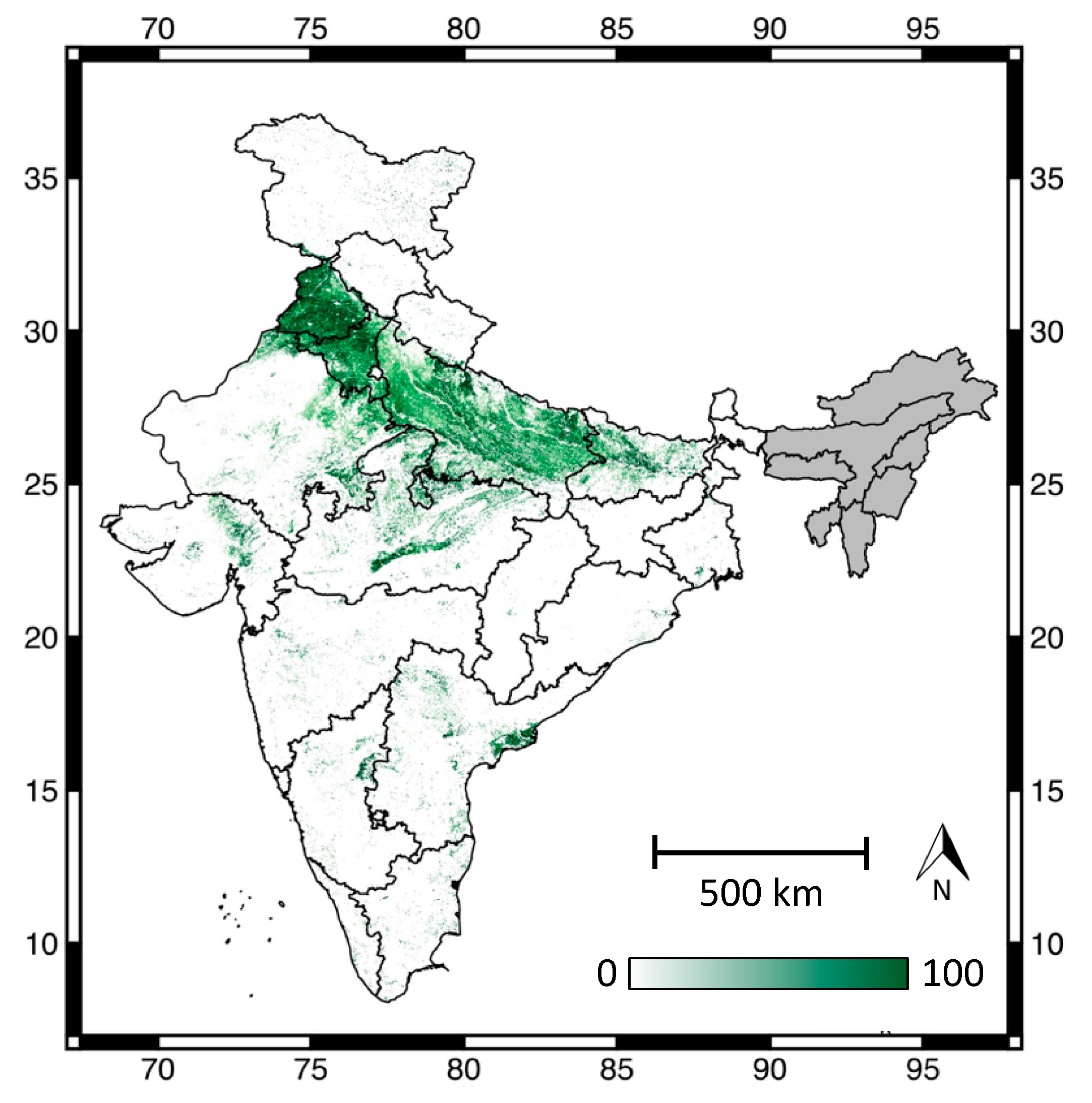
Study region is highlighted with the peak Enhanced Vegetation Index (EVI) from MODIS satellite data during the winter season growing season (1 October to 31 March) of 2001–2002. White represents pixels that did not exhibit a hump-shaped phenology and dark green represents high peak EVI values for pixels that exhibited a hump-shaped phenology after spline-smoothing the EVI time series. The northeastern states that were not considered in our study are highlighted in gray.
Figure 1.
Study region is highlighted with the peak Enhanced Vegetation Index (EVI) from MODIS satellite data during the winter season growing season (1 October to 31 March) of 2001–2002. White represents pixels that did not exhibit a hump-shaped phenology and dark green represents high peak EVI values for pixels that exhibited a hump-shaped phenology after spline-smoothing the EVI time series. The northeastern states that were not considered in our study are highlighted in gray.

Figure 2.
Example splined MODIS EVI phenology from Punjab, exhibiting characteristics of a cropped pixel as defined using MSA. Cropped pixels exhibit an increase in EVI representing green up after sowing (point 1) as well as a peak in EVI towards the end of the growing season due to crop senescence and harvest (point 2).
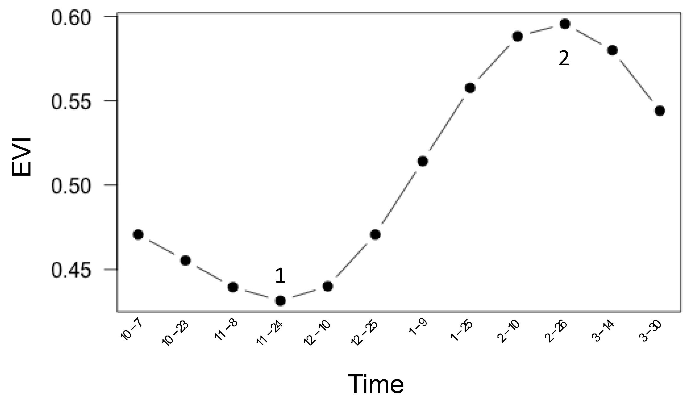
Figure 3.
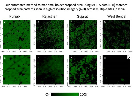
Cropped area as shown using high-resolution imagery (A–D) and cropped area estimates produced using the MSA (E–H) for Punjab (A,E), Rajasthan (B,F), Gujarat (C,G), and West Bengal (D,H). We selected these four sites to represent the range of validation accuracies from high (Punjab and Rajasthan), moderate (Gujarat), to low (West Bengal) R2 values. We find that overall cropped area patterns produced using the MSA match those seen in the high-resolution imagery, except for in the case of West Bengal. This lack of agreement is likely because the crops seen in the high-resolution imagery (D) were planted during the monsoon season, which occurs before the growing season window used by the MSA (H).
Figure 3.
Cropped area as shown using high-resolution imagery (A–D) and cropped area estimates produced using the MSA (E–H) for Punjab (A,E), Rajasthan (B,F), Gujarat (C,G), and West Bengal (D,H). We selected these four sites to represent the range of validation accuracies from high (Punjab and Rajasthan), moderate (Gujarat), to low (West Bengal) R2 values. We find that overall cropped area patterns produced using the MSA match those seen in the high-resolution imagery, except for in the case of West Bengal. This lack of agreement is likely because the crops seen in the high-resolution imagery (D) were planted during the monsoon season, which occurs before the growing season window used by the MSA (H).
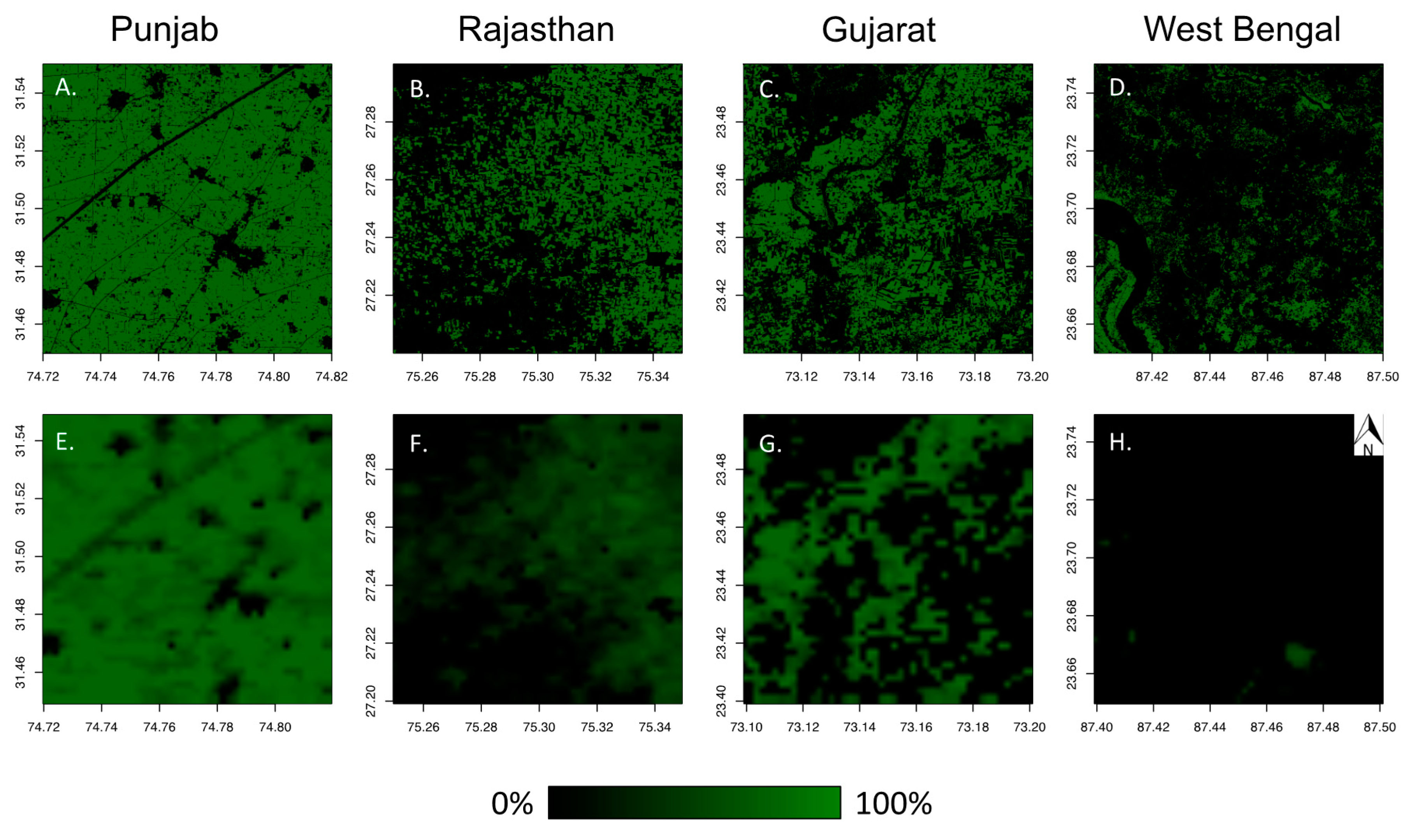
Figure 4.
Examples of MODIS EVI phenology for pixels that appear to be cropped in the high-resolution imagery for Punjab (A); West Bengal (B); and Bihar (C). The pixel from Punjab appears as cropped in our MSA dataset but the pixels from West Bengal and Bihar do not. In West Bengal, the crop was planted during the monsoon season (e.g., July to August) according to green up dates of the phenology and reached peak greenness before or very early in the winter growing season (e.g., September to October) considered in our study. The MSA method does not detect these pixels as cropped since the crop was planted during the monsoon season and does not green up during the winter growing season window. In Bihar, the pixel is very sparsely cropped, resulting in a slight green-up that is not counted as a peak in the MODIS EVI phenology by our MSA method. This result suggests that very sparsely-cropped pixels are not detected by our MSA algorithm.

Figure 5.
Cropped area map for 2000–2001 using our MSA derived product at a 1 × 1 km2 resolution. Non-cropped areas are highlighted in white and 100% cropped pixels are highlighted in dark green. States that were not considered in our study are shaded in gray.
Figure 5.
Cropped area map for 2000–2001 using our MSA derived product at a 1 × 1 km2 resolution. Non-cropped areas are highlighted in white and 100% cropped pixels are highlighted in dark green. States that were not considered in our study are shaded in gray.

Table 1.
Correlation values between our MSA product and estimates of cropped area using classified high-resolution imagery at 1 × 1 km2. The date and satellite for each high-resolution image and whether the winter-season window used in our MSA algorithm matched the MODIS EVI phenology of cropped pixels seen in the high-resolution imagery are also listed.
| Location | Image Date | Satellite | MSA R2 | MSA RMSE | Phenology Match |
|---|---|---|---|---|---|
| Rajasthan | 1-12-16 | RapidEye | 0.89 | 10.13 | Yes |
| Punjab | 1-31-11 | WorldView-2 | 0.78 | 7.75 | Yes |
| Uttar Pradesh 1 | 2-17-15 | RapidEye | 0.74 | 14.33 | Yes |
| Uttar Pradesh 2 | 2-15-15 | RapidEye | 0.72 | 13.18 | Yes |
| Bihar | 2-11-16 | SkySat | 0.73 | 22.14 | Yes |
| Haryana | 1-18-15 | RapidEye | 0.60 | 21.04 | Yes |
| Andhra Pradesh | 2-25-15 | RapidEye | 0.55 | 34.38 | No |
| Karnataka | 2-18-15 | RapidEye | 0.52 | 33.21 | No |
| Gujarat | 1-18-10 | WorldView-2 | 0.45 | 21.53 | Yes |
| Maharashtra | 2-17-15 | RapidEye | 0.41 | 30.02 | No |
| West Bengal | 1-12-08 | Quickbird | 0.19 | 27.87 | No |
| All 11 Sites | - | - | 0.71 | 18.47 | - |
| Sites with Phenology Match | - | - | 0.75 | 16.29 | - |
© 2017 by the authors. Licensee MDPI, Basel, Switzerland. This article is an open access article distributed under the terms and conditions of the Creative Commons Attribution (CC BY) license (http://creativecommons.org/licenses/by/4.0/).
Share and Cite
MDPI and ACS Style
Jain, M.; Mondal, P.; Galford, G.L.; Fiske, G.; DeFries, R.S. An Automated Approach to Map Winter Cropped Area of Smallholder Farms across Large Scales Using MODIS Imagery. Remote Sens. 2017, 9, 566. https://doi.org/10.3390/rs9060566
AMA Style
Jain M, Mondal P, Galford GL, Fiske G, DeFries RS. An Automated Approach to Map Winter Cropped Area of Smallholder Farms across Large Scales Using MODIS Imagery. Remote Sensing. 2017; 9(6):566. https://doi.org/10.3390/rs9060566
Chicago/Turabian StyleJain, Meha, Pinki Mondal, Gillian L. Galford, Greg Fiske, and Ruth S. DeFries. 2017. "An Automated Approach to Map Winter Cropped Area of Smallholder Farms across Large Scales Using MODIS Imagery" Remote Sensing 9, no. 6: 566. https://doi.org/10.3390/rs9060566
Note that from the first issue of 2016, this journal uses article numbers instead of page numbers. See further details here.