Detection of Oil near Shorelines during the Deepwater Horizon Oil Spill Using Synthetic Aperture Radar (SAR)

Abstract

During any marine oil spill, floating oil slicks that reach shorelines threaten a wide array of coastal habitats. To assess the presence of oil near shorelines during the Deepwater Horizon (DWH) oil spill, we scanned the library of Synthetic Aperture Radar (SAR) imagery collected during the event to determine which images intersected shorelines and appeared to contain oil. In total, 715 SAR images taken during the DWH spill were analyzed and processed, with 188 of the images clearly showing oil. Of these, 156 SAR images showed oil within 10 km of the shoreline with appropriate weather conditions for the detection of oil on SAR data. We found detectable oil in SAR images within 10 km of the shoreline from west Louisiana to west Florida, including near beaches, marshes, and islands. The high number of SAR images collected in Barataria Bay, Louisiana in 2010 allowed for the creation of a nearshore oiling persistence map. This analysis shows that, in some areas inside Barataria Bay, floating oil was detected on as many as 29 different days in 2010. The nearshore areas with persistent floating oil corresponded well with areas where ground survey crews discovered heavy shoreline oiling. We conclude that satellite-based SAR imagery can detect oil slicks near shorelines, even in sheltered areas. These data can help assess potential shoreline oil exposure without requiring boats or aircraft. This method can be particularly helpful when shoreline assessment crews are hampered by difficult access or, in the case of DWH, a particularly large spatial and temporal spill extent.

1. Introduction

The Gulf of Mexico has already experienced two of the largest oil spills in history, impacting both Mexican and US waters: the Ixtoc-1 and Deepwater Horizon (DWH) blowouts (in 1979 and 2010, respectively). The DWH event marked a new era in the application of satellite remote sensing and aerial surveillance for oil spill emergency response [1]. From April to August 2010, an extensive array of space-borne and aerial sensors were utilized to assess the evolution of the oil spill on a daily basis. Due to the length of this event (87 days), it was the first time incident responders and scientists were able to capture the same event from an entire suite of remote sensing platforms and sensors, including Synthetic Aperture Radar (SAR) and optical detectors operating in the thermal and visible bands, some with multispectral or hyperspectral sensors. The quantity of data collected during DWH allows for new advances in remote sensing algorithms and new applications for remote sensing in oil spill response.

During the DWH event, oil contamination was evident along the U.S. coastal areas [2]. Both during and after the spill, natural resource trustees along the Gulf Coast attempted to identify DWH oil along the shoreline, on the ground, as well as from boats, airplanes, and space-borne satellites, including SAR satellites. SAR is well known for its capability to detect oil spills [3], oil from natural seepage or maritime transit (vessels and other structures, e.g., platforms), and other oceanographic and atmospheric processes [4]. Radar offers a number of advantages over other sensors/wavelengths for recognizing and monitoring oil in the ocean. Contrary to passive optical imaging systems that require solar illumination (and are limited by cloud coverage), SAR and other imaging radar systems utilize their own active illumination systems [5]. Thus, SAR supports earth monitoring activities that are less constrained by weather and sun illumination conditions [6,7], but can be constrained by adverse rain and wind conditions, as will be discussed.

In a spill such as DWH where hundreds of miles of marsh shorelines are exposed to oil, spill responders cannot feasibly assess all potentially exposed shoreline areas. Similarly, when the spill lasts for multiple months, spill responders are unlikely to be able to assess all of the oil that comes ashore. In these situations, satellite-based remote sensing data can play an important role as a supplement to shoreline monitoring. For this paper, we investigated the limits and merits of multiple satellite SAR platforms available in 2010, as well as multiple beam mode configurations. If another major oil spill were to occur along a marsh coastline in the future, the work presented here could be used to determine appropriate SAR acquisition settings, including optimal resolution, beam mode, and incidence angles.

Multiple remote sensing studies have been carried out with the objective of observing oil on the near coastal environments. Ramsey et al. [8] used full polarimetric SAR collected by UAVSAR to map the occurrence along shorelines and showed the possibility of oil penetrating past the shoreline into the back marsh. Kokaly et al. [9] and Khanna et al. [10] used spectroscopic and aerial remote sensing data from three Airborne Visible/Infrared Imaging Spectrometer (AVIRIS) datasets on a particular region inside the Barataria Bay marshes to detect oil inside the canopies on the marshes. These studies found that scaling their observations to a coarser satellite-based spatial sensor (Landsat Enhanced Thematic Mapper Plus, or ETM+) greatly reduced the detection of oil spectral signatures. After the DWH spill, Ramsey et al. [11] carried out a multiyear monitoring study using the aerial UAVSAR sensor over the marsh sites affected by the DWH on the Barataria Bay. This study demonstrated the utility of radar-based oil detection in marsh habitats, but the data collection included the logistical challenge and expense of mobilization aircraft. The continued challenges of assessing oil transport and deposition in marsh habitats provides context for the importance of monitoring oil both as it approaches and after it reaches the shoreline. For this study, we considered satellite SAR data collected during DWH as an opportunity to use satellite-based SAR technology as a tool for assessing oil fate and transport in nearshore environments.

Satellite SAR has rarely been used to detect oil near shorelines, but has been used extensively to detect oil in open water. Garcia-Pineda et al. [7] developed a semi-automated SAR oil delineation algorithm called the Textural Classifier Neural Network Algorithm (TCNNA). Garcia-Pineda et al. [12,13] further refined the algorithm to process SAR imagery collected during the DWH event to identify not only presence/absence of oil, but to identify oil emulsions that are detectable in SAR imagery. TCNNA is semi-automated because it can still be subject to false positive oil detections; thus, the final delineation of oil in SAR imagery requires a detailed inspection from a trained SAR image interpreter.

For many years, satellite SAR was considered to be a tool for detecting oil in open ocean environments [14,15]; oil in nearshore marsh habitats was evaluated mostly from the ground or low-flying aircraft [2,3,16] or from aerial SAR platforms such as UAVSAR [8,11]. However, during DWH, oil was detectable in satellite SAR imagery in Louisiana nearshore areas, including areas with marsh habitats, on the vast majority of days during the DWH spill.

In this paper, we present a novel method of quantifying oil exposure in nearshore habitat using only satellite-based SAR imagery. Specifically, we focus on the processing and TCNNA analysis of satellite SAR data collected during the DWH event, allowing us to quantify the spatial and temporal extent of oil approaching the shoreline in Louisiana. We address the issues that have previously hampered the use of satellite SAR in nearshore areas and present satellite SAR data that suggest a correlation between the temporal extent of detectable oil near shorelines and the amount of oil that Shoreline Cleanup and Assessment Technique (SCAT) crews recorded [17]. Because of the wealth of satellite SAR imagery collected during the DWH spill, we were able to address questions such as whether satellite SAR imagery is useful for detecting oil in or near marsh habitats, and whether daily SAR imagery can provide insights into potential nearshore oil exposure from a multi-month spill such as DWH.

To encourage ongoing and collaborative research, the classified oil outputs (TCNNA algorithm products) from the SAR imagery described in this manuscript are publically available through the NOAA Office of Response and Restoration on the Environmental Response Management Application (ERMA) [18].

2. Materials and Methods

2.1. SAR Overview

SAR satellites comprise active microwave high-spatial resolution sensors that operate across a range of frequencies including X-band (8–12 GHz, 2.5–4 cm), C-band (4–8 GHz, 4–8 cm) and L-band (1–2 GHz, 15–30 cm). As an active sensor, SAR’s transmitted electromagnetic field is controlled for amplitude, phase, and polarization. These characteristics are also measured for the received field, which, after proper coherent processing of the raw signal, yields a high-spatial resolution complex reflectivity map of the observed scene [19].

Image amplitude is a response to the microwave signal backscattering properties of the ocean surface. The backscatter measured by a SAR sensor is a function of radar incidence angle, which is the angle between the incident radar beam and the vertical intercepting surface. For ocean imaging, the energy detected by the SAR antenna shows a stronger influence of Radar Cross Section (RCS). The RCS is a measure of the power scattered in a given direction when a target is illuminated by an incident electromagnetic wave [20]. The RCS is normalized to the power density of the incident wave at the target so that it does not depend on the distance of the target from the illumination source. As the energy incident angle increases (with respect to nadir), the RCS also increases and less energy per unit area is reflected back to the satellite [5]. This effect produces SAR ocean images with a gradient of decreasing brightness from the near-nadir to the far-nadir sides of the image [8].

An image of the sea surface typically shows local variation in roughness, which is a function of wind waves and swell. Surface oil modulates the fine-scale roughness and enhances specular reflection from the sea water surface under the oil. This results in a signal that is locally less intense than from the surrounding oil-free water, thus making the oil slick in SAR imagery appear darker than water [7,21]. When the sea surface roughness is dampened or smoothed by viscoelastic properties of an oil slick or any other surfactant, incident energy from the SAR spacecraft is reflected away from the sensor, reducing radar backscatter. 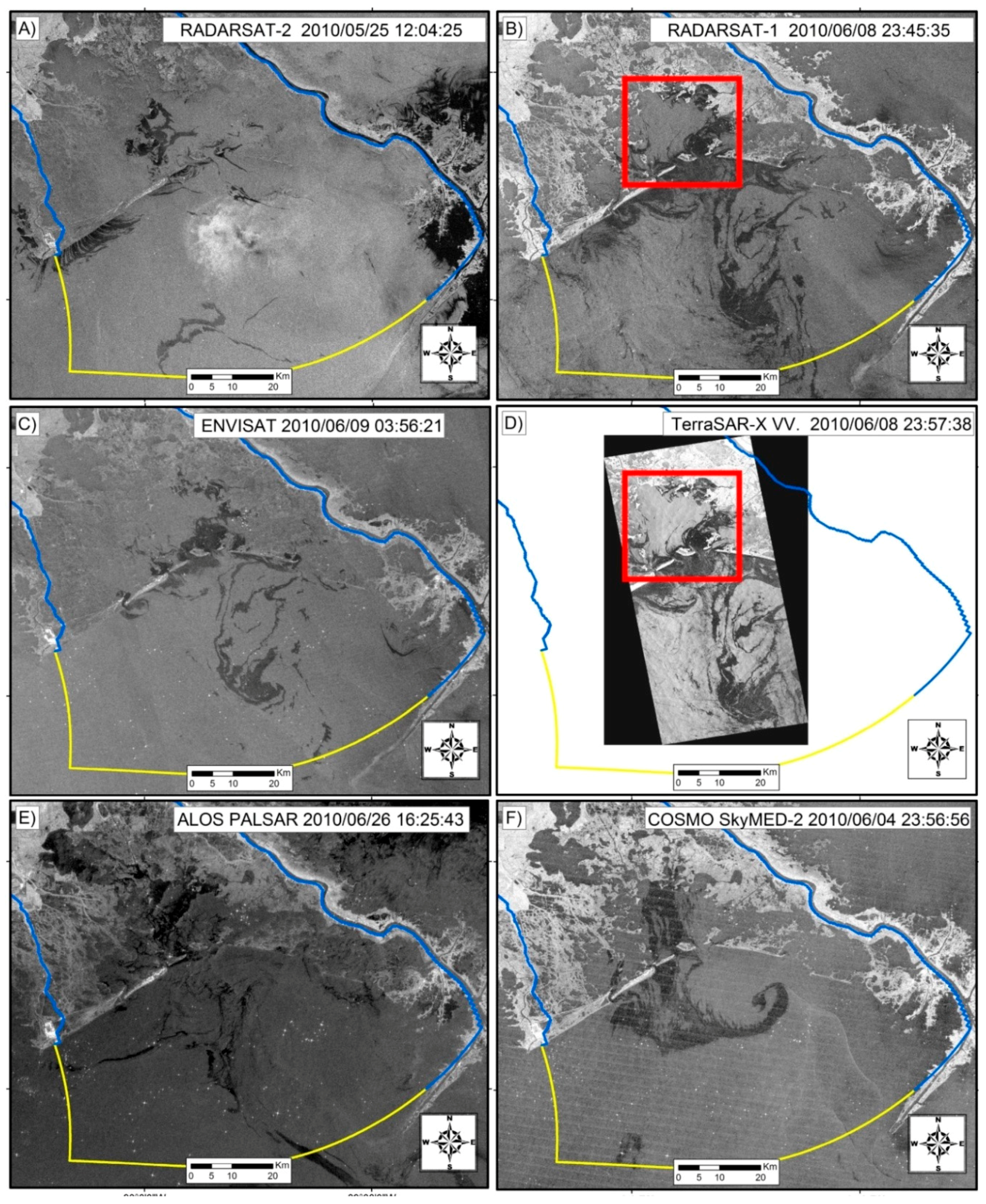Therefore, oil-covered areas usually have distinctly contrasting brightness against the radar backscatter produced by wind-generated ripples [6]. The visual differences among the satellites images (Figure 1) are based on the specific configuration of the satellites including: wavelengths, spatial resolution, incidence angle, specific weather conditions present at the moment of the SAR snapshot, and the instrument noise floor.

The example images in Figure 1 cover the west side of the Mississippi River “bird’s foot” peninsula and the Barataria Bay region of the central Louisiana coast. In all of the examples, floating oil (dark areas on the imagery) is present inside and outside of the bay. Because of geometry factors (commonly known as a double bounce effect of the backscatter), land areas are very bright features on SAR imagery, although this brightness can be more or less contrasting depending on the beam angles and wavelengths.

Figure 1 illustrates some of the differences and similarities observed by SAR sensors. The area covered in the six images is approximately the same, but the data vary by sensor. The primary differences are frequencies, pixel resolution, incidence angles, and noise floor. We note that three of the satellites used during DWH—Envisat (Figure 1C), RADARSAT-1 (Figure 1B), and ALOS-1 (Figure 1E)—are no longer operational. However, all three satellites have been or are currently being replaced by successor instruments (SENTINEL-1, RADARSAT-2, and ALOS-2, respectively).

On the satellites, the antenna for a SAR system is designed so that the transmitted and received radar waves are vertically (V) or horizontally (H) polarized. In marine applications, the most appropriate single-polarimetric SAR mode is VV; the first V indicates transmission of an electromagnetic field temporally oscillating along a vertical plane relative to the SAR antenna, and the second V indicates vertical received polarization [3]. Current SAR systems have polarimetric diversity, including several unique sets of polarimetric modes. Single-polarization is no longer limited to co-polarized images; a cross-polarized image such as VH or HV can now be obtained. In dual-polarimetric mode, one (or two) linear polarization(s) is transmitted and two (or one) linear polarization(s) are received, resulting in three optional pairs of co- and cross-polarized images: HH and HV, VV and HV, or HH and VV. Finally, in the full-polarimetric mode, the SAR antenna transmits and receives vertically and horizontally polarized electromagnetic fields so that a full scattering matrix can be measured, resulting in HH, VV, HV and VH images. This mode is usually referred to as quad polarization (or “Quad Pol”) and is available on RADARSAT-2 [19] and ALOS-2.

Detection of an oil slick will vary depending on the sensor wavelength and configuration. For example, a short wavelength X-band (Figure 1D,F) is more sensitive to smaller variations on the surface geometry and generally produces a higher contrast between floating oil and the surrounding clean water. However, X-band imagery can contain a considerable amount of speckle noise. In contrast, a longer wavelength L-band (Figure 1E) introduces less weather factor noise (e.g., rain cells) on the imagery by increasing the size of the sampling frequency. Because of the longer wavelength, the image is smoother and shows less speckle.

At the time of this writing, the satellite with the best signal-to-noise ratio is RADARSAT-2 (Figure 1A). COSMO-SkyMed satellites, on the other hand, typically include antenna patterns that incorporate significant noise on the imagery (Figure 1F). The satellite with the highest spatial resolution used during the DWH event was TerraSAR-X (Figure 1D), with a resampled spatial pixel resolution of approximately 2.3 m. All of the SAR satellites are capable of aiming at different areas within the range of the viewing angles, and expanding or contracting the area covered, which results in a corresponding decrease or increase of the spatial resolution. For example, the high resolution in TerraSAR-X (Figure 1D) allows for the capture of the fine detail features of floating oil, but reduces the areal extent of the image footprint to only 32 km wide. In contrast, for images collected during DWH, the approximate resolution of the resampled pixel size for RADARSAT-2 was 25 m (ten times more than TerraSAR-X), while COSMO-SkyMed’s ScanSAR resolution was 30 m. The image swath of these two satellites was approximately 300 and 200 km, respectively.

When using SAR to detect oil in proximity to coastal areas, sensor parameters such as noise floor, spatial resolution, polarimetry, and viewing angles are crucial factors on the ability to discern oil from other look-alikes. 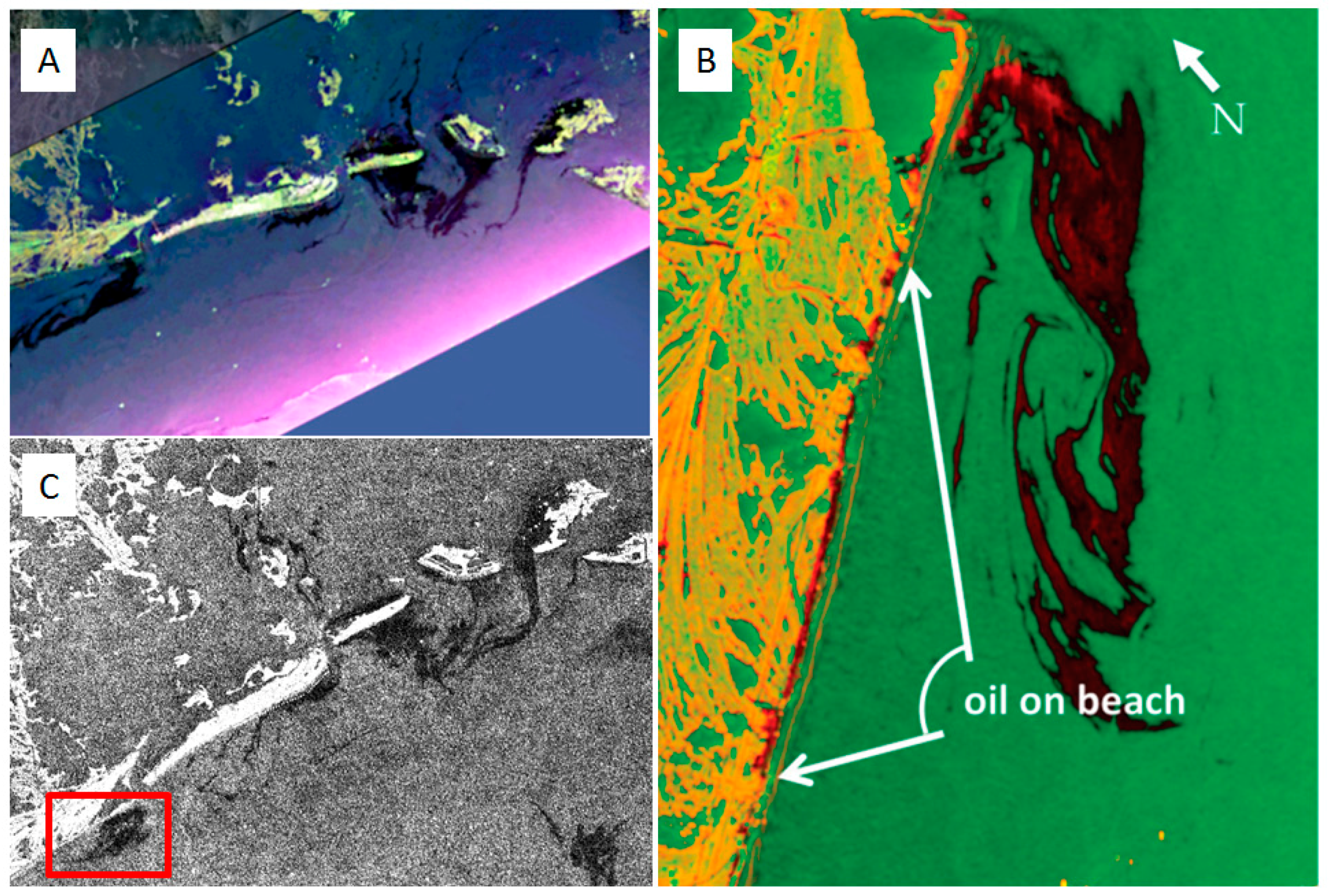Since oil slicks produce a specular reflector of the sea surface, the noise floor of the SAR sensor limits the distinction of the oil from other features when there is lack of gravity or capillary waves generated by wind [7]. The conditions needed for the detection of oil in SAR imagery in proximity to the shoreline are a function of the signal to noise ratio, which is often driven by the noise floor of the SAR sensor. At the time of this writing, the SAR sensor with the highest resolution, noise floor, and signal to noise ratio is UAVSAR (Figure 2A). This L-Band SAR sensor is mounted on an airplane and was used during the DWH to identify oil in proximity to the nearshore environment [22]. UAVSAR typically collects SAR data with quad polarization, which allows a more advance processing by obtaining the phase among polarizations and therefore the capability to apply multiple post-processing algorithms. The research and development of UAVSAR at JPL-NASA has application to satellite-based SAR sensors as well. For example, Minchew et al. [23,24] detected oil emulsion mixtures using UAVSAR. Garcia-Pineda et al. [13] applied a similar analysis to SAR satellite data to detect emulsified oil on the ocean surface.

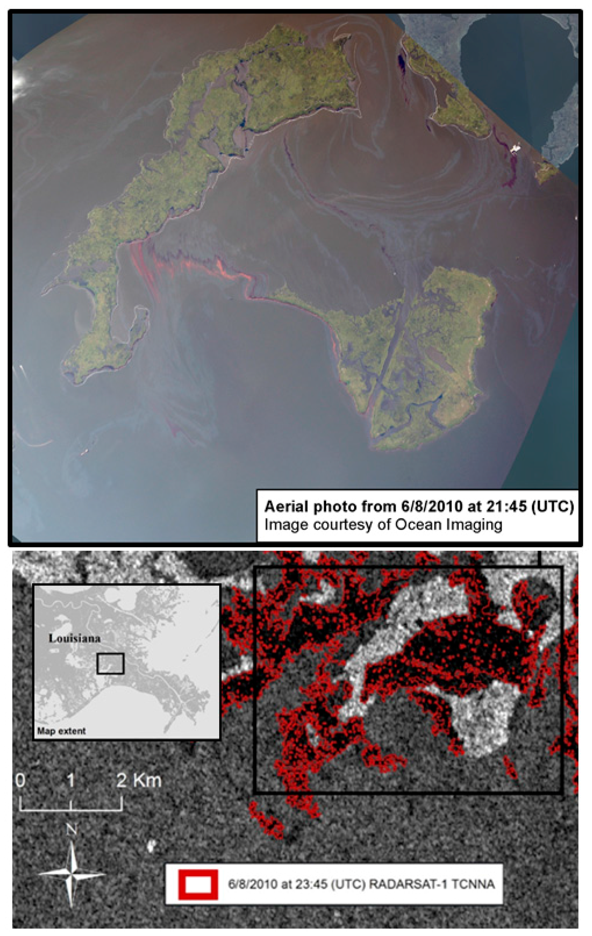
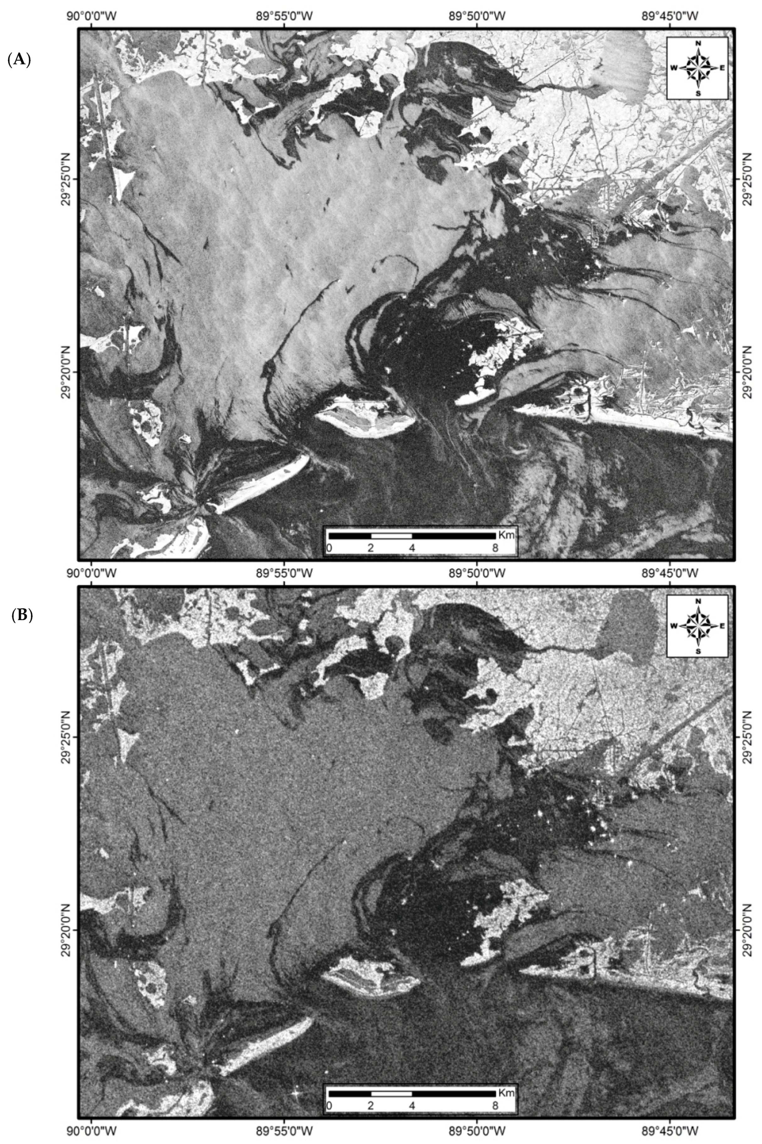
The example shown in Figure 2 is a sequence of UAVSAR collected on 23 June 2010 (Figure 2A) followed by RADARSAT-1 (Figure 2C) collected over the same area on two days after on June 25. Figure 2B corresponds to the same area covered by the red outline inside Figure 2C. Jones et al. [22] originally presented this UAVSAR subscene to demonstrate the ability of aerial UAVSAR to detect oil near the shoreline. The image on Figure 2B is showing the averaged intensity (green) and entropy (red) from the Cloude-Pottier polarimetric decomposition in the vicinity of Elmer’s Island, Louisiana, immediately southwest of the barrier islands shown in Figure 2B. Oil can be seen along the beaches of the island while a large oil mass approaches the shore. This sequence shown by Figure 2A,B suggests that oil persisted in the nearshore environment for more than 36 h.

2.2. SAR Image Processing

Numerous SAR satellites collected imagery from the northern Gulf of Mexico during the DWH spill. We obtained 710 SAR images collected between 23 April and 12 August 2010, each covering an area in the northern Gulf of Mexico where oil was detectable at some point during the spill. To analyze for the presence of oil near the shoreline, we initially identified 292 SAR images that appeared to contain oil within 25 km of a shoreline. Based on previous studies that described the optimal weather conditions for detecting oil in SAR imagery [7,12], we selected a subset of 188 images with weather-compliant conditions (winds from 3–8 m/s) and appeared to contain floating oil from the DWH. The SAR imagery used in this analysis was collected by RADARSAT-1, RADARSAT-2, TerraSAR-X, COSMO-SkyMed 1-2-3-4, Envisat, ALOS-1, and ERS-2 satellites (

Table 1. SAR data available for analysis.

Band	Satellite	Number of Images on Dataset	Operating Incidence Angles	Frames Selected for Analysis
C-Band	RADARSAT-1	67	20–50	31
	RADARSAT-2	129	20–50	26
	Envisat	97	15–45	34
	ERS-2	37	20–26	3
X-Band	COSMO-SkyMed	231	20–59	49
	TerraSAR-X	74	20–45	8
L-Band	ALOS-1	75	18–43	5
	Total	710		188

).

Data were obtained in a wide range of formats including N1 (Envisat), Level1-SIO, GeoTIFF 8 bit, and GeoTIFF 16 bit. Based on the format of the SAR data available, we used four different remote sensing analysis tools to inspect the imagery on its highest available radiometric resolution: Matlab Imaging-Mapping Toolbox, IDL Image Library, MapReady, and ESRI ArcMap.

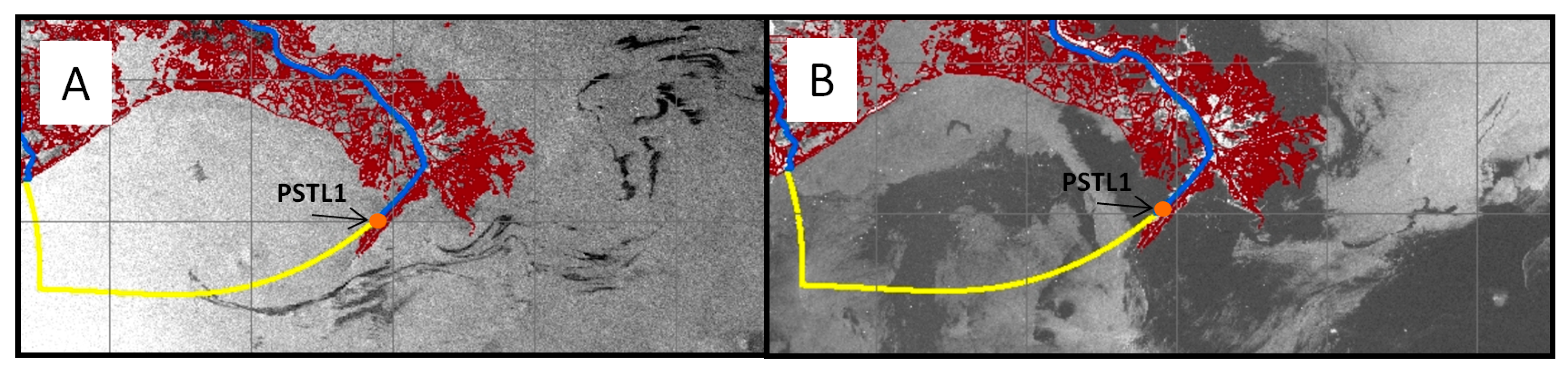
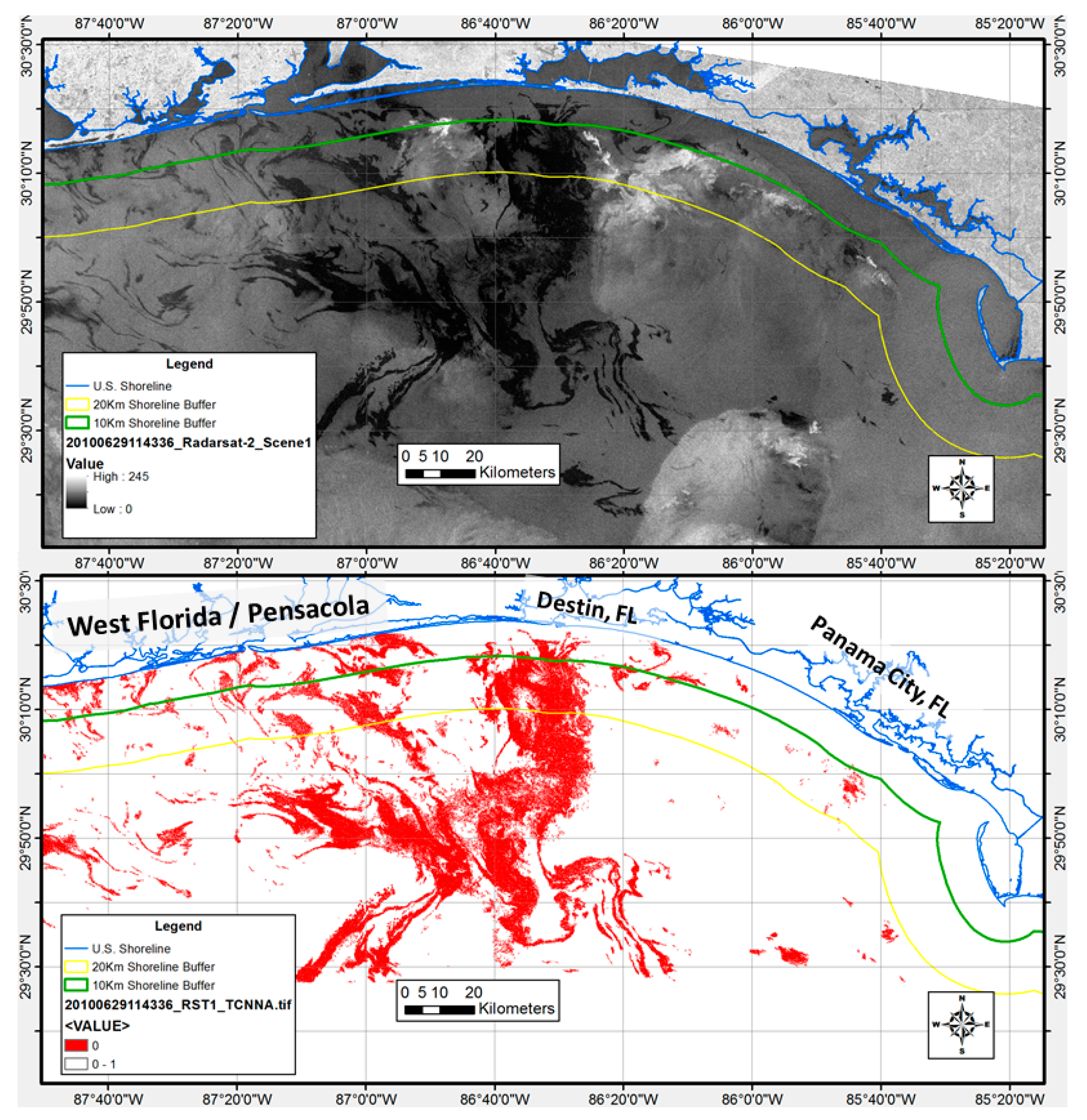
We inspected the entire catalog of 710 images, which included images collected over a wide range of weather conditions. Figure 3A shows a sub-scene from a SAR image collected by RADARSAT-2 on 21 July 2010 at 23:52 UTC. On this SAR snapshot, oil is detectable within 1 km of the shoreline of the Mississippi delta when Station PSTL1 from the NOAA National Data Buoy Center (NDBC) registered a wind speed 9.4 m/s with gusts above 10 m/s. As reported by Garcia-Pineda et al. [12], DWH oil was observed on SAR images even at winds of 20 m/s in the open water during storm events. The strong winds and the intense turbulence of the surface water that prevailed for several hours were unable to dissipate the massive amount of floating oil. On the other hand, unfavorable weather conditions for oil-water discrimination were commonly observed. Figure 3B shows a SAR sub-scene collected by RADARSAT-2 on 1 June 2010, at 12:01 UTC. In this case, low wind conditions prevailed for several hours; the Station PSTL1 registered 1.6 m/s at the time of the SAR snapshot. In such low-wind conditions, oil is usually not discernable. For this study, such images were discarded.

For this study, we discarded nearly 75% of the DWH imagery for a variety of reasons, including in particular when meteorological conditions interfered with the ability to detect oil. Particularly during the summer, the sea surface temperature of the GOM favors the formation of storms. Floating oil is difficult and sometimes impossible to be delineated under rain cells or turbulent waters generated by fronts or tropical storms. 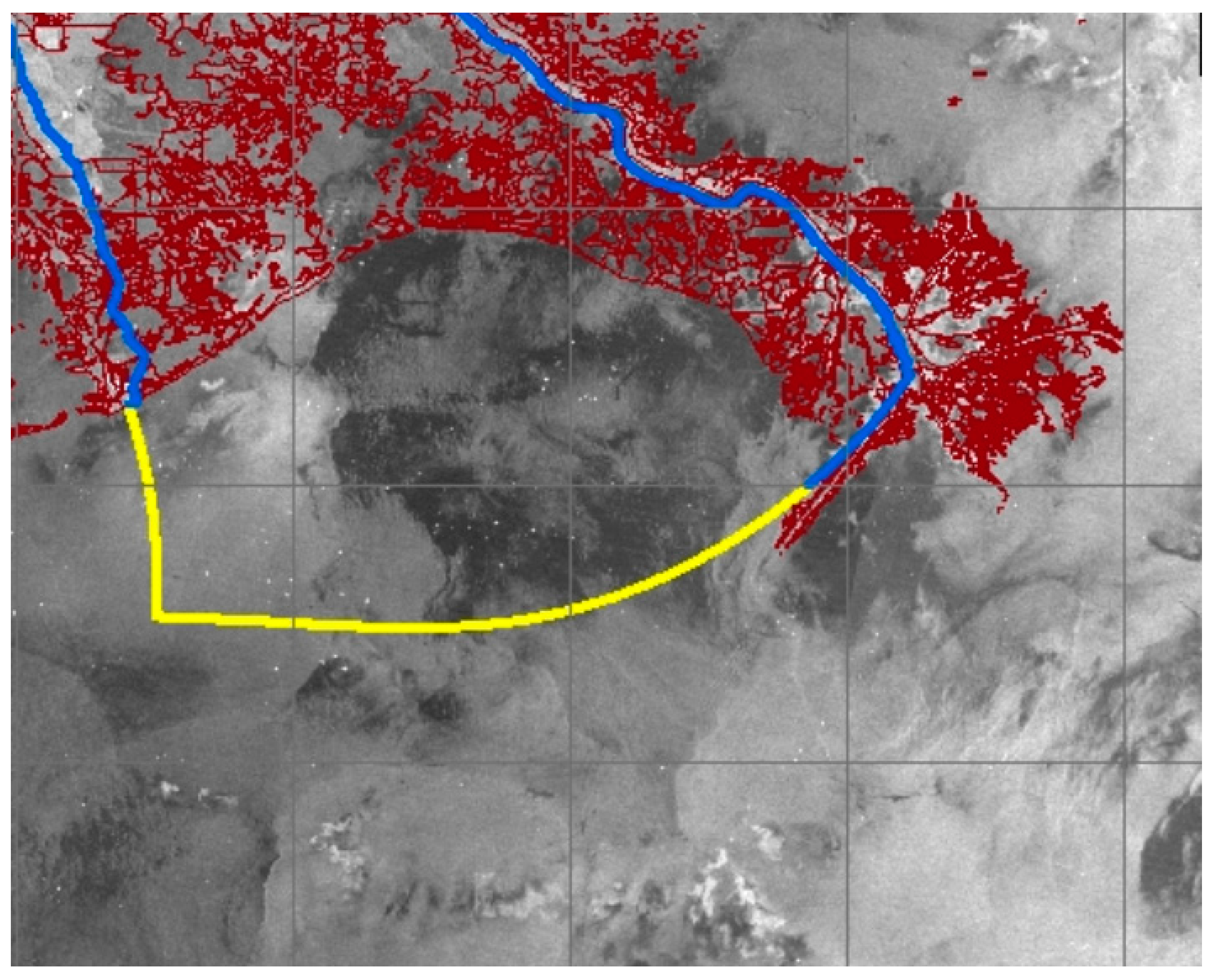Figure 4 shows an example of stormy weather that complicates the delineation of oil. Mesoscale storms on the open water usually generate an imbalance of the wind, producing rain cells and pockets of strong winds (which mask the surface oil) with nearby areas of low wind (where oil slicks cannot be discerned). The operating minimum wind threshold for the TCNNA algorithm is above 2 m/s [12]; SAR images outside this weather condition (e.g., dark areas of Figure 4) were not included in this analysis.

The 188 selected images were processed for segmentation of floating oil using the TCNNA. This algorithm utilizes input data in GeoTIFF format, rescaling the radiometric resolution within a pixel range. Therefore, the selected imagery was converted to 16-bit GeoTIFF format, or we used 8-bit GeoTIFF format when raw SAR data was not available. The TCNNA semi-automated routine filters a grayscale image with a variable boundary kernel size (typically a 25 × 25 pixel kernel or larger, depending on the spatial resolution) for edge and shape detections based upon the Leung-Malik filter bank [7,12]. The neural network algorithm interpolates these detections within a training set previously compiled by an expert operator through classification of several thousand pixels from the same images under analysis.

SAR detection of oil on the sea surface relies on the damping effect of the oil on the Bragg waves. However, the observed reduced radar backscatter on the sea surface is not unique to oil. Low winds, biogenic films, wind sheltering by land or submerged structures, grease ice, internal waves, ship wakes, and convergence zones can also create areas of reduced radar backscatter [19]. In addition, thunderstorms, rain, as well as atmospheric and oceanic fronts can affect the surface roughness and produce so-called “look-alike” features (Figure 5). Furthermore, oil on the sea surface is subjected to a number of processes including evaporation, dispersion, emulsification, dissolution, oxidation, sedimentation, and biodegradation. For these reasons, the detectability of oil with SAR is sensitive to the source of the oil, the current environmental conditions, and the history of the sea surface in localized areas [12,13].

In this study, a supervised evaluation of each image was required to identify and remove image regions unsuitable for analysis. SAR images cover large areas (in some cases swaths 450 km wide) and weather conditions vary on regional scales. Although all of the images used in this analysis clearly showed the presence of floating oil, in some cases portions of SAR images were obscured due to sensor noise or other issues with the raw image data. Under local conditions of low or zero wind, substantial regions of an image would sometimes appear radar-dark in the absence of capillary waves on the ocean surface. In some images, regions of noise or low wind were masked off from the surrounding image features to avoid false-positive classifications; these areas were classified as no-data regions on the image. Screening filters (land masks) were used to prevent false positive oil detections on land.

Since the neural network classifier operates on a per-pixel basis, the TCNNA output maintains the original spatial resolution of the SAR image. The fully implemented TCNNA routine produces a ~1 Mbyte georeferenced raster image in which all pixels have a binary classification of either floating oil or not floating oil. Resolution of individual pixels depended upon the satellite, collection mode, and incidence angle, but was generally in the range of 12.5 to 75 m. These images with binary classifications were produced in GeoTIFF format, preserving the projection and datum of the input SAR image (e.g., UTM and NAD83). TCNNA GeoTIFF outputs were then converted to ESRI ArcMap shapefiles and if necessary re-projected to the NAD83 datum to standardize all the outputs. The resulting TCNNA shapefiles were then inspected for false positives.

2.3. Identification and Removal of False Positives

For the false positive inspection, we first overlaid North American Mesoscale (NAM) wind model outputs on the TCNNA and SAR images layers in GIS for visual inspection. Additionally, we used direct wind and atmospheric measurements from the nearest weather and buoy stations from the NDBC. The SAR image and TCNNA-detected oil areas were then inspected for features (dark patches on the SAR images) that might have been created by areas with wind speeds <2 m/s.

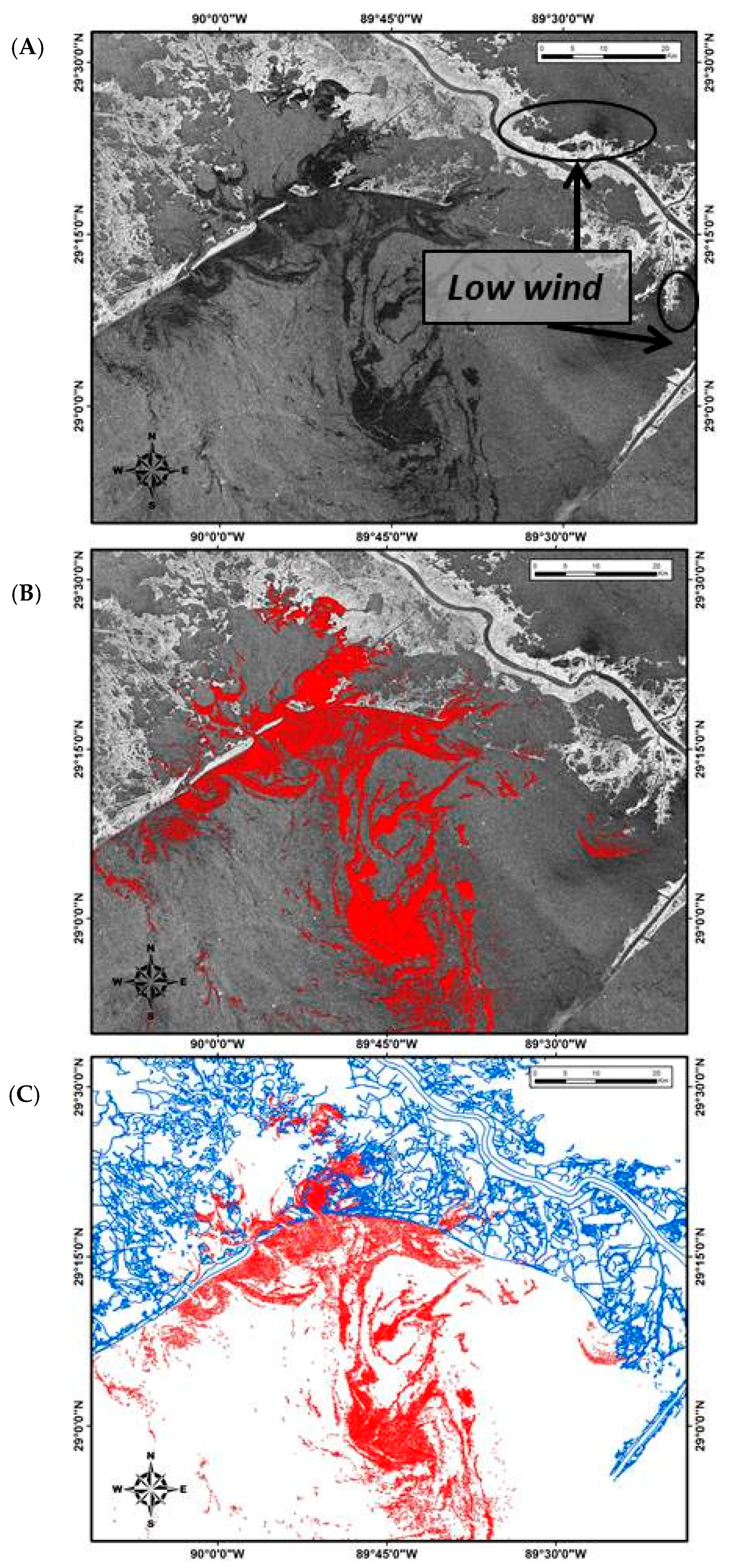
Although the NAM wind model outputs and NDBC data were useful reference data for identifying potential low wind areas, these data sets were typically at much lower resolution than the underlying SAR image. Thus, low wind features (false positives) had to be identified in a supervised classification based on the additional lines of evidence, including texture and proximity to land (Figure 5). In particular, low backscatter signatures can be generated when land obstructs the flow of the wind required to generate capillary waves on the sea surface. A trained image analyst can identify these features by looking at the gradient of the pixel values at the edge of the dark feature. Normally, floating oil will have a higher contrast between the edge of the slick and the surrounding waters (Figure 5A). The TCNNA algorithm will normally flag low wind features, and the analyst has the option of removing all or some of the flagged pixels [7,12]. The algorithm uses the statistical descriptors of the neighbor pixels under analysis in search for variances on the strength of the backscatter. Although the algorithm flags the majority of the low wind features, some areas require the analyst to inspect the output for quality assurance. Most of these cases occur on areas shadowed by land or behind islands. In these areas, we used a high resolution land mask [25] to remove low backscatter features created by land.

When low wind regions were indicated by low modelled wind in the NAM, observations from buoys and weather stations, and confirmed in the TCNNA outputs, these regions were manually removed from the original TCNNA output. In cases where large low wind regions were intermixed with the oil area and boundary-specific demarcation between oil and low wind was difficult, the entire SAR image was discarded from the analysis.

Other features can generate false positives in addition to low wind. For example, rain cells often generate regions of low backscatter (particularly on shorter wavelength X-Band). Low altitude barrier islands or very shallow marshes may also create low backscatter on the SAR image (especially on longer wavelength L-Band). The supervised classification step included close inspection of TCNNA output to ensure that these common false positives were not present.

Figure 5A–C shows the flow of the SAR data analysis: (Figure 5A) general visual inspection of the SAR imagery; (Figure 5B) overlay of the TCNNA output for removal of low wind features; and (Figure 5C) overlay of the high resolution land and bathymetry layer for land masking and removal of low backscatter caused by land obstruction.

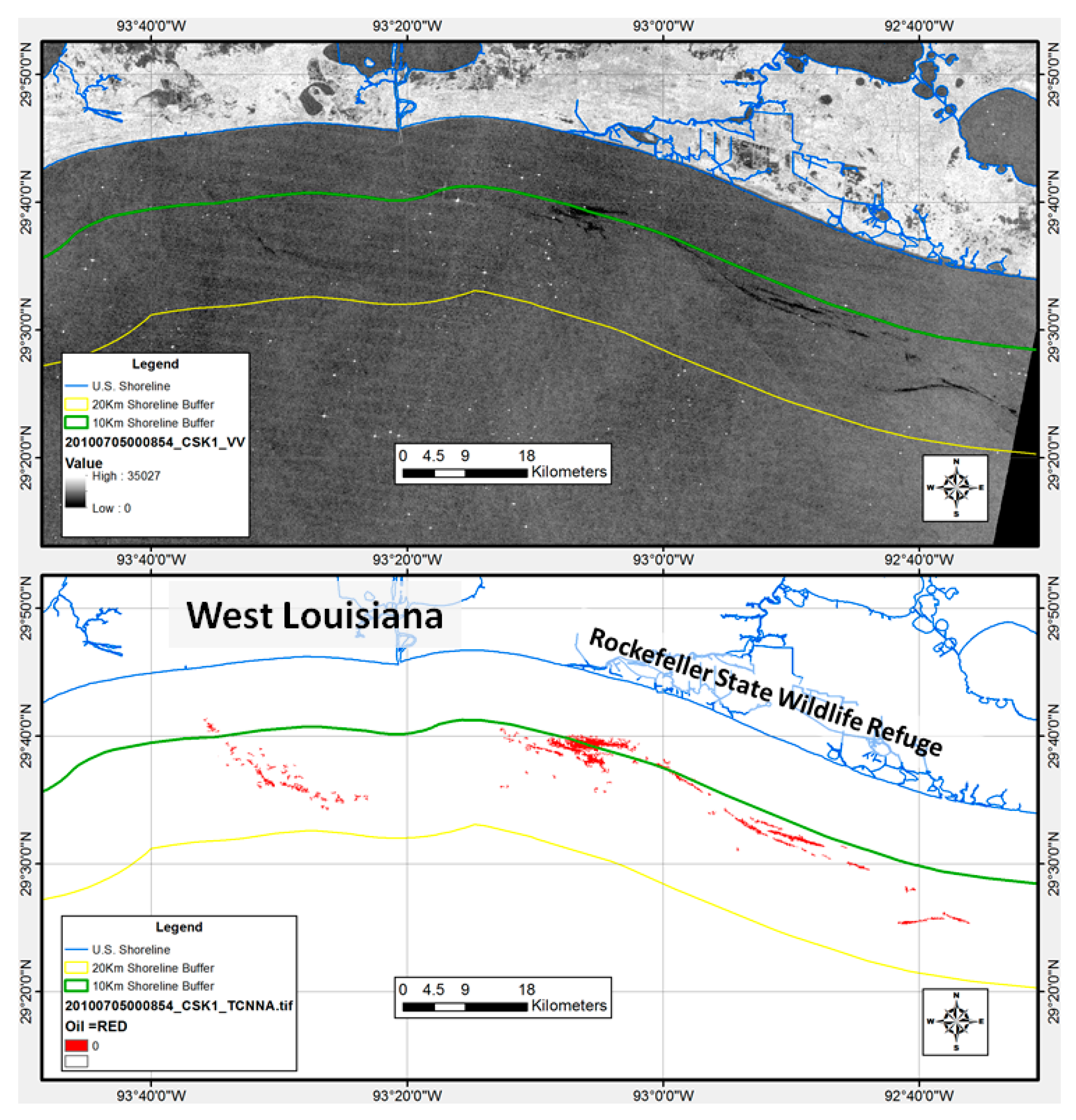
After the initial inspection of the TCNNA output, we conducted a detailed review for false positives by projecting the TCNNA output against a high resolution shoreline polygon in order to reveal those generated by land mass (Figure 5C). During this identification process, the geographic registration of the TCNNA output layer was carefully inspected and adjusted when necessary. The overlaying of the high resolution land and bathymetry layer allowed for the identification and removal of areas with low backscatter caused by land obstruction.

2.4. Shoreline Intersection

In addition to identifying oil on water in nearshore areas, we also estimated the number of days that oil was detectable within 1 km of the shoreline in selected areas. Daily composite SAR raster images were overlaid and summed using cell statistics in ArcMap (Spatial Analyst extension) to determine the number of days that oil was detected floating in proximity to the shoreline. This analysis was made on a pixel basis in open water. Because of the spatial and temporal uncertainty between the SAR data and existing shoreline in this dynamic environment, we used a buffer that allowed the shoreline and summed product to be overlaid as needed to estimate the number of days of oil exposure near the shoreline. This buffering technique generated a new raster that represented the maximum number of oiling days within a 1-km buffer from any pixel using a focal maximum algorithm to assign the maximum value from the summed raster within the search radius to the target pixel.

2.5. Statistical Analysis

We compared the maximum observed shoreline oiling to the cumulative number of days of observed oil in the water near the shoreline. This required mapping pixels in nearshore waters to a corresponding shoreline segment where oiling conditions were recorded. Shoreline segments are linear features that are tens of meters long. To assess the relationship of pixel-based oil in nearshore water, we converted the shoreline segment data into a raster layer with the same resolution as the proximate nearshore SAR data. We then overlaid the two raster data sets for comparison. We then used the Spearman’s rho rank correlation method to compare the number of SAR oiling days per pixel to the ranked order of maximum oiling (on a scale of no oiling to heavy oiling; see discussion).

3. Results

A total of 188 SAR images showing floating oil were processed using TCNNA. A subset of 156 images contained oil slicks within 10 km of the shoreline. These were the images with compliant weather conditions from 29 April to 11 August 2010, from far western Louisiana (Figure 6) to the Florida panhandle (Figure 7). They included some images that clearly show oil entering marshlands, particularly in Louisiana (see Figure 1, Figure 2 and Figure 3). The 156 images used on these results was the subset of images that comply with the ideal wind conditions for SAR to detect oil. Despite the higher potential for dampening of wind in these nearshore habitats, all of the 156 SAR images analyzed contained sufficient contrast at the edge of the slick to be clearly distinguished as oil. Only images with high gradient contrast between oil slick and surrounding areas were used for the following analysis. The surface roughness contrast allows for clear detection and delineation of surface oil. In the following section, we discuss additional ancillary data verifying that the radar anomalies in the marshes corresponded to surface oil.

Both the highest resolution SAR imagery from TerraSAR-X and medium resolution imagery from RADARSAT-1 were able to adequately detect surface oil (Figure 8, showing the red insets from Figure 1B,D). The two satellite images were taken within 12 min of each other. For most applications of oil quantification in nearshore satellite imagery, the medium resolution is sufficient for detecting oil. The areas of oil in the two images (Figure 8A,B) are detectable in the same locations on both images. Oil is apparent in both images, suggesting that wind/wave action creates surface roughness in this flat marsh habitat even in sheltered areas. While it is obvious that the higher resolution TerraSAR-X image provides more detail, the medium resolution RADARSAT-1 image from 2010 (equivalent to the current RADARSAT-2 ScanSAR resolution) captures the vast majority of the oil.

3.1. Comparison with Aerial Imagery

To validate our observations from SAR, we used supplementary oil observation data, including ground-based oil observations as well as aerial imagery that spill responders collected. Ocean Imaging Corp. (OI) collected aerial imagery of oil along the Louisiana coast on multiple days in June 2010 (Figure 9, with TCNNA-based oil coverage outlined in red). The aerial photographs taken on 8 June 2010 at 21:45 UTC were part of an OI flight mission requested by Incident Command to aid ground-based teams. The high resolution digital photographs were taken as supplemental data to other OI observations acquired in this region, from which OI generated oil classification maps on a near-daily basis throughout the three-month event [26].

Although the OI photograph and the SAR image were taken 2 h apart, the photographic evidence confirms that SAR detected floating oil in a sheltered marsh area (Figure 9), using a moderate resolution sensor (RADARSAT-1). While photographs (visible wavelengths) generally do not detect very thin sheen, SAR imagery does; hence, the greater oil extent in the SAR image (Figure 9). However, TCNNA only assesses presence or absence of oil of any thickness; it cannot discern the thick strands of oil that are evident in the photograph.

3.2. Comparison with Ground-Based Observations

As mentioned previously, during the DWH spill response, ground-based crews used SCAT to assess oil exposure on shorelines [2,16,27]. The SCAT method is a well-established and internationally recognized component of oil spill response, in use since the 1989 Exxon Valdez spill where a standard methodology for documentation, terminology, and decision-making for shoreline assessment and treatment was first applied [17]. SCAT responders survey oil stranded on shorelines (e.g., Figure 10) to determine the appropriate response actions. A SCAT survey team walks the shoreline or transits close to shore in a boat to document oiling conditions using standard terms for oil character, thickness, percent distribution, width and length of the oiled band(s), tidal zone where the oil band(s) were observed, the average and maximum size of oil deposits, and recommended cleanup tactics [2].

During the DWH spill, the SCAT teams integrated these oil observation data to classify shorelines as heavy oil, moderate oil, light oil, very light oil, or no oil observed (NOO). In areas that were repeatedly oiled such as Barataria Bay, Louisiana, the SCAT teams collected oil observation data on numerous occasions. The SCAT data do not necessarily provide data on when oil came ashore (SCAT teams could not cover all shoreline segments on all days), but the maximum oil category for each shoreline segment provides evidence of the overall degree of shoreline oiling. By contrast, daily SAR imagery can provide data on the timing of shoreline oiling, but TCNNA does not provide any information on the degree of oiling (e.g., light, moderate, or heavy).

To evaluate the relationship of these two independent oiling observation data sets in Barataria Bay, we compared the total number of days that oil was detected within 1 km of the shoreline in SAR imagery (Figure 11A) and the maximum observed shoreline oiling from SCAT data (Figure 11B). The number of observed days of oiling was positively correlated with the maximum SCAT category (p < 0.001; Figure 12), where the SCAT categories were nominally ranked from no oiling to heavy oiling. The statistical results are consistent with a visual inspection of Figure 11, which generally shows agreement between areas with high cumulative oiling days in SAR and areas with a higher degree of maximum observed oiling in SCAT. The data confirm that the likelihood of a shoreline segment being heavily oiled increases with the number of days that oil was detectable near shore in SAR imagery.

4. Discussion

During an oil spill, the planning of tactical response and damage assessment operations requires the right tools and information handy to the emergency responders [28]. For many years, satellite SAR was considered to be a tool for detecting oil in open ocean environments; oil in nearshore marsh habitats was evaluated mainly from the ground or low-flying aircraft. Cases of near-shore and onshore oil detection have been provided during the early satellite SAR days (e.g., the Empress oil spill (UK), and also from the Prestige oil spill), however limited SAR observations on those previous cases have not allowed analysis of degree of oiling in the coastal environment.

Nowadays, one of the primary advantages of satellite SAR is the number of satellites that carry SAR sensors. When a major spill such as DWH occurs, most SAR satellite operators will collect data at the spill site. This typically provides spill responders with at least one and often multiple images per day. During DWH, oil spill response used these SAR images in the open ocean to help estimate oil slick trajectories. Similar methods can be used in nearshore environments.

5. Conclusions

This paper demonstrates that satellite SAR could detect oil in Louisiana nearshore marshes on the vast majority of days during the DWH spill. SAR imagery is an additional and far less labor-intensive tool that responders can use to evaluate oiling in nearshore habitats. In addition, the workflow and process shown in this paper represents a step towards closing the time gap between the data acquisition and making available the information to the interested parties.

Once oil slicks are close to shallow waters, wind-driven surface currents and wave-induced Stokes drift [29,30] will influence the transport of the drifting oil. By collecting and analyzing a time series of SAR images in the same location, the speed and trajectory of the drifting oil in coastal areas can be estimated. In fact, outputs from algorithms such TCNNA are currently used as initialization and validation inputs for oil trajectory models [31,32]. Many oil spill models, in their simplest implementations, simulate the movement of oil on the ocean surface by tracking the movement of a large number of particles that travel at a velocity which is some combination of the ocean surface velocity and possibly surface wind. The outputs produced by this project can be used to develop, test, and validate the oil spill trajectory models on a fine scale for Gulf of Mexico coastal circulation regions.

Finally, in addition to static detection of surface oil presence and dynamic estimates of oil slick speed and trajectory, nearshore SAR imagery can provide an initial estimate of nearshore oiling impacts for multi-day (or multi-month) spills such as DWH. In this paper we describe a method for estimating nearshore oiling based on the detection of surface oil within 1 km of shore in daily satellite-based SAR composite images. Even though TCNNA cannot distinguish between a light sheen and heavy mousse, the data from Barataria Bay show that shoreline segments where oil was repeatedly detectable within 1 km were more likely to have been classified as heavily oiled by ground-based response teams conducting SCAT. This method of estimating nearshore oiling impacts from a time series of SAR images is readily available, less labor- and cost-intensive than deploying SCAT teams and aircraft, and unlike human observers, is capable of evaluating every shoreline segment every day.

References

1. Leifer, I.; Lehr, W.; Simecek-Beatty, D.; Bradley, E.; Clark, R.; Dennison, P.; Hu, Yongxiang.; Matheson, S.; Jones, C.; Holt, B.; et al. State of the art satellite and airborne marine oil spill remote sensing: Application to the BP Deepwater Horizon oil spill. Remote Sens. Environ. 2012, 124, 185–209. [Google Scholar] [CrossRef]
2. Michel, J.; Owens, E.H.; Zengel, S.; Graham, A.; Nixon, Z.; Allard, T.; Holton, W.; Reimer, D.; Lamarche, A.; White, M.; et al. Extent and Degree of Shoreline Oiling: Deepwater Horizon Oil Spill, Gulf of Mexico, USA. PLoS ONE 2013, 8, e65087. [Google Scholar] [CrossRef] [PubMed]
3. Clemente, P.; Yan, H. Low-backscatter ocean features in synthetic aperture radar imagery. Johns Hopkins APL Tech. Dig. 2000, 21, 1–6. [Google Scholar]
4. Shirvany, R.; Chabert, M.; Tourneret, Y. Ship and oil-spill detection using the degree of polarization in linear and hybrid/compact dual-pol SAR. IEEE J. Sel. Top. Appl. Earth Obs. Remote Sens. 2012, 5, 885–892. [Google Scholar] [CrossRef]
5. Holt, B. SAR Imaging of the Ocean Surface. In Synthetic Aperture Radar Marine User’s Manual; Jackson, C., Apel, J., Eds.; SAR Imaging of the Ocean Surface: Washington, DC, USA, 2004; pp. 25–80. [Google Scholar]
6. Alpers, W.; Hühnerfuss, H. Radar signatures of oil films floating on the sea surface and the Marangoni effect. J. Geophys. Res. 1988, 93, 3642–3648. [Google Scholar] [CrossRef]
7. Garcia-Pineda, O.; Zimmer, B.; Howard, M.; Pichel, W.; Li, X.; MacDonald, L.R. Using SAR Images to Delineate Ocean Oil Slicks with a Texture-Classifying Neural Network Algorith (TCNNA). Can. J. Remote Sens. 2009, 35, 411–421. [Google Scholar] [CrossRef]
8. Ramsey, E., III; Rangoonwala, A.; Suzuoki, Y.; Jones, C.E. Oil Detection in a Coastal Marsh with Polarimetric Synthetic Aperture Radar (SAR). Remote Sens. 2011, 3, 2630–2662. [Google Scholar] [CrossRef]
9. Kokaly, R.F.; Couvillion, B.R.; Holloway, J.M.; Roberts, D.A.; Ustin, S.L.; Peterson, S.H.; Khanna, S.; Piazza, S.C. Spectroscopic remote sensing of the istribution and persistence of oil from the Deepwater Horizon spill in Barataria Bay marshes. Remote Sens. Environ. 2013, 129, 210–230. [Google Scholar] [CrossRef]
10. Khanna, S.; Santos, M.J.; Ustin, S.L.; Koltunov, A.; Kokaly, R.F.; Roberts, D.A. Detection of salt marsh vegetation stress and recovery after the Deepwater Horizon oil spill in Barataria Bay, Gulf of Mexico using AVIRIS data. PLoS ONE 2013, 8, e78989. [Google Scholar] [CrossRef] [PubMed]
11. Ramsey, E., III; Rangoonwala, A.; Jones, C.E. Structural Classification of Marshes with Polarimetric SAR Highlighting the Temporal Mapping of Marshes Exposed to Oil. Remote Sens. 2015, 7, 11295–11321. [Google Scholar] [CrossRef]
12. Garcia-Pineda, O.; MacDonald, I.R.; Li, X.; Jackson, C.R.; Pichel, W.G. Oil spill mapping and measurement in the Gulf of Mexico with textural classifier neural network algorithm (TCNNA). IEEE J. Sel. Top. Appl. Earth Obs. Remote Sens. 2013, 6, 2517–2525. [Google Scholar] [CrossRef]
13. Garcia-Pineda, O.; MacDonald, I.; Hu, C.; Svejkovsky, J.; Hess, M.; Dukhovskoy, D.; Moorey, S. Detection of floating oil anomalies from the Deepwater Horizon oil spill with synthetic aperture radar. Oceanography 2013, 26, 124–137. [Google Scholar] [CrossRef]
14. Espedal, H.; Wahl, T. Satellite SAR oil spill detection using wind history information. Int. J. Remote Sens. 1999, 20, 49–65. [Google Scholar] [CrossRef]
15. MacDonald, I.R.; Guinasso, N.L., Jr.; Ackleson, S.G.; Amos, J.F.; Duckworth, R.; Sassen, R.; Brooks, J.M. Natural oil slicks in the Gulf of Mexico visible from space. J. Geophys. Res. 1993, 98, 16351–16364. [Google Scholar] [CrossRef]
16. Nixon, Z.; Zengel, S.; Baker, M.; Steinhoff, M.; Fricano, G.; Rouhani, S.; Michel, J. Shoreline oiling from the Deepwater Horizon oil spill. Mar. Pollut. Bull. 2016, 107, 170–178. [Google Scholar] [CrossRef] [PubMed]
17. National Oceanic and Atmospheric Administration (NOAA). Shoreline Assessment Manual, 4th ed.; U.S. Department of Commerce, National Oceanic and Atmospheric Administration, Office of Response and Restoration, Emergency Response Division: Seattle, WA, USA, 2013. Available online: http://response.restoration.noaa.gov/sites/default/files/manual_shore_assess_aug2013.pdf (accessed on 1 June 2017).
18. Environmental Response Management Application (ERMA). ERMA Deepwater Gulf Response Web Application. 2016. Available online: http://gomex.erma.noaa.gov/ (accessed on 1 June 2017).
19. Caruso, M.J.; Migliaccio, M.; Hargrove, J.T.; Garcia-Pineda, O.; Graber, H.C. Oil spills and slicks imaged by synthetic aperture radar. Oceanography 2013, 26, 112–123. [Google Scholar] [CrossRef]
20. Gade, M.; Alpers, W.; Hühnerfuss, H.; Masuko, H.; Kobayashi, T. Imaging of biogenic and anthropogenic ocean surface films by the multifrequency/multipolarization SIR-C/X-SAR. J. Geophys. Res. 1998, 103, 18851–18866. [Google Scholar] [CrossRef]
21. Hersbach, H.; Stoffelen, A.; De Haan, S. An improved C-band scatterometer ocean geophysical model function: CMOD5. J. Geophys. Res. Oceans 2007, 112. [Google Scholar] [CrossRef]
22. Jones, C.E.; Minchew, B.B.; Holt, B.B.; Hensley, S.S. Studies of the Deepwater Horizon Oil Spill With the UAVSAR Radar. In Monitoring and Modeling the Deepwater Horizon Oil Spill: A Record-Breaking Enterprise; Liu, Y., Macfadyen, A., Ji, Z.-G., Weisberg, R.H., Eds.; American Geophysical Union: Washington, DC, USA, 2011. [Google Scholar]
23. Minchew, B.; Jones, C.E.; Holt, B. Polarimetric analysis of backscatter from the Deepwater Horizon oil spill using L-band synthetic aperture radar. IEEE Trans. Geosci. Remote Sens. 2012, 50, 3812–3830. [Google Scholar] [CrossRef]
24. Minchew, B. Determining the mixing of oil and sea water using polarimetric synthetic aperture radar. Geophys. Res. Lett. 2012, 39, L16607. [Google Scholar] [CrossRef]
25. Couvillion, B.R.; Barras, J.A.; Steyer, G.D.; Sleavin, W.; Fischer, M.; Beck, H.; Trahan, N.; Griffin, B.; Heckman, D. Land Area Change in Coastal Louisiana from 1932 to 2010. U.S. Geological Survey Scientific Investigations Map 3164. 2011. Available online: https://pubs.usgs.gov/sim/3164/ (accessed on 31 May 2017).
26. Svejkovsky, J.; Lehr, W.; Muskat, J.; Graettinger, G.; Mullin, J. Operational Utilization of Aerial Multispectral Remote Sensing during Oil Spill Response: Lessons Learned During the Deepwater Horizon (MC-252) Spill. Photogr. Eng. Remote Sens. 2012, 78. [Google Scholar] [CrossRef]
27. Owens, E.H.; Sergy, G.A. The SCAT Manual: A Field Guide to the Documentation and Description of Oiled Shorelines, 2nd ed.; Environment Canada: Edmonton, AB, Canada, 2000; p. 108. [Google Scholar]
28. Streett, D.D. NOAA’S Satellite Monitoring of Marine Oil. In Monitoring and Modeling the Deepwater Horizon Oil Spill: A Record-Breaking Enterprise; Liu, Y., Macfadyen, A., Ji, Z.-G., Weisberg, R.H., Eds.; American Geophysical Union: Washington, DC, USA, 2011. [Google Scholar]
29. Liu, Y.; Weisberg, R.H.; Hu, C.; Zheng, L. Tracking the Deepwater Horizon oil spill: A modeling perspective. EOS Trans. Am. Geophys. Union 2011, 92, 45–46. [Google Scholar] [CrossRef]
30. Macfadyen, A.; Watabayashi, G.Y.; Barker, C.H.; Beegle-Krause, C.J. Tactical Modeling of Surface Oil Transport during the Deepwater Horizon Spill Response. In Monitoring and Modeling the Deepwater Horizon Oil Spill: A Record-Breaking Enterprise; Liu, Y., Macfadyen, A., Ji, Z.-G., Weisberg, R.H., Eds.; American Geophysical Union: Washington, DC, USA, 2011. [Google Scholar]
31. Cheng, Y.; Li, X.; Garcia-Pineda, O.; Xu, Q.; Baltazar, O.; Pichel, B. SAR observation and model tracking of an oil spill event in coastal waters. Mar. Pollut. Bull. 2011, 62, 350–363. [Google Scholar] [CrossRef] [PubMed]
32. Liu, Y.; MacFadyen, A.; Ji, Z.-G.; Weisberg, R.H. Monitoring and Modeling the Deepwater Horizon Oil Spill: A Record-Breaking Enterprise; Geophysical Monograph Series; American Geophysical Union: Washington, DC, USA, 2011; Volume 195. [Google Scholar]
Figure 1. Examples of SAR images collected over the Barataria Bay area. (A) RADARSAT-2 collected on 24 May 2010 at 12:04 UTC; (B) RADARSAT-1 collected on 8 June 2010 at 23:45 UTC; (C) Envisat collected on 9 June 2010 at 03:56 UTC; (D) TerraSAR-X collected on 8 June 2010 at 23:57 UTC; (E) ALOS-1 collected on 26 June 2010 at 16:25 UTC; and (F) COSMO-SkyMed collected on 4 June 2010 at 23:56 UTC. The blue and yellow lines are the same in all images and denote an area of particular interest during the DWH spill, extending approximately from the Mississippi River westward to Terrebonne Bay along the central Louisiana coast. The areas within the red boxes are discussed in the text.
Remotesensing 09 00567 g001
Figure 2. Sequence of SAR observations by UAVSAR (aerial SAR sensor) on 23 June 2010 (A,B); and RADARSAT-2 on 25 June 2010 (C). Both UAVSAR and RADARSAT were able to detect the oil in the nearshore environment. (Figure 2B reproduced from Jones et al. [17], used by permission).
Remotesensing 09 00567 g002
Figure 3. Examples of wind conditions observed on the SAR dataset: (A) an example of oil slicks detected by RADARSAT-2 on 21 July 2010 at 23:52 UTC during high winds; and (B) an example of oil slicks becoming undetectable in low wind conditions as imaged by RADARSAT-2 on 1 June 2010 at 12:01 UTC.
Remotesensing 09 00567 g003
Figure 4. SAR image collected by ENVISAT on 19 June 2010 at 16:01 UTC. Stormy weather complicates the identification of oil on SAR imagery. This image shows a typical summer storm pattern in the Gulf, with bright regions showing rain cells and dark regions of low backscatter corresponding to low wind cells. Images collected during conditions like this were discarded from the analysis.
Remotesensing 09 00567 g004
Figure 5. Steps taken to analyze a SAR image collected by RADARSAT-1 on 8 June 2010 at 23:45 UTC: (A) Processed 16-bit SAR data showing some dark features corresponding to low wind or land obstruction. (B) Processed TCNNA output on top of the SAR image, where backscatter anomalies that TCNNA identified as oil are shown in red. Overlaying the binary TCNNA output on top of the SAR image helps the analyst identify false positives. (C) Processed TCNNA output overlaid on a high resolution shoreline to mask the land and ensure the exclusion of false positives from proximity to land.
Remotesensing 09 00567 g005
Figure 6. (Top) SAR image collected by CosmoSky-Med 1 on 5 July 2010 (00:08 UTC) showing oil slicks in western Louisiana; and (Bottom) TCNNA output (detectable oil) is shown in red.
Remotesensing 09 00567 g006
Figure 7. (Top) SAR image collected by RADARSAT-2 on 29 June 2010 (11:43 UTC) showing oil slicks near the Florida panhandle: and (Bottom) TCNNA output (detectable oil) is shown in red. The radar-dark pixels are oil; the bright pixels are rain showers.
Remotesensing 09 00567 g007
Figure 8. Comparison of very high and medium SAR resolution: (A) TerraSAR-X collected on 8 June 2010 at 23:57 UTC with 2.3 m resolution; and (B) RADARSAT-1 collected on 8 June 2010 at 23:45 UTC with 24 m resolution.
Remotesensing 09 00567 g008
Figure 9. Comparison of apparent surface oil in an aerial photograph (top) and a quasi-contemporaneous SAR image (bottom, black outline). The TCNNA output (outlined in red) is projected over the original SAR satellite image used as background. This process is useful to ensure the alignment and geo-rectification of the oil output matches the land features. OI took the aerial image approximately two hours before the SAR image.
Remotesensing 09 00567 g009
Figure 10. Stranded shoreline oil in Terrebonne Bay, Louisiana, on 25 May 2010. SAR imagery detected this oil before and after landfall (e.g., Figure 1). This photograph was taken by the SCAT teams and archived by NOAA. This methodology for collection of this photography includes a geo-tag on the photograph along with the date and time when the snapshot was taken.
Remotesensing 09 00567 g010
Figure 11. (A) Number of days that SAR detected oil within 1 km of the shoreline; and (B) the maximum oiling that SCAT teams found after multiple ground surveys in Barataria Bay, LA.
Remotesensing 09 00567 g011
Figure 12. Correlation of cumulative number of days that oil was detectable within 1 km of the shoreline (“Cumulative SAR Days”) and maximum SCAT category (ranked from no observed oil (NOO) to heavy oil). The “tarball” category (Figure 11B) was excluded because tarballs are ranked separately in SCAT; however, this removed less than 1.5% of the categorized shoreline in Figure 11B.
Remotesensing 09 00567 g012