
A New Radiometric Correction Method for Side-Scan Sonar Images in Consideration of Seabed Sediment Variation


1
Institute of Marine Science and Technology, Wuhan University, Wuhan 430079, China
2
School of Geodesy and Geomatics, Wuhan University, Wuhan 430079, China
3
School of Power and Mechanical Engineering, Wuhan University, Wuhan 430072, China
*
Author to whom correspondence should be addressed.
Remote Sens. 2017, 9(6), 575; https://doi.org/10.3390/rs9060575
Submission received: 12 April 2017
/
Revised: 28 May 2017
/
Accepted: 6 June 2017
/
Published: 8 June 2017
(This article belongs to the Section Ocean Remote Sensing)
Abstract
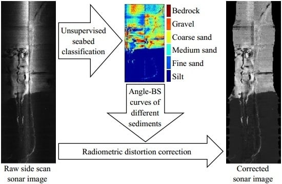
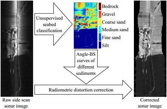
:Affected by the residual of time varying gain, beam patterns, angular responses, and sonar altitude variations, radiometric distortion degrades the quality of side-scan sonar images and seriously affects the application of these images. However, existing methods cannot correct distortion effectively, especially in the presence of seabed sediment variation. This study proposes a new radiometric correction method for side-scan sonar images that considers seabed sediment variation. First, the different effects on backscatter strength (BS) are analyzed, and along-track distortion is removed by establishing a linear relationship between distortion and sonar altitude. Second, because the angle-related effects on BSs with the same incident angle are the same, a novel method of unsupervised sediment classification is proposed for side-scan sonar images. Finally, the angle–BS curves of different sediments are obtained, and angle-related radiometric distortion is corrected. Experiments prove the validity of the proposed method.
1. Introduction
A side-scan sonar (SSS) can efficiently investigate large-area seabeds [1], and the images it captures are often used to reflect seabed geomorphology and sediment characteristics [2]; therefore, SSS is widely used in sediment classification [3,4,5], target recognition [6], and so on. SSS has long been used for seabed imaging in relatively deep water areas (e.g., large lakes and oceans), but it is currently undergoing a resurgence as systems become increasingly cheap, portable, and useful in shallow water environments, such as rivers [7,8] and coastal areas.
SSS images are formed by transferring the backscatter strength (BS) to the gray level. In SSS measurement, along-track BS is influenced by transmission loss and sonar altitude [9], whereas across-track BS is affected by transmission losses, beam patterns, angular responses of different sediments, and incident angle variations induced by seabed topography [10]. These effects cause significant radiometric distortion in SSS images, degrade image quality, and limit the application of such images [10]. Many scholars have studied methods of eliminating these effects [9,10,11,12,13,14,15]. Time varying gain (TVG) is often used to compensate for transmission losses through the use of a theoretical formula [11]. However, TVG cannot always accurately compensate for transmission losses in applications due to the use of improper or empirical parameters, so radiometric distortion induced by TVG residuals appears in SSS images. The approaches of correcting beam patterns range from simple models of Lambertian scattering [16] to complex models of sonar sensitivity that are contingent on sonar aperture, frequency, and transducer dimensions [7,17]. The effects of beam pattern and angular response can also be regarded as angular and can be compensated for by identifying proper angle–BS curves [9,10,14,15]. Wang [14] used the statistical distribution features of local BSs in temporal and spatial dimensions to obtain curves for radiometric correction; however, determining the local window size requires manual adjustment referring to SSS images. Capus et al. [9] eliminated the effect of sonar altitude variations, separated the effects of beam patterns and TVG residuals, and corrected SSS images. Hughes Clarke [15] used predicted beam patterns and roll compensation to correct the radiometric distortion of SSS images. Capus et al. [10] used SSS waterfall maps to estimate correction parameters and subsequently obtained angle–BS correction curves. These studies partly considered the effects that cause radiometric distortion and improved the quality of SSS images to some degree, but they ignored the effect of seabed sediment. Sediment effects on angle–BS curves are significant and should be considered, especially when sediment variations exist [12]. For water areas, seabed sediment types and distributions can be obtained from prior information, such as pre-investigations or sediment samples from the field. However, prior knowledge is usually unavailable. Therefore, unsupervised sediment classification on SSS images is often adopted in studies [13]. Meanwhile, sediment types cannot be accurately determined in SSS images polluted by radiometric distortion.
To solve these problems, the present study proposes a new radiometric correction method for SSS images that considers sediment variations. The paper is divided into seven sections. In Section 2, the effects that cause radiometric distortion and their characteristics are analyzed. In Section 3, the proposed method is explained in detail, along with the removal of along-track effects, a novel unsupervised sediment classification method, and angle-related radiometric correction. In Section 5, experiments are performed to assess and verify the proposed method.
2. Radiometric Distortion
Conventional SSSs use projectors on port and starboard sides to emit a wide (usually 40–60°) single beam pointing at a special graze angle (e.g., 20°) [5]. Then, the hydrophones on the port and starboard sides receive and record backscatter echoes from only one side at a fixed time interval (i.e., sample rate).
Radiometric distortion in SSS images is caused mainly by transmission losses, beam patterns, angular responses of different sediments, and incident angle variations due to topography changes. The influencing mechanisms of these factors are introduced as follows.
2.1. TVG Residuals
Acoustic waves experience spreading and absorption losses when traveling through sea water [18]. TVG is often applied to compensate for these losses.
where TL is the transmission loss, R is the spreading range expressed as propagation time t multiplied by sound velocity v, and α is the attenuation coefficient.
Given that exact α and v cannot always be obtained in the field, their empirical values are used in the compensation, which results in TVG residuals in the along-track and across-track BSs and corresponding SSS images. Moreover, TVG is difficult to redo because actual BSs are transformed by manufacturers into values with a special range and recorded in SSS XTF files. Most sonar processing packages currently use backscatter measurements scaled between 0 and 255 (8-bit quantization) or between 0 and 32,767 (16-bit quantization) [5]. In this work, the measured BSs were scaled between 0 and 32,767 (16 bit).
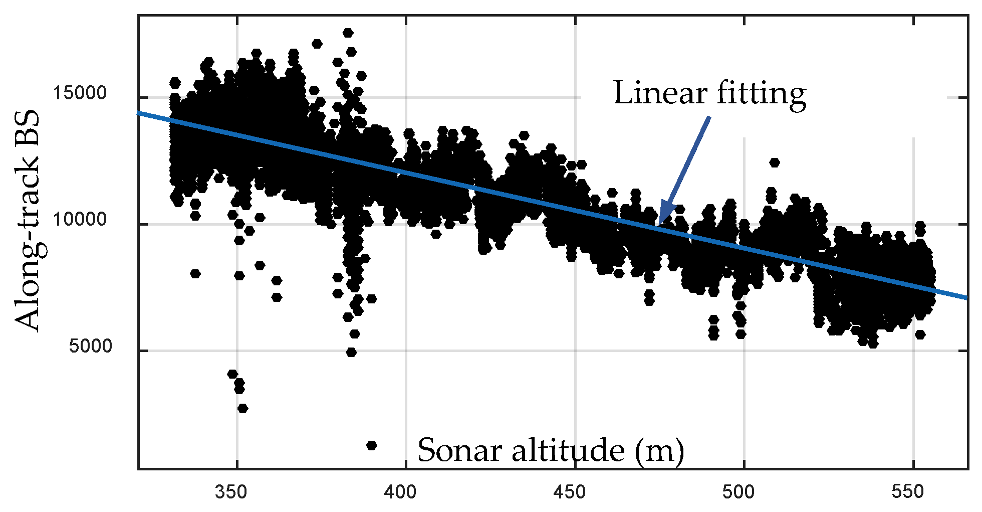
Along-track changes are complicated by BS variations introduced by changing sonar altitudes [9]; this scenario indicates that a relationship may be established between along-track TVG residuals and sonar altitudes. Figure 1 shows that BSs under the same incident angle and sediment are different and change with sonar altitudes. Moreover, an approximate linear relationship can be found between BSs and sonar altitudes. Figure 1 shows a means to remove along-track TVG residuals by using a linear function. After removing along-track TVG residuals, across-track TVG residuals remain in BSs and vary with the incident angle.
2.2. Beam Patterns
The main port and starboard lobes of an SSS are emitted according to a fixed grazing angle; thus, echoes from the seabed beneath the SSS are mainly affected by the side lobes, as shown in Figure 2a. In a ping, the BS curve of the beam pattern (Figure 2b) can be calculated [18]. The beam patterns of conventional SSSs are described in the literature [19,20]. However, beam patterns are not always perfect in practical applications, and they lead to across-track radiometric distortion in SSS images.
2.3. Angular Response
According to beam scatter patterns, the BSs of a ping vary with the incident angles of the beams. This variation is called angular response (AR). The AR effect also varies in specular and scattering domains [12]. Given that seabed impedance and roughness determine the average value and variation rate of BS, respectively, the AR effect also varies with sediment type (Figure 3a). The AR effect is usually difficult to remove due to the lack of sediment information. Combining Figure 2b with Figure 3a yields the actual angle–BS curves, which are shown in Figure 3b. The BSs received in the side-lobe area are much lower than those received in the main-lobe area; thus, the former is mainly affected by beam patterns, whereas the latter is mainly affected by the AR effect. The angle–BS curves in Figure 3b also highlight the need to consider sediment variations in radiometric correction.
3. Radiometric Correction
According to the above analyses, we divided the factors of radiometric distortion into angular unrelated and angular related. We first removed the angular-unrelated along-track TVG residual error by multiplying each ping by a reference factor. Second, we compensated for the remaining combined angular-related effects with the average angle–BS curves of individual sediments (Figure 4).
3.1. Correction of Along-Track TVG Residual
As mentioned previously, the along-track TVG residual is related to sonar altitude h. With Figure 1 as a reference, if h is obtained, then the residual effect can be removed by multiplying BS with factor fh. fh is the slope of the fitting line shown in Figure 1; it can be simply calculated as
where h0 is the given reference altitude and h is the tracked sonar altitude.
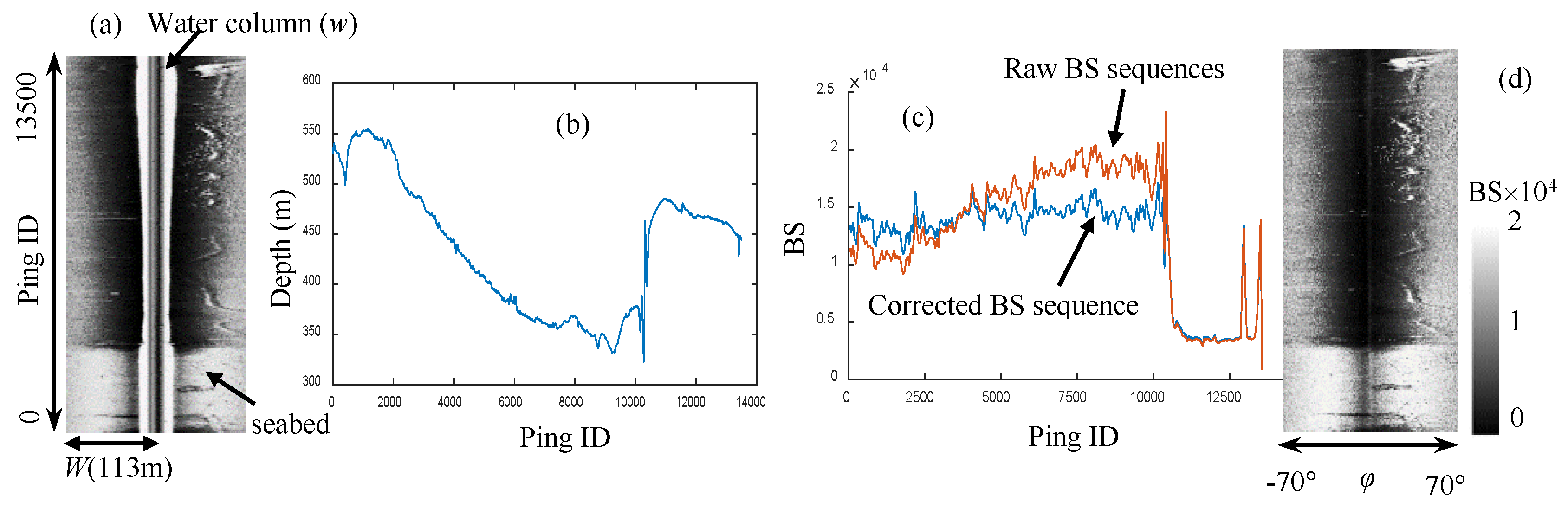
Before calculating fh, bottom tracking and geometric correction should be performed. Figure 5a shows an SSS waterfall image. The BSs in the water column are much smaller than those in the seabed area. The catastrophe point of the BS curve in a ping is also the first strong echo when the first acoustic wave reaches the seafloor. Therefore, if the inflection point is tracked, sonar altitude h can be calculated by
where Wm is the width of the waterfall image, Sm is the maximum slant range, and w is the distance from the catastrophe point to the track line or the width of the water column in Figure 5a.
A comprehensive method for bottom tracking of SSS images in complicated measuring environments [14,21] was adopted in this study to obtain accurate sonar altitude h. After bottom tracking, geometric correction of the waterfall image was conducted with
where h is the sonar altitude in the waterfall image, S is the slant distance of an echo or the distance from the echo to the track line in the waterfall image, and lh is the corresponding horizontal distance.
Taking the along-track BS sequence with an incident angle of 40° as an example, a comparison was conducted between raw and corrected along-track BS sequences, as shown in Figure 5c. The along-track BSs became almost consistent after the correction of the along-track TVG residual effect. Small changes in the sequence were produced by seabed sediment variations.
3.2. Correction of the Angle-Related Effect
According to the influential characteristics depicted in Section 2, except the along-track TVG residual effect, the effects of the across-track TVG residual, the beam pattern and angular response are related to the beam incident angle. Therefore, the SSS image distortions introduced by these effects are collectively referred to as angle-related distortion. A new angle-related distortion correction method for SSS images was also proposed. In this method, the slant-range sequence is transformed into to an angular sequence, a new unsupervised sediment classification is performed, and the angle-related distortion is corrected.
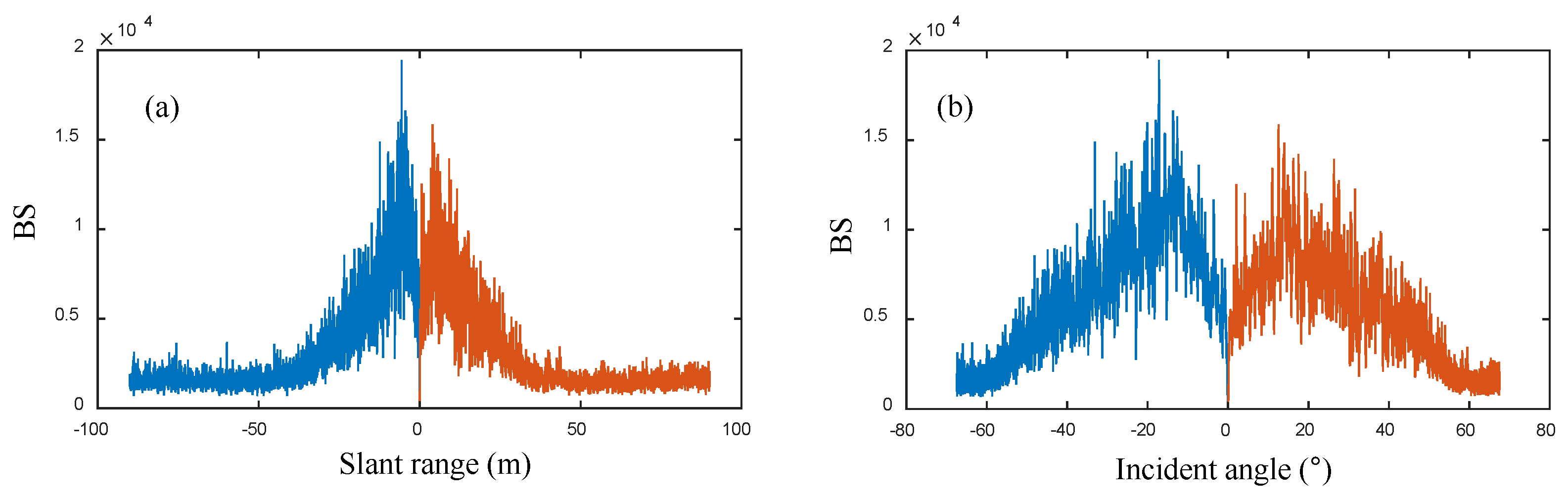
3.2.1. Slant-Range Sequence to Angular Sequence
To build the relation of the integrated effect and beam incident angles and obtain the angle–BS curves of different sediments, the slant ranges must be transformed into the incident angles of the beams (Figure 6). The transformation can be fulfilled by
where h is the sonar altitude, and S and φ are the slant range and incident angle of a beam, respectively.
When calculating the incident angles, the sonar attitude and slope of the seabed should be considered [21,22]. The yaw and pitch angles do not influence bottom tracking, whereas the roll angle influences sonar altitude in bottom tracking; this influence can be eliminated by the symmetry of the port and starboard water column widths [21]. If an inclined seabed is under the SSS sonar, the sonar altitude determined by bottom tracking will be affected, but it can be obtained accurately with the aid of the symmetry principle [21]. The undulating seabed also changes the sequence of echoes, resulting in uncertain echo locations, ambiguous areas, and incorrect horizontal distances and incident angles. Despite the use of external sounding data to calculate the incident angle in an ambiguous area based on the mechanism of SSS imaging, the correct BS, which corresponds to the angle, cannot be obtained from SSS data. Therefore, we give up the calculations of the incident angles in the ambiguous area. The ambiguous area is easily determined by the phenomenon in which a light area accompanies a shadow area in an SSS image. The above processing does not affect the succeeding steps because the final angle–BS curve of a sediment is determined by averaging all of the angle–BS curves of the sediment.
3.2.2. Unsupervised Sediment Classification
In addition to the causes of radiometric distortion, angle–BS curves significantly vary with different sediments (Figure 3). Therefore, the sediment distributions of a surveyed water area should be obtained. Sediment distributions can be determined through a pre-investigation or analysis of field samples. In the absence of prior information, sediment distributions can be obtained from SSS images with an unsupervised classification algorithm. Accurately determining sediment distributions using SSS images polluted by radiometric distortion is impossible. To solve this problem, this study developed a novel method called angle-irrelevant unsupervised sediment classification.
(1) Normalization of along-track BSs
After the removal of the along-track TVG residual effect, the angle-related effect on BSs under the same incident angle is the same. Therefore, the sediment effect on BSs can be regarded as the only effect on the along-track BSs. In such a case, the BS variations under the same incident angle can reflect sediment variations. However, BSs under different incident angles vary in terms of their ranges due to the effects of AR and beam patterns (Figure 7a). BSs with different incident angles should be normalized.
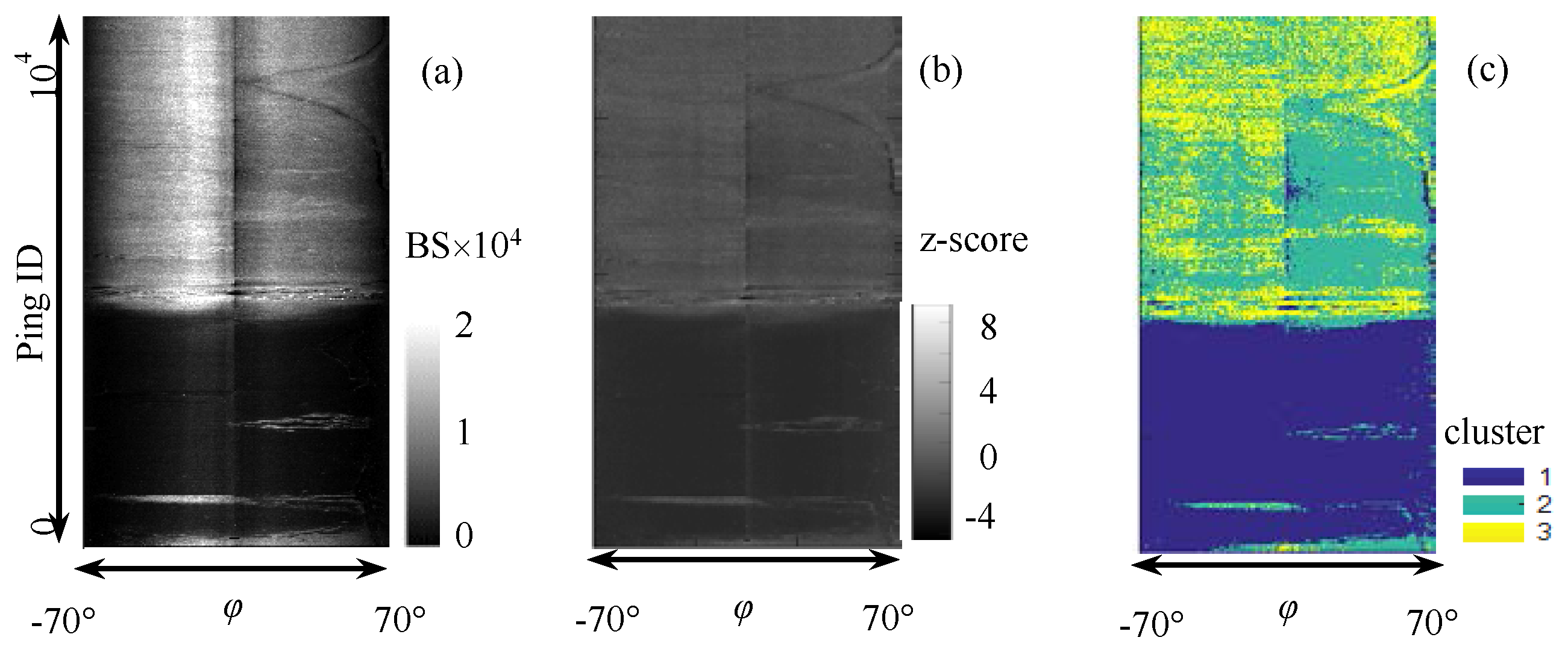
The standard score of a variable, also called the z-score, is defined as the variable minus its mean and then divided by its standard deviation; it is a common statistical technique to normalize diverse parameters to a common dynamic range [23]. For a random variable x with mean μ and standard deviation σ, the z-score of a value x is
After applying the z-score to normalize the BSs under different angles, all BSs with the same sediment types are in the same range, as shown in Figure 7b.The z-score sequences in Figure 7b show the same tendency as the BS sequences in Figure 7a and reflect sediment variation. This characteristic causes the same sediments to be classified into one.
(2) Unsupervised classification by k-means++
After normalization, the unsupervised sediment classification can be implemented by using the along-track BS sequences with different incident angles. The k-means++ algorithm provides a means of avoiding the sometimes poor results found by the standard k-means algorithm, and it offers the advantages of simplicity, speed and accuracy [24]. Therefore, the k-means++ algorithm was used in this study for unsupervised sediment classification on the normalized z-score images. The detailed procedure is shown below.
- (1)
- Transform two-dimension z-score image Iz to one-dimension vector V.
- (2)
- Use the k-means++ algorithm for the k cluster centers’ initialization of V.
- (3)
- Calculate the distance of each value in V to each centroid, and assign it to the cluster with the closest centroid.
- (4)
- Compute the average values of all the clusters to obtain k new centroid locations.
- (5)
- Repeat Steps 3 and 4 until the cluster assignments do not change and the distribution D of each value in V is obtained.
- (6)
- Transform vector D to two-dimension classification image ID.
Figure 8 depicts the procedure of the unsupervised sediment classification using an SSS image.
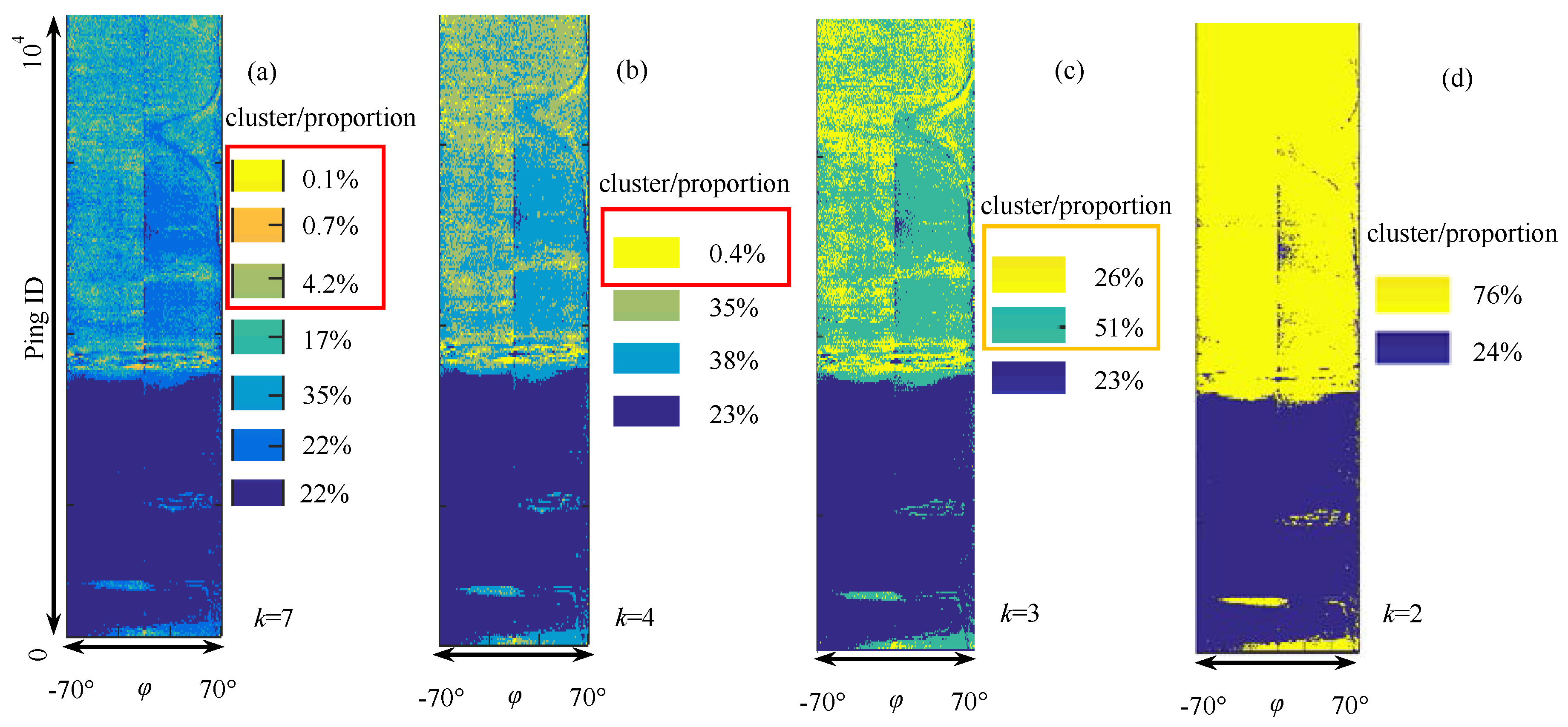
(3) Iteration method for determining classification number k
In the unsupervised classification described above, classification number k, namely, the number of sediment types, is necessary. The problem is that k cannot always be known in advance. An iteration method was therefore implemented to obtain a proper k. Given that the k-means++ cluster method assigns all BSs to several cluster centers, the value and proportion of each center represent the average BS and proportion of the corresponding sediment. When the given k is extremely large, the clusters would be numerous; to avoid this, k can be compressed into a small value. Clusters with a proportion of less than 5% should be ignored, and clusters whose distance is less than 5% of the BS variation range should be considered for merging. In this case, k is determined through the following steps.
- (1)
- Provide a large value (for example, k = 7) as the initial k.
- (2)
- Apply k-means++ on the z-score image with the initial k.
- (3)
- Calculate the center intensities and proportion of each sediment.
- (4)
- Remove the clusters whose proportion is less than 5%, and merge the clusters whose distance is less than 5% of the BS variation range. Then, a new k is obtained.
- (5)
- Repeat Steps 2–4 until k does not change.
Figure 9 depicts the procedure of determining k.
3.2.3. Radiometric Correction
After obtaining the appropriate classification number, angle-related distortion correction can be performed using the angle–BS curves of different sediments.
Based on the sediment distributions obtained through unsupervised sediment classification, the angle–BS curve (ABC) of sediment c can be obtained by statistically averaging the BSs with incident angle φ and sediment c, as shown in Equation (7).
where nc,φ is the number of BSs with incident angle φ and sediment c.
By changing φ, the angle–BS curve corresponding to the given sediment c can be obtained with Equation (7). Similarly, the angle–BS curves of all sediments can be obtained by changing c. At this point, the angle–related effects can be removed by subtracting ABC(c, φ) from the raw BS BSr(c, φ) and then adding the mean BS BS0(c), as shown in Equation (8).
where BS, BSc, and BS0 are the raw, corrected, and mean BSs, respectively.
After removing the along-track TVG residual and angle-related effects from the raw BS, the image obtained by transforming BSc to the gray level is un-affected by radiometric distortion and should exhibit high quality.
4. Process of Radiometric Distortion Correction for SSS Images
The complete procedure of radiometric correction is described below (Figure 10).
- (1)
- Use bottom line tracking to obtain the along-track sonar altitudes, calculate factor fh with Equation (2) at a given referencing sonar altitude, and remove the along-track TVG residual by multiplying BS with fh.
- (2)
- Transform the slant range to the incident angle and obtain angle–BS sequences.
- (3)
- Use the z-score to normalize the raw BSs and obtain the z-score image.
- (4)
- Apply the unsupervised cluster algorithm and obtain the distributions of different sediments.
- (5)
- Obtain the angle–BS curves of different sediments and implement radiometric correction.
- (6)
- Transform the corrected BS to the gray level and form a new SSS image.
5. Experiments and Analysis
SSS measurement was carried out in Fujian waters in 2012 to verify the proposed method. The water area measured 1.6 km × 6.0 km, and the water depth ranged from 5 m to 30 m. Four survey lines were completed with Edgetech 4100P SSS, which features 500 kHz of operating frequency, 112 m of recorded max slant range, 20° of sonar depression angle, and 0.5° and 50° of plane and vertical beam angles, respectively. Seabed surface sampling was performed with a grab sampler that measured 20 cm in thickness and covered 3600 cm2 of the seafloor at every 5″ longitude and 9″ latitude interval. Six types of sediments, namely, bedrock, gravel, coarse sand, medium sand, fine sand, and silt, were identified with a 500 μm sieve. Raw SSS BS data were recorded in *.xtf files. By decoding these SSS files, the waterfall map of each line was formed, and the geo-coding image was obtained. The geo-coding SSS image was confusing, and the sediment and target distributions in the image were difficult to recognize because the raw BS data were polluted by radiometric distortion. To apply the SSS image, radiometric distortion should be removed, and the quality of the SSS image should be improved.
5.1. Correction of Radiometric Distortion
As shown in Figure 11a, the BS data of a survey line were extracted and processed with a traditional method [14] and the proposed method to explain the data processing in the proposed method clearly. The seabed consists of two main sediments, namely, coarse sand and silt.
Figure 11a shows the raw SSS waterfall map. With the sediment variation ignored, the SSS image was corrected with the angle–BS curves obtained by statistically averaging the entire survey line (method 1) and every 50 pings in the along-track direction (method 2). The corresponding results are shown in Figure 11b,c. The result obtained by using the proposed method is shown in Figure 11d.
Influenced by radiometric distortion, the gray level was non-uniform, especially in the same sediment area; this characteristic caused that the small sediment variations and features became fuzzy shown in Figure 11a. Nevertheless, two main sediments, a transitional region of the two sediments, micro sediment variations, and small features appear in the image. The radiometric distortions shown in Figure 11a were corrected with the three methods, and the corresponding results are shown in Figure 11b–d. Figure 11d shows the best result, followed by Figure 11b,c. As shown in Figure 11b, the effect of the beam pattern remains. Moreover, the micro sediment variations in the ellipse could not be reflected accurately, and several mistaken targets appear in the rectangle area. The reason for this result was analyzed accordingly. Method 1 adopts an angle–BS curve obtained by averaging the BSs of different incident angles in the entire area. Two factors lead to an inaccurate angle–BS curve. One is the failure to consider sediment variations, and the other is using the entire polluted BS data directly. Figure 11c is better than Figure 11b, and an obvious improvement is the removal of the beam pattern effect. However, this method yields undesirable outcomes, that is, the micro sediment variations in the ellipse and the two sediment areas are smoothened away, and several features in the rectangle disappear. These phenomena are caused by the correcting mechanism of method 1. In method 2, many angle–BS curves are produced at every 50 pings by the same calculation depicted in method 1, and these curves are used to correct the corresponding 50-ping BSs. Therefore, method 2 is a refinement of method 1. The correction by method 2 seemed to remove radiometric distortion and make the image smooth. Actually, excessive filtering is observed in the correction results. Moreover, untruthfulness is further enhanced because sediment variations are ignored and polluted BS data are used. Unlike those shown in Figure 11b,c, the along-track and across-track radiometric distortions are removed, and the sediment distributions, micro sediment variations, and seabed features are clearly displayed in Figure 11d. The proposed method used in Figure 11d considers sediment variations. The sediment distributions are accurately classified because the processing steps of along-track distortion correction, normalization, and unsupervised sediment classification on the along-track BS sequences are adopted. Therefore, the effect of across-track distortion is weakened significantly, and the angle–BS curves of different sediments can be obtained accurately. Given the resolution of the problems involved in using methods 1 and 2, an ideal correction result was obtained (Figure 11d).
The histogram of the raw BSs and that of the BSs corrected with the proposed method were calculated, and the results are shown in Figure 12a,b, respectively. The distribution of the raw BSs was imbalanced, was mostly near the low value, and failed to reflect the two sediments due to radiometric distortion. After the correction, the BSs approached the center BSs of the two sediments and clearly reflected the two sediments.
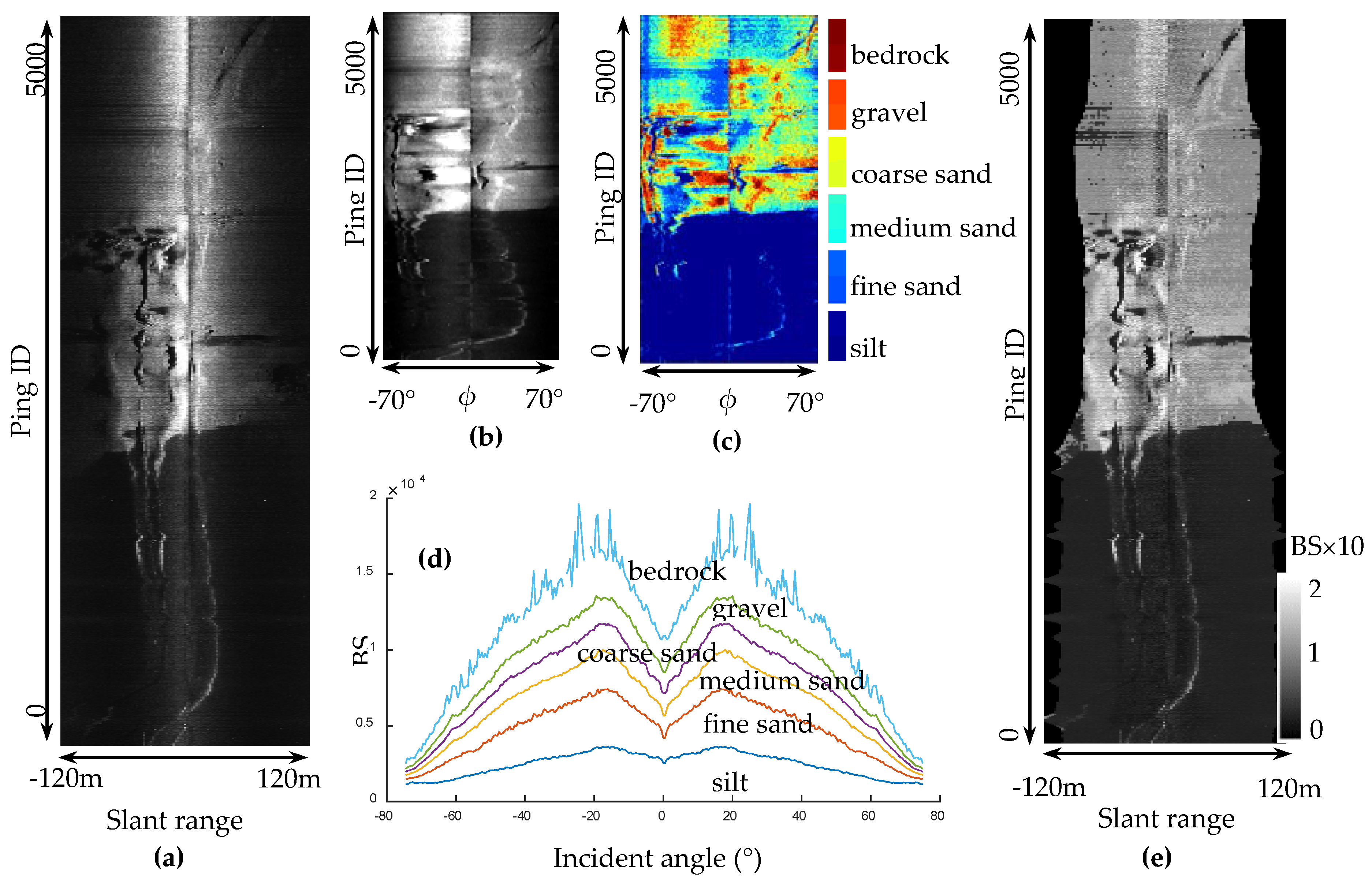
In the above experiment, the seabed consisted of only two sediments. A segment of SSS data with six types of sediments (i.e., bedrock, gravel, coarse sand, medium sand, fine sand, and silt) was extracted from the measuring data to analyze the performance of the proposed method when correcting an SSS image with various sediments (Figure 13a). The radiometric distortion in the SSS data was corrected with the proposed method. First, the SSS data were converted to an angle–BS image (Figure 13b), normalized with the z-score, and classified with the k-means++ algorithm (Figure 13c). Second, the average angle–BS curves of the six sediments were extracted (Figure 13d), and radiometric distortion was corrected (Figure 13e).
Figure 13a,b shows that the shortcomings in Figure 11a are also displayed in the images due to the effect of radiometric distortion on the SSS data. After normalization and seabed classification, the six sediments were classified, and the results are shown in Figure 13c. Figure 13d shows the curves of the six sediments. As the acoustic impedances of the six sediments (i.e., bedrock, gravel, coarse sand, medium sand, fine sand, and silt) decreased successively, the average BSs of the corresponding angle–BS curves decreased successively as well. By using the average angle–BS curves, radiometric distortion was corrected and removed from Figure 13a. In the corrected image (Figure 13e), the BSs of the same sediment were basically consistent at different incident angles. The proposed method is clearly efficient when applied to the radiometric correction of SSS images with various sediments.
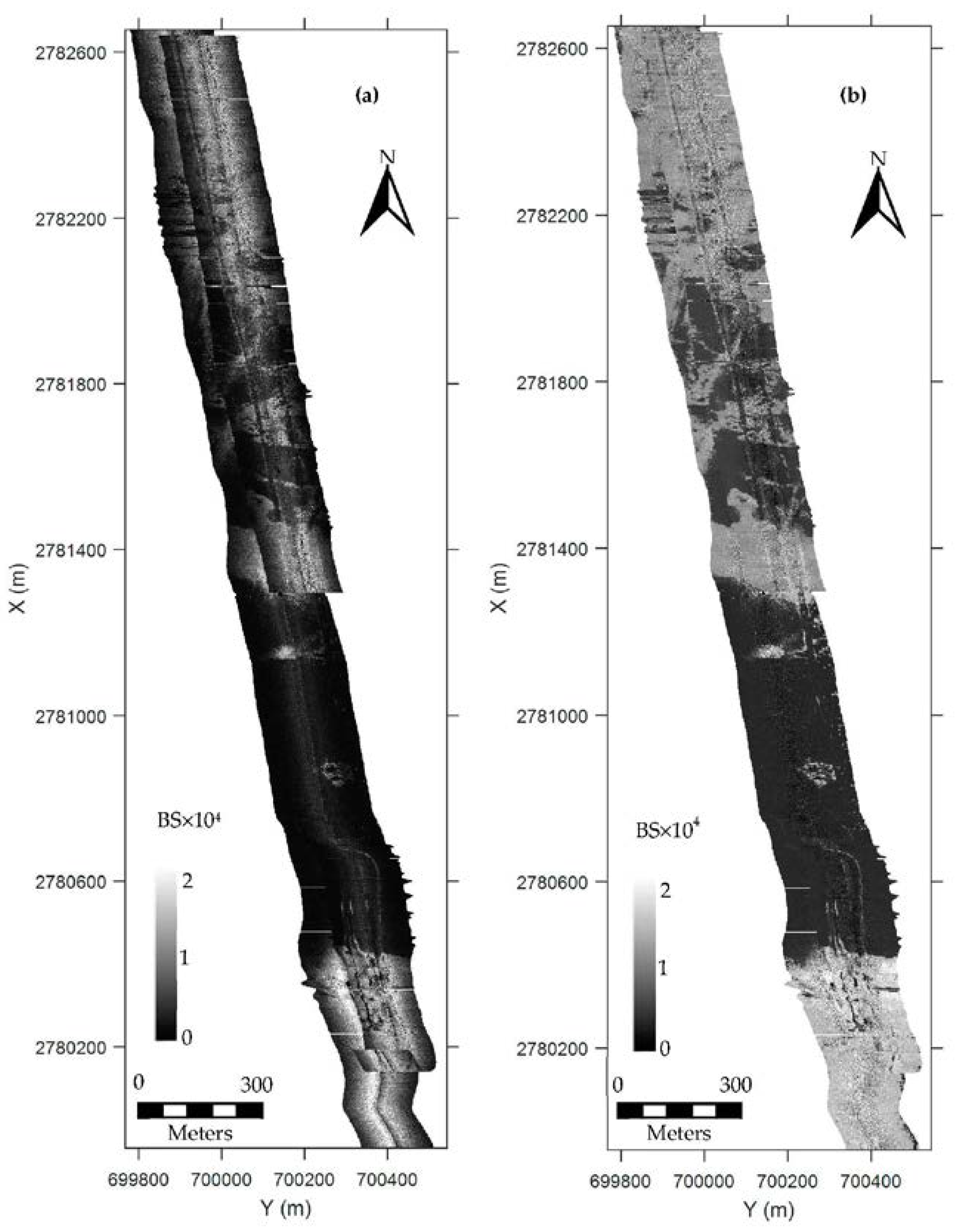
Through the same process described above, the four SSS lines measured in the surveyed water were corrected with the proposed method. Figure 14a,b show the raw and corrected images, respectively. As shown in Figure 14a, because of radiometric distortion, the raw sonar image is very disordered, and the sediment distributions, micro sediment variations, and seabed features are difficult to distinguish. For the SSS image of each line, the inner BSs are significantly higher than the outer ones. As a result, the common mosaic areas of two adjacent lines are confusing, and the topographical and sediment features in the common area are false due to the effect of the radiometric distortion. In Figure 14b, the sediment variation in the surveyed water area is clear, and the BSs of the same sediments are consistent. Even in the transition area of different sediments and the common areas of two adjacent lines, the sediment variations and distributions can also be reflected accurately. Figure 14b further proves the effectiveness of the proposed method.
5.2. Consistency Assessment
5.2.1. Co-Located Sediment Variation and Target
Given that the co-located sediment variations of two adjacent survey lines are the same, the corresponding sonar images should represent the variations. However, for raw SSS images, BSs are affected not only by sediment variations but also by radiometric distortion. As a result, the co-located sediment variations in the two lines become inconsistent. If the conflict is eliminated with the proposed method, the satisfactory performance of the proposed method will be proven.
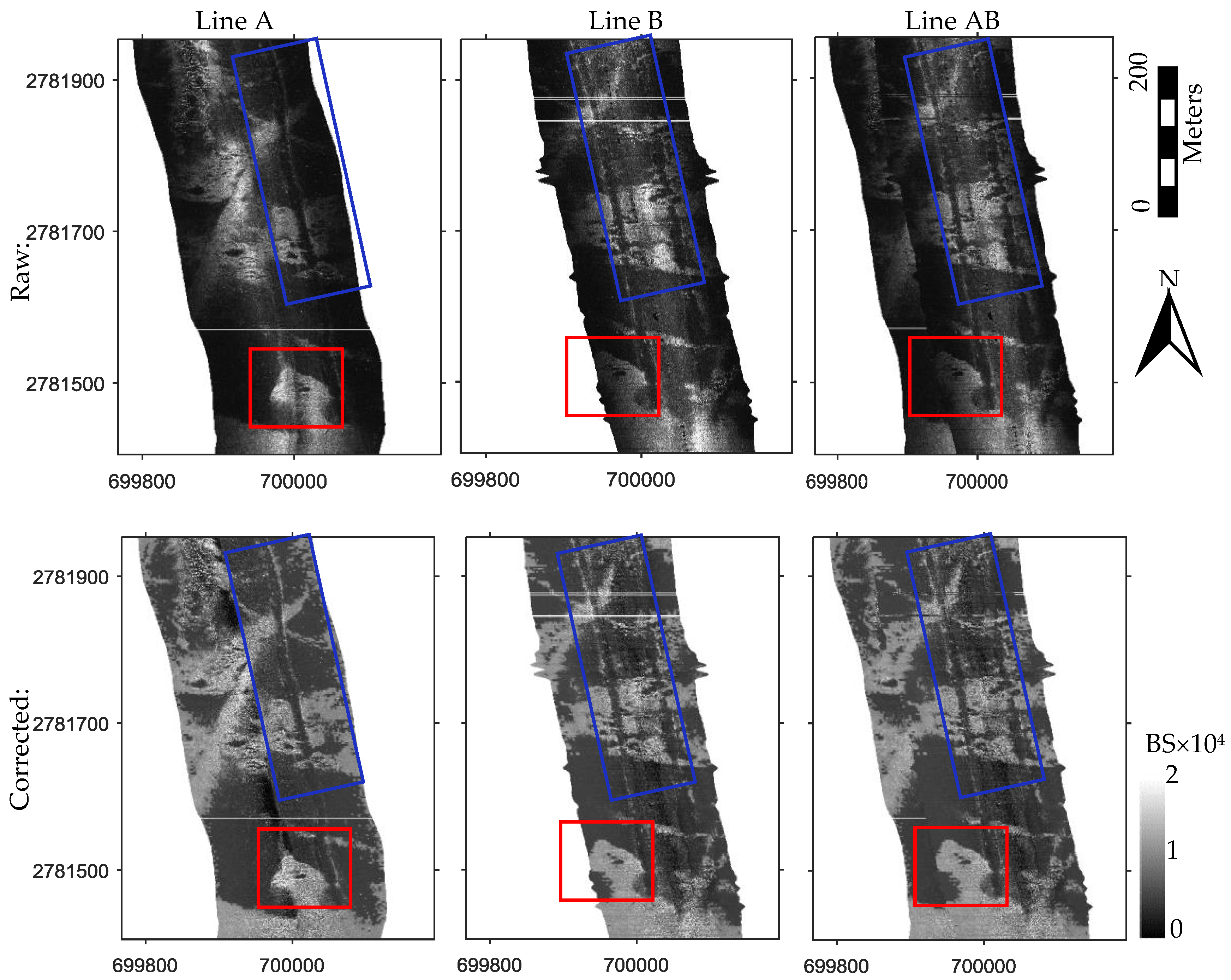
Two adjacent survey lines with rich sediment variations (i.e., Lines A and B) were selected and corrected to assess the consistency of the co-located sediment variations, as shown in Figure 15. The raw images are confusing, leading to unclear sediment distributions and inaccurate shapes of seabed targets. The situation is reversed in the corrected images. A peach-shaped sediment distribution marked with a red rectangle and two submarine pipes marked with a blue rectangle were selected to analyze the performance and function of the proposed method. The peach-like shape exists in Lines A and B. For Line A, it appears in the inner region, which is mainly affected by the beam pattern. For Line B, the shape appears in the outer region, which is mainly affected by the angular response. One of the two pipelines appears in the right-hand side of Line A and the left-hand side of Line B. The other lines appear in the right-hand side of Line B. Both lines are affected by the angular response. As a result of the radiometric effect, the peach-like shape in raw Line A is distorted, whereas that in raw Line B is not complete and even disappears in the mosaic image. The same situation was observed in the two pipelines. Conversely, the peach-like shapes, the pipelines in the corrected Lines A, B, and AB are consistent. The experiment showed that the proposed method effectively guarantees the shapes and consistency of seabed targets.
5.2.2. Co-Located BSs
As a result of radiometric distortion, the BSs in the co-located region of two survey lines differ significantly. After radiometric correction, BSs should be consistent. Depending on this fact, the co-located BS consistency of the two overlapped survey lines was used to assess the validity of the proposed method.
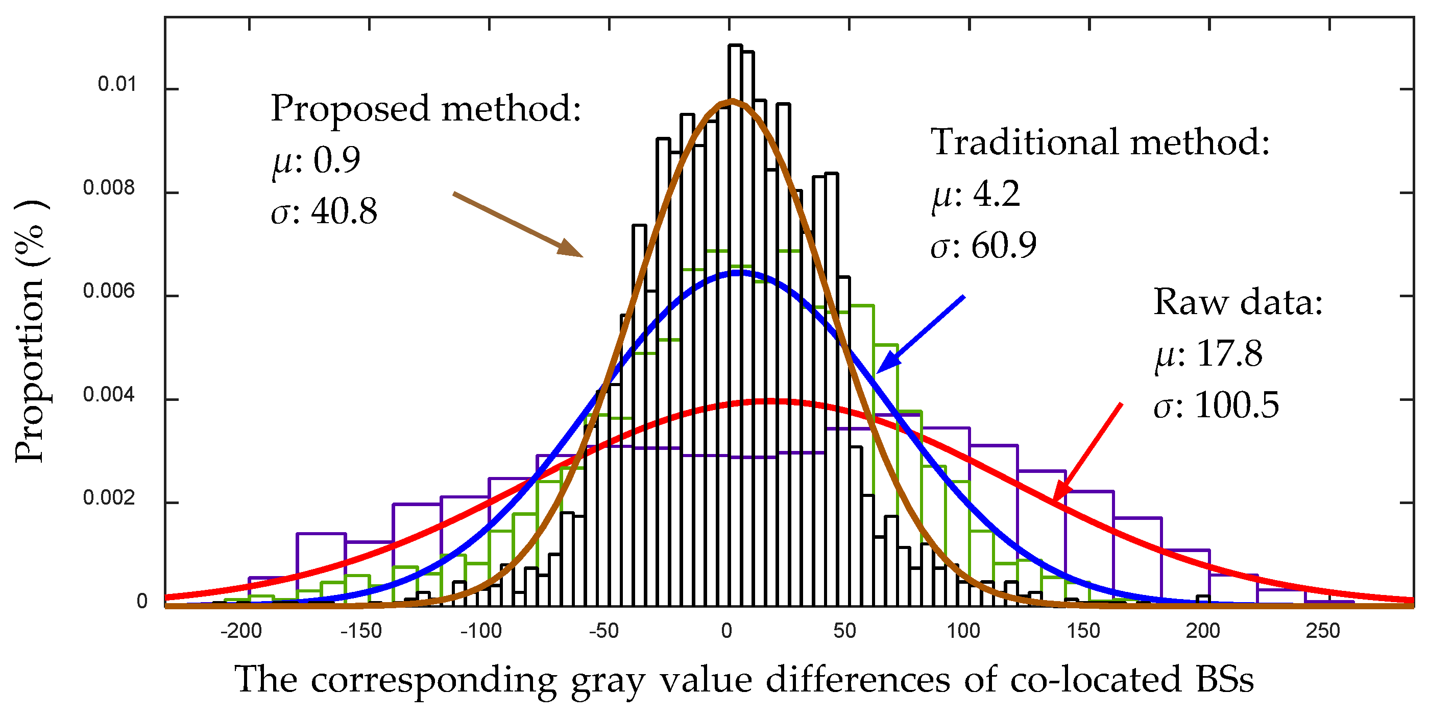
All overlapped areas of different adjacent lines were selected for the assessment. For comparison, statistical results and fitting probability density functions (PDF) of raw, and corrected data using the traditional method depicted in [9] and proposed method, respectively, were calculated, as shown in Figure 16. The raw BS data showed systematic bias and a large-range bias distribution, whereas the corrected BS data using the proposed method exhibited a smaller mean bias and standard deviation relative to the raw and corrected data using the traditional method. Furthermore, the bias of the corrected BS data using the proposed method followed a Gaussian distribution. The statistical results also showed that the proposed method efficiently removed the radiometric distortion effect, ensured the BS consistency of overlapped survey lines, and improved the quality of raw SSS images. The experiment proves the validity of the proposed method.
6. Discussion
6.1. Application of the Proposed Method
SSS has been widely used in relatively deep waters and even in shallow water environments, such as rivers [7,8] and coastal areas. Notably, SSS is no longer reserved for geological oceanographers and hydrographers but has been increasingly applied in hydrology and ecology. Therefore, the radiometric correction method proposed in this study can be applied to any side-scan imagery from any environment.
6.2. Other Sediment Classification Algorithms
The k-means++ algorithm was used for sediment classification in this study. However, the specific approach to sediment classification proposed in this study is not crucial, and others with equal effectiveness could be used. Many other side-scan sediment classification approaches are discussed in related literature, such as those proposed by Buscombe et al. [25] and Burguera and Oliver [17], in which each pixel is classified into one of several discrete classes. Several sediment classification approaches work better than others in specific environments. Owing to the fact that correction of side-scan imagery is not predicated on a particular sediment classification algorithm, an appropriate sediment classification method should be adopted according to the special condition.
6.3. Other Influential Factors
The radiometric distortion caused by sediment variation includes three terms: the average angular response per sediment (as discussed in this study), the angular response per sediment patch (angular response caused by within-sediment variability), and noise that is unrelated to sediment. By computing an average substrate-specific angular response curve and applying this curve to all regions of the image representing that substrate, the small differences in the angular response curves within individual substrates are assumed to be insignificant to radiometric distortion.
Direct correlations between side-scan backscatter magnitude and grain size, such as those adopted in the current work, have been previously established [26,27], but in other situations, image texture is more indicative of grain size, and backscatter magnitudes are not good discriminators [25,28]. The latter might be the case in the presence of a significant amount of morphological variability (such as bedforms and ranges of bed slopes) within individual sediment types (silt, sand, gravel, etc.).
6.4. Related Work in the Multibeam Sonar Aspect
Since the multibeam sonar have many similarities to SSS, the correction method for multibeam imagery could also referred in the side-scan processing. The angular dependence of 12 Hz seafloor acoustic backscatter was introduced by de Moustier and Alexandrou [29]. Fernandes and Chakraborty [30] processed the correction of the angular response and beam pattern of EM 1002 multibeam sonar. Applications of using the multibeam sonar data for seabed classification have also been introduced in many studies [31,32,33,34]. Notably, the multibeam sonar and SSS suffer from the same angular response effect, but they have different beam pattern effects. SSS imagery is more easily affected by seabed morphological variability in comparison with multibeam sonar imagery.
7. Conclusions
This study proposed a new radiometric correction method for SSS images that considers sediment variation. In the proposed method, the radiometric effects on BSs with the same incident angle become similar due to the correction of the along-track TVG residual. After normalization, the BS sequences with different incident angles vary in approximately the same range. Sediment classification using the normalized along-track BS sequences was performed with the k-means++ cluster algorithm, which ensures that the classification is not disturbed by angle-related effects. Thus, the average angle–BS curves of different sediments can be established accurately according to the sediment classification. With these new algorithms, the performance of the proposed method is guaranteed, the radiometric effect is removed effectively, and high-quality SSS images are obtained. These conclusions were proven by the experiments. In the experiments, the average and standard deviation of the gray value differences of the co-located echo strengths of different survey lines deceased from 17.8 to 0.9 and from 100.5 to 40.8, respectively.
Acknowledgments
The research is supported by the National Natural Science Foundation of China (Coded by 41376109, 41576107, and 41176068), National Science and Technology Major Project (Coded by 2016YFB0501703), and the Key Laboratory of Surveying and Mapping Technology on Island and Reef, National Administration of Surveying, Mapping and Geoinfomation (coded by 2015B08). The data in this paper are provided by the Guangzhou Marine Geological Survey Bureau. The authors are thankful for this support.
Author Contributions
Jianhu Zhao and Jun Yan conceived and designed the experiments; Jun Yan performed the experiments; Jun Yan and Junxia Meng analyzed the data; Hongmei Zhang contributed the analysis tools; and Jianhu Zhao, Jun Yan, Hongmei Zhang and Junxia Meng wrote the manuscript.
Conflicts of Interest
The authors declare no conflict of interest.
References
- Kaeser, A.J.; Litts, T.L.; Tracy, T. Using low-cost side-scan sonar for benthic mapping throughout the lower flint river, Georgia, USA. River Res. Appl. 2013, 29, 634–644. [Google Scholar] [CrossRef]
- Powers, J.; Brewer, S.K.; Long, J.M.; Campbell, T. Evaluating the use of side-scan sonar for detecting freshwater mussel beds in turbid river environments. Hydrobiologia 2015, 743, 127–137. [Google Scholar] [CrossRef]
- Haniotis, S.; Cervenka, P.; Negreira, C.; Marchal, J. Seafloor segmentation using angular backscatter responses obtained at sea with a forward-looking sonar system. Appl. Acoust. 2015, 89, 306–319. [Google Scholar] [CrossRef]
- Grządziel, A.; Felski, A.; Wąż, M. Experience with the use of a rigidly-mounted side-scan sonar in a harbour basin bottom investigation. Ocean Eng. 2015, 109, 439–443. [Google Scholar]
- Blondel, P. The Handbook of Sidescan Sonar; Springer Science & Business Media: Berlin, Germany, 2010. [Google Scholar]
- Schultz, J.J.; Healy, C.A.; Parker, K.; Lowers, B. Detecting submerged objects: The application of side scan sonar to forensic contexts. Forensic Sci. Int. 2013, 231, 306–316. [Google Scholar] [CrossRef] [PubMed]
- Buscombe, D. Shallow water benthic imaging and substrate characterization using recreational-grade sidescan-sonar. Environ. Model. Softw. 2017, 89, 1–18. [Google Scholar] [CrossRef]
- Kaeser, A.J.; Litts, T.L. A novel technique for mapping habitat in navigable streams using low-cost side scan sonar. Fisheries 2010, 35, 163–174. [Google Scholar] [CrossRef]
- Capus, C.; Ruiz, I.T.; Petillot, Y. Compensation for changing beam pattern and residual tvg effects with sonar altitude variation for sidescan mosaicing and classification. In Proceedings of the 7th European Conference Underwater Acoustics, Delft, The Netherlands, 5–8 July 2004. [Google Scholar]
- Capus, C.G.; Banks, A.C.; Coiras, E.; Ruiz, I.T.; Smith, C.J.; Petillot, Y.R. Data correction for visualisation and classification of sidescan SONAR imagery. IET Radar Sonar Navig. 2008, 2, 155–169. [Google Scholar] [CrossRef]
- Moreira, M.A.; Vital, H.; Lira, N.B.H.F. Using side scan sonar in the characterization of the continental shelf: Touros area. In Proceedings of the 2013 IEEE/OES, Acoustics in Underwater Geosciences Symposium (RIO Acoustics), Rio de Janeiro, Brazil, 24–26 July 2013; pp. 1–5. [Google Scholar]
- Zhao, J.; Yan, J.; Zhang, H.; Meng, J. Two self-adaptive methods of improving multibeam backscatter image quality by removing angular response effect. J. Mar. Sci. Technol. 2017, 22, 288–300. [Google Scholar] [CrossRef]
- Andersson, A.J.; Reed, T.B.; Winn, C.D. Marine sediment classification using sidescan sonar and geographical information system software in Kaneohe Bay, Oahu, Hawaii. In Proceedings of the Oceans, 2001 MTS/IEEE Conference and Exhibition, Honolulu, HI, USA, 5–8 November 2001; IEEE: Honolulu, HI, USA, 2001; Volume 4, pp. 2653–2657. [Google Scholar]
- Wang, A. Research on 3D Seafloor Terrian Recovery from the Side Scan Sonar Image; Wuhan University: Wuhan, China, 2014. [Google Scholar]
- Hughes Clarke, J.E. Seafloor characterization using keelmounted sidescan: Proper compensation for radiometric and geometric distortion. In Proceedings of the Canadian Hydrographic Conference, Ottawa, ON, Canada, 25–27 May 2004. [Google Scholar]
- Mitchell, N.C.; Somers, M.L. Quantitative backscatter measurements with a long-range side-scan sonar. IEEE J. Ocean. Eng. 1989, 14, 368–374. [Google Scholar] [CrossRef]
- Burguera, A.; Oliver, G. High-Resolution Underwater Mapping Using Side-Scan Sonar. PLoS ONE 2016, 11, e0146396. [Google Scholar] [CrossRef] [PubMed]
- Waite, A.D. Sonar for Practising Engineers, 3rd ed.; John Wiley & Sons Incorporated: Chichester, UK, 2002. [Google Scholar]
- Chang, Y.-C.; Hsu, S.-K.; Tsai, C.-H. Sidescan sonar image processing: Correcting brightness variation and patching gaps. J. Mar. Sci. Technol. 2010, 18, 785–789. [Google Scholar]
- Mazel, C. Side Scan Sonar Record Interpretation; Klein and Associates, Inc.: Salem, NH, USA, 1985. [Google Scholar]
- Zhao, J.; Wang, X.; Zhang, H.; Wang, A. A Comprehensive Bottom-Tracking Method for Sidescan Sonar Image Influenced by Complicated Measuring Environment. IEEE J. Ocean. Eng. 2016. [Google Scholar] [CrossRef]
- Honsho, C.; Ura, T.; Asada, A.; Kim, K.; Nagahashi, K. High-resolution acoustic mapping to understand the ore deposit in the Bayonnaise knoll caldera, Izu-Ogasawara arc. J. Geophys. Res. Solid Earth 2015, 120, 2070–2092. [Google Scholar] [CrossRef]
- Fonseca, L.; Calder, B. Clustering acoustic backscatter in the angular response space. In Proceedings of the US Hydrographic Conference, Norfolk, VA, USA, 14–18 May 2007. [Google Scholar]
- Arthur, D.; Vassilvitskii, S. K-means++: The advantages of careful seeding. In Proceedings of the Advances in the Eighteenth Annual ACM-SIAM Symposium on Discrete Algorithms, New Orleans, LA, USA, 7–9 January 2007; Society for Industrial and Applied Mathematics: Philadelphia, PA, USA; pp. 1027–1035. [Google Scholar]
- Buscombe, D.; Grams, P.E.; Smith, S.M.C. Automated Riverbed Sediment Classification Using Low-Cost Sidescan Sonar. J. Hydraul. Eng. 2016, 142. [Google Scholar] [CrossRef]
- Goff, J.A.; Olson, H.C.; Duncan, C.S. Correlation of side-scan backscatter intensity with grain-size distribution of shelf sediments, New Jersey margin. Geo-Mar. Lett. 2000, 20, 43–49. [Google Scholar] [CrossRef]
- Collier, J.; Brown, C. Correlation of sidescan backscatter with grain size distribution of surficial seabed sediments. Mar. Geol. 2005, 214, 431–449. [Google Scholar] [CrossRef]
- Atallah, L.; Probert Smith, P.J.; Bates, C.R. Wavelet analysis of bathymetric sidescan sonar data for the classification of seafloor sediments in Hopvågen Bay-Norway. Mar. Geophys Res. 2002, 23, 431–442. [Google Scholar] [CrossRef]
- De Moustier, C.; Alexandrou, D. Angular dependence of 12-kHz seafloor acoustic backscatter. J. Acoust. Soc. Am. 1991, 90, 522–531. [Google Scholar] [CrossRef]
- Fernandes, W.; Chakraborty, B. Multi-beam backscatter image data processing techniques employed to EM 1002 system. In Proceedings of the 2009 International Symposium on Ocean Electronics (SYMPOL 2009), Cochin, India, 18–20 November 2009; pp. 93–99. [Google Scholar]
- Chakraborty, B.; Menezes, A.; Dandapath, S.; Fernandes, W.A.; Karisiddaiah, S.M.; Haris, K.; Gokul, G.S. Application of Hybrid Techniques (Self-Organizing Map and Fuzzy Algorithm) Using Backscatter Data for Segmentation and Fine-Scale Roughness Characterization of Seepage-Related Seafloor Along the Western Continental Margin of India. IEEE J. Ocean. Eng. 2015, 40, 3–14. [Google Scholar] [CrossRef]
- Schimel, A.C.; Rzhanov, Y.; Fonseca, L.; Mayer, M.; Immenga, D. Combining angular and spatial information from multibeam backscatter data for improved unsupervised acoustic seabed segmentation. In Proceedings of the Marine Geological and Biological Habitat Mapping 2013, Rome, Italy, 6–10 May 2013. [Google Scholar]
- De Moustier, C.; Matsumoto, H. Seafloor acoustic remote sensing with multibeam echo-sounders and bathymetric sidescan sonar systems. Mar. Geophys. Res. 1993, 15, 27–42. [Google Scholar] [CrossRef]
- Cutter, G.R.; Rzhanov, Y.; Mayer, L.A. Automated segmentation of seafloor bathymetry from multibeam echosounder data using local Fourier histogram texture features. J. Exp. Mar. Biol. Ecol. 2003, 285, 355–370. [Google Scholar] [CrossRef]
Figure 1.
Relationship between along-track backscatter strengths (BS) affected by radiometric distortion and sonar altitudes.
Figure 1.
Relationship between along-track backscatter strengths (BS) affected by radiometric distortion and sonar altitudes.

Figure 2.
(a) Main and side lobes of a side-scan sonar; and (b) angle–BS curve of the sonar beam pattern.
Figure 2.
(a) Main and side lobes of a side-scan sonar; and (b) angle–BS curve of the sonar beam pattern.
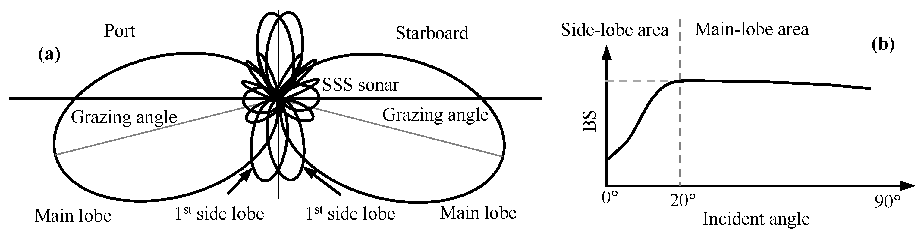
Figure 3.
(a) angular response (AR) effect on side scan sonar (SSS) backscatter with different sediments; and (b) combined effects of the beam pattern and angular response on SSS backscatter.
Figure 3.
(a) angular response (AR) effect on side scan sonar (SSS) backscatter with different sediments; and (b) combined effects of the beam pattern and angular response on SSS backscatter.
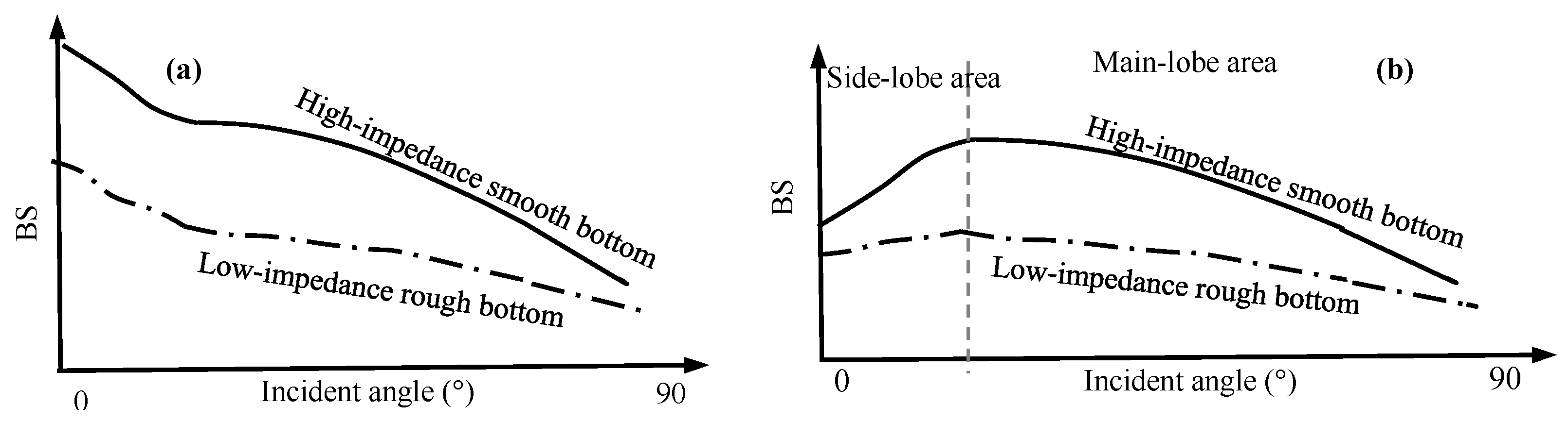
Figure 4.
Flow chart of radiometric distortion correction in SSS data.
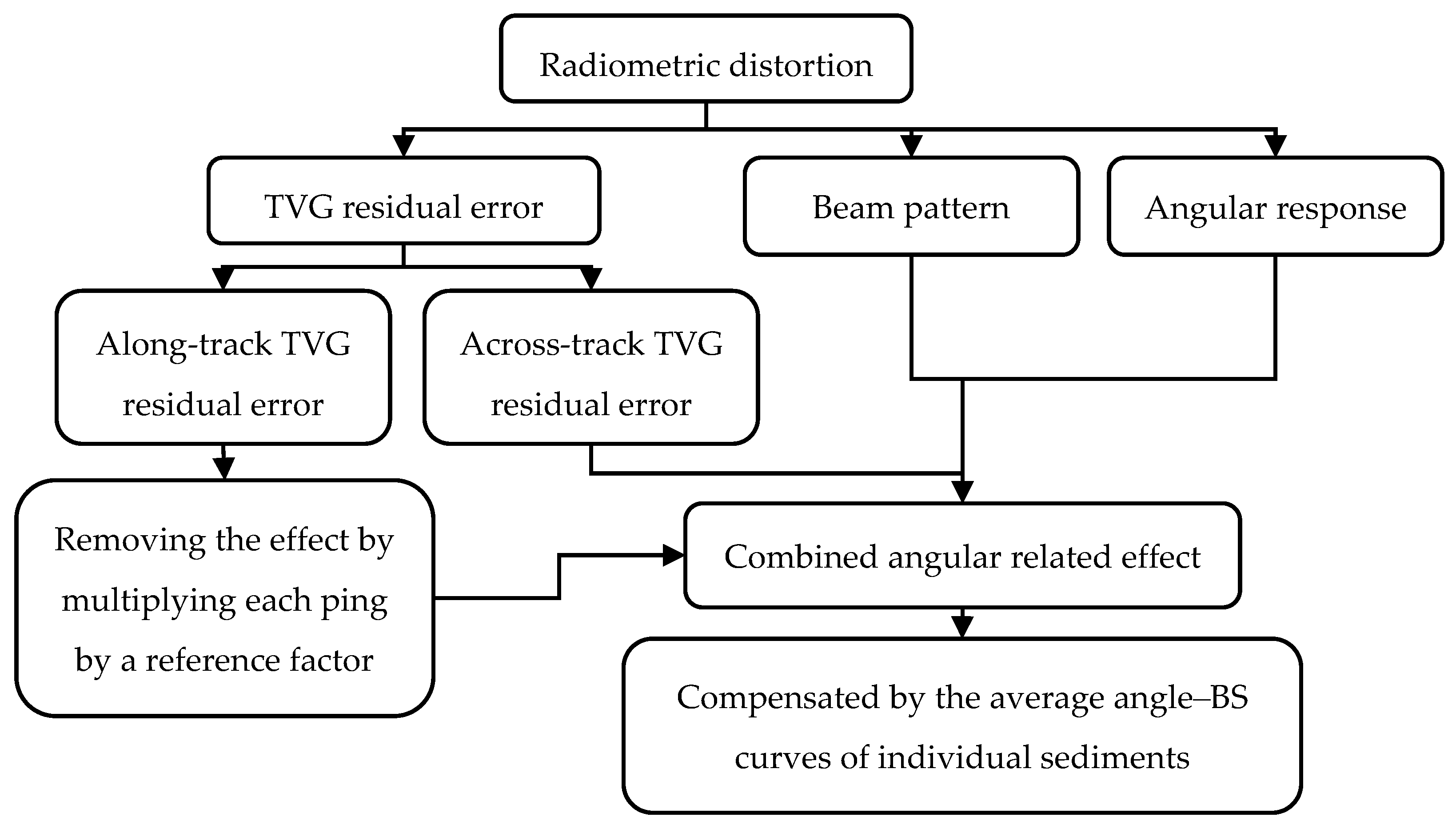
Figure 5.
Bottom tracking and correction of along-track TVG residuals: (a) raw waterfall image; (b) sonar altitudes tracked along the survey line; (c) raw and corrected BS sequences with an incidence angle of 40°; and (d) waterfall image after the removal of the water column and correction (φ denotes the incident angle).

Figure 6.
(a) Range–BS sequence; and (b) corresponding angle–BS sequence of a ping.

Figure 7.
(a) Along-track BS sequences of different incident angles; and (b) their z-score sequences.
Figure 7.
(a) Along-track BS sequences of different incident angles; and (b) their z-score sequences.

Figure 8.
Raw SSS image (a); normalized z-score image (b); and the classified image (c). φ denotes the incident angle.
Figure 8.
Raw SSS image (a); normalized z-score image (b); and the classified image (c). φ denotes the incident angle.

Figure 9.
Iteration method for determining k and classification results under different given values of initial k (k = 7 (a), 4 (b), 3 (c), and 2 (d)). The red rectangle means that the proportion of these clusters is less than 5%, and the yellow rectangle denotes that the clusters’ center distance is extremely close (less than 5% of the BS variation range) and should be merged. φ denotes the incident angle

Figure 10.
Radiometric correction with the proposed method: (a) raw SSS waterfall image; (b) corresponding classification image for k = 3; (c) three angle–BS curves of the three sediment clusters; (d,e) BS sequences of a ping before and after radiometric correction, respectively; and (f) new image after radiometric correction.
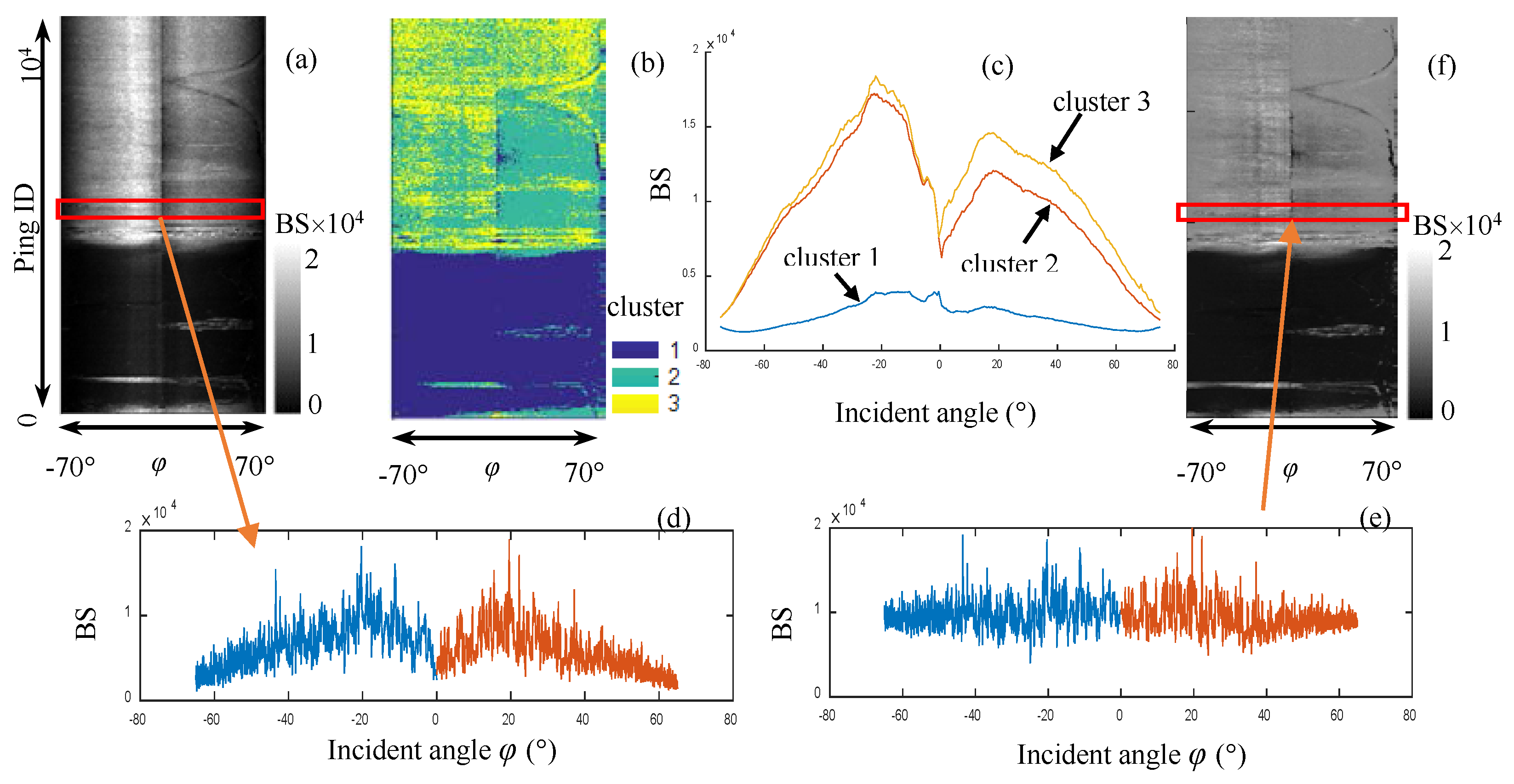
Figure 11.
Comparisons of different radiometric corrections. φ denotes the incident angle: (a) raw SSS image; (b,c) results corrected by the average angle–BS curves of the entire line and every 50 pings, respectively; and (d) result corrected with the proposed method. The red ellipse denotes the sediment transition region, and the yellow rectangle shows the micro sediment variation.
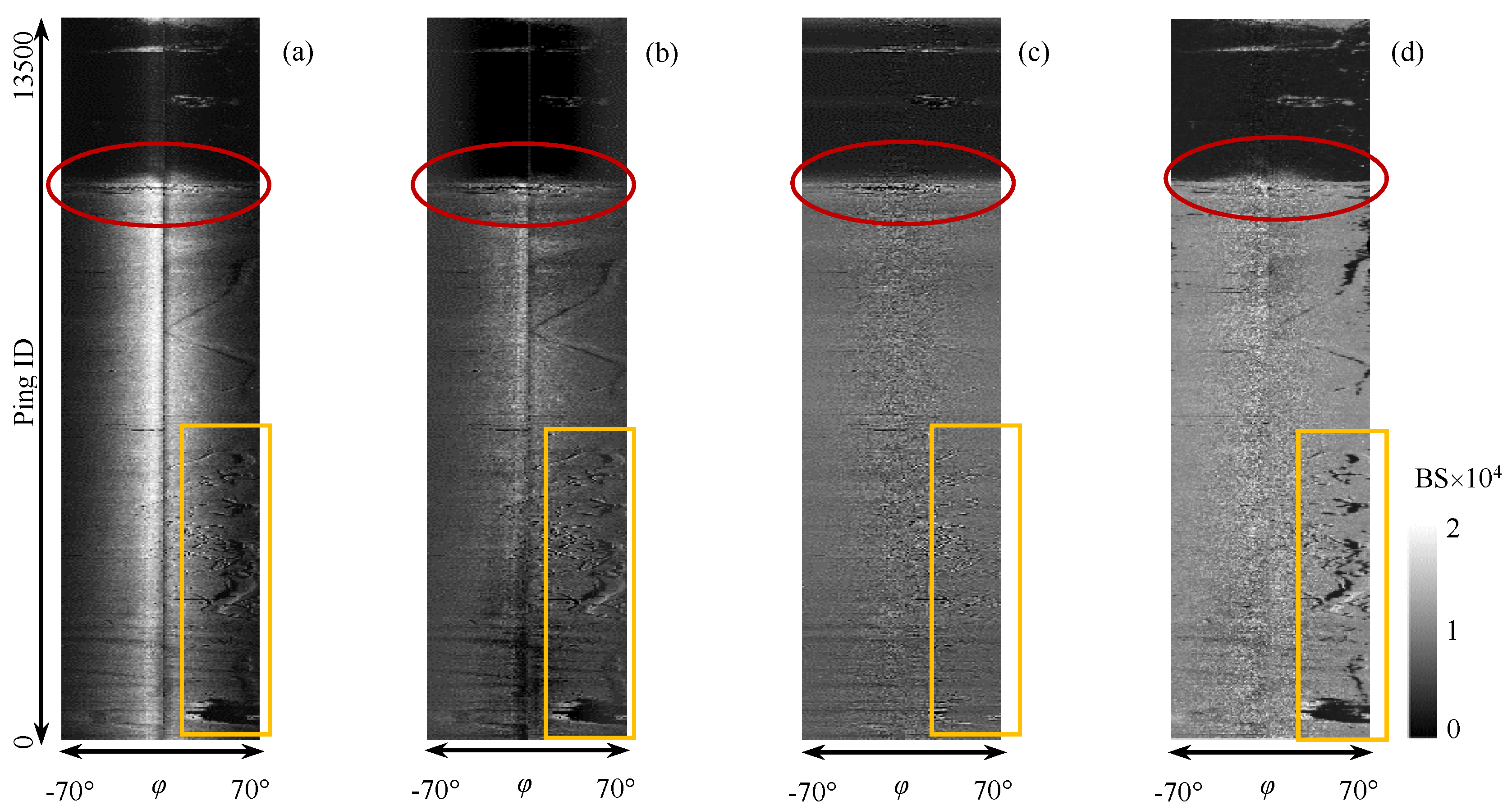
Figure 12.
(a,b) Histograms of the raw BSs and those corrected with the proposed method.
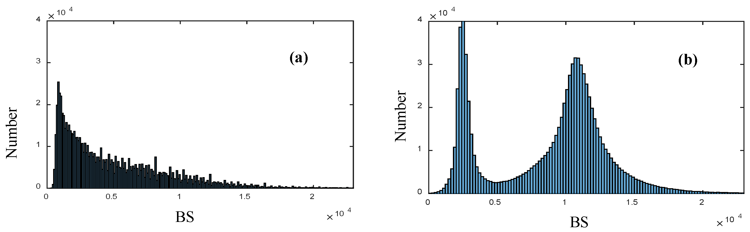
Figure 13.
Radiometric correction of SSS image with various sediments: (a) raw SSS waterfall image; (b) angular waterfall image; (c) sediment classification image; (d) average angle–BS curves of the six sediments; and (e) new image after radiometric correction. φ in (b,c) denotes the incident angle.

Figure 14.
Comparison of raw and corrected sonar images of the entire seabed: (a) raw sonar image; and (b) image corrected with the proposed method. X and Y are the location coordinates projected using universal transverse Mercator projection in Zone 50.
Figure 14.
Comparison of raw and corrected sonar images of the entire seabed: (a) raw sonar image; and (b) image corrected with the proposed method. X and Y are the location coordinates projected using universal transverse Mercator projection in Zone 50.

Figure 15.
Consistency analysis of sediment variations. Lines A and B are two adjacent SSS lines, and Line AB is their mosaic image. The red rectangle denotes the peach-like shape of sediment distribution, and the blue one shows the shapes and positions of two submarine pipelines. The white lines between pings are caused by data losses. The location coordinates are same as Figure 14.

Figure 16.
Bias distributions and corresponding fitting PDF curves of co-located BS biases of raw, and corrected data using the traditional method and proposed method, respectively. μ and σ denote the mean and standard deviation of the fitting curves, respectively.
Figure 16.
Bias distributions and corresponding fitting PDF curves of co-located BS biases of raw, and corrected data using the traditional method and proposed method, respectively. μ and σ denote the mean and standard deviation of the fitting curves, respectively.
© 2017 by the authors. Licensee MDPI, Basel, Switzerland. This article is an open access article distributed under the terms and conditions of the Creative Commons Attribution (CC BY) license (http://creativecommons.org/licenses/by/4.0/).
Share and Cite
MDPI and ACS Style
Zhao, J.; Yan, J.; Zhang, H.; Meng, J. A New Radiometric Correction Method for Side-Scan Sonar Images in Consideration of Seabed Sediment Variation. Remote Sens. 2017, 9, 575. https://doi.org/10.3390/rs9060575
AMA Style
Zhao J, Yan J, Zhang H, Meng J. A New Radiometric Correction Method for Side-Scan Sonar Images in Consideration of Seabed Sediment Variation. Remote Sensing. 2017; 9(6):575. https://doi.org/10.3390/rs9060575
Chicago/Turabian StyleZhao, Jianhu, Jun Yan, Hongmei Zhang, and Junxia Meng. 2017. "A New Radiometric Correction Method for Side-Scan Sonar Images in Consideration of Seabed Sediment Variation" Remote Sensing 9, no. 6: 575. https://doi.org/10.3390/rs9060575
Note that from the first issue of 2016, this journal uses article numbers instead of page numbers. See further details here.