
Mapping Spartina alterniflora Biomass Using LiDAR and Hyperspectral Data


1
School of Resource and Environmental Sciences, Wuhan University, Wuhan 430079, China
2
Chinese Academy of Surveying and Mapping, Beijing 100830, China
3
The Fourth Institute of Anhui Surveying and Mapping, Hefei 230031, China
*
Authors to whom correspondence should be addressed.
Remote Sens. 2017, 9(6), 589; https://doi.org/10.3390/rs9060589
Submission received: 19 April 2017
/
Revised: 28 May 2017
/
Accepted: 7 June 2017
/
Published: 10 June 2017
(This article belongs to the Special Issue Fusion of LiDAR Point Clouds and Optical Images)
Abstract
:Large-scale coastal reclamation has caused significant changes in Spartina alterniflora (S. alterniflora) distribution in coastal regions of China. However, few studies have focused on estimation of the wetland vegetation biomass, especially of S. alterniflora, in coastal regions using LiDAR and hyperspectral data. In this study, the applicability of LiDAR and hypersectral data for estimating S. alterniflora biomass and mapping its distribution in coastal regions of China was explored to attempt problems of wetland vegetation biomass estimation caused by different vegetation types and different canopy height. Results showed that the highest correlation coefficient with S. alterniflora biomass was vegetation canopy height (0.817), followed by Normalized Difference Vegetation Index (NDVI) (0.635), Atmospherically Resistant Vegetation Index (ARVI) (0.631), Visible Atmospherically Resistant Index (VARI) (0.599), and Ratio Vegetation Index (RVI) (0.520). A multivariate linear estimation model of S. alterniflora biomass using a variable backward elimination method was developed with R squared coefficient of 0.902 and the residual predictive deviation (RPD) of 2.62. The model accuracy of S. alterniflora biomass was higher than that of wetland vegetation for mixed vegetation types because it improved the estimation accuracy caused by differences in spectral features and canopy heights of different kinds of wetland vegetation. The result indicated that estimated S. alterniflora biomass was in agreement with the field survey result. Owing to its basis in the fusion of LiDAR data and hyperspectral data, the proposed method provides an advantage for S. alterniflora mapping. The integration of high spatial resolution hyperspectral imagery and LiDAR data derived canopy height had significantly improved the accuracy of mapping S. alterniflora biomass.
1. Introduction
Spartina alterniflora (S. alterniflora) is a perennial deciduous grass which is found in intertidal wetlands, especially estuarine salt marshes. Some biologists and geographers have conducted various researches on ecological characteristics of S. alterniflora and its impacts on environment [1,2,3,4,5,6,7]. In recent years, some evidence has been reported that S. alterniflora could compete with native plants, threaten native ecosystems and coastal aquaculture, and cause declines in local biodiversity [2,3,4]. In invasive studies research, the invasion and control of S. alterniflora has been important and drawn attention in China and abroad [1,5]. In China, S. alterniflora is widely distributed along the eastern coastal region of China from Tianjin to Beihai, with a concentration in Jiangsu Province. Large-scale coastal reclamation has resulted in significant changes in distribution of S. alterniflora in Dafeng coastal zone of Jiangsu. The formation, expansion, and distribution of the plant in Jiangsu coastal zone has been studied [4,6,7]. However, no data have been published on the spatial-temporal distribution and biomass of S. alterniflora in Dafeng because of the difficulty in accessing salt marshes using traditional biomass measurement methods and observation estimation methods.
Remote sensing data, such as optical remote sensing images, aerial images, radar data and LiDAR point cloud data, have been widely used in wetland vegetation classification, information extraction of canopy structure characteristics, and vegetation biomass estimation. However, these investigations generally focused on horizontal surface information of vegetation, because optical signals cannot penetrate the upper vegetation or other sheltered features, and Synthetic Aperture Radar (SAR) could be disturbed by the topographic relief and no longer sensitive when the biomass was very high, which restricted its application in regional estimation [8,9,10,11,12,13,14]. Developments of LiDAR technology have enabled penetration of the high density vegetation canopy to obtain accurate and detailed vegetation structure parameters. Many studies have attempted to estimate wetland vegetation biomass and extract information of forest canopy structure characteristics using LiDAR data [11,12,15,16,17,18,19]. Moreover, several studies also focused on wetland vegetation biomass estimation using SAR data, CBERS images, fusion of Landsat TM and ENVISAT ASAR, etc. [20,21]. Long-term monitoring of biophysical characteristics of tidal wetlands using MODIS was also studied [22]. Recently, some studies focused on estimating forest vegetation, crop biomass, leaf nitrogen content, and land cover mapping using fusion data of hypersectral and LiDAR data. They showed its advantage for producing better results than hyperspectral images or LiDAR data [23,24,25,26,27], such as on tropical forest biomass [28], forest canopy height and biomass [10], maize biomass [29], and crop species classification [30]. Using LiDAR, hyperspectral and radar data, some researchers have discriminated some wetland species and made efforts on estimation of wetland biomass, water content and leaf area index (LAI) [31,32]. The integration of hyperspectral imagery and LiDAR derived elevation data for mapping salt marsh vegetation has also been studied [33]. In these studies, biomass estimation for multiple types of wetland vegetation used to based on differentiation of vegetation types with coverage. For S. alterniflora research, O’Donnell ever examined the influence of abiotic drivers on its biomass using Landsat 5 satellite imagery [34]. However, there have been some estimation problems of wetland vegetation biomass caused by different vegetation types and by different canopy height. Few studies have focused on estimating wetland vegetation biomass, especially S. alterniflora, in coastal regions using high spatial resolution hyperspectral image and LiDAR data. The objective of this study was to explore the applicability of LiDAR and hypersectral data for estimating S. alterniflora biomass and mapping its distribution in coastal regions in China.
2. Materials and Methods
2.1. Study Area
The study area was in Dafeng County in Jiangsu coastal region of China (latitude from 32°56′ to 33°36′ N, and longitude from 120°13′ to 120°56′ E). The Dafeng coast comprises a typical silt mud plain coast with a 112-km coastline and more than 1000 km2 of coastal tidal flats. It is one of regions in China with the most abundant coastal tidal flat resources and frequent beach reclamation activities (Figure 1). S. alterniflora was introduced in Dongtai, Jiangsu in 1988 and spread to the north along the coast. A large amount of S. alterniflora were distributed in Dafeng coastal tidal flats over the past few decades.
2.2. Data Collection
Hyperspectral data with 0.78 m spatial resolution, airborne LiDAR data with ground spot diameter less than and equal to 0.6 m, and aerial image with 0.14 m spatial resolution were acquired by a Cessna 208B multipurpose aircraft in November 2014. It covered a ground area of approximately 20 km2. This multipurpose aircraft was equipped with an airborne hyperspectral scanner (Finland SPECIM AISA EAGLE II), aerial digital camera (Hasselblad H4D), and airborne laser radar system (Austria RIEGL LMS Q-680i).
The airborne LiDAR data obtained by RIEGL LMS Q-680i was echo data with a 1550 nm laser wavelength and a 200 KHz pulse repetition frequency in the airborne radar system. Hyperspectral data with a 0.78 m spatial resolution by SPECIM AISA EAGLE II was acquired as 400–970 nm visible/near infrared data with all 64 bands. The three-dimensional structures of the respective LiDAR and hyperspectral data, as well as detailed two-dimensional spectral information, were used in the study.
2.3. Collection of Vegetation Samples and Spectra
Numerous field surveys and experimental studies on wetland vegetation in the Dafeng County study area were performed. Fifty-four vegetation samples were collected in November 2014. Sampling sites were positioned by a Trimble Pro XRR global positioning system (GPS) unit. The vegetation samples were 1 m × 1 m in size (vegetation cover > 20%) and 3 m × 3 m (vegetation cover ≤ 20%). Because when the average coverage of a vegetation sample is less than or equal to 20%, that means the vegetation is too sparse, artificial error of collecting vegetation sample could be larger using 1 m × 1 m sample. Vegetation types included reed, Artemisia halodendron (A. halodendron), and S. alterniflora. Vegetation sample biomass was collected and weighed. Reflectance spectra of these vegetation samples were measured in the field and in the laboratory at 1 m above the soil and vegetation surface with an 8% field of view both using a high spectral resolution analytical spectral device (ASD), respectively. ASD operates in visible, near infrared and shortwave infrared bands (350–2500 nm). A reference panel by Labsphere Incorporated, Sutton, New Hampshire was used as reference before and after each measurement. Six individual spectra were averaged for each measured sample.
2.4. Data Pre-Processing
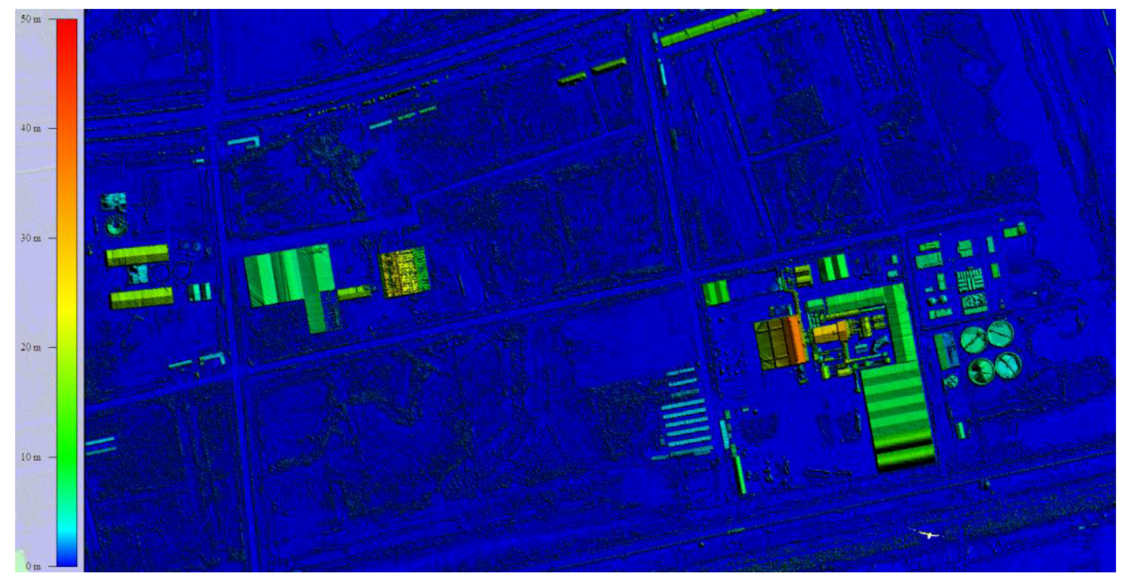
Airborne LiDAR dada were pre-processed through multi-strip stitching, singular-point deletion, and point-cloud filtering pre-processing under the Terrasolid platform. The canopy height mode was used to generate and extract vegetation height information. Figure 2 depicts the classification results of the LiDAR point cloud data. The images of the digital elevation model (DEM) and digital surface model (DSM) were created through pre-processing of point cloud filtering. Figure 3 is the DSM result extracted from point cloud data.
The preprocessing process for hyperspectral image data, including mosaic, radiation calibration, geometric correction was handled by data producer. The point cloud data of LiDAR system is three-dimensional data, while hyperspectral image data is two-dimensional flat surface data. If directly registration is done for the two kinds of data, more complex algorithms and data processing processes could be needed. It was not the focus of this study. The study was only to extract vegetation canopy height information from point cloud data. The geometric correction and registration of hyperspectral images were performed based on ground-control points (ten ground-control points) and DEM from point cloud data in order to have the same geographical coordinates, the same spatial resolution. The relative geometric correction residual error was 0.827 pixels. Atmospheric correction of hyperspectral images was conducted using the ENVI Fast Line-of-sight Atmospheric Analysis of Hypercubes (FLAASH) modular in ENVI 5.3.1 software (Exelis Visual Information Solutions Corporation, USA). The image data were converted to relative reflectance using the internal average relative reflectance for image calibration. Resampling was carried out using the nearest neighbor method in order to not severely alter the pixel values.
2.5. Biomass Estimation Model
Multivariate statistical analysis was conducted on vegetation biomass and spectral data using SPSS 17 software (International Business Machines Corporation, USA). Nonparametric test methods such as one-sample K-S test method were employed for normal distribution analysis. Correlation using Pearson correlation coefficient between measured vegetation parameters and absorption feature at the obtained wavelength, as well as the vegetation index, were calculated in SPSS software. The Pearson correlation coefficient is calculated by dividing the covariance by the standard deviation of two variables. Multi-regression analysis between spectral reflectance and associated vegetation parameters were conducted.
In this study, according to the classification of wetland vegetation types, two types of biomass estimation models were respectively established to reduce estimation error caused by different vegetation types. Thus, these two types of biomass estimation models were analyzed and compared. One focused on a single type of vegetation, S. alterniflora. Another focused on all types of wetland vegetation as a whole, including reeds, A. halodendron, and S. alterniflora. Eighteen S. alterniflora samples and fifty-four wetland vegetation samples were randomly divided into two groups. One group was used for developing the model (up to 70% of the total number of samples); the other was used for validation (up to 30% of the total number of samples). Taking into account the practicality of the experiment, a multiple linear regression model (MLR) was used to develop the biomass estimation model of vegetation.
Firstly, the spectral absorption features of wetland vegetation were analyzed. There were sensitive absorption features at blue band (452 nm), green band (534 nm), red band (694 nm) and near infrared band (865 nm) for wetland vegetation. So the correlation coefficients of spectral reflectance at these four wavelengths and biomass content of wetland vegetation and S. alterniflora were analyzed. Vegetation indexes derived from hyperspectral images were also used as indicators of vegetation performance. Ten kinds of vegetation indexes including RVI (Ratio Vegetation Index) [35], NDVI (Normalized Difference Vegetation Index) [36], GNDVI (Green Normalized Difference Vegetation Index) [37], DVI (Difference Vegetation Index) [38], RDVI (Ratio Difference Vegetation Index) [39], TVI (Transformed Vegetation Index) [40], VARI (Visible Atmospherically Resistant Index) [41], ARVI (Atmospherically Resistant Vegetation Index) [42], GEMI (Global Environment Monitoring Index) [43]) and EVI (Environment Vegetation Index) [44] were calculated from hyperspectral spectral bands (Figure 4), and vegetation canopy height was also derived from LiDAR data. The correlation coefficients of above ten kinds of vegetation indexes and vegetation canopy height with biomass content of wetland vegetation and S. alterniflora were also analyzed.
Secondly, the variables with high correlation coefficient with biomass content were used as independent variables of biomass estimation model. In the study, the spectral reflectance at wavelengths of 452 nm, 534 nm, 694 nm and 865 nm, and ten kinds of vegetation indexes derived from hyperspectral images could be as independent variables of biomass estimation model. Vegetation canopy height derived from airborne LiDAR point cloud data was introduced into the biomass estimation model. The biomass estimation model of vegetation employed a multiple linear regression model (MLR).
The detailed multiple linear regression model equation is:
where Y is the vegetation biomass (wet weight), and X denotes the spectral reflectance at wavelengths of 452 nm, 534 nm,694 nm and 865 nm, vegetation indexes, and vegetation canopy height. In addition, b is the regression model constant, and a is the coefficient of the independent variables of X.
Y = b + a1X1 + a2X2 + a3X3 +…+ anXn
At last, the reliability and accuracy of biomass estimation models were conducted using measured sample data in the field. In the study, R squared coefficient, root mean square error (RMSE) value, the residual predictive deviation (RPD) (the ratio of standard deviation to RMSE) [45] and the estimation error (p value) were used as assessment indicators of biomass estimation models.
3. Results and Discussion
3.1. Biomass Estimation Model of Wetland Vegetation
A comparative experiment was conducted for evaluating the biomass estimation accuracy. One included reeds, A. halodendron, and S. alterniflora in the study area for multivariate statistical analysis. The other included only S. alterniflora for multivariate statistical analysis.
Correlation analysis between spectra reflectance in field and biomass content (wet weight) of wetland vegetation samples was conducted (Table 1). Results showed that correlation coefficients were higher at a wavelength of 452 nm (blue), 534 nm (green), 694 nm (red), and 865 nm (near infrared). The correlation analysis between the biomass content and vegetation indexes (RVI, NDVI, GNDVI, DVI, RDVI, EVI, TVI, GEMI, VARI, ARVI, and vegetation canopy height) was also performed (Table 1). The above correlation coefficients were significant at α = 0.05 level. The biomass content was significantly correlated with the following parameters: the reflectance at a wavelength of 534 nm (0.639), 865 nm (0.546), and 452 nm (0.515); GEMI (0.507), TVI (0.506), and DVI (0.488); and vegetation canopy height (0.421).
The vegetation parameters with correlation coefficients greater than 0.5 were chosen as independent variables in the wetland vegetation estimation model. R534 (x1), R865 (x2), R452 (x3), GEMI (x4), and TVI (x5) were introduced in the wetland vegetation biomass estimation model. The different multivariate statistical models using four types of variable introduction methods are listed in Table 2.
As shown in Table 2, the model using the stepwise regression method by variable forward entry has the highest R squared coefficient and lowest estimation error p value. Therefore, it was chosen to estimate the biomass content of the wetland vegetation. This regression model was significant at α = 0.05, where α is the significance level. The regression model could be formulated as:
where Y is the biomass content of the wetland vegetation, X1 is the band reflectance at 534 nm, X5 is vegetation index TVI, the R squared coefficient is 0.704, and the root mean square error value (RMSE) is 0.24.
Y = 35.411X1 + 0.124X5 − 1.228
3.2. Biomass Estimation Model of Spartian Alterniflora
To overcome the disadvantages of the obvious differences in spectral features and canopy heights of reeds, A. halodendron, and S. alterniflora for the wetland vegetation estimation model, an estimation model for S. alterniflora is proposed. The correlation between S. alterniflora spectra reflectance and biomass content (wet weight) of S. alterniflora samples was analyzed (Table 3). The results showed that correlation coefficients between the biomass content of S. alterniflora and spectral reflectance were higher at wavelengths of 452 nm (blue), 534 nm (green), 694 nm (red), and 865 nm (near infrared). Correlation coefficients of S. alterniflora biomass content were also higher with RVI, NDVI, GNDVI, DVI, RDVI, EVI, TVI, VARI, ARVI, and vegetation height. The above correlation coefficients were significant at α = 0.05 level. The correlation coefficient values decreased in the following order: vegetation canopy height (0.817), NDVI (0.635), ARVI (0.631), VARI (0.599), and RVI (0.520). These correlations were statistically significant at α = 0.05 significance level. The vegetation canopy height derived from LiDAR data was highly correlated with the biomass content of S. alterniflora with the highest correlation coefficient of 0.817, while it was less correlated with wetland vegetation in the above analysis (0.421).
The vegetation parameters with correlation coefficients that was greater than 0.5 were chosen as independent variables for the S. alterniflora biomass estimation model. Thus, the vegetation canopy height (x1), NDVI (x2), ARVI (x3), VARI (x4), and RVI (x5) were introduced in a multivariate statistical analysis for developing the model. Different multivariate statistical models using four types of variable introduction methods were developed (Table 4).
As shown in Table 4, the model using the stepwise regression method by variable backward elimination is characterized by the highest R squared coefficient and lowest p value. Thus, it was chosen to estimate the biomass content of S. alterniflora. This regression model was statistically significant at α = 0.05 level with R squared coefficient of 0.902. The regression model could be formulated as:
where Y is the S. alterniflora biomass content, X1 is the vegetation height, X4 is VARI, the R squared coefficient is 0.902, and the RMSE is 0.15.
Y = 0.514X1 + 1.11X4 + 0.388
The vegetation canopy height showed significant effects on the biomass estimation models of S. alterniflora using LiDAR and hyperspectral data with high spatial resolution. On the other hand, the reflectance at wavelengths of R534, R865, and R452 had a significant effect on the estimation model of the wetland vegetation in the study area. The results further demonstrated the importance of vegetation canopy variables, such as vegetation height, as a major factor affecting the S. alterniflora biomass distribution. Vegetation canopy variables should be introduced into estimation models of vegetation biomass using remote sensing images. The results also implied that the fusion of LiDAR and hyperspectral data can improve the accuracy of vegetation biomass estimation using remote sensing techniques.
3.3. Model Accuracy Verification
Reliability and accuracy of biomass estimation models should be assessed for mapping biomasses of different types of vegetation using hyperspectral images and airborne LiDAR data. Two types of biomass estimation models for S. alterniflora and wetland vegetation were respectively verified using the same measured sample data in the field. The R squared coefficient (R2), root mean square error (RMSE) value, the residual predictive deviation (RPD) and the estimation error (p value) were used as assessment indicators of biomass estimation models. Results indicated that the estimation error of wetland vegetation was up to 36.14%, whereas that of S. alterniflora was 10.55%. The RMSE value of estimation model for S. alterniflora was 0.15, which was much lower than that of wetland vegetation (0.24). The RPD value of estimation model for S. alterniflora and wetland vegetation was both more than 2.0. The result indicated S. alterniflora was readily estimated (R2 = 0.902, RPD = 2.62). Estimation accuracy of S. alterniflora for a single type of vegetation was higher than that of wetland vegetation for mixed vegetation types. The predicted biomass content of S. alterniflora using the stepwise regression model by the variable backward elimination method showed a linear distribution with test biomass content (Figure 5).
Many obvious differences exist in spectral features and canopy heights of reeds, A. halodendron, and S. alterniflora. These differences may be due to the estimation accuracy of wetland vegetation biomass model being relatively lower on account of large differences of independent variables. Results showed that the proposed estimation model of vegetation biomass based on vegetation classification in coastal regions was beneficial to improving its accuracy by fusing airborne LiDAR and hyperspectral data.
3.4. Mapping the S. alternniflora Biomass Distribution
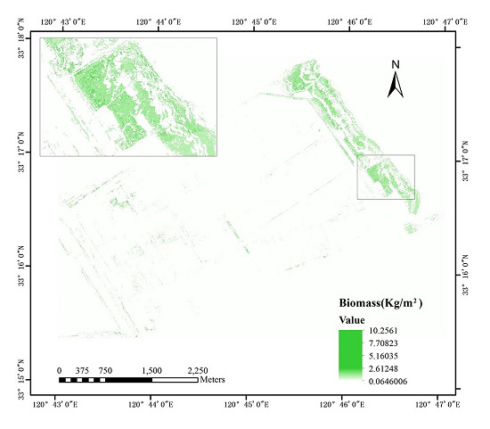
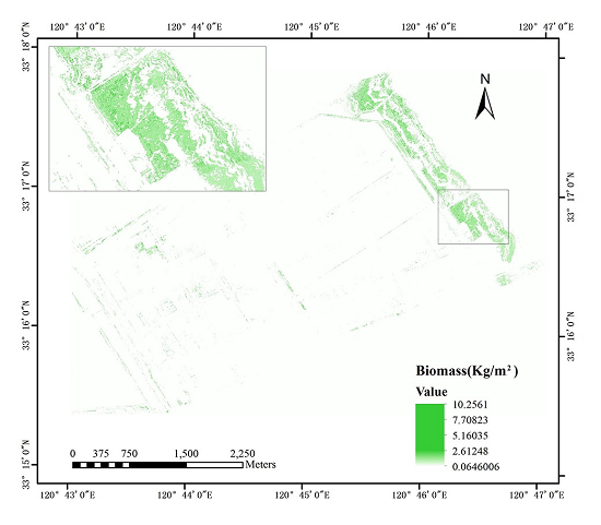
The classification map of reeds, A. halodendron, and S. alterniflora was derived from high spatial resolution images with a 0.14-m resolution in the study area. Distribution information of S. alterniflora was extracted from hyperspectral images by mask processing. The processed hyperspectral image was used to map the distribution of S. alterniflora biomass using the stepwise regression model (Figure 6). Results indicated that most S. alterniflora were continuously distributed and clustered together in the coastline region, whereas others were primarily scattered within the inland region of the study area. S. alterniflora flourished with a higher vegetation density in the coastline region. There were few differences in the growth status of S. alterniflora in the study area. Statistical analysis on the pixel number for the S. alterniflora estimated biomass showed that the number of pixels with biomass distribution between 0 and 15.63 kg/m2 was the largest and very concentrated. That is, the estimated biomass of S. alterniflora occurred within this range. Based on the known biomass values of individual pixels and the number of pixels, the total biomass of S. alterniflora was estimated to be up to 681.18 t, or 6.88 t per hectare in the study area. The distribution of biomass content for S. alterniflora is in agreement with the field survey results and the decreasing trend from the coastline to the inland area of Dafeng County.
As most of wetland vegetation types in the mature period, its growth density is large, the vegetation biomass estimation using ordinary hyperspectral image has been unable to meet the research accuracy requirements. Under the same vegetation coverage and the same canopy height, the biomass of different vegetation types is different, and under the same vegetation coverage and the same vegetation type, the biomass of vegetation at different heights is also different. The study for mapping S. alternniflora biomass using high spatial resolution hyperspectral image and LiDAR data was to overcome the intertype error (caused by different vegetation types) and error of height difference (caused by different canopy height). It is consistent with Klemas’s result that the integration of hyperspectral imagery and LiDAR derived elevation data has also significantly improved the accuracy of mapping salt marsh vegetation [33]. The ability of the method to estimate the S. alternniflora biomass may be due to correlations with vegetation properties having a response in blue, green, red, near infrared bands and vegetation indexes and vegetation canopy height using linear regression model. Many studies indicated vegetation properties have a primary response in the 400–970 nm visible/near infrared light region. Developing regression models of S. alternniflora biomass estimation for each one of the sixty-four spectral bands or determining sensitive bands using other regression models such as partial least square regression (PLSR) should be discussed in future. On the other hand, the above estimation accuracy may be improved due to the inability of the linear regression models to accurately represent the relationship between the biomass of S. alternniflora and wetland vegetation, and/or that other vegetation properties not measured may influence the spectra.
Furthermore, the biomass estimation method using fusion of LiDAR data and hyperspectral data provides an advantage for S. alterniflora mapping. This method combines spectral and texture information of vegetation derived from hyperspectral images, canopy information derived from LiDAR data, vegetation types derived from high spatial resolution images, and field survey information. This result is consistent with research results on maize biomass estimation by Wang et al. [29], mapping biomass and stress by Swatantran et al. [24], crop species classification by Liu et al. on [30], estimation of above ground biomass for moist forest by Vaglio et al. [25]. It is significant for rapid monitoring of vegetation situation using multi-source data. It can therefore notably contribute to ecosystem management by providing a tool for remotely monitoring vegetation parameters at a regional scale. Although the distribution of estimated biomass content for S. alterniflora with LiDAR and hyperspectral data had only a spatial variation in the study area, the method is less time-consuming and more cost-effective than traditional methods. The latter methods on a regional scale require a large number of vegetation samples on account of the high spatial heterogeneity of vegetation. Hence, this study provides an advanced method compared to traditional vegetation surveys.
Nevertheless, some issues should be identified for mapping S. alterniflora biomass content at regional scale. Hyperspectral data and airborne LiDAR data directly acquired by aircraft may be affected by natural surface conditions, atmosphere, and illumination conditions. These impacts will be finely identified and corrected using ample reference data in the field, which will be combined with ancillary data. The adoption of this estimation method may be promising in operational terms, while the accuracy of mapping S. alterniflora biomass content should be further improved.
4. Conclusions
Biomass content of wetland vegetation, including reeds, A. halodendron, and S. alterniflora as a whole, as well as the single type of S. alterniflora, were estimated in this study using a multivariate statistical method using hyperspectral image and LiDAR data. Correlation coefficients of wetland vegetation biomass with spectral reflectance at wavelengths of R534 (0.639), R865 (0.546) and R452 (0.515), and vegetation indices of GEMI (0.507), TVI (0.506) and DVI (0.488), and vegetation canopy height (0.421) were higher than other variables. The multivariate regression model of wetland vegetation using the variable forward enter method with R squared coefficient of 0.704 was proposed to estimate biomass content of wetland vegetation.
To overcome the disadvantages of differences in spectral features and canopy heights of wetland vegetation, S. alterniflora estimation model was proposed. Correlation analysis results showed that the highest correlation coefficient was 0.817 for vegetation canopy height, followed by NDVI (0.635), ARVI (0.631), VARI (0.599), and RVI (0.520). The estimation model using the variable backward elimination method with R squared coefficient of 0.902 was proposed to estimate the S. alterniflora biomass. Estimation accuracy of S. alterniflora for a single type of vegetation was higher than that of wetland vegetation for mixed vegetation types. The predicted biomass of S. alterniflora showed a linear distribution with test biomass. The total S. alterniflora biomass was estimated to 6.88 t per hectare in the study area. The distribution of S. alterniflora biomass is in agreement with the field survey results from Dafeng County.
This study demonstrated that the vegetation canopy height variable should be introduced into vegetation biomass estimation models, which can improve the estimation accuracy. Furthermore, the proposed estimation model of vegetation biomass based on vegetation classification was beneficial to improving its accuracy using the fusion of LiDAR and hyperspectral data. Mapping S. alternniflora biomass using high spatial resolution hyperspectral image and LiDAR data could improve the estimation error caused by different vegetation types and different canopy height. It is advantageous for S. alterniflora mapping, compared to traditional survey. This research thus significantly contributes to ecosystem management by providing a tool for remotely monitoring vegetation parameters at regional scale. However, the impacts of natural surface conditions, atmosphere, and illumination conditions should be further studied for mapping S. alterniflora biomass content. Moreover, the mapping accuracy of S. alterniflora biomass should be further improved.
Acknowledgments
The authors acknowledge financial support from the National Natural Science Foundation of China (41330750) and the project of high-level talents import plan in Wuhan University.
Author Contributions
Jing Wang is the principal author that provided the overall conception of the study and wrote the majority of the manuscript; Zhengjun Liu conceived and designed the experiments and contributed in the methods design; Haiying Yu contributed in data analysis and study experiments and wrote the part of the manuscript; Fangfang Li helped to analyze the data and revise the manuscript figures. The order of the authors reflects their levels of contribution.
Conflicts of Interest
The authors declare no conflict of interest.
References
- Shen, Y.M.; Yang, J.S.; Zeng, H.; Zhou, Q. Review of studies on alien species Spartina alterniflora in China. Mar. Environ. Sci. 2008, 27, 391–396. [Google Scholar]
- Brusati, E.D.; Grosholza, E.D. Effect of native and invasive cordgrass on Macoma petalum density, growth, and isotopic signatures. Estuar. Coast. Shelf Sci. 2007, 71, 517–522. [Google Scholar] [CrossRef]
- Rosso, P.H.; Ustin, S.L.; Hastings, A. Use of lidar to study changes associated with Spartina invasion in San Francisco Bay marshes. Remote Sens. Environ. 2006, 100, 295–306. [Google Scholar] [CrossRef]
- Zhu, D.; Gao, S. The expansion of Spartina alterniflora marsh in response to tidal flat reclamation, central Jiangsu coast, eastern China. Geogr. Res. 2014, 33, 2382–2392. (In Chinese) [Google Scholar]
- Thomas, M.B.; Reid, A.M. Are exotic natural enemies an effective way of controlling invasive plants? Trends Ecol. Evol. 2007, 22, 447–453. [Google Scholar] [CrossRef] [PubMed]
- Zhang, R.S.; Shen, Y.M.; Lu, L.Y.; Yan, S.G.; Wang, Y.H.; Li, J.L.; Zhang, Z.L. Formation of Spartina alterniflora salt marshes on the coast of Jiangsu Province, China. Ecol. Eng. 2004, 23, 95–105. (In Chinese) [Google Scholar] [CrossRef]
- Liu, C.Y.; Zhang, S.Q.; Jiang, H.X.; Wang, H. Spatiotemporal dynamics and landscape pattern of alien species Spartina alterniflora in Yancheng coastal wetlands of Jiangsu Province, China. Chin. J. Appl. Ecol. 2009, 20, 901–908. (In Chinese) [Google Scholar]
- Tong, Q.X.; Zheng, L.F.; Wang, J.N. Study on Imaging Spectrometer Remote Sensing Information for Wetland Vegetation. J. Remote Sens. 1997, 1, 50–57. (In Chinese) [Google Scholar]
- Fu, X.; Liu, G.H.; Huang, C.; Liu, Q.S. Remote sensing estimation models of Suaeda salsa biomass in the coastal wetland. Acta Ecol. Sin. 2012, 32, 5355–5362. [Google Scholar]
- Tang, X.G. Estimation of Forest Aboveground Biomass by Integrating ICESat/GLAS Waveform and TM Data. Doctoral Dissertation, University of Chinese Academy of Sciences, Beijing, China, 2013. [Google Scholar]
- Kasischke, E.S.; Bourgeau-Chavez, L.L. Monitoring South Florida wetlands using ERS-1 SAR imagery. Photogramm. Eng. Remote Sens. 1997, 63, 281–291. [Google Scholar]
- Temilola, E.F.; Amanda, H. Armstrong Remote Characterization of Biomass Measurements: Case Study of Mangrove Forests; INTECH Open Access Publisher: Rijeka, Croatia, 2010; p. 202. ISBN 978-953-307-113-8.2010. [Google Scholar]
- Rajab Pourrahmati, M.; Baghdadi, N.; Asghar Darvishsefat, A.; Namiranian, M.; Gond, V.; Moeinazad Tehrani, S.M.; Fayad, I.; Bailly, J.S. Capability of GLAS/ICESat data to estimate forest canopy height and volume in mountainous forests of Iran. IEEE J. Sel. Top. Appl. Earth Obs. Remote Sens. 2016, 8, 5246–5261. [Google Scholar] [CrossRef]
- Fayad, I.; Baghdadi, N.; Guitet, S.; Bailly, J.S.; Hérault, B.; Gond, V.; El Hajj, M.; Ho Tong Minh, D. Aboveground biomass mapping in French Guiana by combining remote sensing, forest inventories and environmental data. Int. J Appl. Earth Obs. 2016, 52, 502–514. [Google Scholar] [CrossRef]
- Li, X.; Yeh, G.A.; Wang, S.G.; Liu, K.; Liu, X.P. Estimating Mangrove Wetland Biomass Using Radar Remote Sensing. J. Remote Sens. 2006, 10, 387–396. (In Chinese) [Google Scholar]
- Ceballos, A.; Hernández, J.; Corvalán, P.; Galleguillos, M. Comparison of Airborne LiDAR and Satellite Hyperspectral Remote Sensing to Estimate Vascular Plant Richness in Deciduous Mediterranean Forests of Central Chile. Remote Sens. 2015, 7, 2692–2714. [Google Scholar] [CrossRef]
- Boudreau, J.; Nelson, R.F.; Margolis, H.A.; Beaudoin, A.; Guindon, L.; Kimes, D.S. Regional aboveground forest biomass using airborne and spaceborne LiDAR in QuéBec. Remote Sens. Environ. 2008, 112, 3876–3890. [Google Scholar] [CrossRef]
- Maselli, F.; Chiesi, M.; Montaghi, A.; Pranzini, E. Use of ETM+ images to extend stem volume estimates obtained from LiDAR data. ISPRS J. Photogramm. 2011, 66, 662–671. [Google Scholar] [CrossRef]
- Li, J.Q. Method for Extracting Lower Vegetation Structure of Forest Canopy Using LiDAR Data. Doctoral Dissertation, Tsinghua University, Beijing, China, 2011. (In Chinese). [Google Scholar]
- Wang, Q.; Liao, J.J. Estimation of Wetland Vegetation Biomass in the Poyang Lake Area Using Landsat TM and ENVISAT ASAR Data. J. Geoinf. Sci. 2010, 12, 282–291. (In Chinese) [Google Scholar] [CrossRef]
- Tan, Q.M.; Liu, Y.H.; Zhang, H.B. Classification of vegetation coverage of wetland landscape based on remote sensing in coastal area in Jiangsu province. Remote Sens. Technol. Appl. 2013, 28, 934–940. (In Chinese) [Google Scholar]
- Ghosh, S.; Mishra, D.R.; Gitelson, A.A. Long-term monitoring of biophysical characteristics of tidal wetlands in the northern Gulf of Mexico—A methodological approach using MODIS. Remote Sens. Environ. 2016, 173, 39–58. [Google Scholar] [CrossRef]
- Streutker, D.R.; Mundt, J.T.; Glenn, N.F. Mapping Sagebrush Distribution Using Fusion of Hyperspectral and LiDAR Classifications. Photogramm. Eng. Remote Sens. 2006, 72, 47–54. [Google Scholar]
- Swatantran, A.; Dubayah, R.; Roberts, D.; Hofton, M.; Blair, J.B. Mapping biomass and stress in the Sierra Nevada using LiDAR and hyperspectral data fusion. Remote Sens. Environ. 2011, 115, 2917–2930. [Google Scholar] [CrossRef]
- Vaglio, L.; Chen, Q.; Lindsell, J.; Coomes, D. Above ground biomass estimation from LiDAR and hyperspectral airbone data in West African moist forests. EGU Gen. Assem. 2013, 15, 6227. [Google Scholar]
- Du, L.; Shi, S.; Yang, J.; Sun, J.; Gong, W. Using Different Regression Methods to Estimate Leaf Nitrogen Content in Rice by Fusing Hyperspectral LiDAR Data and Laser-Induced Chlorophyll Fluorescence Data. Remote Sens. 2016, 8, 526. [Google Scholar] [CrossRef]
- Priem, F.; Canters, F. Synergistic Use of LiDAR and APEX Hyperspectral Data for High-Resolution Urban Land Cover Mapping. Remote Sens. 2016, 8, 787. [Google Scholar] [CrossRef]
- Clark, M.L.; Roberts, D.A.; Ewel, J.J.; Clark, D.B. Estimation of tropical rain forest aboveground biomass with small-footprint LiDAR and hyperspectral sensors. Remote Sens. Environ. 2011, 115, 2931–2942. [Google Scholar] [CrossRef]
- Wang, C.; Nie, S.; Xi, X.H.; Luo, S.Z.; Sun, X.F. Estimating the Biomass of Maize with Hyperspectral and LiDAR Data. Remote Sens. 2017, 9, 11. [Google Scholar] [CrossRef]
- Liu, X.L.; Bo, Y.C. Object-Based Crop Species Classification Based on the Combination of Airborne Hyperspectral Images and LiDAR Data. Remote Sens. 2015, 7, 922–950. [Google Scholar] [CrossRef]
- Adam, E.; Mutanga, O.; Rugege, D. Multispectral and hyperspectral remote sensing for identification and mapping of wetland vegetation: A review. Wetl. Ecol. Manag. 2010, 18, 281–296. [Google Scholar] [CrossRef]
- Wang, Y. Remote sensing of coastal environments: An overview. In Remote Sensing of Coastal Environments; Wang, J., Ed.; CRC: Boca Raton, FL, USA, 2010; pp. 1–21. [Google Scholar]
- Klemas, V. Remote sensing of coastal wetland biomass: An overview. J. Coast. Res. 2013, 29, 1016–1018. [Google Scholar] [CrossRef]
- O’Donnell, J.P.R.; Schalles, J.F. Examination of Abiotic Drivers and Their Influence on Spartina alterniflora Biomass over a Twenty-Eight Year Period Using Landsat 5 TM Satellite Imagery of the Central Georgia Coast. Remote Sens. 2016, 8, 477. [Google Scholar] [CrossRef]
- Pearson, R.L.; Miller, L.D. Remote mapping of standing crop bioma.ss for estimation of the productivity of the shortgrassprairie. In Proceedings of the Eighth International Symposium on Remote Sensing of Environment, Ann Arbor, MI, USA, 2–6 October 1972; p. 1355. [Google Scholar]
- Rouse, J.W.J.; Haas, R.H.; Schell, J.A.; Deering, D.W. Monitoring vegetation systems in the Great Plains with ERTS. In Third Earth Resources Technology Satellite-1 Symposium, Volume I: Technical Presentations; NASA SP-351; NASA: Washington, DC, USA, 1974; p. 309. [Google Scholar]
- Gitelson, A.A.; Kaufman, Y.J.; Merzlyak, M.N. Use of a green channel in remote sensing of global vegetation from EOS-MODIS. Remote Sens. Environ. 1996, 58, 289–298. [Google Scholar] [CrossRef]
- Jordan, C.F. Derivation of Leaf-Area Index from Quality of Light on the Forest Floor. Ecology 1969, 4, 663–666. [Google Scholar] [CrossRef]
- Roujean, J.L.; Breon, F.M. Estimating PAR absorbed by vegetation from bidirectional reflectance measurements. Remote Sens. Environ. 1995, 51, 375–384. [Google Scholar] [CrossRef]
- Broge, N.H.; Leblanc, E. Comparing prediction power and stability of broadband and hyperspectral vegetation indices for estimation of green leaf area index and canopy chlorophyll density. Remote Sens. Environ. 2011, 76, 156–172. [Google Scholar] [CrossRef]
- Gitelson, A.A.; Kaufman, Y.J.; Stark, R.; Rundquist, D. Novel algorithms for remote estimation of vegetation fraction. Remote Sens. Environ. 2002, 80, 76–87. [Google Scholar] [CrossRef]
- Kaufman, Y.J.; Tanre, D. Atmospherically resistant vegetation index (ARVI) for EOS-MODIS. IEEE Trans. Geosci. Remote Sens. 1992, 30, 261–270. [Google Scholar] [CrossRef]
- Pinty, B.M.; Verstraete, M. GEMI: A non-linear index to monitor global vegetation from satellites. Vegetatin 1992, 101, 15–20. [Google Scholar] [CrossRef]
- Liu, H.Q.; Huete, A.A. Feedback based modification of the NDVI to minimize canopy background and atmospheric noise. IEEE Trans. Geosci. Remote Sens. 1995, 33, 457–465. [Google Scholar]
- Chang, C.W.; Laird, D.A.; Mausbach, M.J.; Hurburgh, C.R. Near-infrared reflectance spectroscopy—Principal components regression analyses of soil properties. Soil Sci. Soc. Am. J. 2001, 65, 480–490. [Google Scholar] [CrossRef]
Figure 1.
Study area: Dafeng, Jiangsu Province.
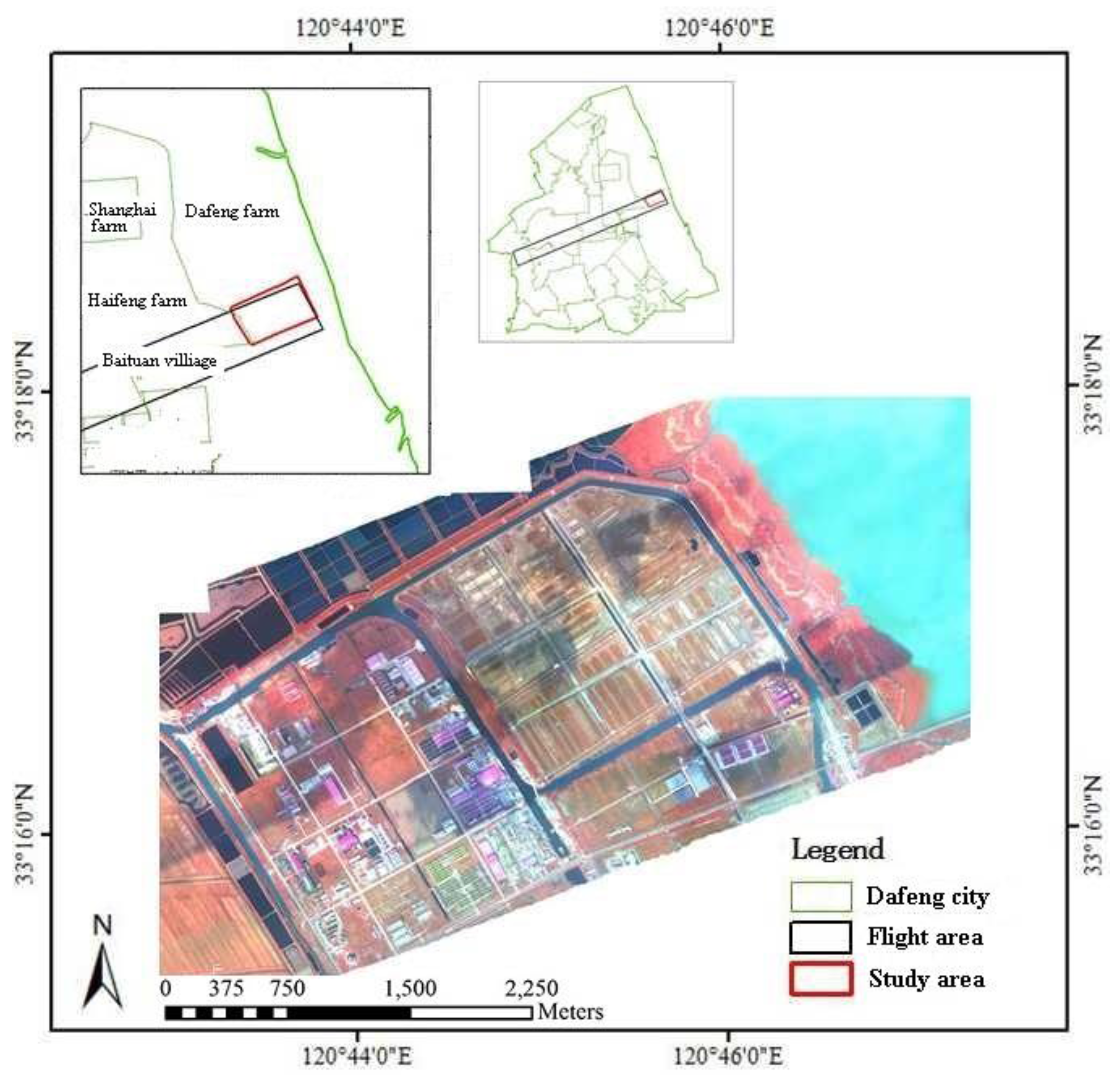
Figure 2.
Classification of wetland vegetation derived from LiDAR point cloud data. * High vegetation: high vegetation canopy height (>250 cm); medium vegetation: medium vegetation canopy height (30–250 cm); low vegetation: low vegetation canopy height (<30 cm).
Figure 2.
Classification of wetland vegetation derived from LiDAR point cloud data. * High vegetation: high vegetation canopy height (>250 cm); medium vegetation: medium vegetation canopy height (30–250 cm); low vegetation: low vegetation canopy height (<30 cm).
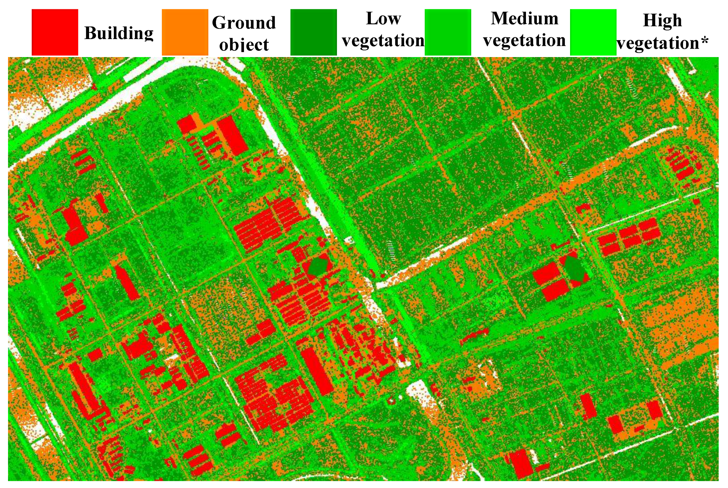
Figure 3.
DSM information derived from LiDAR point cloud data.

Figure 4.
Blue, green, red and near infrared bands and vegetation indexes derived from hyperspectral images ((a): blue band; (b): green band; (c): red band; (d): NIR; (e): RVI; (f): NDVI; (g): GNDVI; (h): DVI; (i): RDVI; (j): EVI; (k): TVI; (l): VARI; (m): ARVI; (n): GEMI).
Figure 4.
Blue, green, red and near infrared bands and vegetation indexes derived from hyperspectral images ((a): blue band; (b): green band; (c): red band; (d): NIR; (e): RVI; (f): NDVI; (g): GNDVI; (h): DVI; (i): RDVI; (j): EVI; (k): TVI; (l): VARI; (m): ARVI; (n): GEMI).
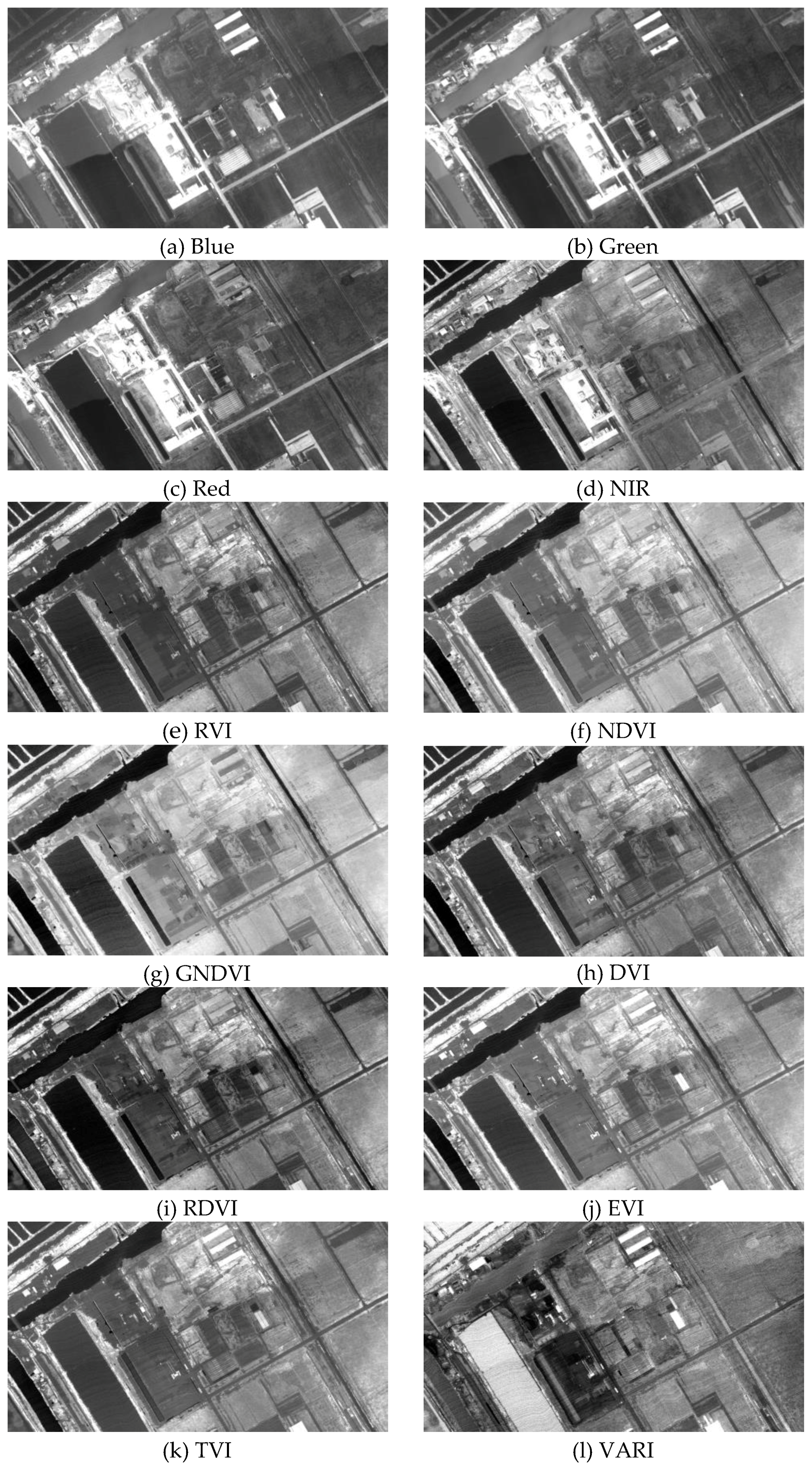
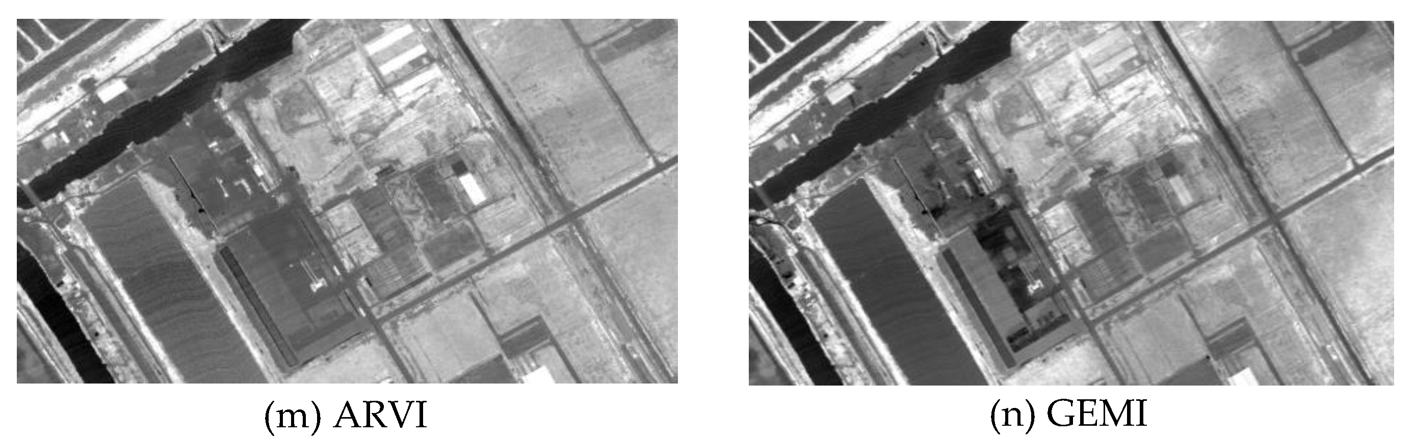
Figure 5.
Estimation error of S. alterniflora (a) and wetland vegetation (b).
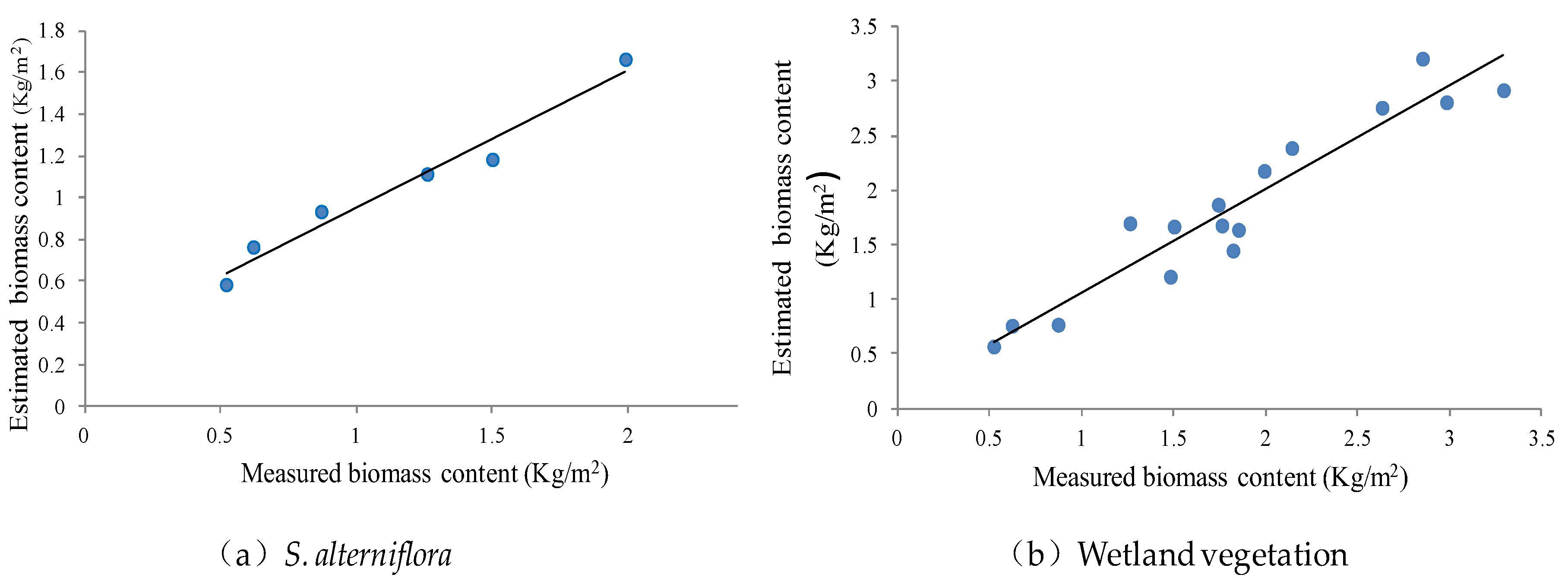
Figure 6.
Mapping biomass content of S. alterniflora using LiDAR data and hyperspectral images.


Table 1.
Correlation coefficients between wetland vegetation biomass and spectral parameter.
| VI | R452 | R534 | R694 | R865 | RVI | NDVI | GNDVI | DVI |
|---|---|---|---|---|---|---|---|---|
| Wetland | 0.515 ** | 0.639 ** | 0.087 | 0.546 ** | 0.007 | 0.006 | 0.071 | 0.488 ** |
| VI | RDVI | TVI | VARI | ARVI | GEMI | EVI | Height | |
| Wetland | 0.294 | 0.506 ** | 0.109 | 0.013 | 0.507 ** | 0.007 | 0.421 ** |
**: significantly correlated at significant level α = 0.05.
Table 2.
Multivariate linear estimation models of wetland vegetation biomass.
| Independent Variables Introduction | Multivariate Linear Estimation Models | R2 Value |
|---|---|---|
| Variables forced entry | Y = 35.684X1 − 3.531X2 + 7.582X3 − 0.078X4 + 0.18X5 − 1.061 | 0.650 |
| Variables forward entry | Y = 48.517X1 − 0.686 | 0.620 |
| Y = 35.411X1 + 0.124X5 − 1.228 | 0.704 | |
| Variable backward elimination | Y = 38.665X1 − 2.681X2 + 0.165X5 − 1.085 | 0.691 |
| Y = 35.446X1 − 3.559X2 + 7.582X3 + 0.179X5 − 1.083 | 0.672 | |
| Y = 35.684X1 − 3.531X2 + 7.582X3 − 0.078X4 + 0.18X5 − 1.061 | 0.650 | |
| Variable stepwise entry | Y = 35.411X1 + 0.124X5 − 1.228 | 0.704 |
| Y = 48.517X1 − 0.686 | 0.620 |
Note: X1 for R534, X2 for R865, X3 for R452, X4 for GEMI, and X5 for TVI.
Table 3.
Correlation coefficients between S. alterniflora biomass and spectral parameter.
| VI | R452 | R534 | R694 | R865 | RVI | NDVI | GNDVI | DVI |
|---|---|---|---|---|---|---|---|---|
| S. alterniflora | 0.090 | 0.135 | 0.024 | 0.196 | 0.520 ** | 0.635 ** | 0.241 | 0.238 |
| VI | RDVI | TVI | VARI | ARVI | GEMI | EVI | Height | |
| S. alterniflora | 0.320 | 0.254 | 0.599 ** | 0.631 ** | 0.284 | 0.288 | 0.817 ** |
**: significantly correlated at significant level α = 0.05.
Table 4.
Multivariate linear estimation models of S. alterniflora biomass.
| Independent Variable Introduction | Multivariate Linear Estimation Models | R2 Value |
|---|---|---|
| Variables forced entry | Y = 0.54X1 − 0.802X2 − 1.004X3 + 2.714X4 + 0.053X5 + 1.101 | 0.841 |
| Variables forward entry | Y = 0.514X1 + 1.11X4 + 0.388 | 0.902 |
| Y = 0.765X1 + 0.119 | 0.811 | |
| Variable backward elimination | Y = 0.514X1 + 1.11X4 + 0.388 | 0.902 |
| Y = 0.512X1 − 0.812X3 + 2.626X4 + 0.787 | 0.891 | |
| Y = 0.533X1 − 1.829X3 + 3.106X4 + 0.056X5 + 1.018 | 0.880 | |
| Y = 0.54X1 − 0.802X2 − 1.004X3 + 2.714X4 + 0.053X5 + 1.101 | 0.841 | |
| Variable stepwise entry | Y = 0.514X1 + 1.11X4 + 0.388 | 0.902 |
| Y = 0.765X1 + 0.119 | 0.811 |
Note: X1 for vegetation canopy height, X2 for NDVI, X3 for ARVI, X4 for VARI, and X5 for RVI.
© 2017 by the authors. Licensee MDPI, Basel, Switzerland. This article is an open access article distributed under the terms and conditions of the Creative Commons Attribution (CC BY) license (http://creativecommons.org/licenses/by/4.0/).
Share and Cite
MDPI and ACS Style
Wang, J.; Liu, Z.; Yu, H.; Li, F. Mapping Spartina alterniflora Biomass Using LiDAR and Hyperspectral Data. Remote Sens. 2017, 9, 589. https://doi.org/10.3390/rs9060589
AMA Style
Wang J, Liu Z, Yu H, Li F. Mapping Spartina alterniflora Biomass Using LiDAR and Hyperspectral Data. Remote Sensing. 2017; 9(6):589. https://doi.org/10.3390/rs9060589
Chicago/Turabian StyleWang, Jing, Zhengjun Liu, Haiying Yu, and Fangfang Li. 2017. "Mapping Spartina alterniflora Biomass Using LiDAR and Hyperspectral Data" Remote Sensing 9, no. 6: 589. https://doi.org/10.3390/rs9060589
Note that from the first issue of 2016, this journal uses article numbers instead of page numbers. See further details here.