
Mapping of Urban Surface Water Bodies from Sentinel-2 MSI Imagery at 10 m Resolution via NDWI-Based Image Sharpening

1
ICube Laboratory, University of Strasbourg, 67081 Strasbourg, France
2
School of Earth & Space Sciences, Peking University, Beijing 100080, China
3
Depart of Computing Science, University of Alberta, Edmonton, T6G 2R3, Canada
4
School of Software, Yunnan University, Kunming 650091, China
5
School of Software & Microelectronucs, Peking University, Beijing 100080, China
*
Author to whom correspondence should be addressed.
Remote Sens. 2017, 9(6), 596; https://doi.org/10.3390/rs9060596
Submission received: 22 March 2017
/
Revised: 14 May 2017
/
Accepted: 10 June 2017
/
Published: 12 June 2017
Abstract
:This study conducts an exploratory evaluation of the performance of the newly available Sentinel-2A Multispectral Instrument (MSI) imagery for mapping water bodies using the image sharpening approach. Sentinel-2 MSI provides spectral bands with different resolutions, including RGB and Near-Infra-Red (NIR) bands in 10 m and Short-Wavelength InfraRed (SWIR) bands in 20 m, which are closely related to surface water information. It is necessary to define a pan-like band for the Sentinel-2 image sharpening process because of the replacement of the panchromatic band by four high-resolution multi-spectral bands (10 m). This study, which aimed at urban surface water extraction, utilised the Normalised Difference Water Index (NDWI) at 10 m resolution as a high-resolution image to sharpen the 20 m SWIR bands. Then, object-level Modified NDWI (MNDWI) mapping and minimum valley bottom adjustment threshold were applied to extract water maps. The proposed method was compared with the conventional most related band- (between the visible spectrum/NIR and SWIR bands) based and principal component analysis first component-based sharpening. Results show that the proposed NDWI-based MNDWI image exhibits higher separability and is more effective for both classification-level and boundary-level final water maps than traditional approaches.
1. Introduction
Urban surface water bodies, which significantly influence public health and the living environment, are important parameters in urban planning, regional climate, and the heat island effect. Rapid urbanisation increasingly leads to the damage and decline of water bodies, which makes the dynamic monitoring of the boundary of water bodies necessary. Numerous techniques have been applied to characterise and quantify water bodies using either ground measurements of field surveys or remotely sensed data. Remote sensing provides repetitive mapping in time- and cost-saving modes. Various remote sensing data have been utilised in water surface mapping, including Synthetic Aperture Radar (SAR) satellites [1,2], LiDAR data [3], and various spatial resolution optical satellite images ranging from low-resolution [4,5] to very high-resolution imagery [6,7].
Images from moderate-resolution optical satellites, such as Landsat, Advanced Spaceborne Thermal Emission and Reflection Radiometer (ASTER) and Satellite Pour l’Observation de la Terre (SPOT), exhibit vivid spectral information (typically Near InfraRed (NIR) and Short-Wavelength InfraRed (SWIR) bands for water information), large area, and high-frequency coverage. These images have been the most utilised data sources for providing timely and accurate approaches to monitor surface water bodies. At present, numerous methods have been developed to delineate water bodies in moderate-resolution satellite imagery. These methods can be categorised into three types according to mapping level: (i) pixel-based statistical pattern recognition analysis, including supervised [8,9] and unsupervised [10] classification approaches; (ii) object-based image analysis techniques with different parameters, such as spectral features, texture, shape complexity and relationship [11]; and (iii) sub-pixel mapping with spectral mixture analysis [12]. Regardless of the method used, water indices are generally calculated to enhance the separation between water bodies and other objects. Zhou et al. compared the performance of different water indices in Landsat 7 ETM+, Landsat 8 Operational Land Imager (OLI) and Sentinel-2 MSI [13]. Fisher et al. proposed a new Landsat Thematic Mapper (TM)/ Enhanced Thematic Mapper Plus (ETM+)/OLI water index based on surface reflectance and compared different water indices, which revealed different errors for different water and non-water types [14]. Yao et al. proposed a new water index based on pixel-wise coefficient calculation and utilised a support vector machine to train related parameters with ZiYuan-3 multispectral images [15]; Yang et al. collected water and vegetation, and built-up indices to construct a unique feature matrix for each pixel and then applied deep learning to realise water mapping in Landsat imagery [16]; and Ko et al. constructed boosted random forest classifiers by combining Top-Of-the-Atmosphere (TOA) reflectance and the values of water indices [17]. To delineate the free water surface boundary, excluding the moisture/muddy lake water, Singh et al. combined tasselled cap transformation, Hue Saturation Value (HSV) colour transformation, high-pass filtering, vector analysis, and object segmentation on the basis of the water index calculation. [18]. Xie et al. first applied a water index for the automatic extraction of mixed land–water pixels, and then the pure water pixels generated from this process were exported as the final result. Subsequently, spectral mixture analysis was applied to the mixed land–water pixels to estimate water abundance [12]. Zhou et al. combined object-level multiscale extractions and sub-pixel spectral mixture analysis techniques in adaptive local regions, and then the images of the water indices were calculated to select water sample pixels [11].
The combination of the images of water indices with other object extraction techniques has resulted in progress in water body mapping, particularly of extensive coastal areas, large lakes, dramatic rivers, and lacustrine or potamic water bodies in rural areas [19]. Water bodies in urban areas [12] are frequently small and surrounded by complex built-up areas, vegetation, and their shadows. The fragmented surface constituents result in a considerable amount of mixed pixels, category confusion between water and complex features, and high spectral variance of water bodies. A high resolution can reduce the number of mixed pixels and provide a distinguishable boundary, which can improve the accuracy of urban surface water boundary definition.
The Sentinel-2 mission, organised by the Global Monitoring for Environment and Security (GMES), acquires multispectral, high-resolution optical observations over global terrestrial surfaces with a high revisit frequency of approximately 5 days using a bi-satellite system. Such a system is important for dynamic land cover mapping and updating. [20] Sentinel-2 carries a MultiSpectral Instrument (MSI) with 13 spectral bands spanning from the VIsible Spectrum (VIS) and NIR to SWIR at different spatial resolutions on the ground ranging from 10 m to 60 m with a 290 km field of view. With high time resolution and spectral resolution, Sentinel-2 exhibits the advantage of intensively and continuously monitoring the surface of the Earth. Sentinel-2 MSI imagery includes 20 m resolution SWIR bands and 10 m resolution green and NIR bands, thereby making water mapping based on water indices at 10 m resolution possible.
Image pan-sharpening typically fuses high spatial resolution panchromatic data with low-resolution multispectral imagery. Such fusion creates a product with the spectral characteristics of MSI and a spatial resolution that approaches that of a panchromatic image [21]. Panchromatic sharpening is an important image fusion technique for numerous moderate remote sensing applications, particularly classification, segmentation, and object detection. This technique is commonly used to compensate for the spectral/spatial compromise in satellite imaging, typically for imagery equipment with high-resolution pan band and low-resolution multispectral bands, such as SPOT and the Landsat 8 OLI.
Sentinel-2 MSI no longer provides panchromatic band imagery and instead enhanced its VIS and NIR band images to a relatively high spatial resolution (10 m). The problem arises from the use of the pan-like high resolution band to sharpen other multi-spectral bands (20 m and 60 m). Normally, certain bands that are most related to SWIR [22] are typically utilised as high-resolution bands to provide spatial information.
The main contribution in this paper is to construct a pan-like band with the Normalised Difference Water Index (NDWI) spectral index (10 m) to downscale other multi-spectral bands. This pan-like band is expected to enhance the difference between water bodies and other objects during the image sharpening process. Specifically, the SWIR bands are improved to higher spatial resolution in 10 m and the corresponding Modified NDWI (MNDWI) [23] is calculated for further urban surface water extraction mapping.
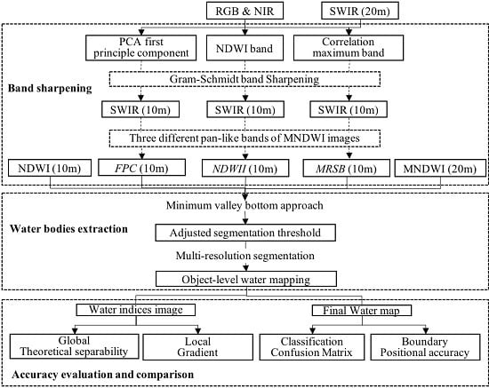
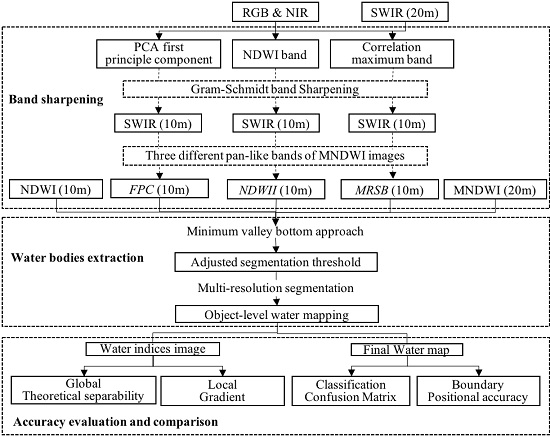
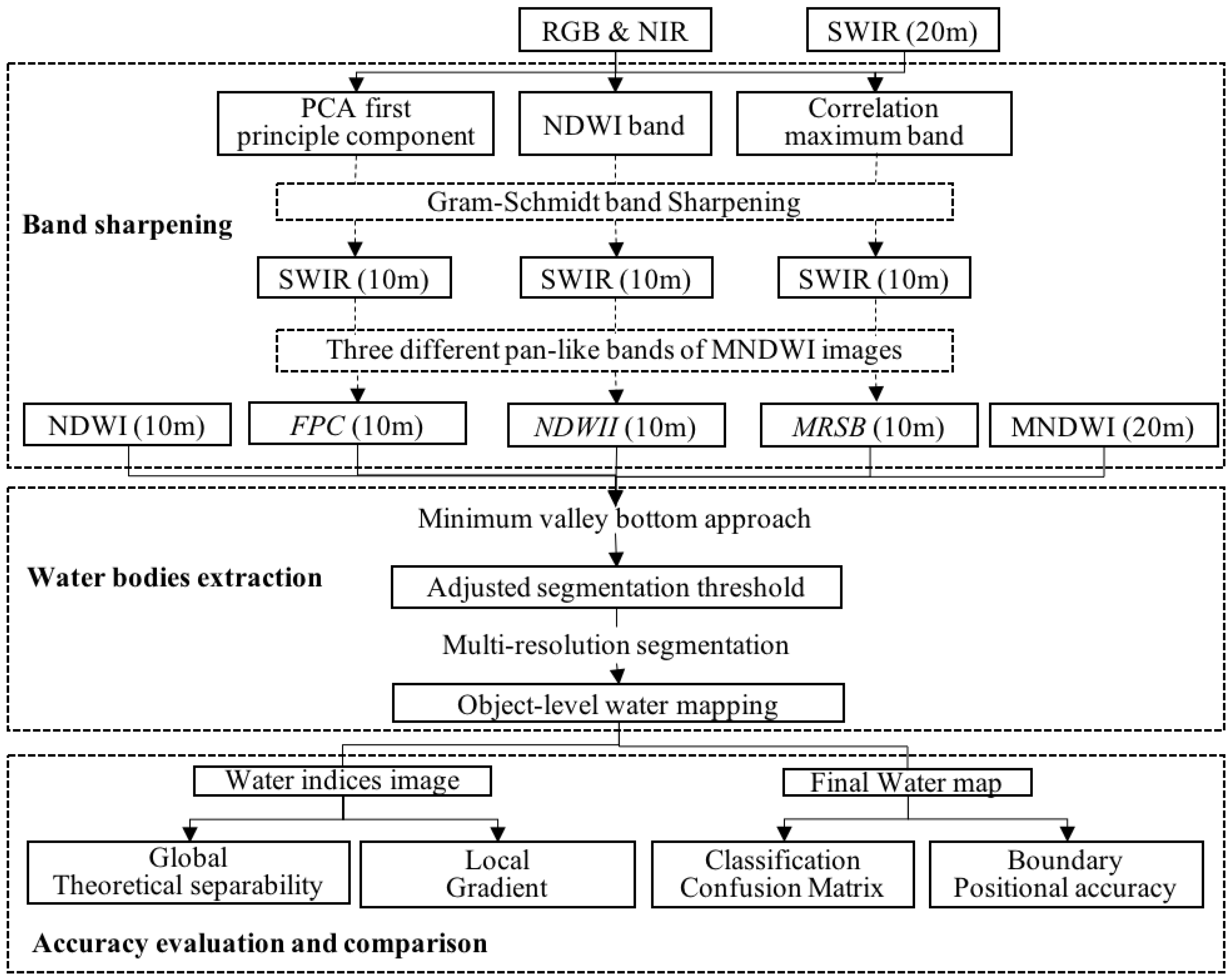
The proposed NDWI Image- (NDWII) based pan-like sharpening method (Figure 1), which combines the minimum valley bottom automatic threshold approach and object-level water mapping, is compared with the conventional Most Related Single Band (MRSB) method [22] and the dimension-reducing Principal Component Analysis (PCA) and First Principal Component (FPC) techniques. Lastly, the method is evaluated in two study areas using a classification confusion matrix and boundary position accuracy in the final water maps and water separability in the images of water indices with three different inputting high-resolution pan-like bands.
2. Materials and Methods
2.1. Study Areas and Materials
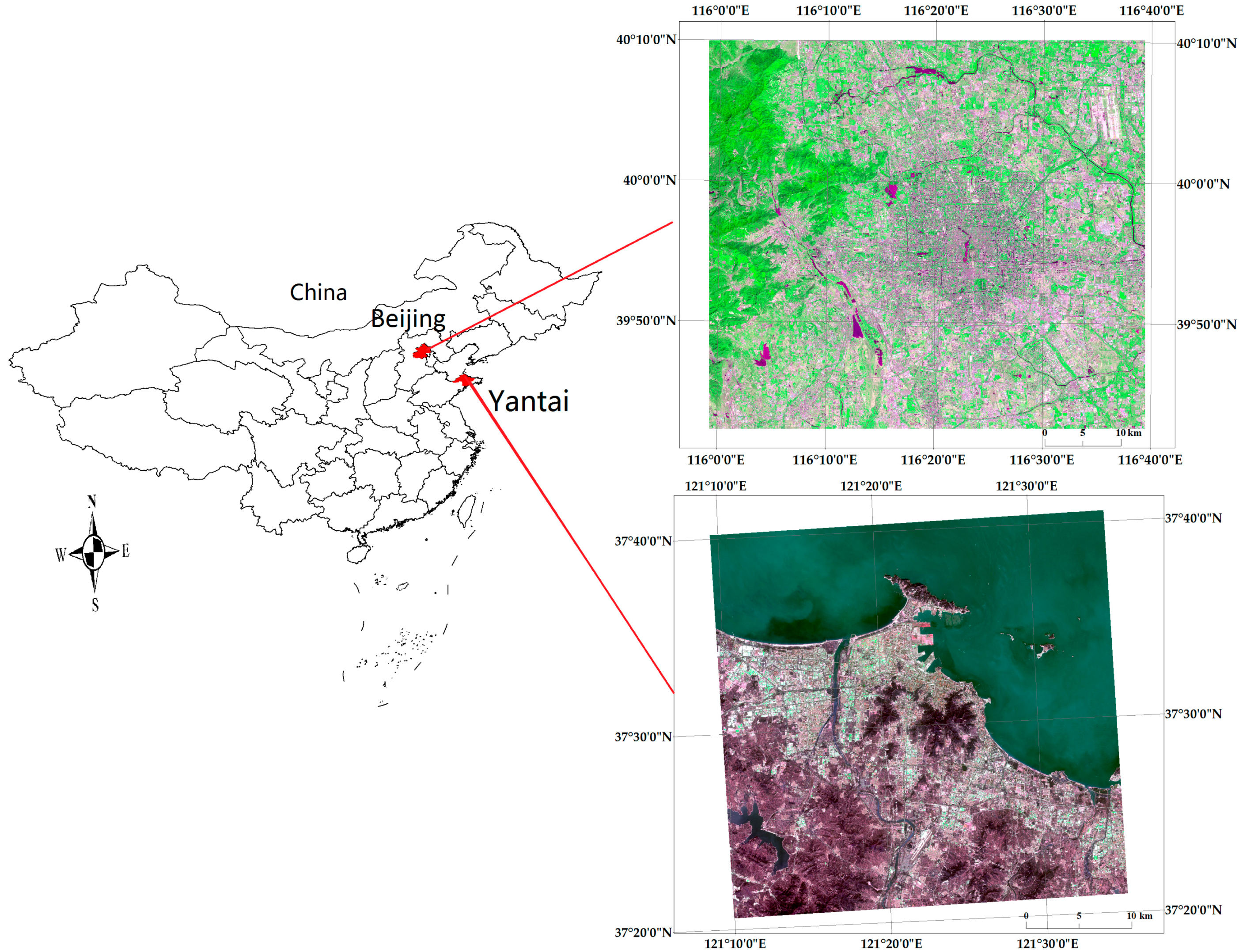
The study areas (Figure 2) comprised two separate cities in China, namely, Beijing, which is located inland, and Yantai, which is located in a coastal area. The Sentinel-2A satellite images used in this study were collected on 3 May 2016 (Beijing) and 10 October 2016 (Yantai) under clear weather conditions. The data contained 13 spectral bands with different spatial resolutions. However, only 3 VIS bands and 1 NIR band with a spatial resolution of 10 m, and 2 SWIR bands with a resolution of 20 m, which were closely related to water information, were utilised in this study. The adopted Sentinel-2 level 1C dataset was the standard product of TOA reflectance, which was more suitable for calculating water indices compared with the raw digital number value. Thus, additional pre-processing [24] was not required, and the water indices for the MSI images could be directly calculated. We clipped a 57 × 51 km area (Beijing) and a 37 × 36 km area (Yantai) of 5737 × 5107 pixels and 3736 × 3630 pixels, respectively, from the original multispectral imagery for mapping water bodies (Figure 2). The first study area encompassed a downtown district and surrounding suburban areas, in which water bodies include a few sparsely distributed ponds, rivers, and park lakes. These water bodies are relatively small and surrounded by built-up areas and vegetation. In particular, the extensive occurrence of high-rise buildings and street trees formed an abundance of shadowed areas. The second study area is located along the north coast of the Shandong Peninsula and south of the Bohai Sea. Its water bodies include rivers, lakes, and recognisable coast. ‘True’ water bodies are manually digitised by a visual interpretation process of the Sentinel-2 image with reference to Google Earth.
2.2. Method
2.2.1. Water Indices
McFeeters [25] proposed the most well-known NDWI (Equation (1)) using green and NIR bands to maximise the reflectance of a water body in the green band while minimising that in the NIR band. NDWI can effectively enhance the water information in most cases; however, it is sensitive to built-up land and frequently results in overestimated water bodies [22].
Xu [24] proposed MNDWI (Equation (2)) by replacing the NIR band used in NDWI with the SWIR band to overcome the inseparability of built-up areas. In general, water bodies have larger positive values in MNDWI compared with NDWI because they generally absorb more SWIR light than NIR light. Soil, vegetation, and built-up classes have smaller negative values because they reflect more SWIR light than green light. MNDWI, which has demonstrated its superiority in many applications related to water bodies, including urban surface water extraction, is extensively used once a SWIR band is available.
2.2.2. Band Sharpening Methods
The SWIR bands in Sentinel-2 MSI images are at 20 m resolution and can be improved to 10 m by utilising the band sharpening algorithm. The sharpened band is combined with multispectral characteristics and high spatial resolution. Multispectral information is useful for extracting and identifying water bodies, which refers to the calculation of water indices in this study. The increased spatial resolution can help improve boundary extraction accuracy and reduce the category confusion phenomenon, which are particularly important in urban scene.
Imagery from traditional moderate-resolution satellites, such as the Landsat and SPOT series, provides high-resolution panchromatic bands to specifically sharpen low-resolution multispectral images. Through enhanced data storage and transmission, the Sentinel-2 MSI directly acquires high-resolution images in VIS and NIR bands to replace the unique panchromatic approach, thereby providing multiple choices for inputting high-resolution pan-like bands as follows.
(i) MRSB. The general concept regarding image fusion is to reserve the original multispectral information in the sharpening process; therefore, recent works [22,26] tend to choose the band most related to the SWIR band. In general, the band with the highest correlation coefficient (Equation (3)) with the SWIR band is selected as the most suitable pan-like band. In the current study, the NIR band was chosen as the pan-like band in both the Yantai study area and the Beijing study area (SWIR 2 band) (Table 1); the Green band is chosen as the pan-like band for the SWIR 1 band in the Beijing study area.
where N is the number of pixels in the SWIR band at 20 m resolution, VN is the VIS/NIR band at the spatial resolution of 20 m that was generated by upscaling the original 10 m images and and are mean values of SWIR and VIS/NIR, respectively.
(ii) PCA FPC. The typical PCA FPC can support the demand with most of the information to compress the four bands into a single pan-like band. PCA is extensively used in remote sensing multispectral image analysis. Multispectral bands have various degrees of correlation, which results in data redundancy. A mutually orthogonal spectral space is generated through the linear transformation of the four-band multispectral image, and its FPC includes the most information. Thus, one pan-like band is obtained from the main information among the entire VIS/NIR bands.
(iii) NDWI Image (NDWII). Although water bodies are difficult to distinguish from a complex urban land surface, NDWII enhances the information of water bodies, and particularly highlights boundary information. In this study, the NDWI at 10 m resolution is used as a high-resolution band to sharpen the SWIR bands with enhanced water information.
Several well-known pan-sharping algorithms, such as PCA, HSV, and Gram–Schmidt (GS), are available. Among these algorithms, GS exhibits the highest fidelity, which maintains the consistency of image spectral characteristics before and after pan-sharpening [27]. The spectral characteristics of low spatial resolution multispectral data are preserved in the high spatial resolution sharpened multispectral data. Thus, the GS sharpening approach [28] is adopted in this study to reserve the spectral information for calculating water indices and dealing with water bodies with high-resolution NDWI bands.
2.2.3. Threshold Segmentation
An automatic framework that integrates pixel-level threshold adjustment (minimum valley bottom of the grey histogram) and object-oriented multi-scale segmentation (eCognition software [29]) is proposed to realize water mapping.
After enhancing the difference between water bodies and other objects, the pixels of the water bodies can be extracted through binary segmentation using a suitable threshold value. Threshold selection is a key step in extracting water pixels from water index images. The use of an empirically selected threshold (normally zero) can overestimate or underestimate water area because threshold values vary among regions depending on different image characteristics [30,31].
Various threshold adjustment methods have been proposed by utilising different information, including histogram shape, measurement space clustering, entropy, attribute similarity, spatial correlation, and local grey-level surface [32]. The imaging of water indices exhibits a polarisation trend wherein the pixel values of water bodies return positively large values, whereas those of other objects tend to be theoretically negative. Thus, the image histogram is characterised by a smoothed, two-peaked representation of the distribution of foreground and background pixels. Otsu’s method [33], which is based on histogram shape, has been conventionally used in surface water extraction. However, this method yields unstable results when a small area of water bodies and large built-up areas exist.
In this study, we analyse the two-peak distribution in the grey histogram, compare several threshold adjustment methods (Figure 3), and draw the conclusion to set the minimum value in the valley bottom between the double peaks as the threshold.
In general, threshold segmentation can extract water pixels and obtain water mapping. In urban areas, the spectral similarity between water and other dark objects results in a dramatic ‘pepper phenomenon’, which comprises sparse pixels. Object-level multi-scale segmentation is conducted by the eCognition software to build homogeneous blocks, and the spectral mean value of each element is calculated. The segmented blocks are labelled as water if the spectral mean value is larger than the obtained threshold based on the histogram calculation. Such integration can eliminate the noise of small building shadows to a certain extent. However, dealing with the spectral similarity between water bodies and other built-up areas and vegetable shadows remains difficult.
2.3. Accuracy Evaluation
2.3.1. Water Separability
A water index is designed to enhance the contrast between water and non-water pixels. The combination of optimal bands should be determined to accurately and robustly discriminate water from other land cover types [15]. The threshold segmentation approach based on water indices depends on the spectral difference between water and non-water areas. In general, a distinct separation is expected between the double peaks in the grey histogram, which represent water and non-water areas, thereby confirming two normal distributions: and . Therefore, to extract water bodies, theoretical separability is estimated by calculating pixel value distribution based on the reference mapping of water and non-water areas (Figure 4). The use of two degrees of confidence levels (95% and 90%) is justified, which indicates that 95% and 90% of the intervals obtained from such classification will contain the true category. One-side lower/upper confidence limits are separately performed for the water and non-water normal distributions, which can be calculated as Equation (4). In particular, 1.96 and 2.235 are respectively the 0.975 and 0.95 one-side quantiles of the normal distribution.
Then, two different relationships between the two histograms can be obtained: separation, if the lower limit > the upper limit, which means the water and non-water bodies are well distinguishable, and mixture, if the lower limit < the upper limit, which means that some water and non-water pixels cannot be classified. The separation rate and mixture rate can be calculated as and . Evidently, the adopted minimum bottom valley threshold adjustment approach is closely related to the separation rate and mixture rate. The higher the separation rate or the lower the mixture rate, the easier the image can be segmented.
This factor is used to evaluate to what extent the water index image could enhance the difference between the water and non-water pixels. The pixel value statistics regarding separability are based on the correct identification of water and non-water pixels without noise. Pixels with false classification are excluded from the histograms. Therefore, such statistics display the theoretical mixture and separation of water and non-water pixels in the water index image. Classification accuracy also depends on the real optimal threshold value.
2.3.2. Water Mapping
The classical confusion matrix is adopted to evaluate extraction class accuracy and the effectiveness of the proposed NDWI-based band sharpening approach. In addition, a special section is provided to discuss the boundary position accuracy of the proposed boundary index.
Unit rates (Equation (5)) based on the confusion matrix are utilised to evaluate the final water maps produced using different water indices, including Producer’s Accuracy (PA), User’s Accuracy (UA), Overall Accuracy (OA), and Kappa coefficient (Kappa):
, T is the total number of the pixels in the experimental Sentinel-2 image, and are the categorized pixels by comparing the extracted water pixels with the reference map:
- TP: true positives, i.e., the number of correct extraction;
- FN: false negatives, i.e., the number of the water pixels not detected;
- FP: false positives, i.e., the number of incorrect extraction;
- TN: true negatives, i.e., the number of non-water bodies’ pixels that were correctly rejected.
The boundary is important for water bodies, particularly for coastlines, shorelines, and riparian lines. The classification accuracy of water bodies cannot reflect boundary conditions. We further evaluate the performance of boundary extraction using the Boundary Index (BI), which is the ratio between the extracted boundary and the reference boundary (Figure 5). The extracted boundary is calculated through the intersection judgment with the buffering area of the reference boundary. Thus, BI is applied to evaluate the accurate boundary recognition of lake, coastal, and river bank lines.
3. Experimental Results and Evaluation
3.1. Images of Water Indices and Adjusted Threshold
When the typical evaluation methods for spectral and spatial qualities, such as the correlation coefficient and the root mean square error [6] of the generated sharpened images, are used, the three different input high-resolution bands present similar results close to 99%. The subsequent MNDWI images and pixel-wise threshold segmentation images at 10 m resolution from the sub-area of the Beijing Sentinel-2 MSI image are shown in Figure 3.
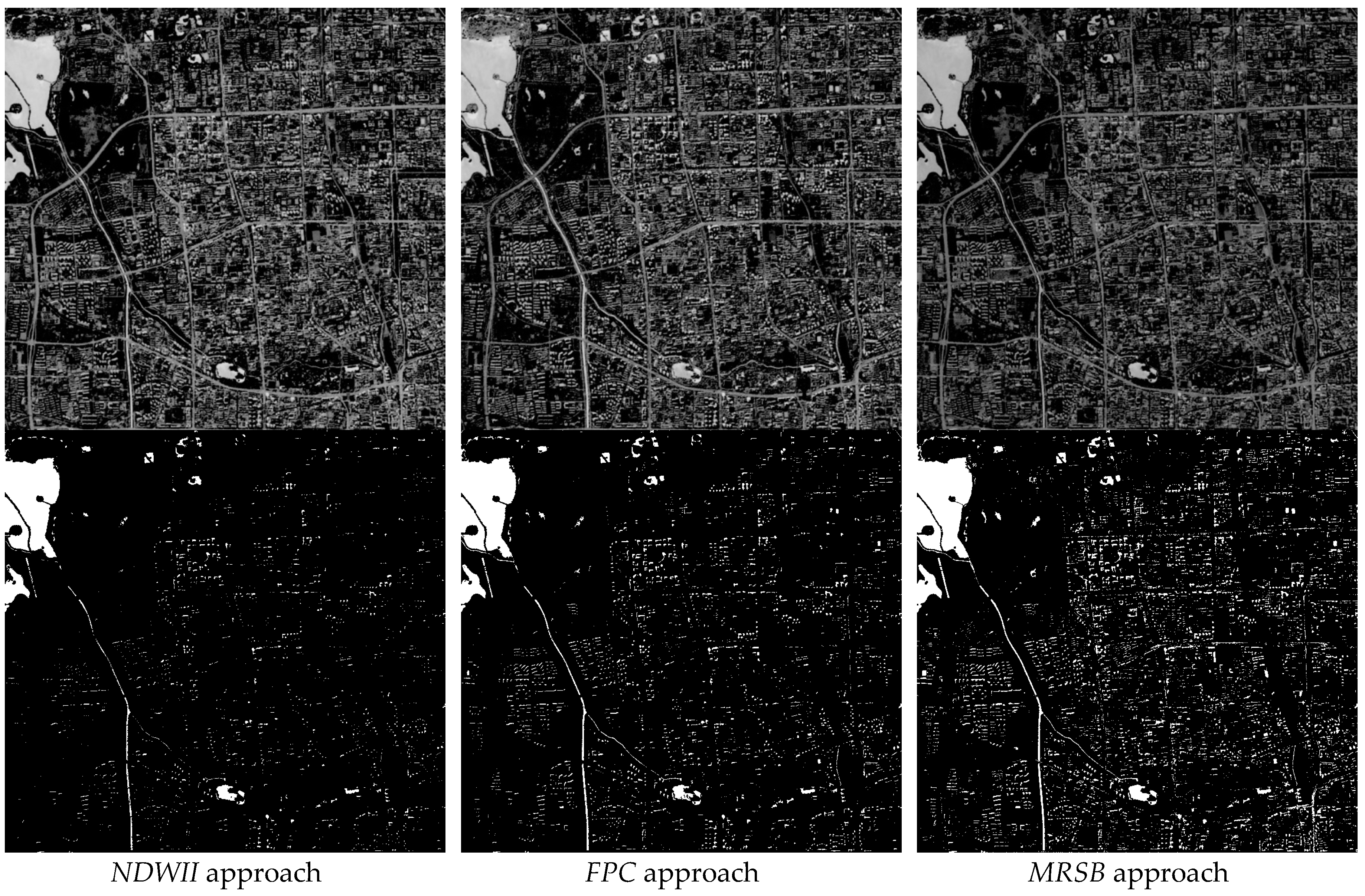
The three MNDWI images and pixel-wise water extraction obtained from the three pan-like bands, namely, the proposed NDWII, PCA FPC, and conventional MRSB, are comparatively shown in Figure 6. The sparse shadow blocks in the pixel-level can be eliminated to a certain degree in the object-level water mapping, thereby showing the spectral difference between the water and non-water areas under different pan-like bands. A close visual inspection of the images will present their main difference, which is the relative restraint of the dark shadowed areas in the NDWI-based high-resolution band compared with the other two bands.
3.1.1. Spectral Value Category Histogram at the Global Level
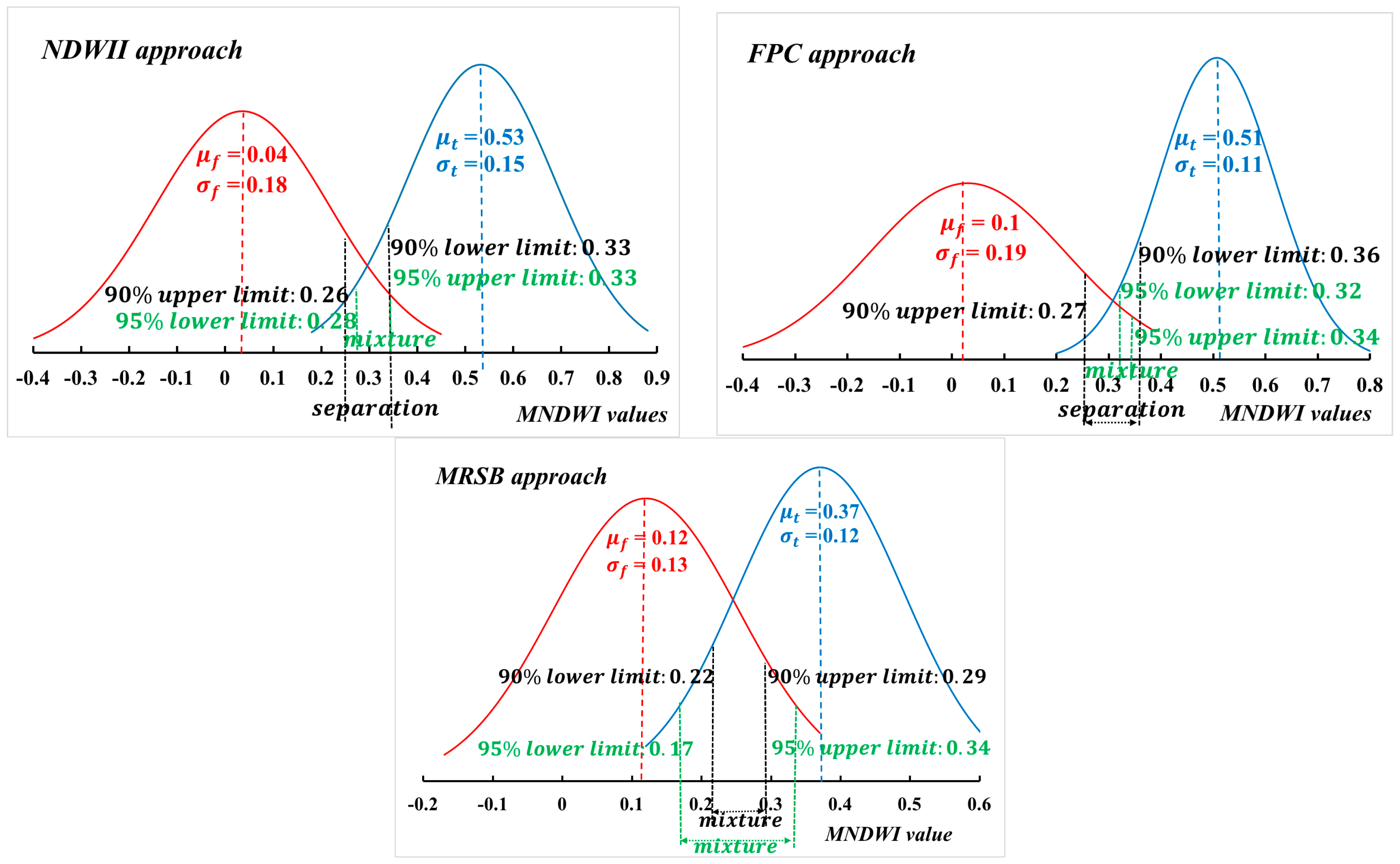
Figure 7 shows the corresponding theoretical separation in different MNDWI images (the first row of Figure 6). Under the 95% confidence interval, NDWII, FPC, and MRSB return mixture rates of 0.11, 0.16, and 0.66, respectively. Under the 90% confidence interval, NDWII and FPC obtain separation rates of 0.14 and 0.09, respectively, whereas MRSB still returns a mixture rate of 0.29. If the theoretical minimum valley bottom values in the histograms are selected, then NDWII and FPC can efficiently extract water bodies with thresholds of 0.3 and 0.32, respectively, which lie in the separation areas under the 90% confidence interval. Meanwhile, MRSB exhibits extreme misclassification because of spectral mixture. This result shows a higher possibility of water extraction using NDWII or FPC then using MRSB. NDWII or FPC may obtain more accurate classification results with less error delineation than MRSB.
3.1.2. Local-Level Evaluation
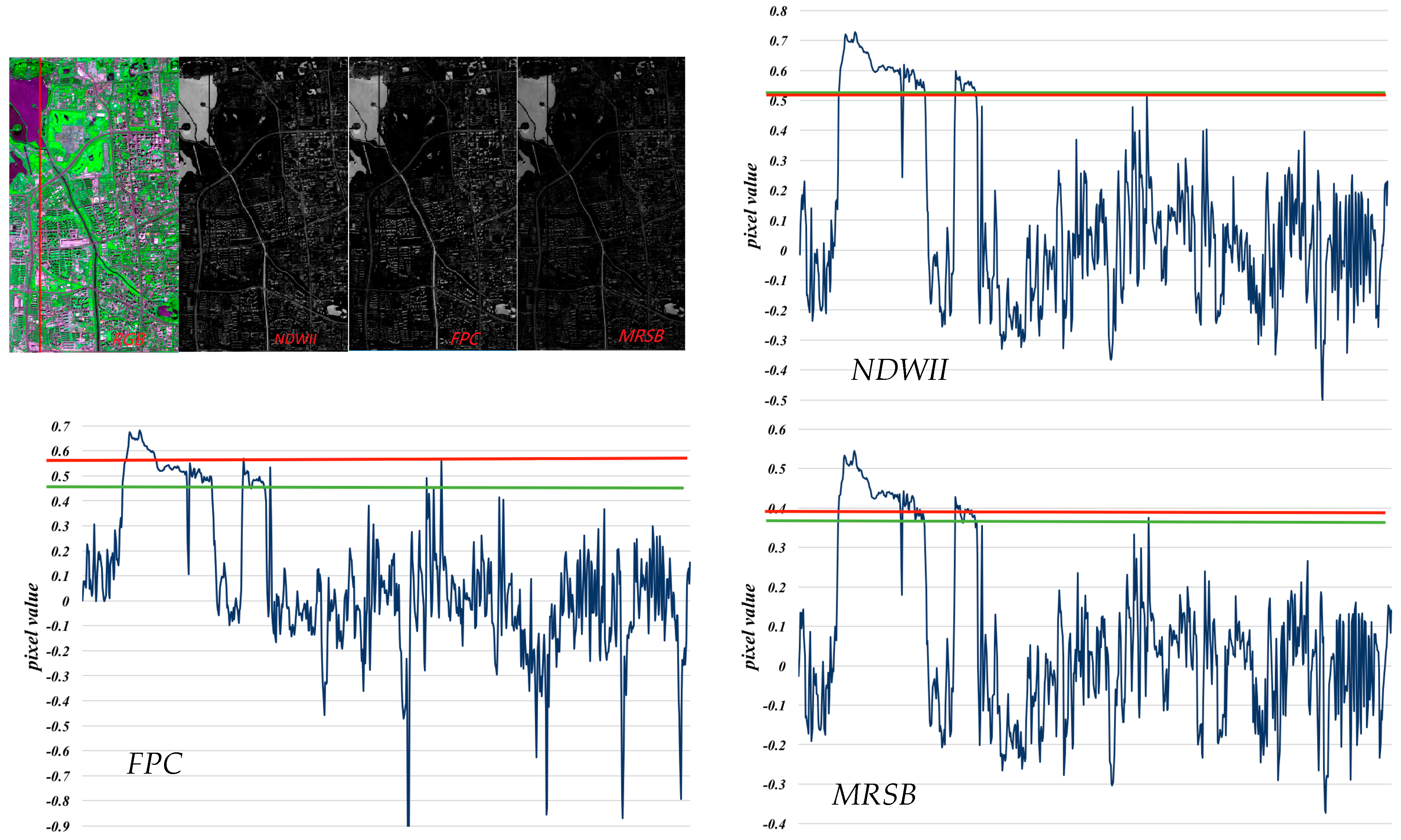
To clearly display the separation between the water and non-water areas, a linear cover line is selected to pass by the water areas and the typical mixture road. The change in the water index value is presented as a curve in Figure 8. The main difficulty in the displayed sub-area is the similar spectral values of the dark road (the yellow box in the image and the histograms) and the lake bodies. Evidently, the road and the water areas have similar spectral values, which are difficult to distinguish via spectral-based classification. For the NDWII-based result, the water area can be correctly identified under manual threshold conditions. For the MRSB- and PCA- FPC-based results, the complete water extraction (green line) and accurate extraction (red line) are difficult to consider simultaneously. The NDWII-based approach can realise accurate segmentation once the exact threshold is obtained.
3.2. Mapping of Water Bodies
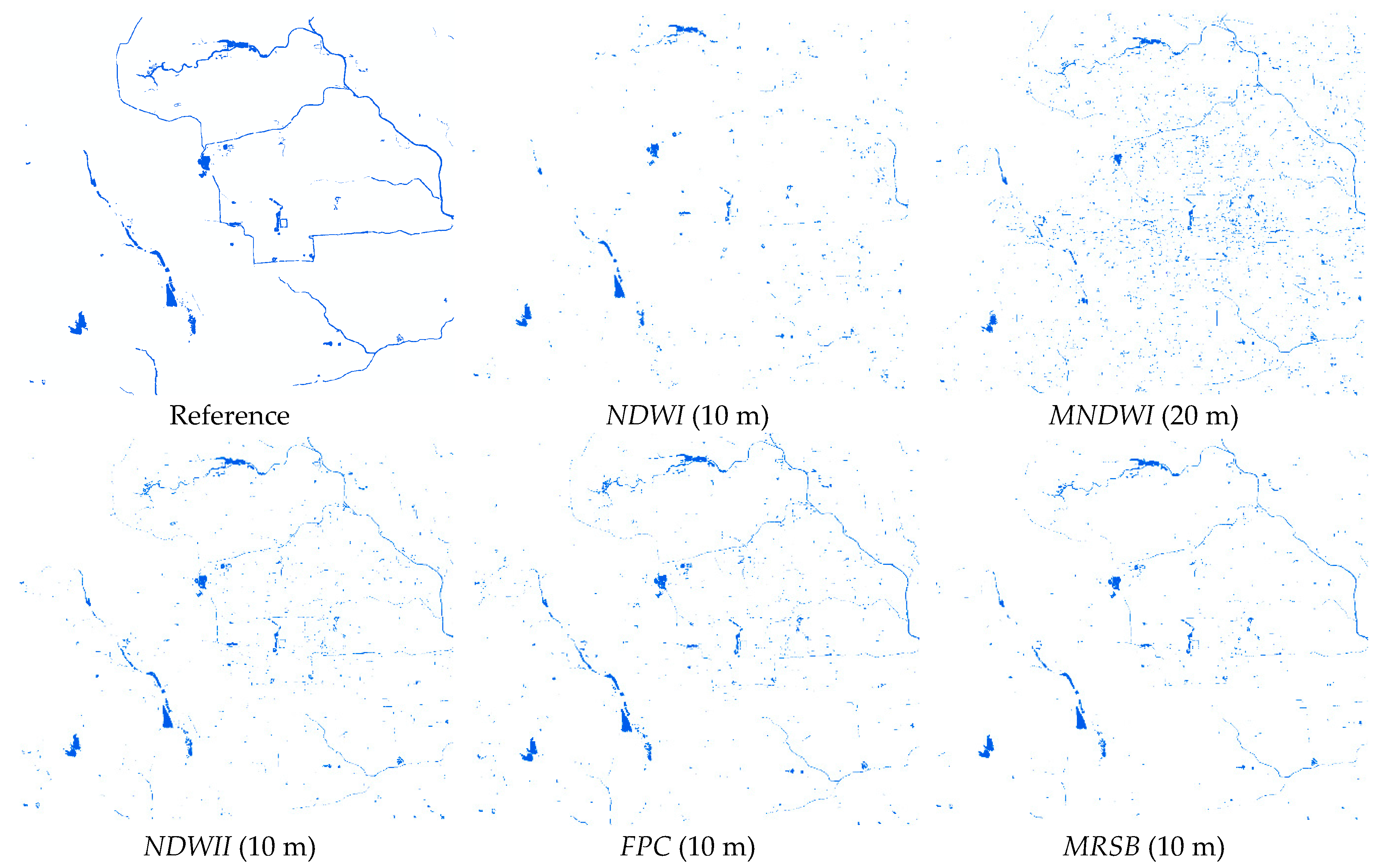
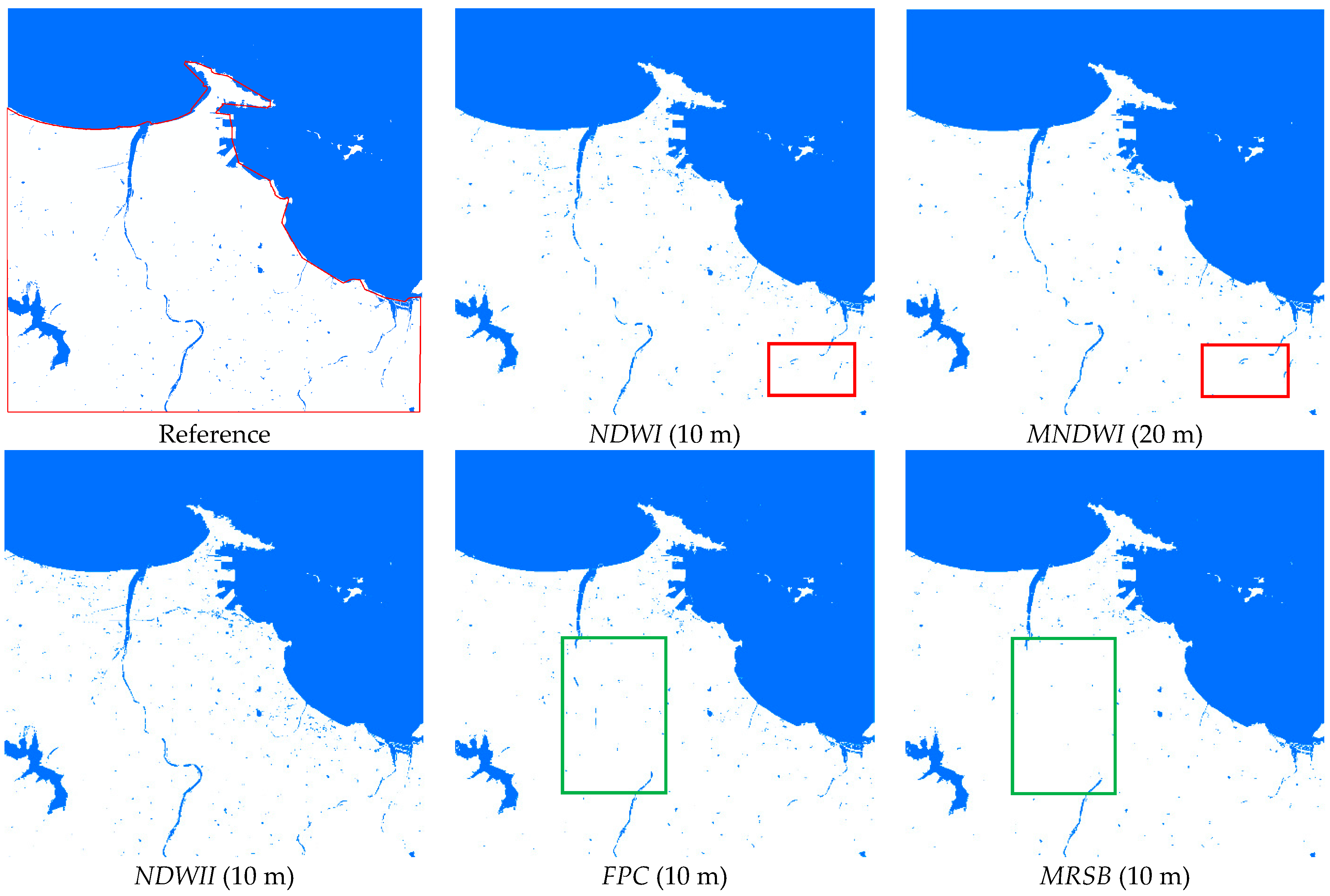
The three methods for sharpening the MNDWI are compared with the original NDWI (at 10 m resolution) and MNDWI (at 20 m resolution) to determine the accuracy of water mapping with different high-resolution input pan-like bands. All five mapping images of the water indices in the Beijing and Yantai study areas are comparatively presented in Figure 9 and Figure 10, respectively.
In general, all the water indices can extract the typical water areas with the adjusted threshold values. For the Beijing District, the results from the sharpened MNDWI are visually cleaner and more robust compared with the original NDWI (10 m) and MNDWI (20 m). The three sharpening-based approaches, namely NDWII, FPC, and MRSB, exhibit reliable results that have detected most water bodies. MNDWI (20 m) loses several typical water bodies (in the yellow box) and consists of extreme sparse noise, thereby showing the importance of spatial resolution in reducing ambiguity. Meanwhile, NDWI fails to detect most of the rivers in the downtown areas, which agrees with the fact that NDWI is not feasible for extracting water bodies surrounded by built-up areas on an urban surface. For the Yantai District, the NDWII approach detects the main body of the rivers. The NDWI (10 m) and MNDWI (20 m) approaches are lacking for the small river (in the red box), whereas the FPC and MRSB approaches fail to extract a large portion of the river (in the green box). The misidentified water pixels are found in residential areas, particularly in shadows and dark roads. Beijing consists of large areas of high buildings and their shadows; hence, its water mapping result is not as clean as that of Yantai. In conclusion, band sharpening can help in water extraction and eliminate errors to a certain degree, particularly in the NDWII-based image sharpening approach, which yields the most robust results in both study areas.
3.2.1. Classification-Level Evaluation
Table 2 summarises the extraction accuracy and Kappa statistics of water mapping with NDWI, MNDWI, and different sharpened MNDWI images. For the study area in Yantai, the water classification accuracy is nearly the same under different water indices, in which the Kappa coefficient is between 0.839 and 0.878, and the overall accuracy is approximately 99%. However, for the study area in Beijing with numerous built-up areas surrounding small water bodies, band sharpening is necessary for water extraction., With a Kappa coefficient of approximately 0.9, the sharpened MNDWI yields more accurate results than NDWI (with a Kappa coefficient of 0.645) and low-resolution MNDWI (with a Kappa coefficient of 0.799), which is in accordance with the theoretical results. Nevertheless, McFeeters’ NDWI is limited by its inability to suppress noise from the land cover features of built-up areas, the low spatial resolution result in an apparent category mixture, and the large width of a recognisable river.
With regard to the three pan-like bands, NDWII and FPC have relatively high PA, which indicates a low omission error; that is, the detection of water is feasible. Similar to the main river in Yantai, only NDWII succeeds in extracting the main body. However, MRSB has a high UA, which indicates a low commission error. This result agrees with the visual analysis, in which clean maps with sparse noise were obtained using MRSB in both Beijing and Yantai. Both PA and UA are close to the threshold. A low threshold will increase PA, whereas a high threshold will increase UA. Nevertheless, the threshold is automatically defined using the same rule, and NDWII and FPC exhibit better overall accuracy and Kappa coefficients than MRSB.
3.2.2. Boundary Evaluation of Water Bodies
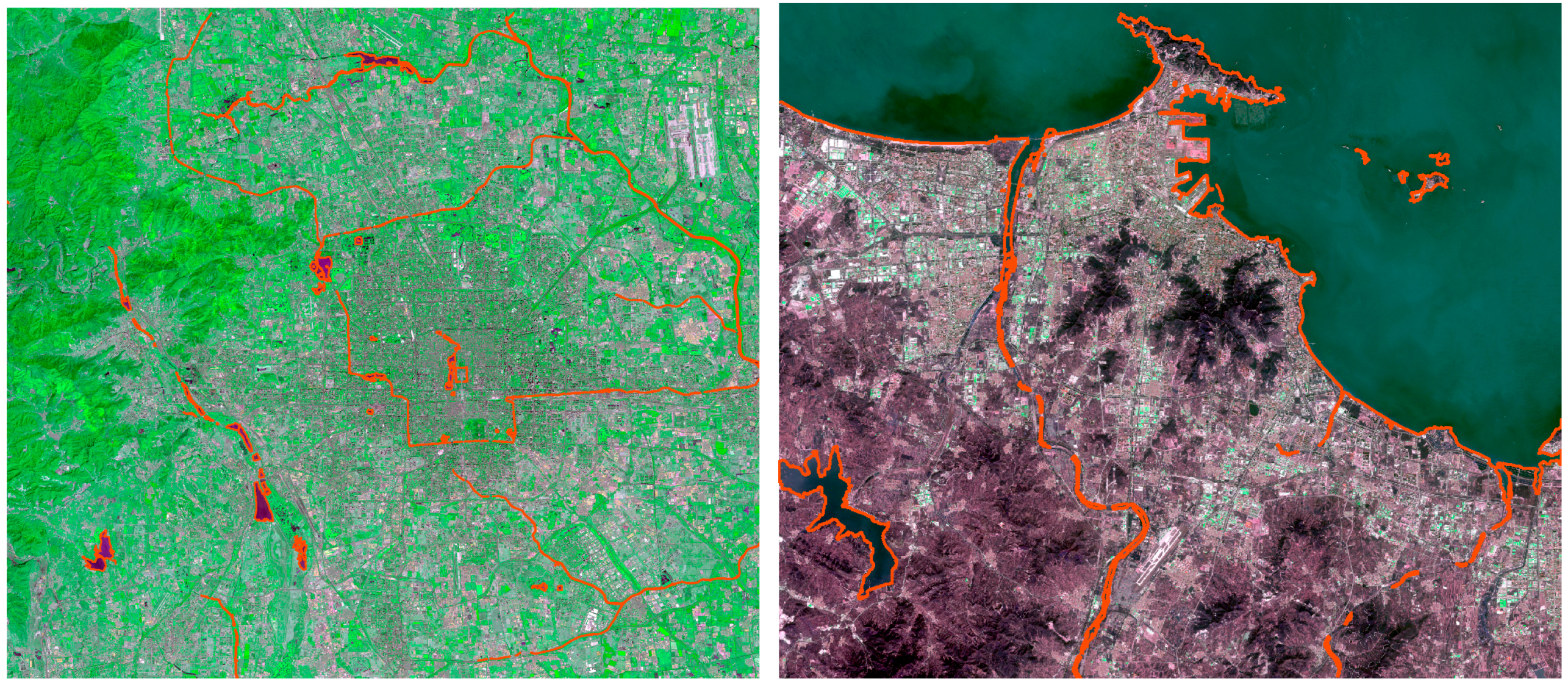
This study, which focuses on large lakes, wide rivers, and coastal areas, obtains the boundary position from different water maps by comparison with a manual drawing (Figure 11). Table 3 lists the boundary accuracy from different water indices in which the NDWI-based method yields good results in both study areas. FPC obtained a relatively unsatisfying result in coastal Yantai. MRSB barely yielded an acceptable boundary recognition rate, which is only slightly better than the original MNDWI (20 m). NDWI (10 m) s truly restricted considering the low extraction rate in downtown Beijing, however, it obtained the second-best result in coastal Yantai.
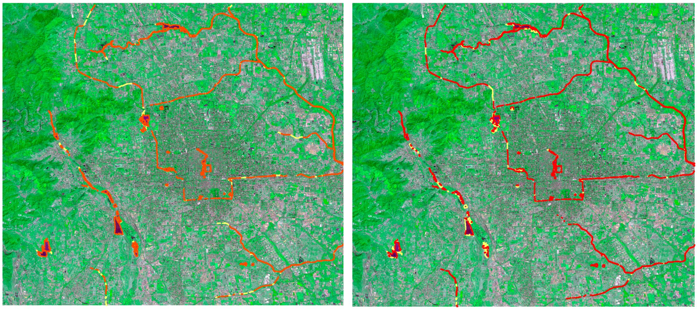
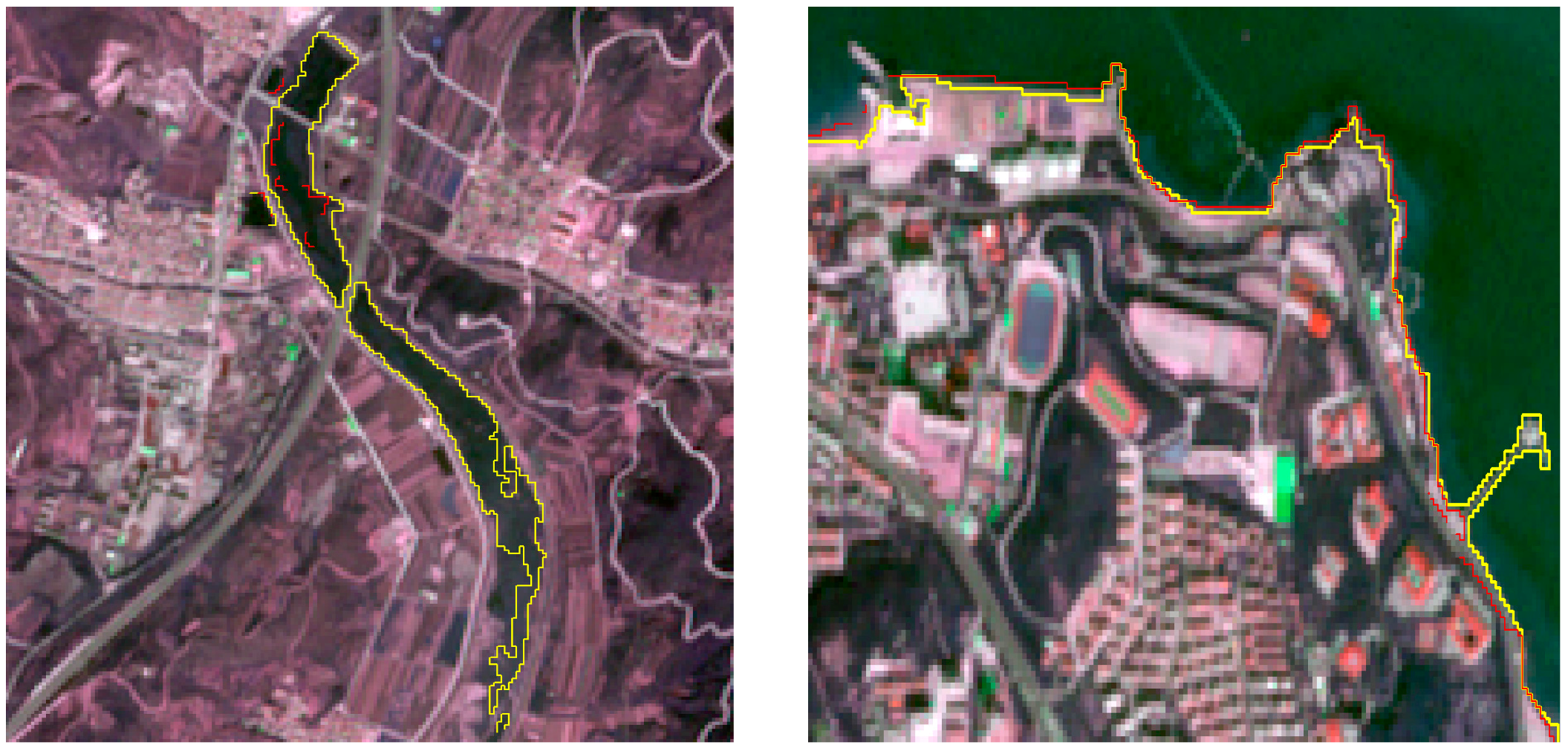
Figure 12 shows the accurate boundaries of three band-like sharpening approaches through intersection judgment with manual drawing. The red lines show the results from FPC (left) and MRSB (right), whereas the yellow lines show the results from NDWII. FPC and MRSB exhibit a more severe fracture phenomenon, whereas NDWII can fill in the breaking parts to a certain degree. Figure 13 shows the boundary recognition in some typical sub-areas in Yantai via NDWII (yellow lines) and NDWI (10 m) (red lines). For the lake, to a less marked degree, NDWI (10 m) fails to detect the object, whereas NDWII succeeds in tracking most of the boundary. For the coastal line, NDWII demonstrates superiority in raised areas, whereas NDWI is not functional.
4. Discussion
The water index is used to enhance the separation and difference between water and non-water areas, as well as to avoid spectral similarity between dark shadow and roads. The analysis of the MNDWI image and the final water map demonstrates the effectiveness of the proposed NDWII-based pan-like sharpening approach.
Image sharpening is used to merge high spatial and multispectral information. The proposed NDWI-based sharpening approach can deal with the water information. In general, this contention can be used in vegetation recognition with an Normalized Difference Vegetation Index (NDVI) image to sharpen the specific red edge bands in Sentinel-2 MSI imagery. Similarly, burned land can be highlighted by the Burn Area Index (BAI) [35] with red and NIR bands (Equation (5)). The Normalised Burn Ratio (NBR) (Equation (6)) [36] and improved NBR thermal 1 (Equation (7)) [37] are applied with relatively low-resolution SWIR and thermal bands, thereby improving separability between burned and unburned land. Similar BAI-based image sharpening may outstand burned land with high spatial resolution and multispectral information.
The objective of this study is to explore the most feasible high-resolution band with which to sharpen the low-resolution SWIR band of Sentinel-2 imagery to enhance water information and extract water bodies. To prove the effectiveness of the proposed NDWI-based sharpening approach, spectral information segmentation based on water indices was used to map water bodies and compare the results with different inputted high spatial resolution bands. Only spectral information was utilised; that is, accuracy depended on the results of water indices and the adjusted threshold. The water map was significantly influenced by dark shadows and road areas, in which the spectral value is mixed with water bodies in the MNDWI image. Feyisa’s [38] Automated Water Extraction Index (AWEI) included two indices: AWEInsh (Equation (3)) is mainly used in areas with dark surfaces and AWEIsh (Equations (8) and (9)) is primarily designed to remove shadow pixels. These two indices are combined to overcome shadow in urban areas. Although a few other approaches are available, such as mixture pixel and machine learning, exploring other features, apart from spectral information, is important. In addition, although most existing shadow detection approaches are more suitable for very high-resolution images [39], building a shadow detection method can be introduced to address the limitations of the dark building shadow effect [15].
The detection of a whole river is fairly difficult because of the small width, the presence of vegetation, and the impurity of the water. A part of the river is not detected, in which the spectral value is considerably mixed. Thus, a merging of the disconnected line segments and filling in of the gaps is expected. When similar spectral values between the water and its neighbourhood are considered, a possible approach may be integration with the decomposition of mixed pixels to find the best track of the open areas. Furthermore, the contextual information [40] may help the feature connection process.
5. Conclusions
The launch of the Sentinel-2 satellite has not only provided moderate-resolution remote sensing imagery, but has also improved data quality with its free download service, thereby expanding the application of the traditional moderate-resolution remote sensing imagery.
In this research, our main objective was to explore the effectiveness and optimal choice of pan-like high-resolution bands to sharpen SWIR bands and thus obtain enhanced water index images. The proposed approach based on the NDWI band was determined to be the most feasible with regard to the separability of water bodies in the images of water indices and in obtaining the most accurate water maps. To achieve automation, valley bottom-based threshold adjustment was introduced for water threshold selection. Although this adjustment may not be optimal, it provides the universal standard for water mapping with different water indices.
The sharpened MNDWI-based water maps significantly improved the Kappa coefficient by nearly 0.3 and the boundary index to over 90% in downtown Beijing compared with conventional NDWI (10 m)- and MNDWI (20 m)-based approaches. For the coastal Yantai study area, conventional NDWI (10 m) obtained good classification and boundary position accuracy, whereas the MNDWI (20 m)-, FPC-, and MRSB-based MNDWI approaches yielded low accuracy, particularly for the boundary index. Nevertheless, the proposed NDWII method also obtained the best water extraction result, which used NDWI as a pan-like band to enhance the SWIR spatial information.
In conclusion, the proposed NDWII-based pan-like band can improve water extraction for Sentinel-2 MSI imagery. It can be integrated into a machine learning technique and mixed pixel decomposition theory to improve the results obtained in this study. Moreover, the index concept-based pan-like construction can be used to enhance certain object information as vegetation red edge bands and other object indices calculated as BAI.
Acknowledgments
This work has been supported by the National Science Foundation of China under Grant No. 61379032, by the Science Foundation of Key Laboratory in Software Engineering of Yunnan Province under Grant No. 2017SE205. This research is supported by China Scholarship Council (Grant CSC No. 201504490008).
Author Contributions
X.Y. and S.Z. conceived and designed the experiments; X.Y., X.Q., and L.L. performed the experiments and analyzed the data; X.Y., X.Q., and N.Z. wrote the paper.
Conflicts of Interest
The authors declare no conflict of interest.
Abbreviations
The following abbreviations are used in this manuscript:
| MSI | Multispectral Instrument |
| NIR | Near InfraRed |
| SWIR | Short-Wavelength InfraRed |
| TOA | Top-Of-the-Atmosphere |
| NDWI | Normalised Difference Water Index |
| MNDWI | Modified Normalised Difference Water Index |
| PCA | principal component analysis |
| NDWII | NDWI Image based pan-like sharpening method |
| MRSB | Most Related Single Band based pan-like sharpening method |
| FPC | PCA First Principal Component based pan-like sharpening method |
| HSV | Hue Saturation Value |
| BI | Boundary Index |
| AWEI | Automated Water Extraction Index |
| BAI | Burn Area Index |
| NBR | Normalised Burn Ratio |
References
- Klemenjak, S.; Waske, B.; Valero, S.; Chanussot, J. Automatic detection of rivers in high-resolution SAR data. IEEE J. Sel. Top. Appl. Earth Obs. Remote Sens. 2012, 5, 1364–1372. [Google Scholar] [CrossRef]
- Brisco, B.; Short, N.; Sanden, J.V.D.; Landry, R.; Raymond, D. A semi-automated tool for surface water mapping with RADARSAT-1. Can. J. Remote Sens. 2009, 35, 336–344. [Google Scholar] [CrossRef]
- Canaz, S.; Karsli, F.; Guneroglu, A.; Dihkan, M. Automatic boundary extraction of inland water bodies using LiDAR data. Ocean Coast. Manag. 2015, 118, 158–166. [Google Scholar] [CrossRef]
- Sharma, R.C.; Tateishi, R.; Hara, K.; Nguyen, L.V. Developing superfine water index (SWI) for global water cover mapping using MODIS data. Remote Sens. 2015, 7, 13807–13841. [Google Scholar] [CrossRef]
- Lu, S.; Jia, L.; Zhang, L.; Wei, Y.; Baig, M.H.A.; Zhai, Z.; Zhang, G. Lake water surface mapping in the Tibetan Plateau using the MODIS MOD09Q1 product. Remote Sens. Lett. 2016, 8, 224–233. [Google Scholar] [CrossRef]
- Sarp, G. Spectral and spatial quality analysis of pan-sharpening algorithms: A case study in Istanbul. Eur. J. Remote Sens. 2014, 47, 19–28. [Google Scholar] [CrossRef]
- Huang, C.; Chen, Y.; Wu, J.; Li, L.; Liu, R. An evaluation of Suomi NPP-VIIRS data for surface water detection. Remote Sens. Lett. 2015, 6, 155–164. [Google Scholar] [CrossRef]
- Zhang, Y.; Gao, J.; Wang, J. Detailed mapping of a salt farm from Landsat TM imagery using neural network and maxi-mum likelihood classifiers: A comparison. Int. J. Remote Sens. 2007, 28, 2077–2089. [Google Scholar] [CrossRef]
- Chen, C.; Qin, Q.; Zhang, N.; Li, J.; Chen, L.; Wang, J.; Qin, X.; Yang, X. Extraction of bridges over water from high-resolution optical remote-sensing images based on mathematical morphology. Int. J. Remote Sens. 2014, 35, 3664–3682. [Google Scholar] [CrossRef]
- Zeng, C.; Bird, S.; Luce, J.J.; Wang, J. A natural-rule-based-connection (NRBC) method for river network extraction from high-resolution imagery. Remote Sens. 2015, 7, 14055–14078. [Google Scholar] [CrossRef]
- Zhou, Y.; Luo, J.; Shen, Z.; Hu, X.; Yang, H. Multiscale water body extraction in urban environments from satellite images. IEEE J. Sel. Top. Appl. Earth Obs. Remote Sens. 2014, 7, 4301–4312. [Google Scholar] [CrossRef]
- Xie, H.; Luo, X.; Xu, X.; Pan, H.; Tong, X. Automated Subpixel Surface Water Mapping from Heterogeneous Urban Environments Using Landsat 8 OLI Imagery. Remote Sens. 2016, 8. [Google Scholar] [CrossRef]
- Zhou, Y.; Dong, J.; Xiao, X.; Xiao, T.; Yang, Z.; Zhao, G.; Zou, Z.; Qin, Y. Open Surface Water Mapping Algorithms: A Comparison of Water-Related Spectral Indices and Sensors. Water 2017, 9. [Google Scholar] [CrossRef]
- Fisher, A.; Flood, N.; Danaher, T. Comparing Landsat water index methods for automated water classification in eastern Australia. Remote Sens. Environ. 2016, 175, 167–182. [Google Scholar] [CrossRef]
- Yao, F.; Wang, C.; Dong, D.; Luo, J.; Shen, Z.; Yang, K. High-resolution mapping of urban surface water using ZY-3 multi-spectral imagery. Remote Sens. 2015, 7, 12336–12355. [Google Scholar] [CrossRef]
- Yang, L.; Tian, S.; Yu, L.; Ye, F.; Qian, J.; Qian, Y. Deep learning for extracting water body from Landsat imagery. Int. J. Innov. Comput. Inf. Control 2015, 11, 1913–1929. [Google Scholar]
- Ko, B.C.; Kim, H.H.; Nam, J.Y.; Lamberti, F. Classification of Potential Water Bodies Using Landsat 8 OLI and a Combination of Two Boosted Random Forest Classifiers. Sensors 2015, 15, 13763–13777. [Google Scholar] [CrossRef] [PubMed]
- Singh, K.; Ghosh, M.; Sharma, S.R. WSB-DA: Water Surface Boundary Detection Algorithm Using Landsat 8 OLI Data. IEEE J. Sel. Top. Appl. Earth Obs. Remote Sens. 2016, 9, 363–368. [Google Scholar] [CrossRef]
- Jiang, H.; Feng, M.; Zhu, Y.; Lu, N.; Huang, J.; Xiao, T. An automated method for extracting rivers and lakes from Landsat imagery. Remote Sens. 2014, 6, 5067–5089. [Google Scholar] [CrossRef]
- Drusch, M.; Del Bello, U.; Carlier, S.; Colin, O.; Fernandez, V.; Gascon, F.; Meygret, A. Sentinel-2: ESA’s optical high-resolution mission for GMES operational services. Remote Sens. Environ. 2012, 120, 25–36. [Google Scholar] [CrossRef]
- Vrabel, J. Multispectral imagery band sharpening study. Photogramm. Eng. Remote Sens. 1996, 62, 1075–1084. [Google Scholar]
- Du, Y.; Zhang, Y.; Ling, F.; Wang, Q.; Li, W.; Li, X. Water bodiesʼ mapping from Sentinel-2 imagery with Modified Normalized Difference Water Index at 10-m spatial resolution produced by sharpening the SWIR band. Remote Sens. 2016, 8, 354–373. [Google Scholar] [CrossRef]
- Xu, H. Modification of normalised difference water index (NDWI) to enhance open water features in remotely sensed imagery. Int. J. Remote Sens. 2006, 27, 3025–3033. [Google Scholar] [CrossRef]
- Chen, C.; Qin, Q.; Chen, L.; Zheng, H.; Fa, W.; Ghulam, A.; Zhang, C. Photometric correction and reflectance calculation for lunar images from the Chang’E-1 CCD stereo camera. J. Opt. Soc. Am. A 2015, 32, 2409–2422. [Google Scholar] [CrossRef] [PubMed]
- McFeeters, S.K. The use of the Normalized Difference Water Index (NDWI) in the delineation of open water features. Int. J. Remote Sens. 1996, 17, 1425–1432. [Google Scholar] [CrossRef]
- Wang, Q.; Shi, W.; Atkinson, P.M.; Pardo-Igúzquiza, E. A new geostatistical solution to remote sensing image downscaling. IEEE Trans. Geosci. Remote Sens. 2016, 54, 386–396. [Google Scholar] [CrossRef]
- Huang, C.; Chen, Y.; Zhang, S.; Li, L.; Shi, K.; Liu, R. Surface water mapping from suomi NPP-VIIRS imagery at 30 m resolution via blending with Landsat data. Remote Sens. 2016, 8. [Google Scholar] [CrossRef]
- Laben, C.A.; Brower, B.V. Process for Enhancing the Spatial Resolution of Multispectral Imagery using PanSharpening. Available online: http://www.google.com/patents/US6011875 (accessed on 12 June 2017).
- eCognition Developer 9. Available online: http://www.ecognition.com/suite/ecognition-developer (accessed on 12 June 2017).
- Ji, L.; Zhang, L.; Wylie, B. Analysis of dynamic thresholds for the Normalized Difference Water Index. Photogramm. Eng. Remote Sens. 2009, 75, 1307–1317. [Google Scholar] [CrossRef]
- Zheng, Y.; Jeon, B.; Xu, D.; Wu, Q.M.; Zhang, H. Image segmentation by generalized hierarchical fuzzy C-means algorithm. J. Intell. Fuzzy Syst. 2015, 28, 961–973. [Google Scholar]
- Sezgin, M. Survey over image thresholding techniques and quantitative performance evaluation. J. Electron. Imaging 2004, 13, 146–168. [Google Scholar]
- Otsu, N. A threshold selection method from gray-level histograms. Automatica 1975, 11, 23–27. [Google Scholar] [CrossRef]
- Yen, J.C.; Chang, F.J.; Chang, S. A New Criterion for Automatic Multilevel Thresholding. IEEE Trans. Image Process. 1995, 4, 370–378. [Google Scholar] [PubMed]
- Chuvieco, E.; Martin, M.P.; Palacios, A. Assessment of Different Spectral Indices in the Red-Near-Infrared Spectral Domain for Burned Land Discrimination. Remote Sens. Environ. 2002, 23, 2381–2396. [Google Scholar] [CrossRef]
- Key, C.N.; Benson, N. Landscape Assessment: Remote Sensing of Severity, the Normalized Burn Ratio; and Ground Measure of Severity, the Composite Burn Index. In FIREMON: Fire Effects Monitoring and Inventory System; USDA: Fort Collins, CO, USA, 2005. [Google Scholar]
- Holden, Z.A.; Smith, A.M.S.; Morgan, P.; Rollins, M.G.; Gessler, P.E. Evaluation of Novel Thermally Enhanced Spectral Indices for Mapping Fire Perimeters and Comparisons with Fire Atlas Data. Int. J. Remote Sens. 2005, 26, 4801–4808. [Google Scholar] [CrossRef]
- Feyisa, G.L.; Meilby, H.; Fensholt, R.; Proud, S.R. Automated Water Extraction Index: A new technique for surface water mapping using Landsat imagery. Remote Sens. Environ. 2013, 140, 23–35. [Google Scholar] [CrossRef]
- Adeline, K.R.M.; Chen, M.; Briottet, X.; Pang, S.K.; Paparoditis, N. Shadow detection in very high spatial resolution aerial images: A comparative study. ISPRS J. Photogramm. Remote Sens. 2013, 80, 21–38. [Google Scholar] [CrossRef]
- Zhou, Z.; Wang, Y.; Wu, Q.J.; Yang, C.N.; Sun, X. Effective and efficient global context verification for image copy detection. IEEE Trans. Inf. Forensics Secur. 2017, 12, 48–63. [Google Scholar] [CrossRef]
Figure 1.
Workflow of the band sharpening and water mapping.

Figure 2.
Study area and imagery materials. The study area is located in urban area of Beijing and Yantai, China. The Sentinel-2 Multispectral Instrument (MSI) imagery is shown with true-colour composite of Red, Green, and Blue bands of the raw image data.
Figure 2.
Study area and imagery materials. The study area is located in urban area of Beijing and Yantai, China. The Sentinel-2 Multispectral Instrument (MSI) imagery is shown with true-colour composite of Red, Green, and Blue bands of the raw image data.

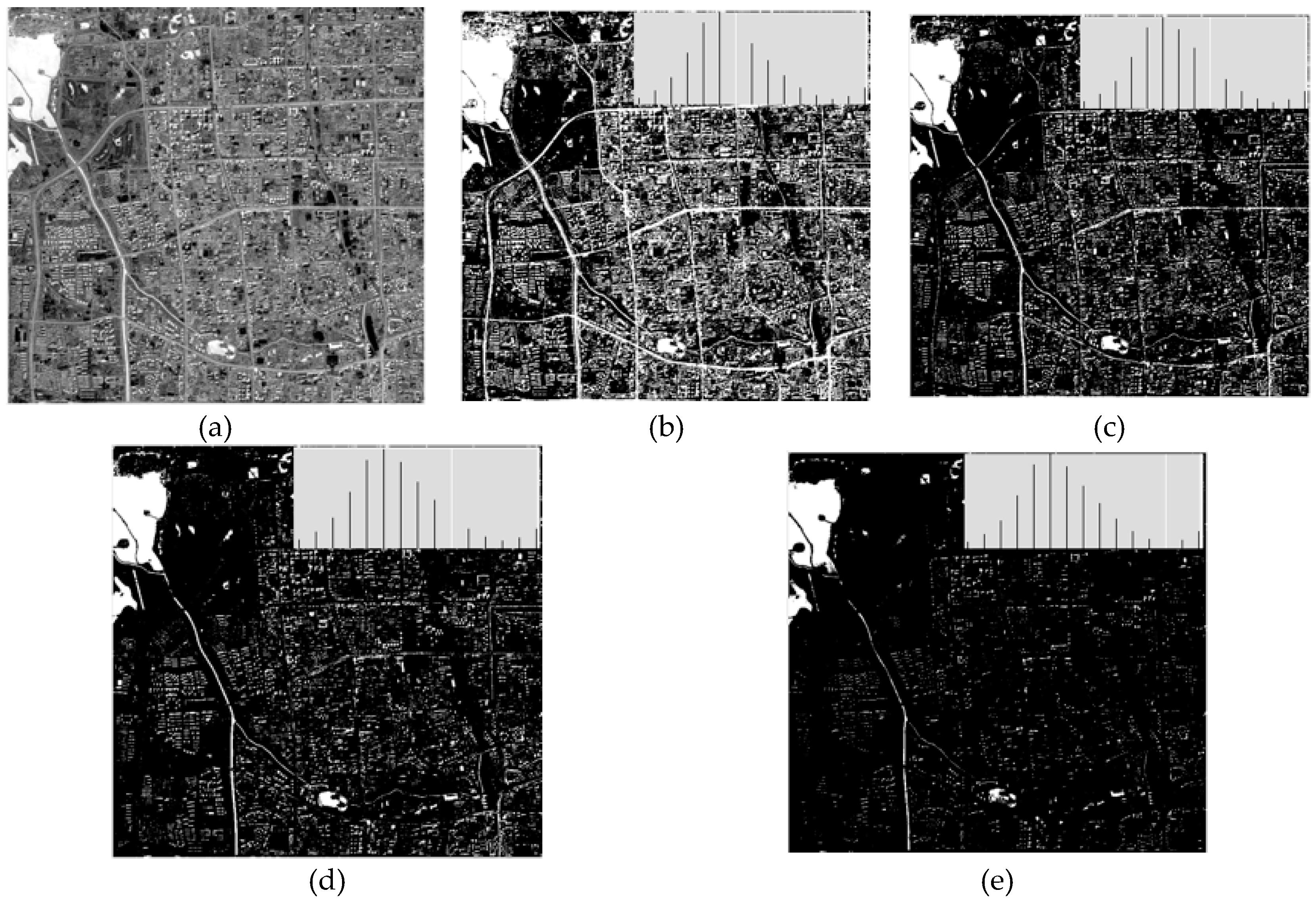
Figure 3.
Different segmentation results and adjusted thresholds that used several typical threshold adjustment approaches, (a) Water index image; (b) Otsu’s method; (c) Entropy threshold; (d) Yen’s method [34]; (e) Valley bottom. The sub-image in the right-up (b–e) shows the grey histogram of the image and the white line indicates the obtained threshold.

Figure 4.
Pixel distribution between water and non-water areas.

Figure 5.
The red line represents the reference river bank line, and the orange area is its buffer area. Part of the extracted river boundary (blue) is in accordance with the reference, whereas the green part is an inaccurate boundary. The boundary index (BI) refers to the ratio between the lengths of the blue and red lines.

Figure 6.
MNDWI images (upper) and pixel-wise water extraction (lower) at 10 m resolution using three pan-like high spatial resolution bands.
Figure 6.
MNDWI images (upper) and pixel-wise water extraction (lower) at 10 m resolution using three pan-like high spatial resolution bands.

Figure 7.
The theoretical separation between water and non-water areas. The blue and red normal distribution represents the water indices image values of water pixels and non-water pixels.
Figure 7.
The theoretical separation between water and non-water areas. The blue and red normal distribution represents the water indices image values of water pixels and non-water pixels.

Figure 8.
Local pixel value changes in different images of the water indices. For the three different approaches, the obtained MNDWI image can return two thresholds, shown as the red line and green line in the pixel value change curve. The red line means to obtain accurate water pixels without noise, while the green lines corresponds to extraction of the whole water pixels in spite of some error pixels. For the proposed NDWII approach, the red line and green line tend to be coincide, which means it can nearly extract all the water pixels with little noise.

Figure 9.
Final surface water maps (blue blocks) utilizing different approaches in Beijing. The reference image is the manual drawing by visual interpretation process.
Figure 9.
Final surface water maps (blue blocks) utilizing different approaches in Beijing. The reference image is the manual drawing by visual interpretation process.

Figure 10.
Final surface water maps (blue blocks) utilizing different approaches in Yantai. The reference image is the manual drawing by visual interpretation process. The red boundary in the reference excludes the ocean areas in the accuracy assessment, because such a large area of clear water pixels in ocean areas can always lead to a high extraction rate.

Figure 11.
Manual drawing of typical water bodies in the study areas (left: Beijing; right: Yantai. The image is true color synthesis with band 4, 3, & 2) to assess the boundary index.
Figure 11.
Manual drawing of typical water bodies in the study areas (left: Beijing; right: Yantai. The image is true color synthesis with band 4, 3, & 2) to assess the boundary index.

Figure 12.
The comparative boundary extraction results utilizing different pan-like sharpening approaches from the Sentinel-2 image (true color synthesis) of Beijing. The red lines denote the results from the FPC (left) and MRSB (right) approaches, whereas the yellow lines indicate the result from the MNDWII approach.

Figure 13.
The comparative boundary extraction results of the proposed NDWII method and traditional NDWI method from the Sentinel-2 image (true color synthesis) of Yantai. The yellow lines present the result using the proposed NDWII method, whereas the red lines show the results using traditional NDWI (10 m).


Table 1.
Correlation coefficient between RGB/NIR and SWIR bands in the study area.
| Band (Study Area) | Blue | Green | Red | NIR |
|---|---|---|---|---|
| SWIR 1 (Beijing) | 0.305210 | 0.873271 | 0.153695 | 0.254547 |
| SWIR 2 (Beijing) | 0.663644 | 0.416851 | 0.660396 | 0.686762 |
| SWIR 1 (Yantai) | 0.483044 | 0.271207 | 0.682017 | 0.989808 |
| SWIR 2 (Yantai) | 0.609192 | 0.420959 | 0.799635 | 0.945101 |
Table 2.
Water mapping accuracy assessment results on the Sentinel-2 image.
| Study Area | Approach | PA | UA | OA | Kappa |
|---|---|---|---|---|---|
| Beijing | NDWII | 87.61% | 92.36% | 99.39% | 0.910 |
| FPC | 91.09% | 93.68% | 99.46% | 0.921 | |
| MRSB | 82.06% | 97.94% | 99.29% | 0.889 | |
| MNDWI (20 m) | 58.65% | 98.15% | 97.03% | 0.645 | |
| NDWI (10 m) | 68.05% | 98.41% | 98.81% | 0.799 | |
| Yantai | NDWII | 92.78% | 87.93% | 99.00% | 0.878 |
| FPC | 82.94% | 93.47% | 98.96% | 0.863 | |
| MRSB | 81.69% | 94.51% | 98.95% | 0.860 | |
| MNDWI (20 m) | 87.29% | 88.39% | 98.72% | 0.839 | |
| NDWI (10 m) | 87.97% | 90.77% | 99.04% | 0.878 |
Note: The accuracy assessments for Yantai eliminate the homogeneous sea areas, which dramatically affect the real accuracy of the urban land surface water extraction. Only inland water and the coastal line is considered, as shown in the red lines for the reference image in the Figure 10.
Table 3.
The boundary index utilizing different water indices.
| NDWII | FPC | MRSB | MNDWI (20 m) | NDWI (10 m) | |
|---|---|---|---|---|---|
| Beijing | 0.966 | 0.942 | 0.843 | 0.815 | 0.377 |
| Yantai | 0.928 | 0.807 | 0.799 | 0.775 | 0.863 |
© 2017 by the authors. Licensee MDPI, Basel, Switzerland. This article is an open access article distributed under the terms and conditions of the Creative Commons Attribution (CC BY) license (http://creativecommons.org/licenses/by/4.0/).
Share and Cite
MDPI and ACS Style
Yang, X.; Zhao, S.; Qin, X.; Zhao, N.; Liang, L. Mapping of Urban Surface Water Bodies from Sentinel-2 MSI Imagery at 10 m Resolution via NDWI-Based Image Sharpening. Remote Sens. 2017, 9, 596. https://doi.org/10.3390/rs9060596
AMA Style
Yang X, Zhao S, Qin X, Zhao N, Liang L. Mapping of Urban Surface Water Bodies from Sentinel-2 MSI Imagery at 10 m Resolution via NDWI-Based Image Sharpening. Remote Sensing. 2017; 9(6):596. https://doi.org/10.3390/rs9060596
Chicago/Turabian StyleYang, Xiucheng, Shanshan Zhao, Xuebin Qin, Na Zhao, and Ligang Liang. 2017. "Mapping of Urban Surface Water Bodies from Sentinel-2 MSI Imagery at 10 m Resolution via NDWI-Based Image Sharpening" Remote Sensing 9, no. 6: 596. https://doi.org/10.3390/rs9060596
Note that from the first issue of 2016, this journal uses article numbers instead of page numbers. See further details here.