CAWRES: A Waveform Retracking Fuzzy Expert System for Optimizing Coastal Sea Levels from Jason-1 and Jason-2 Satellite Altimetry Data

Abstract

This paper presents the Coastal Altimetry Waveform Retracking Expert System (CAWRES), a novel method to optimise the Jason satellite altimetric sea levels from multiple retracking solutions. CAWRES’ aim is to achieve the highest possible accuracy of coastal sea levels, thus bringing measurement of radar altimetry data closer to the coast. The principles of CAWRES are twofold. The first is to reprocess altimeter waveforms using the optimal retracker, which is sought based on the analysis from a fuzzy expert system. The second is to minimise the relative offset in the retrieved sea levels caused by switching from one retracker to another using a neural network. The innovative system is validated against geoid height and tide gauges in the Great Barrier Reef, Australia for Jason-1 and Jason-2 satellite missions. The regional investigations have demonstrated that the CAWRES can effectively enhance the quality of 20 Hz sea level data and recover up to 16% more data than the standard MLE4 retracker over the tested region. Comparison against tide gauge indicates that the CAWRES sea levels are more reliable than those of Sensor Geophysical Data Records (SGDR) products, because the former has a higher (≥0.77) temporal correlation and smaller (≤19 cm) root mean square errors. The results demonstrate that the CAWRES can be applied to coastal regions elsewhere as well as other satellite altimeter missions.

1. Introduction

Increasing demand for accurate sea level anomaly (SLA) data close to the coast has led to a huge development in coastal altimetry and its applications, such as coastal management, long-term monitoring of coastal dynamics and storm surge studies.

Satellite radar altimeters measure the range, a distance between satellite and the nadir surface, by retrieving the two-way travel time of radar short pulses sent to and reflected from the ocean surface. The SLA is referenced to a mean sea surface and can be then derived from the range and satellite orbit. The reflected signal is called the ‘waveform’ and represents the time evolution of the reflected power as the radar signal hits the surface. Waveforms over a homogeneous ocean surface (e.g., open ocean without land interference) can generally be described by Brown [1] model. It features a sharp leading edge up to the maximum value of the amplitude, followed by a gently sloping plateau known as the trailing edge.

In the proximity of land, conventional Ku-band altimetry data usually requires a complex sequence of processing steps to get usable information about the SLAs. This is because the waveform signals are contaminated by land or calm waters (cf. [2,3]) and the corrections are less accurate over the coastal regime. Through processing, better estimates of the range parameter (that is related to the SLA), and the geophysical corrections (particularly the wet tropospheric, dynamic atmospheric and ocean tide corrections) can be obtained. The range estimates can be optimised through a ground re-processing protocol called ‘waveform retracking’ (cf. [4,5,6,7,8,9,10,11]), which was routinely conducted over global oceans to improve the accuracy of altimetry measurements. The state-of-the-art about retracking and geophysical corrections can be found in the book Coastal Altimetry by Vignudelli et al. [12], and in particular in the chapter by Gommenginger et al. [13] and Andersen and Scharroo [14].

In recent years, many initiatives were undertaken to provide data upgrades (e.g., PISTACH and PEACHI products) and new retracking strategies over coastal regions (e.g., [8,15,16,17,18,19,20,21]). As a result, the altimetry no-data gap was reduced to ~10 km to the coastline. However, within ~10 km from the coastline, the improvement of altimetry data is still challenging due to the complex nature of coastal topography and calm sea states.

When attempting to extract precise sea levels from corrupted waveforms near shore, several researchers (cf. [5,22,23]) suggest combining multiple retracking algorithms for dealing with various waveform shapes. However, there is a lack of clear recommendations and guidelines on which retracker should be used under various conditions (cf. [24]). Several methods were proposed regarding the selection of the optimal retracker for reprocessing various waveform patterns. The rule-based expert system was found useful for proposing dedicated retrackers based on waveform characteristics [5,23]. Because the system is mainly based on physical features of waveforms, it is crucial to accurately classify altimetric waveforms into different classes, so that they can be assigned to corresponding retrackers. It is also important to minimise the discontinuity of the retrieved geophysical parameters when switching retrackers from the open ocean to the coast, or vice versa. One cannot simply switch from one retracker to another due to the relative sea level offsets between them (cf. [8,25,26]).

In this study, we initiate a novel method to retrieve precise SLAs from multiple retracking solutions through a Coastal Altimetry Waveform Retracking Expert System (CAWRES). The CAWRES is designed to optimise the estimation of SLAs by selecting the optimal retracker via a fuzzy expert system and to provide a seamless transition from the open ocean to coastlines (or vice versa) when switching retrackers via a neural network approach. The parameter of interest is the SLA that refers to the mean sea surface rather than the geoid because the geoid is inaccurate at high frequency wavelengths [27].

The article is organised as follows: the study area and data are described in Section 2; the development of the CAWRES is described in Section 3; the consideration and initial testing of CAWRES is discussed in Section 4; the performance of CAWRES in the region of the Great Barrier Reef in Australia, against geoid height and tide gauge is provided in Section 5; and conclusions and recommendations are provided in Section 6.

2. Study Area and Data

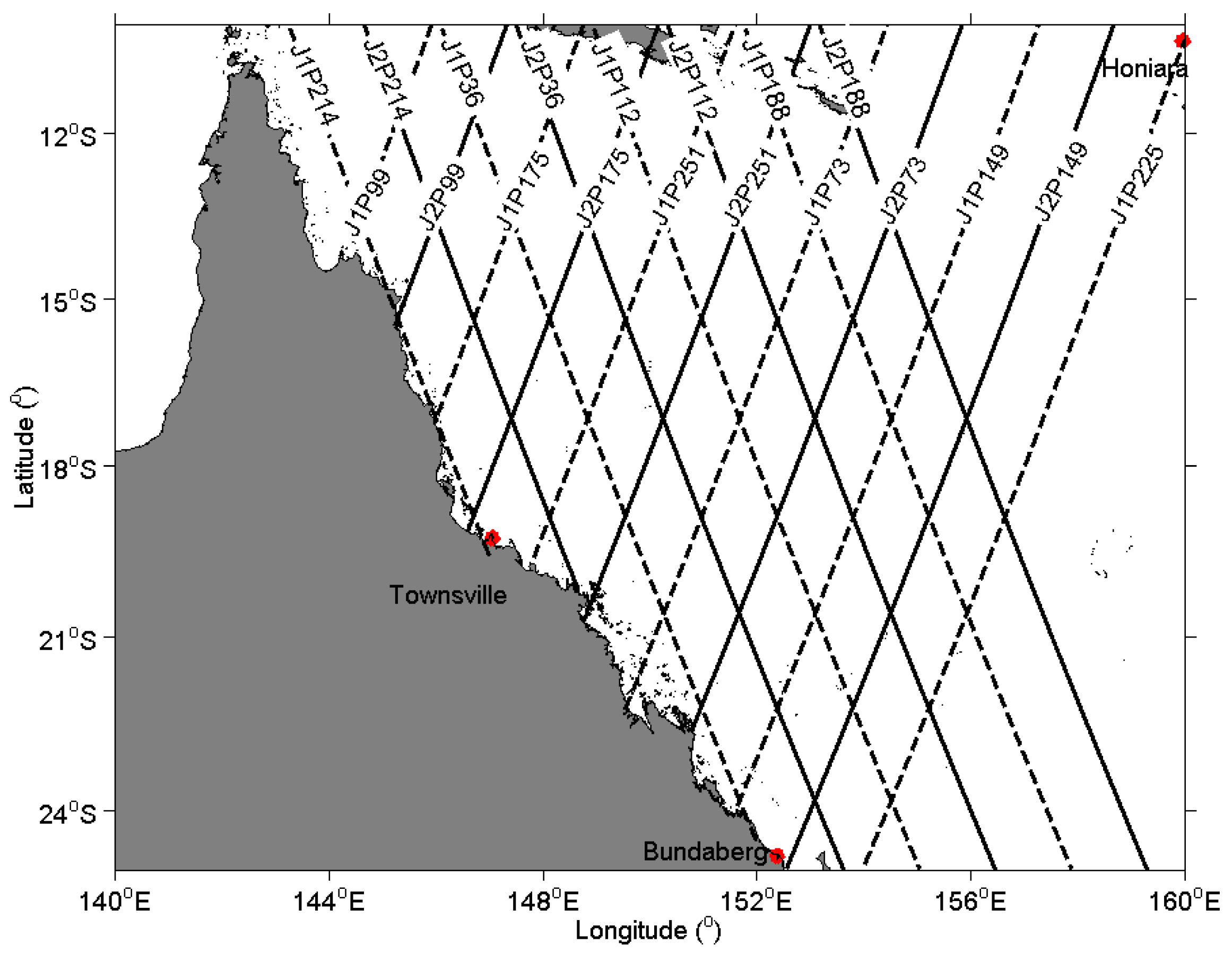
The region of the Great Barrier Reef in Australia (Figure 1) is chosen as the study area due to it’s unique morphology characterised by distinct basins, and sub-basins surrounded by a complex shoreline with specific oceanographic features. Situated in the Coral Sea off the coast of Queensland, the Great Barrier Reef is the world’s largest reef system. It is ~2600 km in length and is composed of ~3000 individual reefs and ~900 islands. It experiences a tropical climate with a severe tropical cyclone season during the austral summer. Data selected in this area can capture diverse waveform patterns due to the spatial complexity of the topography and the temporal variability of coastal sea states.

The data used are Jason-1 and Jason-2/OSTM obtained during the tandem mission. The Ku-band 20-Hz 104-sample waveform data are from January 2009 to December 2011, which corresponds to cycles 262 to 370 of Jason-1 and cycles 19 to 143 of Jason-2. Over the Great Barrier Reef, waveforms along five ascending passes (73, 99, 149, 175, and 251) and four descending passes (36, 112, 188, and 214) of both satellites are investigated (Figure 1).

In producing SLAs, environmental and geophysical corrections from Sensor Geophysical Data Record (SGDR) products and the mean sea surface from DTU10 model [28] are applied to the altimeter range. The wet and dry tropospheric corrections are from the European Centre for Medium-Range Weather Forecasts (ECMWF) numerical prediction models, and ionospheric correction is from the General Ionospheric Model Map. The more accurate instrumental radiometer wet correction and dual frequency ionospheric correction are not used because of coastal contamination effects. The ocean tidal signals are removed using a pointwise tide modelling [17] rather than the global ocean tide model, such as FES2004 and GOT4.8, because it better resolves the tidal signals in the study region. The sea state bias correction is not applied because it is not appropriate for waveforms near coasts (cf. [14]). It is applied neither to coastal data to avoid additional error nor to open ocean data to keep consistency of datasets in the area. The corrections were interpolated from 1 Hz to 20 Hz.

The quality and consistency of sea levels derived from CAWRES is compared with geoid height and tide gauges. The geoidal height is based on the Earth Gravitational Model 2008 (EGM2008) with 2.5 min resolution. The tide gauge data are from the University of Hawaii Sea Level Center). It is the hourly sea level data from Townsville (19.25°S, 146.83°E), Bundaberg (24.75°S, 152.42°E), and Honiara (9.44°S, 159.95°E) stations (see Figure 1). The assessment with tide gauge merits to finding both the accuracy and precision of the SLA estimates, while with the geoidal heights, only the precision can be computed.

3. The Development of CAWRES

The CAWRES consists of two major principles. The first is to minimise the relative offset in the retrieved SLAs when switching from one retracker to another using a neural network (Section 4.1.2). The second is to reprocess altimeter waveforms using the optimal retracker based on the analysis from a fuzzy expert system. The CAWRES employs multiple retracking algorithms to reprocess various waveforms near a shore. They are the Brown [1] physical-based retrackers that retrack the full-waveform (cf. [5]) (hereafter called the ‘Ocean Model’ retracker) and sub-waveform (cf. [8]) (hereafter called the ‘Sub-waveform’ retracker), and the modified threshold empirical-based retrackers (cf. [18]) with 10%, 20% and 30% of threshold levels (hereafter called the ‘modthreshold10’, ‘modthreshold20’ and ‘modthreshold30’). These retrackers are prioritised depending on the waveforms shape to optimise the SLA estimation. The system repeatedly retracks waveforms until it finds the optimal retracker based on the analysis from the fuzzy expert system. A retracker is considered as optimal when it produces the highest quality retracked SLAs. Detailed information is provided in Section 3.1.

Unlike other retracking expert systems [5,23] that consider only the information about the physical features (i.e., shapes) of waveforms, CAWRES considers both the shapes of waveforms and the statistical features of retracking results to select the optimal retracker. Thus, CAWRES reduces the risk of assigning the waveform to an inappropriate retracker when the classification procedure is unable to accurately identify the class of corrupted waveforms near coasts. The fuzzy system is used because of its capability to model the ambiguousness that occurs during the evaluation process, which cannot be properly described by the classical decision system (e.g., rule-based expert system) [29].

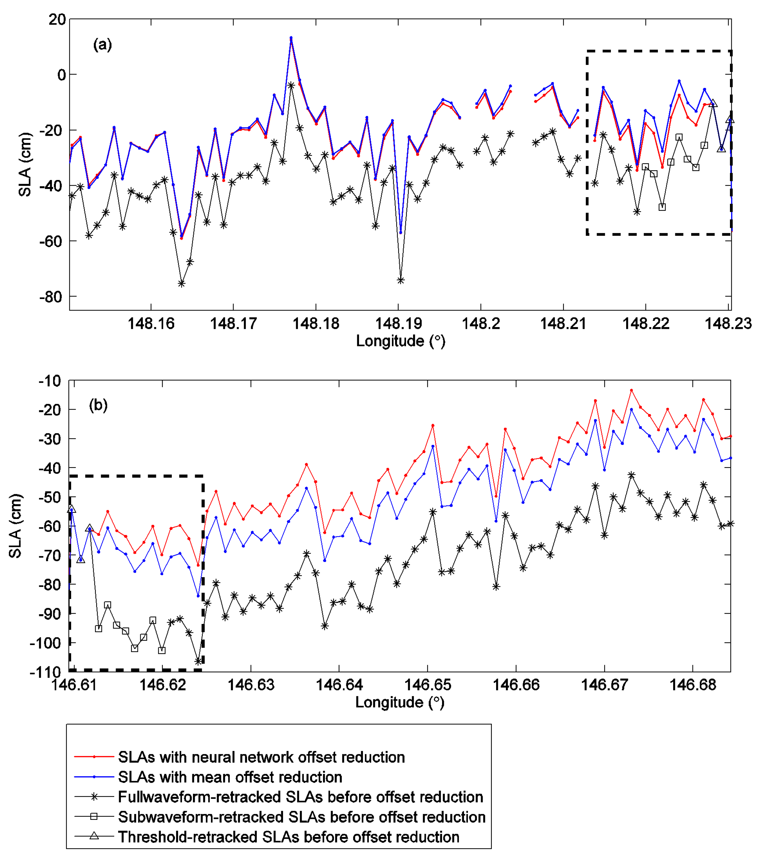
When employing multiple retracking algorithms to improve the estimation of the SLAs in coastal regions, the major problem is that ‘jumps’ may appear in the retracked SLA profiles due to the presence of relative offsets among various retrackers [5,8,19,22,26]. An analysis is reported in Section 4.1.1 to understand the behaviour of the offset among various retrackers. To reduce the offset in retracked SLAs, the novel ideas that exploit a neural network approach are explored because it performs a comprehensive analysis to recognise complex patterns between various retrackers.

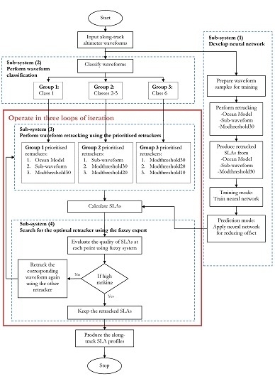
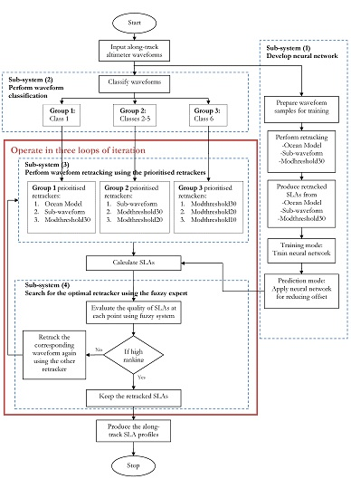
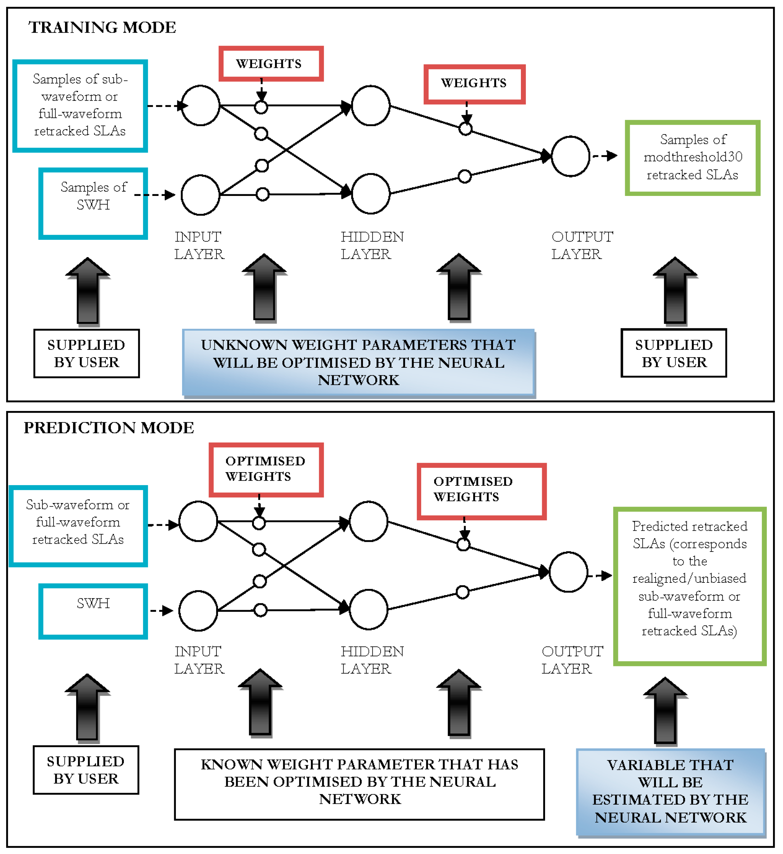
Figure 2 shows the block diagram of the CAWRES. The system consists of four major sub-systems:

• a neural network for producing a seamless transition when switching retrackers (see Section 4.1.2);
• waveform classification for classifying waveforms into several groups (refer to [30]);
• waveform retracking for optimizing the estimation of SLAs; and
• the fuzzy expert system for searching the optimal retracker.

For each satellite track, for example Jason-2 cycle 19 pass 214, the system starts with sub-system (1) by selecting waveform samples and performs the training mode operation in the neural network. The outputs from sub-system (1) are the trained neural network to determine offset 1 (hereafter called the ‘NN1’) and offset 2 (hereafter called the ‘NN2’), which are used later in sub-system (3) to minimise the offsets. The offset 1 is computed between full-waveform and modthreshold30 retrackers and offset 2 is between sub-waveform and modthreshold30 retrackers. These outputs are produced for each individual satellite cycle and pass. It is noted that the offsets between modthreshold30 and modthreshold20 (modthreshold10) retrackers are not computed because our initial study found that the values are insignificant (<5 cm).

In sub-system (2), all waveforms are classified into three groups that are retracked using corresponding retrackers. In sub-systems (3) and (4), the operations are performed in a loop of iterations. The waveform retracking is performed iteratively, from which waveforms in each group are retracked by the n prioritised retrackers where n = 1, 2, 3. A high priority is given to the physical-based retrackers (i.e., Ocean Model and sub-waveform) to reprocess Brown-like waveforms (group 1) and coastal waveforms (group 2) with clear leading edges because they can optimise the geophysical parameters based on a functional form of the reflecting surfaces. The statistical-based retracker is assigned to coastal waveforms (group 3), which appear to have no Brown-like leading edge and contains perturbations in their leading edge. The maximum iteration is three relative to the number of retracking algorithms used in each group.

At the first iteration (n = 1), in sub-system (3), waveforms corresponding to group 1 are retracked by the full-waveform, whereas waveforms corresponding to groups 2 and 3 are retracked by the sub-waveform and modthreshold30 retrackers, respectively. This then produces an along-track retracked SLA profile. To minimise the relative offset among retrackers, NN1 and NN2 from sub-system (1) are used. NN1 is applied to the group that is retracked by the full-waveform, and NN2 is applied to the group that is retracked by the sub-waveform retracker (see Section 4.1.2 for details on NN1 and NN2).

In sub-system (4), the retracked SLAs at each along-track point are subsequently analysed using the fuzzy expert system to quantify the quality of the retracked SLAs (see Section 3.1 for detailed description). When the fuzzy system assesses the quality of the retracked SLA at a point as being high, it keeps the result to produce the final SLA profiles. When its quality is low, the corresponding waveform is retracked again (in sub-system 3) at the second iteration (n = 2), using the second prioritised retracker: sub-waveform for group 1, modthreshold30 and modthreshold20 for groups 2 and 3, respectively. The NN2 is subsequently applied to a point that is retracked by the sub-waveform retracker to realign them to the modthreshold30 retracked SLAs. The quality of retracked SLAs is then assessed again using the fuzzy system in sub-system (4). When the quality is found to be low, the waveform is retracked again at the third iteration (n = 3) using the third prioritised retracker: modthreshold30, modthreshold20 and modthreshold10 for groups 1, 2 and 3, respectively. Retracked SLAs with high quality are kept for the final SLA profiles. However, if no high quality retracked SLA is found at a point after the third iteration, the retracked SLA corresponding to the highest quality retracker is used as the final output of SLAs.

After retracking, the range correction is computed, and subsequently is applied to the altimetry observed range to produce the retracked range. The retracked SLA is computed by subtracting the retracked range from the satellite orbital height, geophysical corrections (e.g., tides, wet and dry tropospheric and ionospheric) and mean sea surface. For the tidal correction, the pointwise tide modelling [31] is applied rather than the global ocean tide models (e.g., GOT 4.8, FES2004 and DTU10) to better remove the shallow water tides (cf. [17]).

Considering that the system in Figure 2 involves complex computations, we examine the execution times of CAWRES using MATLAB implementation for one cycle along different passes (

Table 1. CAWRES execution times for cycle 19 along Jason-2 satellite passes.

Satellite Pass	No. of Waveforms	Total Execution Times (in Seconds)	Averaged Execution Times for a Waveform (in Seconds)
73	5099	290.219	0.057
99	2211	109.753	0.050
149	6099	306.099	0.050
175	3520	184.331	0.052
251	4241	252.085	0.059

). It is processed using a 2.20 GHz i5 CPU, 8 GB Random Access Memory (RAM) and Intel High Definition Graphics 5300. Results shown in Table 1 indicate that the computational time of CAWRES to process a bunch (between 2211 and 6099) of waveforms is ≤306 s with the averaged execution time for an altimetric waveform is ~0.05 s. This is considered reasonable for such a complex system. Note that the implementation of CAWRES in MATLAB has considered several techniques to accelerate the execution times, including the pre-allocation memory and parallel iterations.

Fuzzy Expert System

This section describes about the fuzzy expert system that is applied in subsystem (4) of CAWRES. It is used to evaluate the quality of retracked SLAs because of its capability for integrating information about the statistical features of retracking results, and determining the quality of retracked SLAs accordingly.

After waveform retracking in subsystem (3), the quality of retracking results is computed using a fuzzy expert system. The input variables included in the fuzzy expert system are: (1) the difference of the retracked SLAs from the mean sea surface (Dif_ssh); (2) the differences between two successive retracked SLAs (Dif_ssh_prev1); (3) the difference between a retracked SLAs and the retracked SLA after next (Dif_ssh_prev2); and (4) for the fitting functions of the full-waveform and sub-waveform models, the goodness of fit (r²), which is determined by the correlation level between waveform samples and fitted values, is included. Dif_ssh_prev1 and Dif_ssh_prev2 are included in the system to ensure that the optimal retracker is the one that yields small differences between the previous SLAs. This is because the SLA generally varies smoothly within a certain distance across the ocean surface.

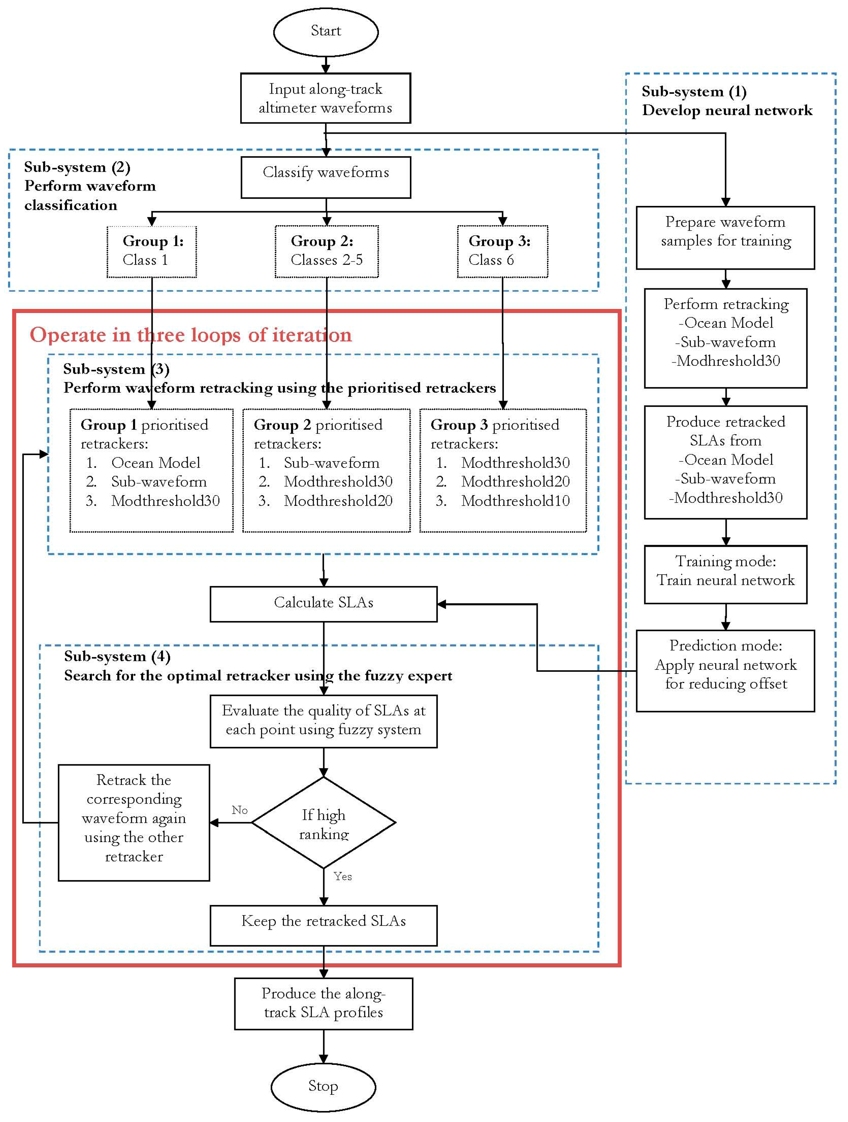
Based on fuzzy logic, the variables can be represented as a set of mathematical principles for knowledge representation based on degrees of membership and degrees of truth. The range of values of a variable represents the universe discourse of that variable. For example, the universe discourse of the linguistic variable r² might have a range between 0 and 1, and may include such fuzzy subsets as poor and good.

Figure 3 shows examples of the fuzzy set of r² and Dif_ssh_prev1. The x-axis represents the universe of discourse, which shows the range of all possible values applicable to the variables r² and Dif_ssh_prev1. The y-axis represents the membership value of the fuzzy set for both variables. The universe of discourse r² consists of two fuzzy sets, poor and good, and the universe of discourse Dif_ssh, Dif_ssh_prev1 and Dif_ssh_prev2 consists of two fuzzy sets, small and large. The characteristics of these fuzzy sets are shown in

Table 2. Characteristics of the fuzzy sets. The range of the universe of discourse is given in units of metre for variables Dif_ssh, Dif_ssh_prev1 and Dif_ssh_prev2.

Universe of Discourse	Range of the Universe of Discourse	Fuzzy Subset
		Subset	Range of Subset *
r2	0–1	Poor	0–0.9
		Good	0.8–1
Dif_ssh	0–10	Small	0–1.5
		Large	1–10
Dif_ssh_prev1	0–100	Small	0–1.5
		Large	1–100
Dif_ssh_prev2	0–100	Small	0–1.5
		Large	1–100

* Range of subset: the fuzzy set allows an overlap in a range of fuzzy subset to represent a fuzzy boundary.

.

Based on the input variables, the system evaluates the quality of retracking results by giving the rank value (between 0 and 10). The rank values between 8 and 10, and 0–7 are of high and low quality, respectively. The evaluation process considers 13 rules. For example,

• If r² is good, and Dif_ssh, Dif_ssh_prev1 and Dif_ssh_prev2 are small, then ranking = high
• If r² is poor, and Dif_ssh, Dif_ssh_prev1 and Dif_ssh_prev2 are large, then ranking = low
• If r² is good, and Dif_ssh, Dif_ssh_prev1 and Dif_ssh_prev2 are large, then ranking = low
• If r² is none, and Dif_ssh, Dif_ssh_prev1 and Dif_ssh_prev2 are large, then ranking = low
• If r² is none, and Dif_ssh, Dif_ssh_prev1 and Dif_ssh_prev2 are small, then ranking = high

The analysis provided by the fuzzy system is used as a basis for determining the optimal retracker near coasts. When it considers the quality of retracked SLA as ‘high ranking’ (value between 8 and 10), the system keeps the retracked SLA, which will be used to produce the final SLA profile. In the case of ‘low ranking’ (value between 0 and 7), the waveform is retracked iteratively using the other retrackers, based on their priority, until a retracked SLA with a ‘high ranking’ is found. If a ‘high ranking’ retracked SLA is not found after all the three retrackers related to the waveform group were applied, the retracked SLA corresponding to the highest ranking retracker is used as the output of the SLA profile.

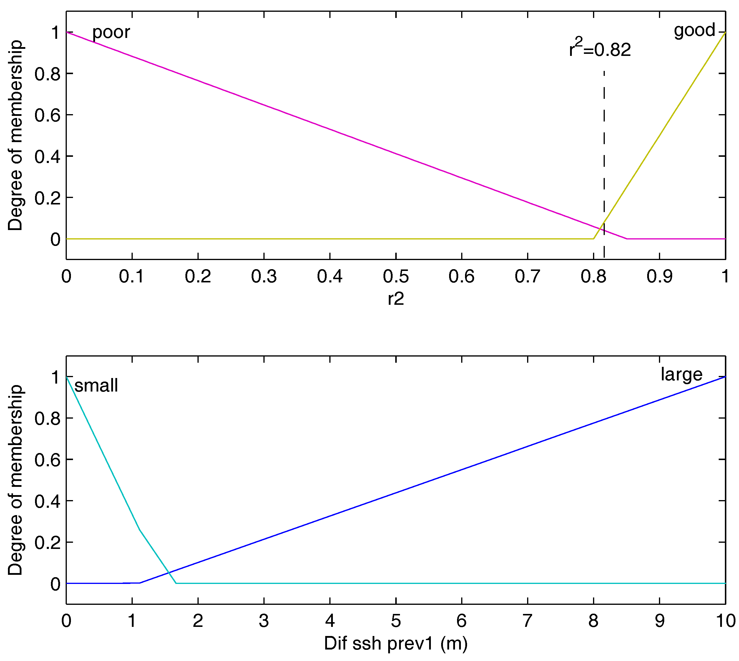
Figure 4 shows an example of retracked SLA profiles (top) and their ranking values (bottom) during iterations 1 to 3. Red circles show problematic areas, where ‘low ranking’ retracked SLAs are found. These areas are iteratively retracked until the optimal retracker is found, which is indicated by the ‘high ranking’ value. In this example, the SLA profile during iteration 1 is found to fluctuate with a standard deviation of 166 cm. However, during iteration 3, the standard deviation reduces to 95 cm. This indicates the fuzzy expert system enhances the SLA precision by proposing the optimal retracker to reprocess waveforms.

4. Considerations and Initial Testing of CAWRES

4.1. Reducing the Relative Offset in Retracked SLAs When Switching Retrackers

The issue of relative offset in retracked SLAs was addressed by several researchers (e.g., [5,8,19,22,26]). The offset can be estimated using a method based on the mean of the SLA difference (hereafter called the ‘mean method’), which is then removed to avoid data inconsistency [2]. Using the mean of SLA differences assumes that the offset value is constant over entire regions, but this may not be the case for a coastal zone. In this section, we will show a detailed study of (1) the offset behaviour based on the significant wave height (SWH) using the mean method and (2) the offset reduction using a neural network.

4.1.1. Understanding the Behaviours of the Offset Using the Mean Method

This section explores the offset between: (1) full-waveform and modthreshold30 retrackers (offset 1), (2) sub-waveform and modthreshold30 retrackers (offset 2), and (3) full-waveform and sub-waveform retrackers (offset 3). The offset is computed based on the mean method and conducted cycle by cycle. Firstly, waveforms over an open ocean area (~50–500 km from the coastline) are retracked by these retrackers, and secondly, the mean values of the SLA differences are computed as offsets. It is noted that the finding in the investigation represents the situation over the open ocean. It may be different than those observed from the coastal region because coastal waveforms are much more complex than ocean waveforms.

The five cycles of estimated offsets are listed in

Table 3. Offsets between retrackers computed from 15,000 samples of Jason-1 retracked SLAs. The highest means of offset and SWH are indicated by bold numbers.

Cycle No.	Mean				STD
	Offset 1 * (cm)	Offset 2 # (cm)	Offset 3 ## (cm)	SWH (cm)	Offset 1 * (cm)	Offset 2 # (cm)	Offset 3 ## (cm)	SWH (cm)
262	18	22	3	92	13	9	10	71
264	22	26	4	127	13	11	9	82
266	33	38	5	231	16	14	12	80
268	23	27	4	142	11	10	8	68
271	26	30	4	167	13	11	10	72

* Offset 1: Offset value between modthreshold30 and full-waveform retrackers. ^# Offset 2: Offset value between modthreshold30 and sub-waveform retrackers. ^## Offset 3: Offset value between full-waveform and sub-waveform retrackers.

and

Table 4. Offsets between retrackers computed from 15,000 samples of Jason-2 retracked SLAs. The highest means of offset and SWH are indicated by bold numbers.

Cycle No.	Mean				STD
	Offset 1 * (cm)	Offset 2 # (cm)	Offset 3 ## (cm)	SWH (cm)	Offset 1 * (cm)	Offset 2 # (cm)	Offset 3 ## (cm)	SWH (cm)
20	22	26	4	126	12	10	9	77
22	20	24	4	112	11	9	8	68
24	23	27	4	136	11	10	8	74
26	31	36	5	214	14	14	11	83
28	30	34	4	202	13	13	10	63

* Offset 1: Offset value between modthreshold30 and full-waveform retrackers. ^# Offset 2: Offset value between modthreshold30 and sub-waveform retrackers. ^## Offset 3: Offset value between full-waveform and sub-waveform retrackers.

for Jason-1 and Jason-2, respectively. Both Tables show obvious offset values for offsets 1 and 2. Their mean values range from 22 to 33 cm (offset 1) and 22 to 38 cm (offset 2) for Jason-1, and 20 to 31 cm (offset 1) and 24 to 36 cm (offset 2) for Jason-2, respectively. This is consistent with the finding from Deng and Featherstone [5], in which the offset between the Ocean model and 50% threshold retracker is ~56 cm around the Australia coastal oceans. Research by Quartly and Cipollini [26] also found that the offset between standard MLE4 and Ice retrackers is ~40 cm. These offsets are partly caused by the retracking method itself, in which the threshold retracking is too simplified by concentrating on the waveform’s leading edge, while the fitting algorithms are affected by noise in the trailing edge [32]. The mean values of the offset 3 are much smaller than those of offsets 1 and 2, ranging from 3 to 5 cm and 4 to 5 cm, respectively. Similar results are also reported by Anzenhoufer, Shum and Renstch [22] and Deng and Featherstone [5], in which a small offset value was found between fitting algorithms of the Brown model and the Beta-parameters [33]. However, large values of standard deviations (STDs) of the offset 3 are observed. This might be caused by outliers in SLAs or a non-linear relationship between two fitting retrackers, for which a further investigation is ongoing.

It is also noted that values of offsets 1 and 2 vary from cycle to cycle depending on variations of the SWH (see Table 3 and Table 4). The mean value of the offset increases with increasing the mean value of the SWH. Because the waveform shapes are closely linked to the SWH [19,34], the variation of offsets is related to changes of SWHs.

It is noticed that results in Table 3 and Table 4 have a large standard deviation with respect to the mean. Detailed analysis is required to further explain the behaviour of offset. A non-parametric test that is the best for non-normal distribution data should be considered when performing the analysis.

4.1.2. Removing Offset Using the Neural Network

This section explores how the neural network method minimises the offset values by modelling the complicated function between the retracked SLAs from various retrackers. The neural network approach is used because of its capability of handling linear and non-linear data [35,36,37].

The multi-layer feed forward (MLF) neural network trained with a back-propagation learning algorithm is developed using the neural network toolbox from MathWorks Inc. [36]. The developed neural network consists of one input layer, one output layer and one hidden layer (see Figure 5). The hidden layer uses the sigmoid transfer function [36] to help the neural network learn the non-linear and linear relationships between input and output. The back-propagation learning algorithm is applied to minimise the error at the output by optimizing the weight coefficients. In this study, two MLF neural networks were developed. The first is to minimise the offset 1 (NN1), and the second is to minimise the offset 2 (NN2).

In practice, a neural network operates in two modes: training and prediction. The training mode is a process of presenting the network with samples of data and modifying the parameter of weights to better approximate the desired function. The prediction mode is a process of applying the trained neural network with the optimised weight coefficients to a new sample of data to produce an estimate of the output values. Information regarding the MLF neural network can be found in [36].

Figure 5 illustrates the implementation of the MLF neural network for offset reduction during the training and prediction modes. In the training mode (Figure 5 top panel), the training samples of the sub-waveform or full-waveform retracked SLAs, and the SWH are supplied to the network as an input layer, and the desired output of modthreshold30 retracked SLAs are supplied as an output layer. The number of sub-waveform gates in the training mode is taken as 70, where the sub-waveform usually contains about half of gates in the trailing edge [8]. The SWH included in this study is based on the sub-waveform retracker. In addition, the retracked SLAs from the modthreshold30 retracker are selected as the desired output here because of their availability in both open and coastal oceans. Because it is important that the training dataset should be sufficiently large and adequately represent the whole condition in both coastal and open oceans, the modthreshold30 retracker is used to create the desired outputs instead of the full-waveform retracker to capture diverse patterns in both regions. This implies that both the full-waveform and sub-waveform retracked SLAs are aligned with the modthreshold30 retracked SLAs after the offset being removed.

Although the above-mentioned justification is important to ensure the efficiency of the neural network method, it is necessary to identify the accuracy of the different retrackers against the tide gauge before the proposed method can be implemented. This is to ensure that the choice of modthreshold30 retracker as a reference is correct so that the full-waveform and sub-waveform retrackers can be aligned to it.

Figure 6 shows the spatial plots of the temporal correlation and RMS error of SLAs along Jason-2 pass 175 from different retracking methods with respect to Townsville tide gauge station. The mean values of temporal correlation and RMS error estimated from the Townsville and Bundaberg tide gauges are summarised in

Table 5. Mean of temporal correlation and RMS error from different retracking methods computed over ~100 km along Jason-2 passes 149 and 175 against Bundaberg and Townsville tide gauge station, respectively.

Tide Gauge Station	Mean of Temporal Correlation
	Modthreshold30 Retracker	Full-Waveform Retracker	Sub-Waveform Retracker
Townsville	0.84	0.79	0.82
Bundaberg	0.75	0.71	0.67
Mean of RMS Error (cm)
Townsville	16	18	16
Bundaberg	16	16	16

.

The results show that the temporal correlation of modthreshold30 retracker is larger (0.75–0.84) than that of the full-waveform and sub-waveform retrackers (0.67–0.82) in both tide gauge stations. The mean values of RMS error of the modthreshold30 retracker are similar to those of the sub-waveform and full-waveform retrackers, except for the Townsville station against full-waveform retracker where the RMS error is slightly high (18 cm). Based on the results in Table 5 and Figure 6, the modthreshold30 retracker is used as a reference when reducing the offset in retracked SLAs over the experimental region.

To select the training datasets, a high frequency of data selection is proposed for the coastal ocean to acquire the complex pattern of SLA variability there. Low frequency data is selected for the open ocean because SLAs there should be smooth and have least noise. This is to ensure that the neural network is fed with sufficient information about the whole condition of interest. Therefore, the following scheme is proposed: if the bathymetry is >200 m, data sampling is selected every ~7 km (1 Hz) along the satellite track; and if the bathymetry is <200 m, data sampling is selected every ~300 m (20 Hz) along the satellite track. The above-mentioned scheme is valid when the SWH is available at the sampling point. In the case when SWH becomes unavailable, the particular sampling point is void. Outliers over three standard deviations are removed from the datasets because they may introduce errors to the neural network analysis. This is performed using z-score analysis [38]. The weight coefficients are optimised using a back-propagation learning algorithm to reduce the difference between the inputs and the desired outputs. Further information about the neural network and back-propagation algorithm can be found in Beale et al. [36].

In the prediction mode (Figure 5 bottom panel), a new set of retracked SLAs from the sub-waveform or full-waveform retrackers that were not used in the training mode are supplied to the input layer. Based on the optimised weight coefficients from the trained neural network, the new set of retracked SLAs are predicted in the output layer. These predicted retracked SLAs correspond to the sub-waveform or full-waveform retracked SLAs were realigned to the modthreshold30 retracked SLAs and have the offset minimised.

4.1.3. An Assessment on the Performance of the Neural Network

Figure 7 shows examples of retracked SLA profiles before and after offset reduction using the MLF neural network and the mean method. It seems that the offset in retracked SLAs can be minimised using both methods. In some cases, estimations of the offset value from both methods are almost identical in the area away from the coastline; however, differences are observed near the coast (insets in Figure 7).

The performance of both methods is assessed by computing the standard deviation of difference (STD) between the sea surface heights (SSHs) above a referenced ellipsoid and the geoidal heights, and the improvement of percentage (IMP). In this analysis, the SSH is used instead of the SLA to enable comparison with the geoid height. The IMP is defined as [39]

$$IMP=\frac{{\sigma }_x-{\sigma }_y}{{\sigma }_x}$$

(1)

where σ_x and σ_y are the STDs of the differences between retracked SSHs before the offset reduction and geoid heights, and retracked SSHs after the offset reduction and geoid heights, respectively. The IMP is calculated along satellite passes within ~20 km from the coastline. It is noted that the SSH and geoid height are relative to different ellipsoids. However, no transformation of reference ellipsoid is performed because the influence on the analysis is assumed to be insignificant. This is because the STD and IMP are computed over small regions within 20 km from the coastline.

The results (

Table 6. STDs and IMPs * of SSH profiles before and after offset reduction using the MLF neural network and mean method calculated from 5000 samples of Jason-1.

Pass	SSHs before Offset Reduction	SSHs with Neural Network Offset Reduction		SSHs with Mean Offset Reduction
	STD (cm)	STD (cm)	IMP (%)	STD (cm)	IMP (%)
73	69	50	27	67	3
99	19	16	13	18	2
149	27	18	31	19	28
175	23	19	17	21	8
214	38	36	6	54	−41
251	51	17	67	50	2

* The highest IMPs are indicated by bold numbers.

and

Table 7. STDs and IMPs * of SSH profiles before and after offset reduction using the MLF neural network and mean method calculated from 5000 samples of Jason-2.

Pass	SSHs before Offset Reduction	SSHs with Neural Network Offset Reduction		SSHs with Mean Offset Reduction
	STD (cm)	STD (cm)	IMP (%)	STD (cm)	IMP (%)
73	136	36	73	135	1
99	80	50	38	66	17
149	22	12	46	12	46
175	65	61	5	67	−3
214	84	68	19	80	4
251	156	84	46	155	1

* The highest IMPs are indicated by bold numbers.

) suggest that both the MLF neural network and the mean method improves the precision of retracked SSHs through reducing offset values. The MLF neural network reduces the STD up to 34 cm for Jason-1 and 100 cm for Jason-2 and yields higher IMPs of up to 67% and 73%, respectively. Although it performs well in almost all cases, only a slight improvement occurs along pass 214 (6%) of Jason-1 and along pass 175 (5%) of Jason-2. Meanwhile, with the mean method, the STDs are reduced by up to 8 cm for Jason-1 and ~10 cm for Jason-2. The improvement is seen in 10 out of 12 cases and deterioration is seen in two cases. Along pass 214 of Jason-1 and pass 175 of Jason-2, the SSHs with the mean offset reduction have even deteriorated when compared to the SSHs before the offset reduction. It is evident that the mean method, which assumes the offset value is a constant over the entire region, cannot always reduce the offset in retracked SSHs because ocean dynamics and characteristics in both coastal and open oceans are extremely different.

When comparing both methods, results show that the neural network has, in general, smaller STDs and higher IMPs than the mean method. The neural network achieves improvements in precision that exceed the mean method by up to 65% for Jason-1 and 72% for Jason-2. The main reason for producing a better result with the neural network is because it performs a comprehensive analysis to identify the complicated relationship behind the retracked sea levels between various retrackers, thus recognizing the complex pattern of the offset in retracked sea levels much better than the mean method.

It is noticed that the difference of SSHs with respect to geoid height can reach decade centimetres. This may be due to the existence of offset values between modthreshold30 and modthreshold20 (modthreshold10) retrackers, which are not considered in the operation of CAWRES. The difference in the reference ellipsoid between geoid height and SSHs also may be responsible to the discrepancy.

5. The Performance of the CAWRES around the Great Barrier Reef

The quality and consistency of the 20 Hz retracked sea levels from the CAWRES in the region of the Great Barrier Reef are determined by comparing the results with other existing retrackers and tide gauges.

5.1. Comparing the CAWRES with Existing Retrackers

The retracked SSHs from CAWRES (for both Jason-1 and Jason-2) from SGDR products by the MLE4 retracker (for Jason-1), and from PISTACH products by multiple retrackers (i.e., by MLE4, Oce3, Red3, Ice and Ice3 retrackers for Jason-2), are compared with the EGM2008 geoid heights. It is noted that the PISTACH product is unavailable for the Jason-1 mission, so a comparison cannot be made.

The quality of waveform retracking is assessed based on (1) the STD between the retracked SSHs and the geoid, and the IMP, (2) the STD between 20 Hz retracked SSHs and its average 1 Hz SSHs, and (3) the percentage of reasonable SSHs after removing outliers with a predefined editorial criterion. The first assessment should be able to indicate the precision of retrackers by considering the contribution of sea surface topography from geoid heights. However, it is noticed that the assessment should not rely only on the STDs and IMPs. This is due to the fact that the values are computed over a small area near the coast, where some short wavelength signals that can only be measured using terrestrial gravity data are missing in the geoid height [40]. Therefore, the second and third assessments are performed to better quantify the quality of retrackers. The second assessment can help in explaining the high frequency noise of retrackers, which indicate the roughness of retracking SSHs. The third one can show the effectiveness of retrackers to enhance the spatial coverage of altimetry data from complex waveforms.

For the IMP (Equation (1)) computation in this section, σ_x and σ_y are the STDs of the difference between MLE4-retracked SSHs and geoid heights, and retracked SSHs and geoid heights, respectively. The computation is performed within 30 km from the coastline. When these CAWRES-retracked SSHs are compared with SSHs by other retrackers from the SGDR MLE4 (

Table 8. STDs and IMPs of retrackers calculated from seven passes of Jason-1 data.

Pass	MLE4 Retracker	CAWRES		No. of Points
	STD (cm)	STD (cm)	IMP (cm)
36	68	47	31	4700
73	42	17	60	4700
99	24	24	0	6000
149	91	28	69	4700
175	25	18	28	7800
214	75	53	29	7800
251	15	14	7	6000

) and PISTACH (

Table 9. STDs and IMPs ** of retrackers calculated from six passes of Jason-2 data.

Pass	Retrackers	STD (cm)	IMP (%)	No. of Points
73	MLE4	208	-	3800
	CAWRES	91	57
	Oce3	116	46
	Red3	148	30
	Ice	134	36
	Ice3	158	24
99	MLE4	109	-	4700
	CAWRES	72	34
	Oce3	109	0
	Red3	109	0
	Ice	94	14
	Ice3	104	5
149	MLE4	63	-	3900
	CAWRES	44	31
	Oce3	63	0
	Red3	108	−71
	Ice	95	−51
	Ice3	89	−41
175	MLE4	160	-	4500
	CAWRES	81	50
	Oce3	99	37
	Red3	120	25
	Ice	125	22
	Ice3	122	24
214	MLE4	131	-	5100
	CAWRES	84	36
	Oce3	104	21
	Red3	122	7
	Ice	128	2
	Ice3	132	−1
251	MLE4	146	-	4300
	CAWRES	98	34
	Oce3	102	29
	Red3	140	4
	Ice	166	−13
	Ice3	167	−14

** The highest IMPs are indicated by bold numbers.

), the results show that CAWRES achieves improvements in precision that exceeds the other retrackers in all satellite passes. From Table 8, retracked SSHs from CAWRES improve the precision of the SSHs in almost all cases with much smaller STDs than those of MLE4-retracked SSHs. Within 30 km from the coastline, CAWRES reduces the STD by up to 63 cm for Jason-1 and 100 cm for Jason-2, and yields higher IMPs of 7% to 69% for Jason-1 and of 31% to 57% for Jason-2.

Concerning the PISTACH retrackers (Table 8), the Red3 retracker is specifically designed for coastal waveforms. Therefore, it is expected that the Red3 retracker performs better than other open ocean retrackers (i.e., Oce3 and MLE4) in coastal regions. However, the results in Table 9 show that the Red3 retracker has much smaller IMPs than those of the Oce3 retracker, suggesting that its performance is poorer than the Oce3 retracker in the Great Barrier Reef region. The Red3 retracker may not be robust enough to exclude the contaminated gates when retracking corrupted waveforms because it retracks the truncated waveforms with a fixed number of gates [41]. Meanwhile, the Oce3 retracker improves the precision of SSHs by smoothing the multiplicative speckle noise on the altimeter waveforms.

Table 10. Number of reasonable SSHs and noise STD of retrackers over the Great Barrier Reef region.

Retrackers	Total Number of SSHs	Numbers of Reasonable SSHs (%)	Noise STD (cm)
Jason-1 missions
CAWRES	180,030	155,245 (86.23)	20
MLE4	180,030	126,223 (70.01)	20
Jason-2 missions
CAWRES	189,000	188,260 (99.61)	20
MLE4	189,000	182,891 (96.77)	27
Oce3	189,000	180,404 (95. 45)	9
Red3	189,000	185,372 (98.08)	20
Ice1	189,000	188,037 (99.49)	28
Ice3	189,000	187,825 (99.38)	28

summarises the statistical analysis on the STD between 20 Hz retracked SSHs and its average 1 Hz SSHs, denoted as ‘noise STD’, and the percentage of reasonable SSHs for each retracker.

Based on results in Table 10, CAWRES gives a reasonably small noise (20 cm) to the estimation of SSHs, indicating that it produces precise estimation. It also obtains the highest number of reasonable SSHs when compared to other retrackers with 86.23% for Jason-1 and 99.61% for Jason-2, suggesting that CAWRES can recover more data with high quality over the coast. When compared to the standard MLE4 product, CAWRES enhances the data coverage by 16% and 3%, respectively, and reduces the noise STD by 7 cm for Jason-2. However, no improvement is seen for Jason-1.

The performance of Ice 1 and Ice 3 retrackers is almost equal to CAWRES in terms of the number of reasonable SSHs with ~99%. However, their noise STDs are slightly higher (28 cm) than CAWRES (20 cm), suggesting that the retracked SSHs from CAWRES are more precise than those of the Ice retrackers. It is recorded that the Oce3 retracker has the least noise STD (9 cm). This is due to fact that the algorithm is applied on the filtered waveforms to reduce the multiplicative speckle noise on the waveforms, thus allowing reduction on the estimation noise for the geophysical parameters [41]. Although Oce3 retracker significantly reduces the noise STD of the estimates, it recovers only 95% of the total waveforms.

Some examples of Jason-2 retracked SLAs from the CAWRES and from the PISTACH retrackers near the coast are shown in Figure 8. The along-track passes are situated at complicated regions with many small islands and coral atolls, and shallow water with depth ≤30 m. It becomes obvious that the retracked SLAs from the PISTACH retrackers are generally unreliable and suffer from data loss when getting close (≤10 km) to the coast due to erroneous retracking. In contrast, the retracked SLAs from the CAWRES are precisely extended to the coastline.

It is seen that the performance of PISTACH retrackers (except Oce3) is slightly better than those of the standard MLE4 retracker. They produce more data closer to the coastline. The Oce3 retracker produces the least number of retracked SLAs when compared to other retrackers.

Based on the results, in the case of the Great Barrier Reef regions, the CAWRES outperforms the other existing retrackers in the SGDR and PISTACH products. It highlights that there is significant improvement in the precision of the estimated sea levels and an efficient reduction of the altimetry no-data gap in coastal areas.

5.2. Validating the CAWRES against Tide Gauge Data

The quality of CAWRES is also assessed by computing the temporal correlation and root mean square (RMS) error between SLAs from CAWRES and tide gauges (

Table 11. Temporal correlation and RMS error at the point closest to the tide gauge stations from different retrackers.

Tide Gauge Station	Satellite Pass	Distance to Tide Gauge (km)	Distance to the Closest Coastline (km)	Temporal Correlation
				CAWRES	MLE4	Ice
Townsville	Jason-2 175	29	6	0.81	0.63	0.58
Bundaberg	Jason-2 149	28	19	0.77	0.74	0.70
Honiara	Jason-2 149	155	28	0.81	0.73	0.67
				RMS error (cm)
Townsville	Jason-2 175	29	6	19	25	23
Bundaberg	Jason-2 149	28	19	14	15	19
Honiara	Jason-2 149	155	28	16	15	15

). Similar statistical values are also computed for MLE4 and Ice retrackers. Prior to the statistical computation, a standard outlier exclusion strategy was applied for all retracked SLAs to exclude extreme values, which would alter the results of the analysis. Outliers above three standard deviations are removed from the computation. Figure 9 shows examples of the spatial plots of temporal correlations and RMS errors with respect to the Townsville tide gauge from different retrackers. In Figure 9, the plots of the Ice retracker (Figure 9c,f) are derived from Jason-2, whereas the plots of the CAWRES (Figure 9a,d) and of the MLE4 retracker (Figure 9b,e) are derived from both Jason-1 and Jason-2 data.

The results in Figure 9 and Table 11 show that the CAWRES retracked SLAs have a high temporal correlation (≥0.77) and a small RMS error (≤19 cm) in comparison with tide gauge data. This suggests that both datasets have a similar behaviour. In comparison with SGDR retrackers, the temporal correlation of CAWRES (≥0.77) is higher than that of MLE4 (≤0.74) and Ice retrackers (≤0.70) at all three tide gauges. This indicates that, on average, the CAWRES explains ≥77% of tide gauge total variance while MLE4 and Ice retrackers describe only ≤74% and ≤70%, respectively. The RMS error of CAWRES (≤19 cm) is less than that of the MLE4 (≤25 cm) and Ice retrackers (≤23 cm), except for Honiara station where the RMS error of CAWRES is slightly higher (16 cm) than that of the SGDR retrackers (15 cm). This suggest that, in general, CAWRES produces more accurate datasets than those of SGDR data.

6. Conclusions and Recommendations

The CAWRES was developed to optimise the SLA estimation from Jason coastal waveforms. The novel idea of the system is (1) to reprocess altimeter waveforms using the optimal retracker, which is sought based on the analysis from a fuzzy expert system; and (2) to provide a seamless transition of retracked SLAs when switching from one retracker to another, based on the analysis from a neural network. With the CAWRES, the risk of assigning the waveform to an inappropriate retracker is minimised by including information about the waveform shapes and statistical features of the retracking results in the fuzzy expert system. It also reduces inconsistency in the retracked SLAs when switching retrackers by employing the neural network to handle the nonlinear relationship between the retracker and the scattering surface, thus providing seamless transition from the open ocean to coast, and vice versa.

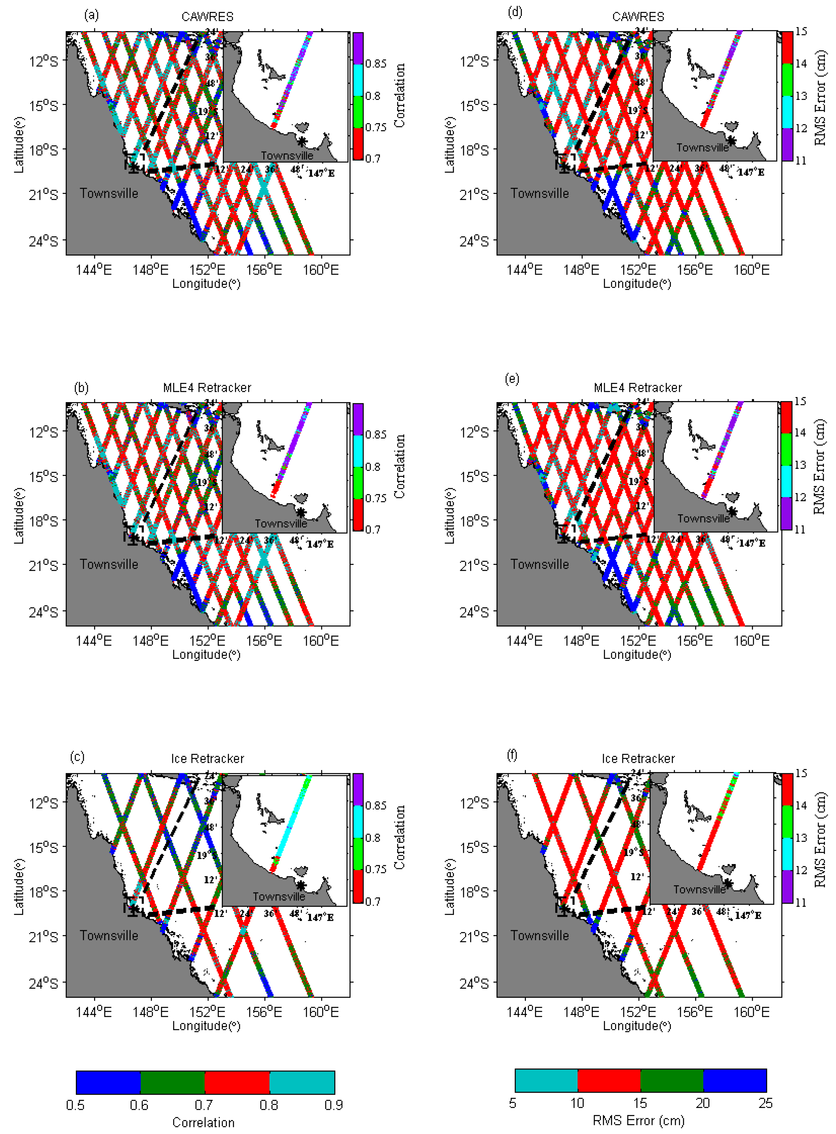
The results over the tested regions emphasise that the retracked sea levels from the CAWRES are consistent with those of the geoid height and tide gauges. It reduces the STD of the MLE4 retracked sea levels by up to 63 cm for Jason-1 and 100 cm for Jason-2. It recovers up to 16% more data than the MLE4 retrackers over the region. Although CAWRES improves the retracking solution over the region, sometimes, the quality of the retrieved SLAs is poor. Therefore, the CAWRES products should be used with caution. Analysis with tide gauges indicates that SLAs from the CAWRES are more reliable than those of from the SGDR products, in the sense that it has a higher (≥0.77) temporal correlation and smaller (≤19 cm) RMS errors. These values indicate that the CAWRES produces more precise and accurate SLAs than those of other retrackers.

The results demonstrated that the CAWRES has the potential of being applied to coastal regions elsewhere, as well as other satellite altimeter waveforms. However, this requires extensive validation activities with various sources of in situ datasets such as high frequency radar and Argo floats. The experimental region has also to be extended to other locations to quantify the performance of CAWRES over different coastal characteristics.

It is expected that the long-term SLA time series can be extended near the coast through retracking waveforms using the CAWRES once new and near future radar altimetry missions start to offer better observation coverage in the coastal zone. However, further development of the coastal waveform retracking method is still required because the current retracking algorithms cannot recover the highly corrupted waveforms when the ground track is much closer to the coastline than what was achieved so far. Further work is needed on the improvement of the existing retracking models by including the effect of land on the altimeter waveforms, or the development of new models by including the scattering from non-linear surfaces to better fit the corrupted waveforms near coasts. In addition, further analysis on the assessment of the offset between various retrackers is needed. This study identified that the offset between the retrackers varies depending on the variation of SWH. Further research is essential regarding the use of the neural network for reducing the offset in the retracked SLAs. The results also show that the error in the SSHs with respect to geoid can reach decade centimetres, which may be due to the existence of the offset value between modthreshold30 and modthreshold20 (modthreshold10) retrackers. Future research should consider the value of offset between those retrackers to improve the accuracy of SSHs.

Studies are currently in progress to examine the applicability of the CAWRES to the other satellite altimeter waveforms, particularly the Sentinel-2 that is equipped with advanced technology of altimetry. In addition, comparison of results with other independent in situ data such as the coastal high frequency radar and Regional Ocean Modelling System is also under further validation.

References

1. Brown, G.S. The average impulse response of a rough surface and its applications. IEEE Trans. Antennas Propag. 1977, 25, 67–74. [Google Scholar] [CrossRef]
2. Deng, X.; Featherstone, W.E. Estimation of contamination of ERS-2 and POSEIDON satellite radar altimetry close to the coasts of Australia. Mar. Geod. 2002, 25, 249–271. [Google Scholar] [CrossRef]
3. Scozzari, A.; Gomez-Enri, J.; Vignudelli, S.; Soldovieri, F. Understanding target-like signals in coastal altimetry: Experimentation of a tomographic imaging technique. Geophys. Res. Lett. 2012, 39, L02602. [Google Scholar] [CrossRef]
4. Amarouche, L.; Thibaut, P.; Zanife, O.Z.; Dumont, J.P.; Vincent, P.; Steunou, N. Improving the Jason-1 ground retracking to better account for attitude effects. Mar. Geod. 2004, 27, 171–197. [Google Scholar] [CrossRef]
5. Deng, X.; Featherstone, W.E. A coastal retracking system for satellite radar altimeter waveforms: Application to ERS-2 around Australia. J. Geophys. Res. 2006, 111, C06012. [Google Scholar] [CrossRef]
6. Fenoglio-Marc, L.; Fehlau, M.; Ferri, L.; Gao, Y.; Vignudelli, S.; Becker, M. Coastal sea surface heights from improved altimeter data in the Mediterranean coastline. In Proceedings of the International Geoscience and Remote Sensing Symposium (IGARSS), Boston, MA, USA, 7–11 July 2008; pp. III423–III426. [Google Scholar]
7. Guo, J.Y.; Gao, Y.G.; Hwang, C.W.; Sun, J.L. A multi-subwaveform parametric retracker of the radar satellite altimetric waveform and recovery of gravity anomalies over coastal oceans. Sci. China Earth Sci. 2010, 53, 610–616. [Google Scholar] [CrossRef]
8. Idris, N.H.; Deng, X. The retracking technique on multi-peak and quasi-specular waveforms for Jason-1 and Jason-2 missions near the coast. Mar. Geod. 2012, 35, 1–21. [Google Scholar] [CrossRef]
9. Quartly, G. Hyperbolic retracker: Removing bright target artifacts from altimetric waveform data. In Proceedings of the ESA Living Planet Symposium, Bergen, Norway, 28 June–2 July 2010. [Google Scholar]
10. Thibaut, P.; Severini, J.; Mailhes, C.; Tourneret, J.Y.; Bronner, E.; Picot, N. A multi-peak model for peaky altimetric waveforms. In Proceedings of the 4th Coastal Altimetry Workshop, Porto, Portugal, 14–15 October 2010. [Google Scholar]
11. Yang, L.; Lin, M.; Liu, Q.; Pan, D. A coastal altimetry retracking strategy based on waveform classification and sub-waveform extraction. Int. J. Remote Sens. 2012, 33, 7806–7819. [Google Scholar] [CrossRef]
12. Vignudelli, S.; Kostianoy, A.G.; Cipollini, P.; Benveniste, J. Coastal Altimetry; Springer: Berlin/Heidelberg, Germany, 2011. [Google Scholar]
13. Gommenginger, C.; Thibaut, P.; Fenoglio-Marc, L.; Quartly, G.; Deng, X.; Gomez-Enri, J.; Challenor, P.; Gao, Y. Retracking altimeter waveforms near the coasts. A review of retracking methods and some applications to coastal waveforms. In Coastal Altimetry; Vignudelli, S., Kostianoy, A.G., Cipollini, P., Benveniste, J., Eds.; Springer: Berlin/Heidelberg, Germany, 2011. [Google Scholar]
14. Andersen, O.B.; Scharroo, R. Range and geophysical corrections in coastal regions: And implications for mean sea surface determination. In Coastal Altimetry; Vignudelli, S., Kostianoy, A.G., Cipollini, P., Benveniste, J., Eds.; Springer: Berlin/Heidelberg, Germany, 2011. [Google Scholar] [CrossRef]
15. Bao, L.; Lu, Y.; Wang, Y. Improved retracking algorithm for oceanic altimeter waveforms. Prog. Nat. Sci. 2009, 19, 195–203. [Google Scholar] [CrossRef]
16. Freeman, J.; Berry, P.A.M. A new approach to retracking ocean and coastal zone multi-mission altimetry. In Proceedings of the 15 Years of Progress in Radar Altimetry, Venice, Italy, 13–18 March 2006. [Google Scholar]
17. Idris, N.H.; Deng, X.; Andersen, O.B. The importance of coastal altimetry retracking and detiding: A case study around the Great Barrier Reef, Australia. Int. J. Remote Sens. 2014, 35, 1729–1740. [Google Scholar] [CrossRef]
18. Lee, H.; Shum, C.K.; Yi, Y.; Braun, A.; Kuo, C.Y. Laurentia crustal motion observed using TOPEX/POSEIDON radar altimetry over land. J. Geodyn. 2008, 46, 182–193. [Google Scholar] [CrossRef]
19. Passaro, M.; Cipollini, P.; Vignudelli, S.; Quartly, G.D.; Snaith, H.M. ALES: A multi-mission adaptive subwaveform retracker for coastal and open ocean altimetry. Remote Sens. Environ. 2014, 145, 173–189. [Google Scholar] [CrossRef]
20. Thibaut, P.; Poission, J.C.; Halimi, A.; Mailhes, C.; Tourneret, J.Y.; Boy, F.; Picot, N. A review of CLS retracking solutions for coastal altimeter workshop. In Proceedings of the 5th Coastal Altimetry Workshop, San Diego, CA, USA, 16–18 October 2011. [Google Scholar]
21. Idris, N.H.; Xiaoli, D.; Idris, N.H. Comparison of retracked coastal altimetry sea levels against high frequency radar on the continental shelf of the Great Barrier Reef, Australia. J. Appl. Remote Sens. 2017, 11. [Google Scholar] [CrossRef]
22. Anzenhoufer, M.; Shum, C.K.; Renstch, M. Coastal Altimetry and Applications; The Ohio State University: Columbus, OH, USA, 1999; p. 36. [Google Scholar]
23. Berry, P.A.M.; Bracke, H.; Jasper, A. Retracking ERS-1 altimeter waveforms over land for topographic height determination: An expert systems approach. In Proceedings of the 3rd ERS Symposium on Space at the Service of our Environment, Florence, Italy, 14–21 March 1997; p. 403. [Google Scholar]
24. Roesler, C.J.; Emery, W.; Kim, S. Evaluating the use of high-frequency radar coastal currents to correct satellite altimetry. J. Geophys. Res. Oceans 2013, 118, 3240–3259. [Google Scholar] [CrossRef]
25. Deng, X. Improvement of Geodetic Parameter Estimation in Coastal Regions from Satellite Radar Altimetry; Curtin University of Technology: Bentley, Australia, 2003. [Google Scholar]
26. Quartly, G.; Cipollini, P. Seamless transition from ocean to coastal retracking algorithms. In Proceedings of the OSTST Meeting, Venice, Italy, 27–29 September 2012. [Google Scholar]
27. Pavlis, N.K.; Holmes, S.A. A preliminary gravitational model to degree 2160. In Proceedings of the IAG International Symposium on Gravity, Geoid and Space Missions, Porto, Portugal, 30 August–3 September 2004. [Google Scholar]
28. Andersen, O.B.; Knudsen, P. The DTU10 mean sea surface and mean dynamic topography. Improvements in the Artic and coastal zone. In Proceedings of the OSTST Meeting, Lisbon, Portugal, 18–20 October 2010. [Google Scholar]
29. Albertos, P.; Sala, A.; Olivares, M. Fuzzy logic controllers. Advantages and drawbacks. In Proceedings of the VIII Congreso Latinoamericano de Control Automático IFAC, Viña del Mar, Chile, 14 September 1998; pp. 833–844. [Google Scholar]
30. Idris, N.H.; Deng, X. An iterative coastal altimetry retracking strategy based on fuzzy expert system for improving sea surface height estimates. In Proceedings of the 2013 IEEE International Geoscience and Remote Sensing Symposium-IGARSS, Melbourne, Australia, 21–26 July 2013; pp. 2954–2957. [Google Scholar]
31. Andersen, O.B. Shallow water tides in the northwest European shelf region from Topex/Poseidon altimetry. J. Geophys. Res. Oceans 1999, 104, 7729–7741. [Google Scholar] [CrossRef]
32. Fairhead, J.D.; Green, C.M.; Odegard, M.E. Satellite-derived gravity having an impact on marine exploration. Lead. Edge 2001, 20, 873–876. [Google Scholar] [CrossRef]
33. Martin, T.V.; Zwally, H.J.; Brenner, A.C.; Bindschadler, R.A. Analysis and Retracking of Continental Ice Sheet Radar Altimeter Waveforms. J. Geophys. Res. 1983, 88, 1608–1616. [Google Scholar] [CrossRef]
34. Hayne, G. Radar altimeter mean return waveforms from near-normal-incidence ocean surface scattering. IEEE Trans. Antennas Propag. 1980, 28, 687–692. [Google Scholar] [CrossRef]
35. Abbasi, B. A neural network applied to estimate process capability of non-normal processes. Experts Syst. Appl. 2009, 36, 3093–3100. [Google Scholar] [CrossRef]
36. Beale, M.H.; Hagan, M.T.; Demuth, H.B. Neural Network Toolbox: User’s Guide; The MathWorks: Natick, MA, USA, 2013. [Google Scholar]
37. Sovan, L.; Guegan, F.F. Artificial neural networks as a tool in ecological modelling, an introduction. Ecol. Model. 1999, 120, 65–73. [Google Scholar]
38. Emery, W.; Thomson, R.E. Data Analysis Methods in Physical Oceanography; Elsevier: Sydney, Australia, 2004. [Google Scholar]
39. Hwang, C.; Guo, J.; Deng, X.; Hsu, H.Y.; Liu, Y. Gravity anomalies in coastal waters from retracked Geosat/GM altimetry: Comparison with shipborne and airborne gravity data. J. Geod. 2006, 80, 204–216. [Google Scholar] [CrossRef]
40. Nahavandchi, H. Two different methods of geoidal height determination using a spherical harmonic representation of the geopotential, topographic corrections and the height anomaly-geoidal height difference. J. Geod. 2002, 76, 345–352. [Google Scholar] [CrossRef]
41. AVISO. Coastal and Hydrology Altimetry Product (PISTACH) Handbook, 1st ed.; Centre National d’Études Spatiales (CNES): Paris, France, 2010; p. 58.
Figure 1. Jason-1 (dash line) and Jason-2/OSTM (solid line) satellite passes in the Great Barrier Reef, Australia. The red stars show the tide gauge stations.
Remotesensing 09 00603 g001
Figure 2. Block diagram of the CAWRES, consisting of four major parts: neural network, waveform classification, waveform retracking and fuzzy expert system.
Remotesensing 09 00603 g002
Figure 3. (Top panel) The fuzzy set of the goodness of fit (r2) consists of two fuzzy sets: poor (in magenta) and good (in yellow). The r2 of 0.82 is a member of the poor set with a degree of membership of 0.03, and at the same time, it is also a member of the good set with a degree of 0.1. (Bottom panel) The fuzzy set of the differences between two successive retracked SLAs (Dif_ssh_prev1) consists of two fuzzy sets: small (in cyan) and large (in blue).
Remotesensing 09 00603 g003
Figure 4. The retracked SLA profiles (top) and their ranking values (bottom) during a few iterations. An arbitrary constant of 5 and 10 was added to the second and third iterations, respectively, for visual clarity. Red circles (top panel) show problematic areas where ‘low ranking’ retracked SLAs are found.
Remotesensing 09 00603 g004
Figure 5. Implementation of the MLF neural network for offset reduction during the training (top panel) and prediction (bottom panel) modes. In the training mode, the training samples of sub-waveform (or full-waveform) and modthreshold30 retracked SLAs are supplied to the input and output layers, respectively, to optimise the weight coefficients. In the prediction mode, the new set of sub-waveforms (or full-waveform) retracked SLAs are supplied to the input layer to predict the modthreshold30 retracked SLAs in the output layer based on the optimised weights obtained from the training mode. The predicted modthreshold30 retracked SLAs correspond to the realigned/unbiased sub-waveform (or full-waveform) retracked SLAs.
Remotesensing 09 00603 g005
Figure 6. Spatial plots of the temporal correlation and RMS error of sea level anomaly along Jason-2 pass 175 from different retracking methods with respect to Townsville tide gauge station.
Remotesensing 09 00603 g006
Figure 7. Jason-2 retracked SLAs before and after the offset reductions using the MLF neural network and the mean method along pass (a) 214 from cycle 50, and (b) 175 from cycle 40. The box indicates the area where retracking algorithms are switched. No arbitrary constant is added to the SLA profiles (reprinted from [30]).
Remotesensing 09 00603 g007
Figure 8. Sea level anomaly profiles of Jason-2 altimetry along (a) pass 175 from cycle 80, (b) pass 214 from cycle 100, and (c) pass 149 from cycle 120. An arbitrary constant of −2 m, −1 m, 1 m, and 2 m was added to MLE4, Oce3, Ice3 and Red3 retracked SLAs, respectively, for visual clarity. No constant value was added to Ice1 and CAWRES retracked SLAs.
Remotesensing 09 00603 g008
Figure 9. Spatial plots of the temporal correlation (ac) and RMS error (df) of SLAs from different retracking methods with respect to the Townsville tide gauge station.
Remotesensing 09 00603 g009