
2D Normalized Iterative Hard Thresholding Algorithm for Fast Compressive Radar Imaging
by
 , ,
, ,
Gongxin Li
1,2 ,
,
Jia Yang
1,2,
Wenguang Yang
1,2,
Yuechao Wang
1,
Wenxue Wang
1,* and
Lianqing Liu
1,* 1
State Key Laboratory of Robotics, Shenyang Institute of Automation Chinese Academy of Sciences, Shenyang 110016, China
2
University of the Chinese Academy of Sciences, Beijing 100049, China
*
Authors to whom correspondence should be addressed.
Remote Sens. 2017, 9(6), 619; https://doi.org/10.3390/rs9060619
Submission received: 18 March 2017
/
Revised: 9 June 2017
/
Accepted: 13 June 2017
/
Published: 16 June 2017
(This article belongs to the Special Issue Radar Systems for the Societal Challenges)
Abstract
:Compressive radar imaging has attracted considerable attention because it substantially reduces imaging time through directly compressive sampling. However, a problem that must be addressed for compressive radar imaging systems is the high computational complexity of reconstruction of sparse signals. In this paper, a novel algorithm, called two-dimensional (2D) normalized iterative hard thresholding (NIHT) or 2D-NIHT algorithm, is proposed to directly reconstruct radar images in the matrix domain. The reconstruction performance of 2D-NIHT algorithm was validated by an experiment on recovering a synthetic 2D sparse signal, and the superiority of the 2D-NIHT algorithm to the NIHT algorithm was demonstrated by a comprehensive comparison of its reconstruction performance. Moreover, to be used in compressive radar imaging systems, a 2D sampling model was also proposed to compress the range and azimuth data simultaneously. The practical application of the 2D-NIHT algorithm in radar systems was validated by recovering two radar scenes with noise at different signal-to-noise ratios, and the results showed that the 2D-NIHT algorithm could reconstruct radar scenes with a high probability of exact recovery in the matrix domain. In addition, the reconstruction performance of the 2D-NIHT algorithm was compared with four existing efficient reconstruction algorithms using the two radar scenes, and the results illustrated that, compared to the other algorithms, the 2D-NIHT algorithm could dramatically reduce the computational complexity in signal reconstruction and successfully reconstruct 2D sparse images with a high probability of exact recovery.

1. Introduction
Radar, an object detection system using radio waves to detect objects and determine their spatial positions, has been applied in many fields, including radar astronomy, geographical environment surveillance system, and air defense systems. The demand of radar systems for high-resolution and high-speed imaging capabilities is increasing and results in a strong desire for higher bandwidths and more sampling time, which places significant pressure on radar hardware equipment and imaging costs. However, classical time–frequency uncertainty principles based on the Shannon sampling theorem have limited the development of high-resolution and high–speed radar imaging [1]. Compressive sensing, as an effective approach for direct compressive sampling, has great potential application for radar imaging and is able to solve the problems that radar systems currently face, that is, the mass time requirement of signal sampling and reconstruction for high–resolution imaging [2]. Meanwhile, a compressive imaging method can simplify the structure of a radar system, allowing elimination of the matched filter for pulse compression at the receiver and thereby reducing the need for analog-to-digital convertors [3,4,5,6].
Some achievements of radar imaging based on the compressive sensing principle have been reported [1,3,7,8]. Braniuk and co-workers first applied the compressive sensing theorem in radar imaging systems and confirmed the feasibility of compressive radar imaging by theoretical analysis and numerical experiments [3]. Zhang and co-workers proposed a framework to realize high–resolution inverse synthetic aperture radar (ISAR) imaging with limited measured data based on the theory of compressed sampling [4]. Ender presented generic system architectures and implementation considerations to address some further steps to compressive radar imaging and applied the compressive sensing in pulse compression, radar imaging and air space surveillance with array antennas [9]. An approach that employed pulse accumulation and weighted compressive sensing was also proposed by Zhang and co-workers under low signal-to-noise ratio (SNR) conditions, to realize high-resolution imaging and reduce sensitivity to noise [10]. Moreover, many reconstruction algorithms of compressive radar images have proposed. For example, Xie and co-workers proposed a smoothed L0 norm (SL0) algorithm to obtain fast radar imaging based on a compressive sensing [11]; Bhattacharya and co-workers used convex optimization through projection onto convex sets or greedy algorithms to decode compressive synthetic aperture radar (SAR) images [12,13]; and Yu and co-workers introduced a turbo-like iterative thresholding algorithm to recover SAR images [14]. The methods of compressive radar imaging based on these reconstruction algorithms can obtain high-resolution radar images with very small amounts of echo data, and improve the radar imaging speed remarkably, compared with conventional radar imaging methods. However, the radar imaging time is still very long, especially for high-resolution radar imaging, because the conventional strategies for 2D signal reconstruction usually involve stacking a matrix of 2D signals into a huge column vector based on the vector space model, and then recovering the huge vector signal with reconstruction algorithms in the 1D domain [15,16]. These approaches exponentially increase the computational complexity involved in recovering 2D sparse signals and the memory requirement for storing the large-bandwidth data of the radar images [17]. In addition, these approaches ignore the intrinsic spatial structure of 2D signals [16], especially the coupled range and azimuth information of radar imaging.
To address these drawbacks, some 2D reconstruction algorithms that directly leverage the matrix structure of 2D sparse signals have been proposed recently [16,17,18,19,20,21], and some have been used in radar imaging systems. For example, a fast reconstruction algorithm, called two-dimensional smoothed L0 norm (2D-SL0) algorithm, has been proposed to reduce computational complexity and economize on the memory required by directly utilizes the matrix structure to recover the 2D sparse signals and is designed [20], but the reconstruction quality of the natural image is poor. Another novel algorithm called the 2D orthogonal matching pursuit (2D-OMP) algorithm, which was extended from 1D-OMP, has been developed to reconstruct 2D sparse signals [17]. In this algorithm, each atom in the dictionary is a matrix. At each iteration, the best matched matrix atom is selected by projecting the sample matrix onto 2D atoms and the weights for the selected atoms are then updated via the least square. This algorithm significantly reduces the computational complexity with a matrix structure, but it still requires a great deal of memory usage and is suitable only for the square matrix of 2D sparse signals. In addition, an iterative gradient projection algorithm for 2D sparse image reconstruction has been proposed, in which the sparse solution is searched iteratively from the 2D solution space and then updated by gradient descent of the total variation. It recovers the natural image perfectly, being conducive to reduction in both computational complexity and memory requirements for the measurement matrix [18]; however, the algorithm suffers from the limitation that the sparse signals must be square.
In this paper, we propose a novel reconstruction algorithm of 2D sparse signals, called the 2D normalized iterative hard thresholding (2D-NIHT) algorithm, which is extended from the normalized iterative hard thresholding (NIHT) algorithm [22] to reduce the reconstruction time in radar imaging by recovering radar images in the matrix domain directly, and the effectiveness and superiority of the algorithm are theoretically proved and demonstrated by experiments. Moreover, we also present a 2D compressive sampling model of radar imaging systems, which compresses range and azimuth information simultaneously and also ensures that the 2D-NIHT algorithm can be implemented in a compressive radar imaging system.
This paper is organized as follows. In Section 2, we briefly present the compressive sensing theory and the NIHT algorithm. In Section 3, we introduce the radar imaging model based on compressive sensing. In Section 4, we describe the 2D-NIHT algorithm in detail and prove its convergence. In Section 5, some experiments using randomly synthetic 2D signals and actual radar images are presented. Finally, in Section 6, we draw conclusions.
2. Brief Introduction of Compressive Sensing and the NIHT Algorithm
2.1. Compressive Sensing
The basic theory of compressive sensing is formulated as follows. For a k-sparse signal , which contains no more than k nonzero elements, a measurement matrix , and an observation vector (or measurements) , where , the core problem of compressive sensing is to reconstruct the sparse signal by solving the following linear equation:
which acquires no unique candidate signals for because it is under-determined. However, the signal can be recovered from and through many available reconstruction algorithms, such as, compressive sampling matching pursuit (CoSaMP) [23], iterative hard thresholding (IHT) [24], and Smoothed L0 norm [25,26] algorithms, with high reliability if the measurement matrix satisfies the restricted isometry property (RIP) condition [27] and the signal is sparse enough, that is, [2]. However, if the signals data are huge, these algorithms are inevitably costly in terms of the computational complexity for recovering sparse signals as well as the memory usage for storing the measurement matrices.
2.2. NIHT Algorithm
The NIHT algorithm, extended from the IHT algorithm, was first proposed by Blumensath [22] and has become an effective method to calculate near-optimal solutions. The algorithm solves the problem of Equation (1) using the following optimization problem:
where denotes the -norm, counts the nonzero elements, and is the penalty factor. The algorithm is described as follows.
Let ; then,
where is a nonlinear operator that sets all but the maximal elements in absolute terms of to be zero, and is the step size at the nth iteration. In the NIHT algorithm, is adaptively determined using the following procedures.
Let denotes the support set of , and is the negative gradient of evaluated at at the iteration; then, denotes the sub-vector of that contains only the elements in the set of , and is the sub-matrix of that contains corresponding columns indexed by . The adaptive step size and new approximation of are updated as below.
Given the approximation of at the iteration and its support set , the adaptive step size is calculated by the following equation:
and the new proposition is obtained from by the following equation:
If the support set of is equal to that of , namely, , then .
However, if , the step size obtained in Equation (4) cannot guarantee that the Equation (2) has a maximal reduction, and the approximation of converges. In this case, the sufficient condition for the algorithm to guarantee convergent approximation of is that , where
and is a small constant. Therefore, in the case that , it is necessary to calculate and check whether . If this holds, then and . Otherwise, the step size must be shrunk; in [22], it is proposed to shrink the step size by updating , where . A new proposition is then calculated based on the shrunken step size , and a new is obtained for rechecking whether . These procedures are repeated until , and then and .
The NIHT algorithm is a modification of the IHT algorithm by the introduction of a simple adaptive step size and line search, which not only makes the algorithm performance independent of arbitrary scaling of but also guarantees its convergence regardless of whether the theoretical conditions for IHT are satisfied. Furthermore, the NIHT algorithm is faster than many other state-of-the-art approaches that show similar empirical performance, such as the norm algorithm and OMP algorithm [22].
3. Radar Imaging Model Based on Compressive Sensing
3.1. 2D Compressive Sensing
For a 2D K-sparse signal , a measurement matrix pair and , and an observation matrix , the 2D compressive sensing model is formulated as follows:
where is the transpose of , , and . The sparsity of the 2D signal is defined as , in which denotes the column vector of the matrix , means that the 2D signal has no more than nonzero elements.
One-dimensional compressive sensing can be treated as a special form of 2D compressive sensing in the case that . And the 2D compressive sensing model is also equivalent to the 1D compressive sensing model by the following operations:
where ‘’ denotes the operation of the Kronecker product and denotes the vectorization of a matrix by stacking the columns of the matrix into a single column vector. Therefore, some properties of 1D compressive sensing are also suitable for 2D compressive sensing.
3.2. Compressive Radar Imaging Model
For a typical stepped frequency radar, the echo data of the () aspect angle and () sampling frequency point can be described as:
where denotes the scattering intensity of the discrete position, is the number of aspect angles and denotes the number of sub-pulse in a burst [21].
Suppose and , and let and denote matrix of echo data and scattering intensity of the discrete position, respectively. and represent the discrete Fourier dictionary of azimuth and range, respectively. Then, a typical radar imaging model can be formulated as follows:
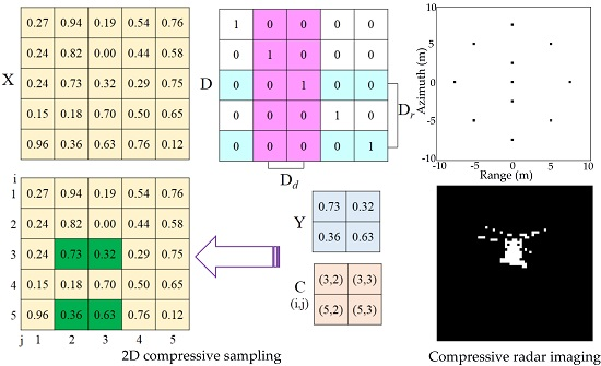
To apply the 2D compressive sensing in a radar imaging system, an effective compressive sampling method should be designed at first for reducing the length of observation signals. Compared with the 1D compressive sampling model by which a small number of either frequency points or aspect angles is randomly sampled [9,28], the 2D compressive sampling method compresses and randomly samples both of frequency points and aspect angles simultaneously. Moreover, in the process of compressive sampling of a radar system, any pixel of a scene has just two states: sampled or un-sampled. So, the sampling matrix is designed specially and each entry of the matrix is either 1 or 0, indicating that the corresponding pixel of the radar imaging scene is sampled or un-sampled, respectively. The 2D compressive sampling method in radar imaging is designed by the following procedures: (i) set a matrix , in which each entry is either 0 () or 1 (); (ii) randomly select rows of to produce a sampling matrix , and columns of to produce a sampling matrix , respectively. The sampling matrix pair and compress the range information from to and azimuth information from to , respectively. In order to more clearly describe the 2D compressive sampling process, a simple example is given, as shown in Figure 1. It is obvious that the sampling process can compress a matrix to a matrix of lower dimensions, and can be also regarded as the set of elements collected from the original scene at the rows and columns, which are determined by the column position of “1” of and , respectively. Moreover, the compressive sampling method is actually feasible, which has been demonstrated by its application in compressive imaging with atomic force microscopy [29] and scanning ion conductance microscopy [30].
Then, the 2D compressive radar imaging model is formulated as follows:
The 2D compressive radar imaging model has the capability of dramatically reducing the sampled pixels of a radar scene from dimensions to dimensions and reconstructing the scene in matrix domain with much less reconstruction time using the 2D-NIHT algorithm presented as below.
4. 2D-NIHT Algorithm
4.1. Description of the 2D-NIHT Algorithm
In this study, inspired by the conventional NIHT algorithm, a 2D-NIHT algorithm is proposed to recover 2D sparse signals based on the 2D compressive sensing model, as described in the Equation (7), by solving the following optimization problem:
where denotes the Frobenius norm of a matrix, that is, .
The above optimization problem can be solved by the following iterative procedures:
where is the nonlinear operation that sets all elements of matrix as zero except for the maximum elements of in absolute terms.
At the iteration, denotes the support matrix of , in which and are the entries of the matrices and at the row and the column, respectively, and is the signum function. is the negative gradient matrix of evaluated at . Then, denotes the matrix derived from by setting if , in which the “” is the element-wise multiplication, and . Similar to the arguments in [22], the step size is calculated by the following equation:
Hence, a new proposition is calculated by the following equation:
Next, it is necessary to determine whether the new proposition is an approximation solution to the problem in Equation (12) at the iteration by comparing the support matrices and described as follows.
If is equal to , then ; otherwise, the sufficient condition must be satisfied to guarantee the convergence of the approximation solution of , that is, , where:
and is a small constant. If , then the step size must be shrunk by updating with a constant , and a new proposition is calculated based on the shrunk step size by Equation (15). The new is accordingly obtained for rechecking whether . These procedures are repeated until , and then and .
The implementation of the 2D-NIHT algorithm is listed in Algorithm 1.
In general, compared with NIHT method, which places a great demand on memory space for measurement matrix storage, the 2D-NIHT algorithm realizes 2D sparse signal recovery in matrix domain with far less storage space requirement. The 2D-NIHT algorithm requires memory units to store the measurement matrices; in contrast, the measurement matrix of NIHT algorithm requires memory units. The 2D-NIHT algorithm immensely reduces the storage space requirement for the measurement matrix, which is valuable in practice, especially for portable radar systems.
| Algorithm 1. 2D normalized iterative hard thresholding algorithm. |
| Input: , , , . |
| Initialize: , . |
| Iterate for , until the stopping criterion is met: |
| Step 1. ; |
| Step 2. ; |
| Step 3. ; |
| Step 4. ; |
| Step 5. If is equal to , then go to Step 6; otherwise |
| set , |
| and repeat the following procedures until : |
| , , |
| ; |
| Step 6. ; |
| Step 7. ; |
| Step 8. . |
| Output: . |
4.2. Convergence of the 2D-NIHT Algorithm
The sufficient condition for the convergence the 2D-NIHT algorithm is given in the following convergence theorem.
Theorem 1.
Given a 2D compressive sensing model , where is a 2D K-sparse signal and is the best K-term approximation of the signal , if the matrix satisfies the RIP condition for any 2K-sparse signal :
where and are two constants, then the 2D-NIHT algorithm can recover by an approximation at the iteration, satisfying:
where is the observation error.
Furthermore, after no more than:
Iterations, the 2D-NIHT algorithm recovers with an accuracy of:
where:
Theorem 1 (proof shown in Appendix A) indicates that the 2D-NIHT algorithm can find an optimal solution that approximates the true signal with finite iterations, and the approximation is bounded by , which includes two parts: one is determined by the observation error and the other is determined by the deviation between the signal and the best -term approximation. Assuming that the observation error is zero and is -sparse, the algorithm can recover exactly. For practical radar imaging, the reconstruction error is naturally bounded by the observation error.
5. Results
In this section, on the one hand, an experiment with syncretic sparse images was conducted to demonstrate the feasibility of the 2D-NIHT algorithm and its superiority to the NIHT algorithm in reconstruction time. On the other hand, two SAR scenes were used to exam the reconstruction performance of the 2D-NIHT algorithm under different SNR levels and its superiority to other five efficient reconstruction algorithms of sparse signals in compressive radar imaging systems. All data were analyzed in the Matlab R2013a environment using an Intel Core 4, 3.20 GHz processor with 4.0 GB of memory under the Microsoft Windows 7 operating system. The reconstruction time, which is the CPU time, was utilized as an indicator of the computational complexity of signals reconstruction. The probability of exact recovery, which is a crucial criterion for evaluating the practicability of the algorithm, was calculated by the equation , where , and were original signals and the recovered signals, respectively.
5.1. Experiments on Synthetic Images
5.1.1. Efficiency of the 2D-NIHT Algorithm in 2D Signal Reconstruction
In this experiment, a randomly synthetic 2D sparse signal of with size of and a sparsity of 200, as shown in Figure 2a, was used to validate the efficiency of the 2D-NIHT algorithm. The observation matrix was acquired by the model with the compressive sampling rate of 0.5 in both row and column, and then the recovered signal was reconstructed using the 2D-NIHT algorithm from . As shown in Figure 2b, it was obvious that the algorithm perfectly recovered the synthetic 2D sparse signal without any information loss. And, as shown in Figure 2c, it took a finite number of iterations, which was even far less than the sparsity of the signal. Moreover, only 0.25 s was spent on the whole process of the sparse signal recovery.
5.1.2. Comparison with the NIHT Algorithm
To demonstrate the superiority of the 2D-NIHT algorithm to the NIHT algorithm, a series of synthetic images were used to test their reconstruction performances. The reconstruction performances of the 2D-NIHT and the NIHT algorithms were comprehensively compared by varying the sparsities and lengths of measurements, respectively.
To test the reconstruction performance of the two algorithms under various sparsities, some randomly synthetic 2D sparse signals with different sparsities were used as testing images, and the measurements of a fixed length were acquired with a constant compressive sampling rates of 0.5 for both rows and columns. To test the reconstruction performance of the NIHT algorithm, the 2D signals were also vectorized by firstly and the measurements were acquired based on Equation (1) with a constant compressive sampling rate of 0.25 for any signal . The reconstruction performances of the two algorithms, as shown in Figure 3a, demonstrated that, on one hand, both algorithms could obtain the probability of exact recovery of 1 with a smaller sparsity (≤550), and then their probabilities of exact recovery of both algorithms decreased as the sparsity increased; on the other hand, the reconstruction time of the 2D-NIHT algorithm was far less than that of the NIHT algorithm, and the difference of recovery time between the two algorithms became larger with an increase in the signal sparsity.
To test the reconstruction performance of the two algorithms with measurements of various lengths, 2D sparse signals with a fixed sparsity of were generated for testing and the measurements were obtained with different lengths. For the sparse signal , the lengths of the measurement for the 2D-NIHT algorithm were set as and the lengths of measurement for NIHT algorithm was set as accordingly. The reconstruction performances of the two algorithms, as shown in Figure 3b, indicated that both algorithms could acquire a very high probability of exact recovery with measurements of large size (>40 × 40), while the reconstruction time of the NIHT algorithm was far greater than that of the 2D-NIHT algorithm.
Overall, the 2D-NIHT algorithm and the NIHT algorithm displayed a similar tendency in the probability of exact recovery with respect to the sparsity of signals and the size of measurements, indicating that they had consistent performances in the reconstruction convergence and accuracy, and the reconstruction time of the 2D-NIHT algorithm was much less than that of the NIHT algorithm, illustrating that the proposed 2D-NIHT algorithm dramatically reduced computational complexity in signal reconstruction.
5.2. Experiments on Actual Radar Images
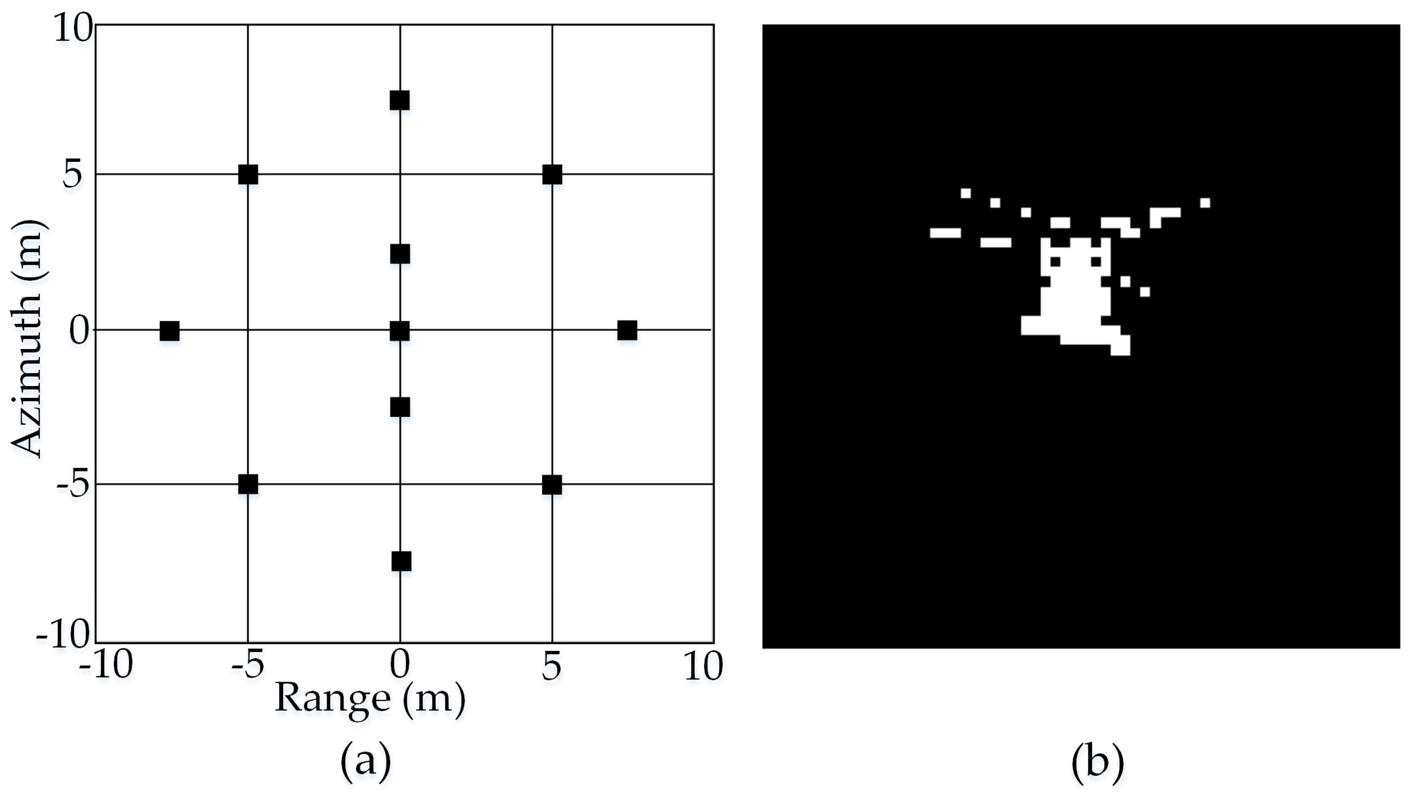
In this section, two SAR scenes were used to verify the efficiency and superiority of the 2D-NIHT algorithm in compressive radar imaging systems, as shown in Figure 4. One was a simple scene that acquired 11 point targets (Figure 4a), and the other was a helicopter acquired by a SAR (Figure 4b). The SAR parameters were set such that the carrier frequency was 2 GHz, the working frequency was 9.5 GHz–10.5 GHz with a step size 20 MHz, the sampling number was , the observation azimuth varied within −3.2°~3.0°, and corresponding sampling number was . In addition, it was unavoidable that there were noises in the actual radar imaging system, so, the noises of different SNR levels were also added in the echo signals to explore the influence of the noise on the reconstruction performance of the 2D-NIHT algorithm.
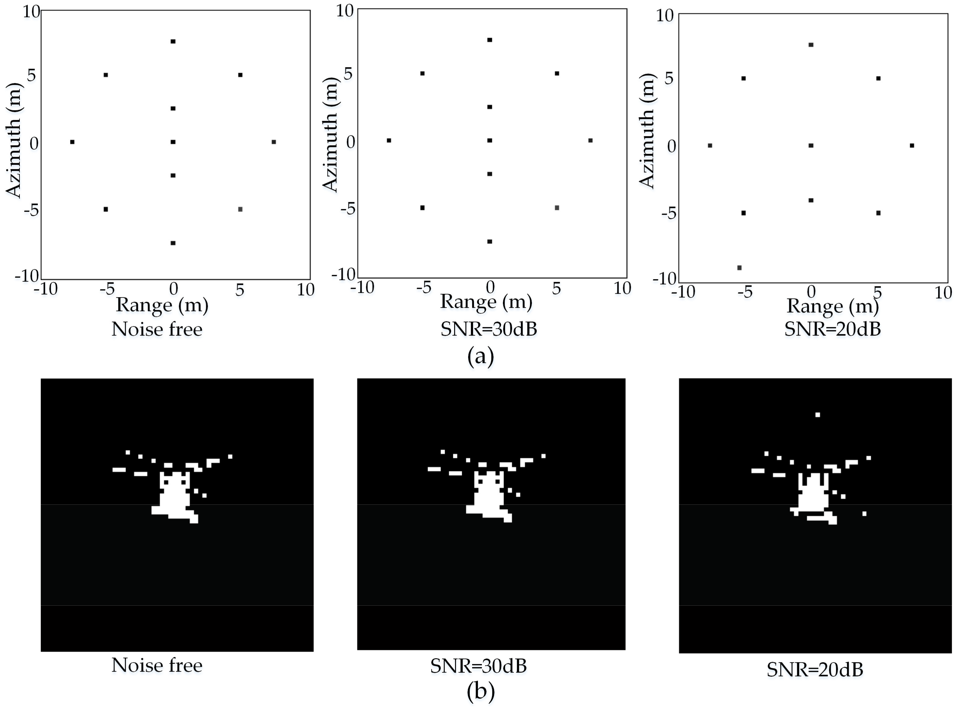
To test radar imaging performance using the 2D-NIHT algorithm in the presence of noise, Gaussian white noises with different SNR levels (noise free, 30 dB and 20 dB) were added into the echo signals. Figure 5 shows the imaging results of the 11 point targets (Figure 5a) and the helicopter (Figure 5b) with different SNR levels of noises using the 2D-NIHT algorithm. The compressive sampling rates were 0.5 in the range and azimuth information for the two SAR scenes. The imaging results illustrated that the actual target positions and amplitudes of the both scenes were reconstructed without any information loss at the higher SNR level (noise free and 30 dB). At the low SNR level (20 dB), the imaging results contained some false values at the target positions for both scenes. Moreover, it was obvious that the reconstructed image using the 2D-NIHT algorithm was clean without any noise, because the nonlinear operation process of in the 2D-NIHT algorithm was capable of setting elements of as 0 and these elements contained most of the noises. Therefore, the 2D-NIHT algorithm is an effective method to remove background noise used in compressive radar imaging systems.
In addition, four other algorithms, including CoSaMP, SL0, block-based compressive sensing (BCS) [31], and NIHT algorithms, were used to recover the two scenes without noises, and their reconstruction performances were compared with the 2D-NIHT algorithms in terms of reconstruction time and probability of exact recovery. The simulation for each SAR scene was repeated 20 times with every algorithm, and the statistical average values and standard deviations in reconstruction time and probability of exact recovery for the five algorithms were achieved, as shown in Table 1. The results demonstrate that, compared with the other four algorithms, the 2D-NIHT algorithm could acquire the reconstructed images with ultrahigh probability of exact recovery, and its performance in reconstruction time was only a little inferior to the BCS model, which, however, had the worst performance for the probability of exact recovery. Therefore, the 2D-NIHT is capable of significantly reducing the computational complexity and reconstruction time for recovering radar images and has an overall performance superior to the other four algorithms.
6. Conclusions
In this paper, a 2D-NIHT algorithm was proposed to solve the problem that compressive radar imaging systems confront, that is, the high computational complexity involved in recovering sparse signals. The algorithm recovered 2D sparse signals by directly leveraging the matrix structure of the signals with robust and ultra-high probability, as proved theoretically and demonstrated by experiments. The number of iterations of the 2D-NIHT algorithm in signal reconstruction is far fewer than the sparsity of the testing signals, and reconstruction time of the 2D-NIHT algorithm is far less than that of the NIHT algorithm, indicating that the 2D-NIHT algorithm dramatically reduces the computational complexity and reconstruction time compared with the NIHT algorithm. Particularly, the radar scenes can be also recovered successfully by the 2D-NIHT algorithm with high reconstruction performance, and the 2D-NIHT algorithm also displays significant superiority in overall reconstruction performance in radar imaging system to other four algorithms. Moreover, the 2D-NIHT algorithm offers great potential for general application of compressive sensing in electromagnetics and remote sensing to realize fast imaging.
Acknowledgments
This work was supported by the National Natural Science Foundation of China (Grant No. 61327014, Grant No. 61433017) and the CAS/SAFEA International Partnership Program for Creative Research Teams.
Author Contributions
Gongxin Li and Wenxue Wang conceived and designed the research; Gongxin Li and Jia Yang performed the experiments; Gongxin Li, Wenxue Wang and Lianqing Liu analyzed the data; Gongxin Li, Wenxue Wang and Lianqing Liu wrote the paper.
Conflicts of Interest
The authors declare no conflict of interest. The founding sponsors had no role in the design of the study; in the collection, analyses, or interpretation of data; in the writing of the manuscript, and in the decision to publish the results.
Appendix A
If the measurement matrix satisfies the RIP condition in the 1D compressive sensing model (1), then the following lemma holds, which have been proved in [23].
Lemma A1.
Suppose that the matrix satisfies the RIP with a restricted isometry constant and an index set such that , then, for any K-sparse signal , the following inequality holds
There is also a relation between the Frobenius norm and the Euclidean norm in the Kronecker product of matrices, stated as in the following Lemma.
Lemma A2.
For any matrices , , and , there exists the following equivalence relationship between the Frobenius norm and the Euclidean norm:
The following notions will also be used in our proof.
Suppose is the best K-term approximation of the K-sparse signal ; then,
Then, the proof of Theorem 1 is described as follows.
Proof.
As described in Equation (8), the 2D compressive sensing model is equivalent to the 1D compressive sensing model, which means that many properties of the 2D compressive sensing are similar to those of the 1D compressive sensing. Therefore, the proof method of convergence of the NIHT algorithm can be also applied to that of the 2D-NIHT algorithm. In this proof, at first, the convergence model of the 2D-NIHT algorithm should be transformed from 2D to 1D; then, we will use some similar results of [22] to get the convergence properties of the 2D-NIHT algorithm.
Firstly, the convergence model is transformed from 2D to 1D, as described below:
Suppose that the support matrix of the error belongs to the matrix ; namely, the non-zero entries of the support matrix of the error must occur on the corresponding positions of nonzero entries of or . Similar to , it is obvious that there are unique corresponding support matrices and for matrices and , respectively. Because the following is true:
Similar to the proof in [24], we have:
Based on Lemma A2, we then have:
where . and . Then, the inequality (A8) can be rewritten as follows:
Based on Lemma A1, we have:
Secondly, we also use the results similar to [22], namely:
where . Then, (A11) can also be simplified as:
If and [22], we then have:
Equation (A16) can also be rewritten as:
Note that , then by iterative calculation using Equation (A17), we then have:
Finally, we have:
Furthermore, after no more than:
iterations, the 2D-NIHT algorithm recovers with an accuracy of:
where:
References
- Herman, M.A.; Strohmer, T. High-resolution radar via compressed sensing. IEEE Trans. Signal Process. 2009, 57, 2275–2284. [Google Scholar] [CrossRef]
- Baraniuk, R.G. Compressive sensing. IEEE Signal Process. Mag. 2007, 24, 118–124. [Google Scholar] [CrossRef]
- Baraniuk, R.; Steeghs, P. Compressive radar imaging. In Proceedings of the 2007 IEEE Radar Conference, Boston, MA, USA, 17–20 April 2007; pp. 128–133. [Google Scholar]
- Zhang, L.; Xing, M.D.; Qiu, C.W.; Li, J.; Bao, Z. Achieving higher resolution ISAR imaging with limited pulses via compressed sampling. IEEE Geosci. Remote Sens. 2009, 6, 567–571. [Google Scholar] [CrossRef]
- Yoon, Y.S.; Amin, M.G. Compressed sensing technique for high–Resolution radar imaging. Proc. SPIE 2008. [Google Scholar] [CrossRef]
- Ender, J. A brief review of compressive sensing applied to radar. In Proceedings of the 14th International Radar Symposium, Dresden, Germany, 19–21 June 2013; pp. 3–16. [Google Scholar]
- Potter, L.C.; Ertin, E.; Parker, J.T.; Cetin, M. Sparsity and compressed sensing in radar imaging. Proc. IEEE 2010, 98, 1006–1020. [Google Scholar] [CrossRef]
- Wen, F.Q.; Zhang, G. Multi-way compressive sensing based 2D DOA estimation algorithm for monostatic mimo radar with arbitrary arrays. Wirel. Pers. Commun. 2015, 85, 2393–2406. [Google Scholar] [CrossRef]
- Ender, J.H.G. On compressive sensing applied to radar. Signal Process. 2010, 90, 1402–1414. [Google Scholar] [CrossRef]
- Zhang, L.; Xing, M.D.; Qiu, C.W.; Li, J.; Sheng, J.L.; Li, Y.C.; Bao, Z. Resolution enhancement for inversed synthetic aperture radar imaging under low SNR via improved compressive sensing. IEEE Trans. Geosci. Remote Sens. 2010, 48, 3824–3838. [Google Scholar] [CrossRef]
- Xie, X.; Zhang, Y. Fast compressive sensing radar imaging based on smoothed l0 norm. In Proceedings of the 2nd Asian-Pacific Conference on Synthetic Aperture Radar, Xi’an, China, 26–30 October 2009; pp. 443–446. [Google Scholar]
- Bhattacharya, S.; Blumensath, T.; Mulgrew, B.; Davies, M. Synthetic aperture radar raw data encoding using compressed sensing. In Proceedings of the 2008 IEEE Radar Conference, Rome, Italy, 26–30 May 2008; pp. 1–5. [Google Scholar]
- Bhattacharya, S.; Blumensath, T.; Mulgrew, B.; Davies, M. Fast encoding of synthetic aperture radar raw data using compressed sensing. In Proceedings of the 2007 IEEE/Sp 14th Workshop on Statistical Signal, Madison, WI, USA, 26–29 August 2007; pp. 448–452. [Google Scholar]
- Yu, L.; Yang, Y.; Sun, H.; He, C. Turbo–Like iterative thresholding for SAR image recovery from compressed measurements. In Proceedings of the 2nd Asian–Pacific Conference on Synthetic Aperture Radar, Xi’an, China, 26–30 October 2009; pp. 664–667. [Google Scholar]
- Ye, J.P. Generalized low rank approximations of matrices. Mach. Learn. 2005, 61, 167–191. [Google Scholar] [CrossRef]
- Eftekhari, A.; Babaie-Zadeh, M.; Moghaddam, H.A. Two–Dimensional random projection. Signal Process. 2011, 91, 1589–1603. [Google Scholar] [CrossRef]
- Fang, Y.; Wu, J.J.; Huang, B.M. 2D sparse signal recovery via 2D orthogonal matching pursuit. Sci. China Inf. Sci. 2012, 55, 889–897. [Google Scholar] [CrossRef]
- Chen, G.; Li, D.F.; Zhang, J.S. Iterative gradient projection algorithm for two–Dimensional compressive sensing sparse image reconstruction. Signal Process. 2014, 104, 15–26. [Google Scholar] [CrossRef]
- Huang, J.; Huang, T.Z.; Zhao, X.L.; Xu, Z.B.; Lv, X.G. Two soft–Thresholding based iterative algorithms for image deblurring. Inf. Sci. 2014, 271, 179–195. [Google Scholar] [CrossRef]
- Ghaffari, A.; Babaie-Zadeh, M.; Jutten, C. Sparse decomposition of two dimensional signals. In Proceedings of the 2009 IEEE International Conference on Acoustics, Speech, and Signal Processing, Taipei, Taiwan, 19–24 April 2009; pp. 3157–3160. [Google Scholar]
- Liu, J.H.; Xu, S.K.; Gao, X.Z.; Li, X. Compressive radar imaging methods based on fast smoothed l0 algorithm. Procedia Eng. 2012, 29, 2209–2213. [Google Scholar]
- Blumensath, T.; Davies, M.E. Normalized iterative hard thresholding: Guaranteed stability and performance. IEEE J. Sel. Top. Signal Process. 2010, 4, 298–309. [Google Scholar] [CrossRef]
- Needell, D.; Tropp, J.A. Cosamp: Iterative signal recovery from incomplete and inaccurate samples. Appl. Comput. Harmon. Anal. 2009, 26, 301–321. [Google Scholar] [CrossRef]
- Blumensath, T.; Davies, M.E. Iterative hard thresholding for compressed sensing. Appl. Comput. Harmon. Anal. 2009, 27, 265–274. [Google Scholar] [CrossRef]
- Mohimani, H.; Babaie–Zadeh, M.; Jutten, C. A fast approach for overcomplete sparse decomposition based on smoothed l0 norm. IEEE Trans. Signal Process. 2009, 57, 289–301. [Google Scholar] [CrossRef]
- Li, K.; Cong, S. State of the art and prospects of structured sensing matrices in compressed sensing. Front. Comput. Sci. 2015, 9, 665–677. [Google Scholar] [CrossRef]
- Candes, E.J. The restricted isometry property and its implications for compressed sensing. Comptes Rendus Math. 2008, 346, 589–592. [Google Scholar] [CrossRef]
- Alonso, M.T.; Lopez–Dekker, P.; Mallorqui, J.J. A novel strategy for radar imaging based on compressive sensing. IEEE Trans. Geosci. Remote Sens. 2010, 48, 4285–4295. [Google Scholar] [CrossRef]
- Li, G.; Wang, W.; Wang, Y.; Yuan, S.; Yang, W.; Xi, N.; Liu, L. Nano–Manipulation based on real–Time compressive tracking. IEEE Trans. Nanotechnol. 2015, 14, 837–846. [Google Scholar] [CrossRef]
- Li, G.; Li, P.; Wang, Y.; Wang, W.; Xi, N.; Liu, L. Efficient imaging and real-time display of scanning ion conductance microscopy based on block compressive sensing. Int. J. Optom. 2014, 8, 218–227. [Google Scholar] [CrossRef]
- Mun, S.; Fowler, J.E. Block compressed sensing of images using directional transforms. In Proceedings of the 16th IEEE International Conference on Image, Cairo, Egypt, 4 March 2010; pp. 3021–3024. [Google Scholar]
Figure 1.
The simple example of 2D compressive sampling. X—an original scene; Dr, Dd—sampling matrix pairs; Y—an observation matrix; C—a matrix denoting the locations of the elements of Y in the original scene X (Green shading block in matrix at the bottom left corner).
Figure 1.
The simple example of 2D compressive sampling. X—an original scene; Dr, Dd—sampling matrix pairs; Y—an observation matrix; C—a matrix denoting the locations of the elements of Y in the original scene X (Green shading block in matrix at the bottom left corner).
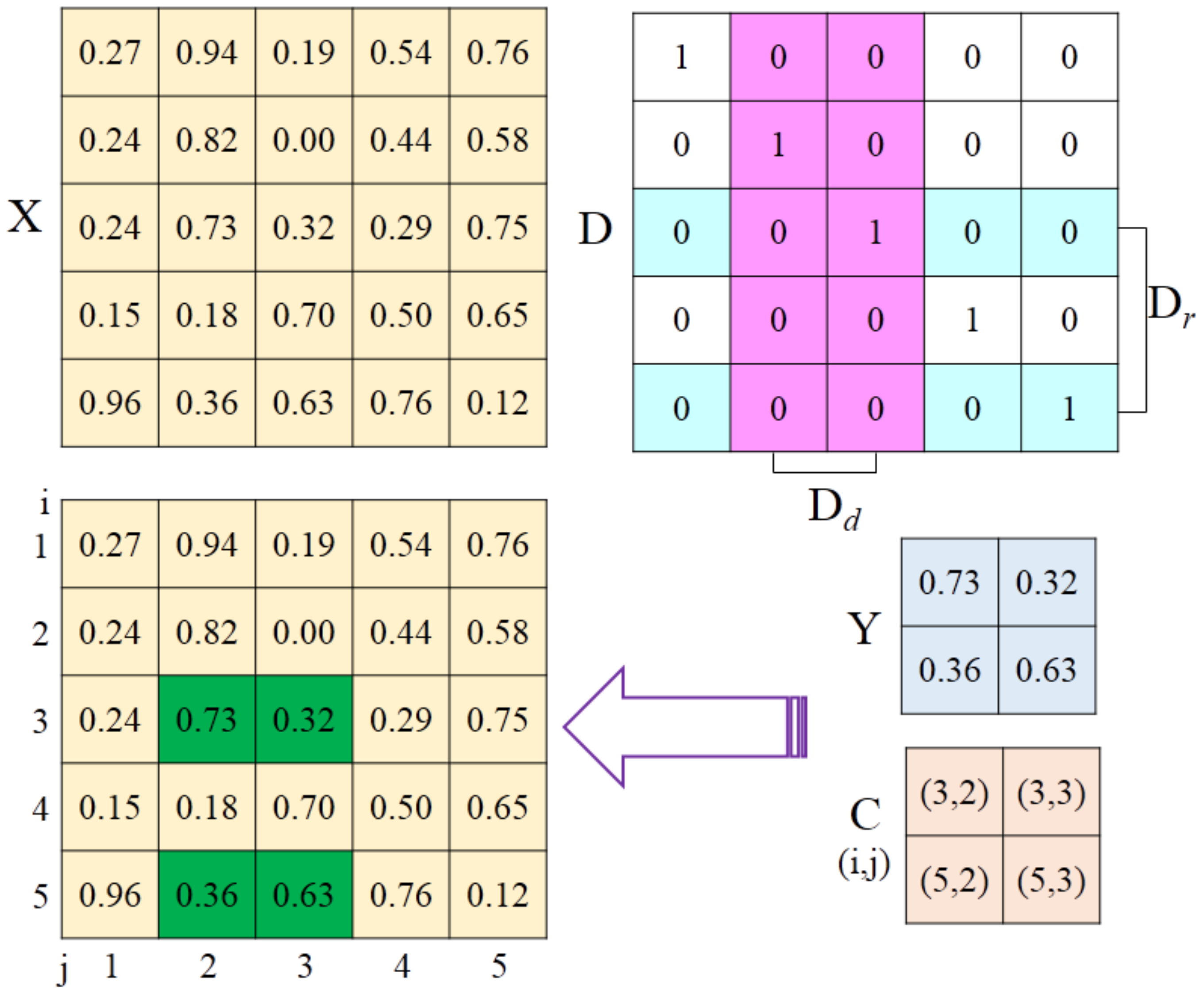
Figure 2.
The results of recovering a synthetic 2D sparse signal using the 2D normalized iterative hard thresholding (2D-NIHT) algorithm. (a) The original signal; (b) The recovered signal; (c) The curve of error versus iterations.
Figure 2.
The results of recovering a synthetic 2D sparse signal using the 2D normalized iterative hard thresholding (2D-NIHT) algorithm. (a) The original signal; (b) The recovered signal; (c) The curve of error versus iterations.
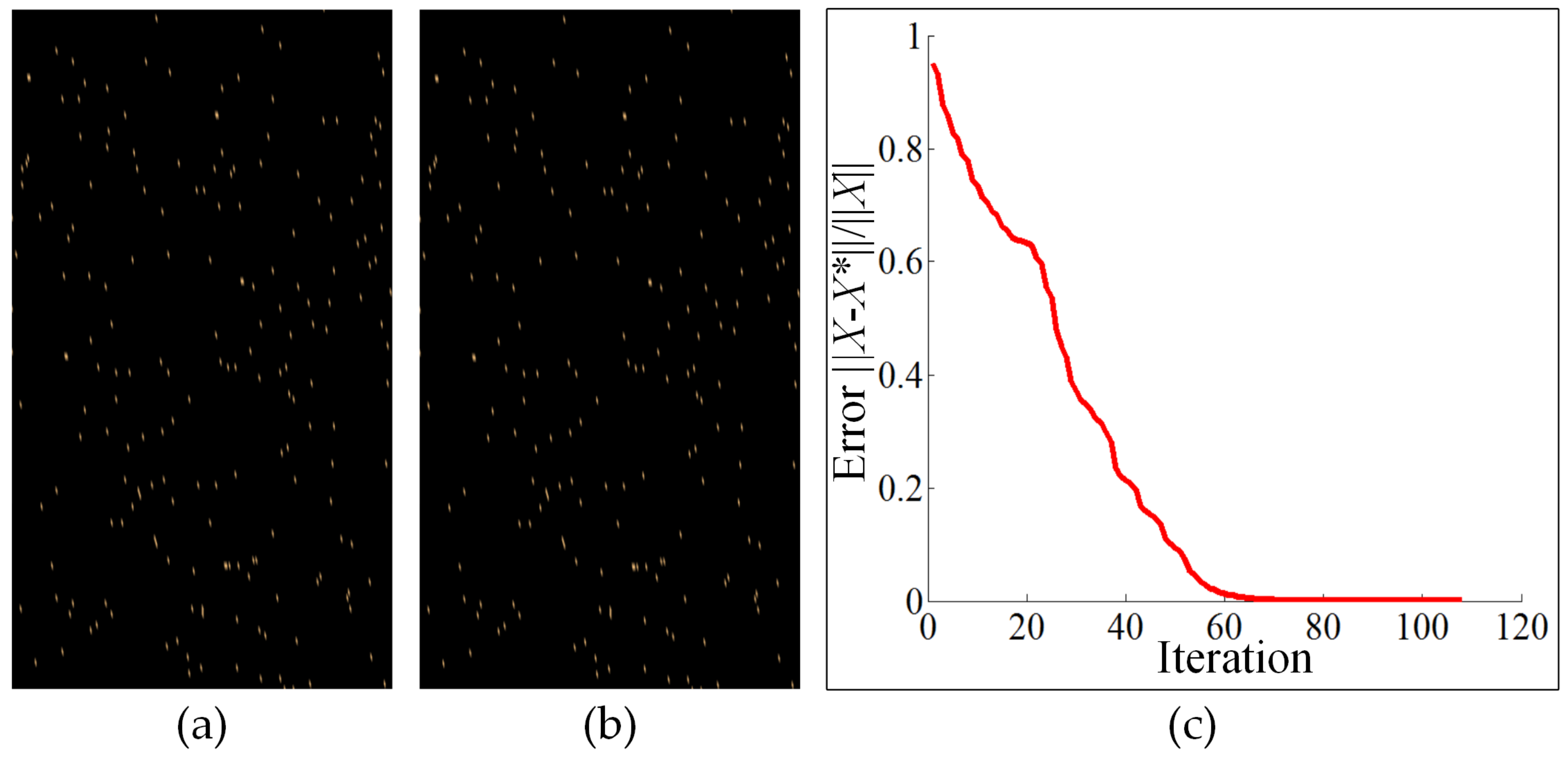
Figure 3.
Comprehensive comparison of reconstruction performance between the 2D-NIHT algorithm and the NIHT algorithm. (a) The comparison of the probability of exact recovery and the computational complexity of the 2D-NIHT and NIHT algorithms under different sparsities; (b) The comparison of the probability of exact recovery and the computational complexity of the 2D-NIHT and NIHT algorithms under different lengths of measurement. Note: “Pro_2D” and “Pro_1D” denote the probability of exact recovery for the 2D-NIHT algorithm and the NIHT algorithm, respectively; “Time_2D” and “Time_1D” denote the reconstruction time of the 2D-NIHT algorithm and the NIHT algorithm, respectively.
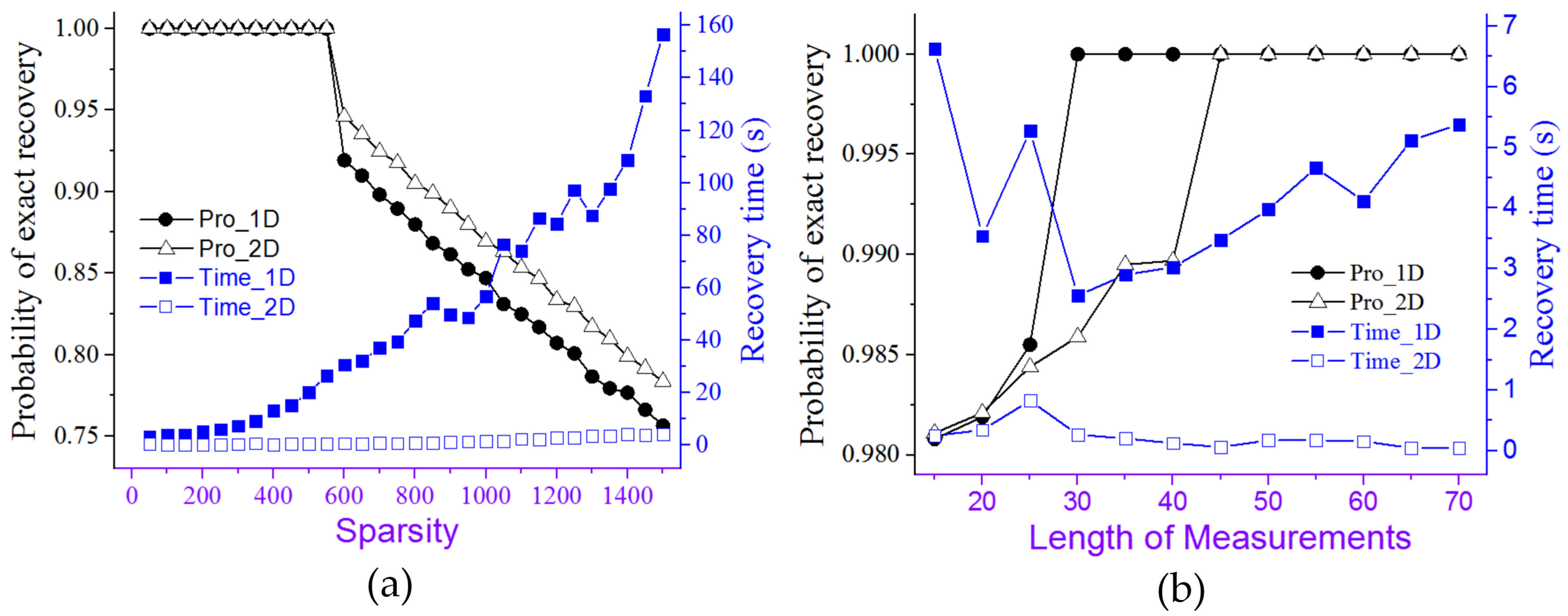
Figure 4.
The original radar scenes. (a) 11 point targets; (b) A helicopter acquired by a SAR system.
Figure 4.
The original radar scenes. (a) 11 point targets; (b) A helicopter acquired by a SAR system.

Figure 5.
The imaging results of two scenes with different SNR levels of noises using a 2D-NIHT algorithm. (a) Imaging results of the 11 point targets at different SNR levels; (b) Imaging results of the helicopter at different SNR levels.
Figure 5.
The imaging results of two scenes with different SNR levels of noises using a 2D-NIHT algorithm. (a) Imaging results of the 11 point targets at different SNR levels; (b) Imaging results of the helicopter at different SNR levels.


Table 1.
Comparison of the five algorithms, including CoSaMP, SL0, BCS, NIHT and 2D-NIHT algorithms, in terms of reconstruction time and probability of exact recovery.
Table 1.
Comparison of the five algorithms, including CoSaMP, SL0, BCS, NIHT and 2D-NIHT algorithms, in terms of reconstruction time and probability of exact recovery.
| CoSaMP | SL0 | BCS | NIHT | 2D-NIHT | ||
|---|---|---|---|---|---|---|
| 11 point targets | Recovery time (s) | 0.069 ± 0.134 | 30.80 ± 1.64 | 0.049 ± 0.024 | 0.629 ± 0.115 | 0.055 ± 0.037 |
| Probability of exact recovery | 1 | 1 | 0.652 ± 0.038 | 1 | 1 | |
| helicopter | Recovery time (s) | 128.79 ± 3.495 | 34.679 ± 0.902 | 0.172 ± 0.044 | 5.176 ± 0.13 | 0.237 ± 0.139 |
| Probability of exact recovery | 0.976 | 1 | 0.476 ± 0.020 | 0.976 | 1 | |
© 2017 by the authors. Licensee MDPI, Basel, Switzerland. This article is an open access article distributed under the terms and conditions of the Creative Commons Attribution (CC BY) license (http://creativecommons.org/licenses/by/4.0/).
Share and Cite
MDPI and ACS Style
Li, G.; Yang, J.; Yang, W.; Wang, Y.; Wang, W.; Liu, L. 2D Normalized Iterative Hard Thresholding Algorithm for Fast Compressive Radar Imaging. Remote Sens. 2017, 9, 619. https://doi.org/10.3390/rs9060619
AMA Style
Li G, Yang J, Yang W, Wang Y, Wang W, Liu L. 2D Normalized Iterative Hard Thresholding Algorithm for Fast Compressive Radar Imaging. Remote Sensing. 2017; 9(6):619. https://doi.org/10.3390/rs9060619
Chicago/Turabian StyleLi, Gongxin, Jia Yang, Wenguang Yang, Yuechao Wang, Wenxue Wang, and Lianqing Liu. 2017. "2D Normalized Iterative Hard Thresholding Algorithm for Fast Compressive Radar Imaging" Remote Sensing 9, no. 6: 619. https://doi.org/10.3390/rs9060619
Note that from the first issue of 2016, this journal uses article numbers instead of page numbers. See further details here.