Satellite Observations of El Niño Impacts on Eurasian Spring Vegetation Greenness during the Period 1982–2015


1
Nansen-Zhu International Research Centre, Institute of Atmospheric Physics, Chinese Academy of Sciences, Beijing 100029, China
2
Department of Atmospheric and Environmental Sciences, University at Albany, State University of New York (SUNY), Albany, NY 12222, USA
3
University of Chinese Academy of Sciences, Beijing 100049, China
4
Collaborative Innovation Center on Forecast and Evaluation of Meteorological Disasters, Nanjing University of Information Science & Technology, Nanjing 210044, China
*
Author to whom correspondence should be addressed.
Remote Sens. 2017, 9(7), 628; https://doi.org/10.3390/rs9070628
Submission received: 25 April 2017
/
Revised: 8 June 2017
/
Accepted: 14 June 2017
/
Published: 22 June 2017
(This article belongs to the Special Issue Remote Sensing of Land-Atmosphere Interactions)
Abstract
:As Earth’s most influential naturally-recurring sea and atmospheric oscillation, ENSO results in widespread changes in the climate system not only over much of the tropics and subtropics, but also in high latitudes via atmospheric teleconnections. In the present study, the linkages between springtime vegetation greenness over Eurasia and El Niño are investigated based on two long-term normalized difference vegetation index (NDVI) datasets from 1982 to 2015, and possible physical mechanisms for the teleconnections are explored. Results from the Empirical Orthogonal Function (EOF) and Singular Value Decomposition (SVD) analyses consistently suggest that the spatial patterns of NDVI, with “negative-positive-negative” values, have closer connections to El Niño. In particular, East Russia is identified as the key region with the strongest negative influences from Eastern Pacific (EP) El Niño on spring vegetation growth. During EP El Niño years, suppressed convection over the Bay of Bengal (BoB) may excite a Rossby wave from the BoB to the Far East. East Russia is located in the west of a large cyclone anomaly accompanied by the strong North and Northwesterly wind anomalies and the transport of cold air from Siberia. As a result, surface air temperature decreases significantly over East Russia and thus inhibits the vegetation growth during spring in the EP El Niño years.
1. Introduction
Eurasia covers more than 1/3 of the Earth’s total land area and is recognized as the largest continent. Eurasian ecosystems over mid- to high-latitudes play a key role in the regional and global climate system through various biophysical and biogeochemical processes and feedback [1,2,3,4,5,6,7,8,9]. For example, the thick taiga vegetation over the extensive area should have a great potential to provide water vapor to the atmosphere through its transpiration activity [10]. Pronounced warming across most of the Northern high latitudes has attracted wide attention to understanding these processes and feedback in recent years [11,12,13,14,15]. To quantify the spatial and temporal variations in vegetation activity, the Normalized Difference Vegetation Index (NDVI) [16] calculated from the near-infrared and red visible reflectance in satellite images has been widely used as an indicator of vegetation greenness to quantify vegetation dynamics [17,18,19].
The impact of atmospheric circulation variability on surface climate and vegetation activity over Eurasia has been investigated on regional and global scales in previous studies [20,21,22,23,24]. In particular, special attention has been devoted to investigating relationships between vegetation dynamics and the North Atlantic Oscillation (NAO) and Arctic Oscillation (AO) [25,26,27], which are the two major patterns of atmospheric variability in the Northern Hemisphere. For example, Li et al. [27] found that a positive winter NAO tends to increase spring vegetation growth over Eurasia. However, little is known about the potential effects of tropical climate anomalies on Eurasian vegetation growth.
El Niño/Southern Oscillation (ENSO) events originate in the low latitudes over the Pacific Ocean but have extensive impacts on large-scale weather and climate systems [28,29,30]. There is increasing evidence that ENSO has strong effects on the vegetation growth and animal populations in a wide range of ecosystems [31,32,33]. However, most research is focused on the core regions that are influenced by ENSO directly such as Africa and the Amazon [34,35,36,37,38]. For example, Ropelewski and Halpert [39] examined the global and regional patterns of precipitation anomalies associated with ENSO and found that, during an El Niño episode, rainfall dramatically increased in certain areas, whereas severe droughts occurred in other regions induced by circulation anomalies in low latitudes. Dillon and Rundel [40] investigated the botanical response of the African desert to the 1982−1983 El Niño event, and examined the interannual variability of vegetation activity over Africa and its relation to ENSO from 1986 through 1990. Holmgren and Scheffer [41] put forward a theoretical framework showing that ENSO could be used in combination with grazer control to restore degraded arid ecosystems as the rainy conditions during ENSO events can trigger the regeneration of woody vegetation in many arid ecosystems.
As Earth’s most influential naturally-recurring sea and atmospheric oscillation, ENSO results in widespread changes in the climate system not only over much of the tropics and subtropics, but also in high latitudes via atmospheric teleconnections [42,43,44,45,46]. Li [47] indicated that anomalistic circulation in the Northern Hemisphere caused by El Niño events can lead to enhancing Westerlies and thus result in warmer weather and weaker winter monsoon in East Asia. Fu et al. [48] found, based on the historical record analysis, that surface air temperature (SAT) in the Northeastern China is strongly influenced by ENSO events, and the occurrence of extremely cold summers is linked to El Niño events. Wang [49] revealed the instability in the relationship between the East Asian summer monsoon and the ENSO cycle in terms of long-term variations.
This study aims to use long-term remote sensing data to detect and attribute the impacts of El Niño forces on the characteristics of Eurasian vegetation dynamics. We explore the linkage between spring (April–May, AM) vegetation in boreal Eurasia (40°–70°N, 0°–150°E) and mature El Niño events during December–January–February (DJF) and uncover relevant physical mechanisms. To achieve this goal and ensure reliability of results, we utilized two of the longest records of satellite measured vegetation greenness products for the period 1982–2015 to quantify vegetation activities. The remainder of the paper is divided into five sections. The materials and methods employed are described in Section 2. The spatiotemporal variability of the Eurasian vegetation and its relationship with El Niño are analyzed in Section 3. Possible physical mechanisms responsible for the El Niño–NDVI relationships are discussed in Section 4, and the discussion and conclusions are provided in Section 5 and Section 6, respectively.
2. Materials and Methods
2.1. NDVI and Climate Data
Satellite-based NDVI datasets have been produced to provide large-scale monitoring of vegetation dynamics for over three decades from the Advanced Very High Resolution Radiometer (AVHRR) sensors [50]. AVHRR’s two channels, near-infrared (NIR) and red (RED), have been combined into spectral indices that directly relate to vegetation characteristics including chlorophyll contents and plant photosynthesis [3,5,11,19,51,52,53]. NDVI is a normalized vegetation index, NDVI = (ρNIR − ρRED)/(ρNIR + ρRED), where ρNIR and ρRED are the surface reflectance in NIR and RED, respectively. It ranges from −1.0 to 1.0 and increases with the amount and cover of green vegetation [54,55]. Here we use two of the long-term NDVI datasets, the 3rd Generation GIMMS NDVI (referred to as NDVI3g) and the NOAA STAR-NESDIS smoothed NDVI (referred to as NDVIsn), based on the AVHRR sensors to detect vegetation activities from 1982 to 2015. NDVI3g is an improved version of 1st Generation NDVI [55] at 1/12° resolution and NDVIsn is originally processed as weekly composites at a spatial resolution of 16 km [56]. Main characteristics of these two datasets are listed in Table 1. The maximum-value composite (MVC) method [57,58] was adopted to generate both NDVI datasets. This method minimizes the non-vegetation influences on NDVI from clouds, aerosols, and other residual atmospheric effects that contaminate the NDVI values [3,5]. Although the same input of satellite measured radiances is used, different data processing methods are applied to each NDVI dataset to remove long-term artifacts associated with satellite drift/changeover, sensor degradation and residual atmospheric effects. Scheftic et al. [50] intercompared seven NDVI products (including NDVI3g and NDVIsn) over the U.S. and Mexico based on linear regression and trend analysis. They found that the spatial patterns in temporal correlations are very consistent across the study region except some arid and mountainous regions, and the temporal variations in spatial correlation of NDVI show high correlation for the entire time period. Despite the overall consistency among all the seven NDVI products, NDVIsn differed from the others because it is the only AVHRR-based dataset that has not been adjusted to match the range of MODIS as has been done with NDVI3g. Here, we analyze these two different NDVI datasets, NDVI3g and NDVIsn, to demonstrate that our results are independent on the NDVI data set used and our detected ENSO impact signals on vegetation activity are robust.
Climate variables that influence vegetation activities are taken from the European Centre for Medium Range Weather Forecasts (ECMWF) Interim reanalysis [59] for the period 1982–2015 (in the same time span of the NDVI data sets). The variable utilized included monthly mean geopotential height, sea surface temperature (SST), u and v wind vectors, 2 m height surface air temperature (SAT) at the spatial resolution of 1° × 1°. The Global Precipitation Climatology Project (GPCP) monthly precipitation dataset from the Climate Prediction Center (CPC) at a 2.5° × 2.5° resolution is also used.
Every El Niño event has somewhat different and distinct characters. Simply characterizing different El Niño types, as seen in the different structure of individual events and their evolution, has been measured through SST anomaly (SSTA) indices in different parts of the tropical Pacific [60]: the Niño3 index (5°N–5°S, 150°–90°W), the Niño3.4 index (5°N–5°S, 170°–120°W), the Niño4 index (5°N–5°S, 160°E–150°W), and the Niño1+2 index (0°–10°S, 90°–80°W). The Bivariate ENSO Timeseries (BEST) index is designed to be simple to calculate and to provide a long-term period ENSO index for research purposes [61]. The Niño3.4 SST and Southern Oscillation Index (SOI) are normalized and combined in the BEST index. These Niño indices are classical and common to define diverse types of El Niño events (e.g., Eastern Pacific El Niño, Central Pacific El Niño and so on) as done in previous studies [62,63,64,65]. All the monthly datasets of various ENSO and oscillation indices, including Niño1+2, Niño3, Niño3.4, Niño4, BEST, AO and NAO, are obtained from the NOAA-CPC as well. All of the indices used in this study are calculated from the seasonal running mean of the wintertime.
2.2. Data Processing
As this study aims to investigate the large-scale features in spring NDVI variations and their associations with El Niño over Eurasia, we first reproject the two NDVI datasets into the monthly coarse resolution 1° × 1° datasets to suppress local scale NDVI variability and data noise/uncertainty. Our study region is limited to the mid-high latitudes over Eurasia (40°–70°N, 0°–150°E). The original NDVI3g is upscaled from 1/12° grid cells to 1° through an averaging of all polygons that intersect each 1° grid cell weighted by the area of polygons within each cell. The original NDVIsn is downscaled from 0.144° grid cells to 1° using bilinear interpolation [50]. Considering that springtime is the most sensitive season for vegetation growth to climate change [66,67,68] and March is still too cold to enable vegetation growth over Eurasia [56], the NDVI seasonal mean in this study is averaged for the two months of April and May to represent boreal spring Eurasian vegetation activities, which is consistent with previous studies [69,70]. In total, each 1° × 1° cell has 34 years of spring mean NDVI (n = 34, which represents the sample size) for the period 1982−2015.
2.3. Methods of Spatiotemporal Pattern Analysis
To investigate the spatially coherent patterns of temporal variations of vegetation, the Empirical Orthogonal Function (EOF) analysis is first conducted for the NDVI. The EOF analysis is considered to be an effective way of analyzing temporally varying spatial patterns of any fields of interest over a specified area [71]. Then, the Singular Value Decomposition (SVD) analysis is also conducted to NDVI, SAT, and precipitation with the SST over tropical Pacific to explore their relationships. SVD is a fundamental matrix operation, a generalization of the diagonalization procedure, and is available in almost every linear algebra or statistics software package. It is first used in a meteorological context by Prohaska [72] to document the simultaneous relationships between monthly mean surface air temperature over the United States and hemispheric sea level pressure patterns. After that, this technique has been widespread used for resolving such problems as the association between two different geophysical variables for decades [73,74,75,76]. In the SVD analysis, each pair of spatial patterns describe a fraction of the squared covariance (i.e., the ratio of each squared singular value to the to the total squared covariance) between two variables (i.e., spring NDVI or climate variables with winter SST in the present study), while the temporal correlation between the corresponding pairs of PC (expansion coefficients) time-series indicates the degree of coupling between two variables [77]. Therefore, the SVD technique can provide means of separating coupled modes of variability between NDVI and SST and identifying their relationships. In order to attribute the effects of El Niño on spring vegetation activity, atmospheric circulation and related climate variables such as temperature and precipitation, are investigated using correlation and composite anomaly analysis methods as well. The statistical significance is determined by the Student’s t-test.
3. Linkage between El Niño and Spring NDVI over Eurasia
3.1. Spatiotemporal Patterns of Spring NDVI
We first examine the 34-year spring NDVI climatology of over Eurasia. The spatial distributions of spring NDVIsn (Figure 1) indicate a variety of biomes over this region. The zones of 35°–50°N and 70°–75°N have low NDVI values (<0.10) corresponding to land covers of deserts or tundra and alpine tundra. Meanwhile, high NDVI values (>0.45) concentrate in Europe (0°–50°E, 40°–60°N) and East Asia (120°–140°E, 40°–50°N) where coniferous forests and mid-latitude deciduous forests dominate. NDVI ranges between 0.10 and 0.45 over most high-latitudes of Eurasia (0°–150°E, 50°–70°N). Here we mainly focus on the areas with the mean NDVI values during April and May (AM) larger than 0.1 to exclude snow-covered and barren land from our analysis [3,5,78].
We then examine spatiotemporal patterns of spring NDVI over Eurasia via EOF analysis and relate different NDVI_EOF modes to El Niño or other climate indices such as AO and NAO. The first EOF pattern obtained for the period 1982−2015 in NDVIsn (Figure 2a) and NDVI3g (Figure 2e) accounts for about 15.5% and 17.2% of the total spring NDVI variance, respectively. It is noted that positive values are present over most Eurasia except for some areas located in Europe (with negative values in brown) and most of the large positive values (in green) are found in Siberia (80°–120°E, 50°–70°N), indicating relatively stronger variability in Siberia. The time-series of the first EOF (Figure 2b,f) exhibits the characteristic of interannual variability. The second EOF mode (Figure 2c,g) explains about 12.1% (NDVIsn) and 9.9% (NDVI3g) of the total NDVI variance, indicating regional-scale hotspots of relatively stronger variability in vegetation greenness in Eurasia. For this EOF mode, Europe, the Lake Baikal region and East Asia are dominated by large negative values (in brown) while positive values (in green) cover other parts of Eurasia especially in West Siberia, implying that the changes in NDVI over the brown colored regions are opposite to the other areas. The corresponding time-series of EOF2 (Figure 2d,h) displays a period of 2–5 years oscillation in spring NDVI, suggesting a possible connection with ENSO. It also shows that more dramatic changes happened around the mid-1990s, indicating a noticeable climate change related to this EOF mode over Eurasia around this period.
3.2. Correlations between Spring NDVI and El Niño
The above EOF analysis reveals the spatiotemporal patterns of spring NDVI variations over Eurasia, and the first two EOF modes can be considered to represent the primary patterns of vegetation changes during spring. In this section, we further examine the correlation between Eurasian spring NDVI and various El Niño and oscillation indices based on the first two time-series of the EOF modes (Table 2). The first EOF (EOF1) mode of spring NDVI has a statistically significant correlation (p < 0.05) with AO and NAO but not with El Niño indices. However, the second EOF (EOF2) mode is significantly correlated with El Niño indices (especially for Niño3, Niño3.4 and Niño4), and with AO (p < 0.20 for NDVIsn, p < 0.05 for NDVI3g) as well. For example, the correlation coefficients between the EOF2 time-series of NDVIsn and NDVI3g and El Niño indices (after detrending both time-series) are −0.22 and −0.24 (p < 0.20) for Niño3, −0.29 and −0.30 (p < 0.10) for Niño3.4, −0.30 and −0.31 (p < 0.10) for Niño4, respectively.
We further calculate the correlation coefficient to validate the above relationship between NDVI and Niño indices (Niño3, Niño3.4 and Niño4 indices) at the grid level (Figure 3). Evidently different Niño indices are significantly correlated to spring NDVI over different areas in Eurasia. Niño4 (Figure 3a,b), which can be used to represent the Central Pacific (CP) Niño events, shows the strongest correlation in Europe (west to 70°E), while Niño3 (Figure 3e,f), which can capture most of the Eastern Pacific (EP) Niño events, has the strongest influence in East Russia (90°–130°E, 50°–65°N). The correlation patterns between NDVI and Niño3.4 (Figure 3c,d) seem to combine the correlative results from Niño3 and Niño4 indices. Nevertheless, all three Niño indices generally exhibit similar correlation patterns with spring NDVI over Eurasia, which are quite similar to the second EOF mode (Figure 2c,g).
The above results suggest that El Niño may be responsible for the negative NDVI anomalies over West Europe (20°–40°E, 40°–60°N) and East Russia (90°–130°E, 50°–65°N), and for the positive NDVI anomalies over East Europe (50°–80°E, 40°–70°N) as well. However, we cannot ignore the impacts of NAO and AO on spring NDVI over Eurasia considering their strong correlation coefficients shown in Table 2. Therefore, we identify next the regions where El Niño exerts the considerable influence on spring NDVI variations.
3.3. Relationship between Spring NDVI Changes and Winter SSTA over Equatorial Pacific
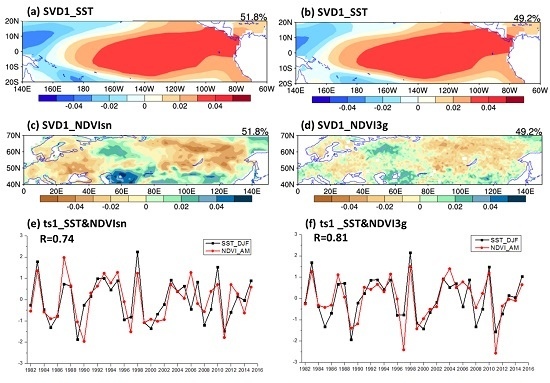
In this section, we further examine the relationship between interannual variations of spring NDVI over Eurasia and winter SSTA over equatorial Pacific from the first two covariance matrix fields using the SVD analysis for the period from 1982 to 2015. Figure 4 shows the spatial patterns and time-series of the first leading paired modes of SST-NDVI based on the NDVIsn and NDVI3g datasets, respectively. The first modes both explain about 50% of the total squared covariance between the two fields and their first time-series has a significant correlation of 0.74 (p < 0.001) for NDVIsn and 0.81 (p < 0.001) for NDVI3g. The first mode of winter SST (Figure 4a,b) shows a broad band of warm SST phase developing in the central to eastern equatorial Pacific, displaying the typical feature of an El Niño event. The corresponding NDVI patterns (Figure 4c,d) are characterized by positive values over East Europe (50°–80°E, 40°–70°N) and the semi-arid regions south to Russia (50°–130°E, 40°–50°N), and by negative values over West Europe (20°–40°E, 40°–70°N) and most East Russia (80°–130°E, 50°–70°N), which are quite similar to the spatial patterns of EOF2 obtained from spring NDVI (Figure 2c,g). The time-series of SVD1 show significant interannual fluctuations with a period of 3–5 years both in SST and NDVI (Figure 4e,f). In particular, we can also detect some peaks coupled with the well-known El Niño events in years of 1983, 1998 and 2010, respectively, from the time-series of SST and NDVI. The similarities between the first paired SVD-NDVI spatial mode and the second EOF spatial mode of NDVI and the strong correlation coefficients between SVD1 time-series of SST and NDVI suggest that the spatial patterns of “negative-positive-negative” NDVI changes from west to east over Eurasia are positively and remotely linked with the winter SSTA over equatorial Pacific.
However, the second EOF mode of NDVI explains only about 10% of the total variance in spring NDVI over Eurasia. It is important to notice that Eurasia is a huge continent and different climate processes affect vegetation activities over different regions. Therefore, it is necessary to identify the primary regions that have the strongest influences from El Niño on the spring NDVI in Eurasia. It is well known that there are close connections between Eurasian climate and large-scale circulation systems in mid-high latitudes such as AO and NAO [79,80,81,82,83,84]. For example, Hurrell [85] revealed that the NAO modulates wintertime SAT over much of Eurasia, with positive polarity of the NAO being associated with positive SAT anomalies extending from Great Britain and Scandinavia far into Siberia. Rigor et al. [86] also suggested that the AO accounted for more than half of the SAT trends over Alaska, Eurasia and the Eastern Arctic Ocean during the past two decades. These changes in SAT due to NAO and AO are expected to influence the Eurasian spring NDVI over some particular regions. Here we calculate the correlations between spring NDVI and winter AO (Figure 3g,h) and NAO (Figure 3i,j) to identify these particular regions. Both winter NAO and AO exert similar impacts on spring NDVI with the dramatic positive anomalies spreading over central Eurasia from Europe to Lake Baikal (0°–100°E, 45°–60°N) and negative anomalies on East European Plain (40°–60°E, 55°–65°N) and North Siberia (85°–130°E, 65°–70°N). Comparing to the correlations between spring NDVI and winter Niño indices (Figure 3a–f), East Russia (80°–130°E, 50°–70°N) can be identified as the regions with the strongest influences from El Niño and the least impacts from NAO and AO. Therefore, we focus our remaining analysis on the spring NDVI variations in East Russia.
Figure 5 displays co-variability patterns and time-series of the first leading paired modes between winter SST over equatorial Pacific and spring NDVI over East Russia. The first leading paired modes explain about 74.3% (NDVIsn) and 77.2% (NDVI3g), respectively, of the total squared covariance in the SST-NDVI SVD fields, and the corresponding two time-series have a statistically significant correlation of 0.50 and 0.51 (p < 0.01). Dominant positive SST values are found over Eastern equatorial Pacific (80°–160°W, 20°S–10°N) both in Figure 5a,b with the most significant centers located around 140°–155°W. The corresponding NDVI anomalies are both negative over the identified key regions, which is consistent with Figure 3 and Figure 4. The most notable negative anomalies occur in north and east to the Lake Baikal in the NDVIsn dataset. Such NDVI spatial patterns can explain about 31.1% (NDVIsn) and 35.2% (NDVI3g) of the total variance in the spring NDVI, representing the major pattern of NDVI variability over East Russia. By comparing the difference of first spatial pattern of SVD-SST from Figure 4 and Figure 5, we notice that the SST pattern in Figure 5 is more focused on the East Pacific (east to 160°W) than in Figure 4 (east to 180°). This difference indicates that the NDVI anomalies of East Russia (referred to as ERNDVI hereafter) are more relevant to the SSTA over East Pacific (EP El Niño), which is consistent with the conclusion in Section 3.2. We also calculate the correlation coefficients between the time-series of SVD_ERNDVI-SST and various Niño, and AO, NAO indices (Table 3). Again, the time-series of SST is mostly correlated to Niño3 and Niño3.4, while the time-series of ERNDVI has a stronger connection with Niño3 than other indices in both NDVI datasets. As expected, NAO and AO have little influences on spring ERNDVI comparing with the Niño indices. Therefore, these results support that ERNDVI has close teleconnections with EP El Niño events.
4. Possible Physical Mechanisms for the Teleconnection between ERNDVI and El Niño
4.1. Climatic Impacts on ERNDVI
As temperature and precipitation are the most important climate controls on vegetation growth in Northern high latitudes [3,5,87], we first explore the responses of temperature and precipitation to El Niño over East Russia and their impacts on NDVI. Figure 6 displays the co-variability patterns and time-series of the first leading paired modes between winter SST over equatorial Pacific and spring SAT and precipitation over East Russia via the SVD analysis, which explain about 80.5% (SAT) and 48.3% (precipitation), respectively, of the total squared covariance, with the correlations of 0.47 (p < 0.005) and 0.58 (p < 0.001) between the PC time-series, respectively. Both SST patterns (Figure 6a,b) demonstrate the characteristics of El Niño with positive anomalies emerging over the tropical central to Eastern Pacific. The corresponding SAT patterns (Figure 6c), which explain 48.9% of the total variance, are dominated by negative values across East Russia. However, the SVD1 pattern of precipitation (Figure 6d) only accounts for 11.4% of the total variance with positive values in the regions south to 65°N over most of East Russia and the negative values covering regions in the north. In addition, we calculate the correlation coefficients between the spring ERNDVI and the time-series of first leading SVD mode in SAT and precipitation fields at each grid cell (figures not shown). Results also prove that ERNDVI depends more on SAT than precipitation, which is in agreement with previous studies [3,5,13,88]. Ebata and Tateishi [89] indicated that vegetation in the 110°E transect over Siberia has a high positive (0.92) correlation between SAT and vegetation meridional profile, suggesting that the dominant factor for the NDVI profile is temperature in the forest-tundra transect. Los et al. [90] also observed a very strong connection between the anomalies in NDVI and SAT, but weaker associations with precipitation in some regions. It is expected that sufficient soil water is available for plant growth contributed by snow and ice melting during spring. Therefore, temperature is primarily the controlling climate factor throughout the spring vegetation growth over East Russia.
4.2. Impacts of Atmospheric Teleconnections of El Niño on Spring ERNDVI
In this section, we explore how El Niño affects vegetation growth over East Russia by controlling climate variations during springtime via atmospheric teleconnections. As the analysis in Section 3.3 indicates that ERNDVI has close connections to the EP El Niño events, we perform composite analysis by choosing several EP El Niño years according to Niño3 index as done previously [91]. We define the mature EP El Niño events as the years when the normalized winter Niño3 index has a standard deviation greater than 1.0, including 1982–1983, 1986–1987, 1992–1993, 1997–1998, 2002–2003, 2006–2007 and 2014–2015, and composite the anomalies of NDVI, temperature and precipitation during springtime after the mature EP El Niño events (i.e., 1983, 1987, 1993, 1998, 2003, 2007, 2015). Figure 7a composites the spring ERNDVIsn anomalies in the EP El Niño years with significant negative anomalies spreading north and east to Lake Baikal (100°–135°E, 50°–65°N), southeast of Russia. Similar anomalous patterns can also be found in the composite anomalies of spring SAT in the EP El Niño years (Figure 7b). As for precipitation (Figure 7c), positive anomalies cover most south to 65°N in East Russia while negative anomalies dominate the north. It is clear that the ERNDVI anomalies depend more on temperature than on precipitation, which is consistent with the aforementioned results.
Next, we focus on how the EP El Niño events influence the spring temperature over East Russia. As atmospheric circulation controls regional SAT patterns, we analyze the variations in spring atmospheric wind fields. The composite anomalies of 200, 500 and 850 hPa spring winds in the EP El Niño years are shown in Figure 8a–c. The southeast of Russia (the regions in the red frame), which exhibits the most significant NDVI anomalies, is located west of a large cyclone anomaly spreading from Lake Baikal to North Pacific with the core in the Kamchatka peninsula, accompanied by the strong North and Northwesterly wind anomalies and the transport of cold air from Siberia at the same time. In addition, during the EP El Niño years, the barotropic circulation anomalies over East Eurasia and West Pacific are also seen in Figure 8, with an “anticyclone–cyclone–anticyclone–cyclone” meridional structure over “the Bay of Bengal–Southwest China–South Japan–Kamchatka peninsula”, especially in the upper troposphere (Figure 8a,b). The cyclone anomaly over the Kamchatka peninsula is the largest and northernmost part of the meridional atmospheric circulation anomalous structure. According to the previous studies, the development and persistence of the circulation anomalies over Northwest Pacific have a close relationship with El Niño [92,93]. For example, Zhang et al. [94] attributed the anticyclonic anomaly over Northwest Pacific to a Rossby wave response to the anomalous cooling over the Maritime Continent during the mature El Niño phase. Xie et al. [95] also revealed that the suppressed convection in the subtropical Northwest Pacific, which results from El Niño, can excite a meridional teleconnection and further affect the summer climate over East Asia. Because the atmospheric circulation anomalies display a Rossby-wave-like meridional structure (Figure 8), we analyze the wave activity flux at 200 hPa (Figure 9a) to identify the wave source and its propagation path following the approaches of Takaya and Nakamura [96,97]. Takaya and Nakamura [97] introduced a new formulation of an approximate conservation relation for stationary Rossby waves on a zonally varying basic flow, utilizing that A (proportional to wave enstrophy) and ε (proportional to wave energy) are both related to the wave activity pseudomomentum. The arrows in Figure 9a clearly show that the Rossby wave propagates northeastward from the Bay of Bengal, through Southwest China and South Japan, to the large regions around the Kamchatka peninsula (110°E–170°W, 50°–65°N), which leads to the significant anomalous low pressure (gray shadow) from Lake Baikal to the Far East. These patterns are consistent with the atmospheric circulation anomalies shown in Figure 8. The Rossby wave can also be found from the composite anomalies of 200 hPa geopotential height as well (Figure 9c), which show the “positive–negative–positive–negative” anomalies located in the propagation path along with the “Bay of Bengal–Southwest China–South Japan–Kamchatka peninsula”.
According to the wave activity flux at 200 hPa, we deduce that the wave source is located in the Bay of Bengal (BoB) where convection is suppressed (Figure 10a) during springtime. Wu et al. [98] discovered the largest rainfall anomalies in the BoB during boreal spring. Typically, El Niño develops during boreal summer, peaks during early winter, and decays the following spring. As for the “delayed” influence of El Niño, Xie et al. [95] proposed one of the most important possible mechanisms named the “Indian Ocean capacitor effect”: much of the tropical Indian Ocean (TIO) warms up following the El Niño peak because of the downwelling ocean Rossby waves in the southwestern basin [99,100] and heat flux changes elsewhere induced by ENSO [101,102]. El Niño is in a positive phase when the SST is anomalously cool in the west and warm in the east of Pacific after a rapid development during the boreal winter. After a mature El Niño with the Indian Ocean warming, the equatorial wind anomalies are Easterlies from the West Pacific to the North Indian Ocean (NIO), which develops in winter and strengthens in the following spring, with the wind coupled to the SST in the sense that it blows from the cooler waters toward the warmer waters [103]. Then the SST cooling over NIO is also contributed by the increased surface wind speed and enhanced upward latent heat flux associated with the significant anomalous Easterlies (Figure 8c). This latent heat flux anomaly favors further cooling of SST over NIO during boreal spring and provides a positive wind-evaporation-SST (WES) feedback [98,104]. The persistent SST cooling anomalies over NIO and the SST warming over TIO develop the equatorially asymmetric Indian Ocean Mode contributed by the cross-equatorial SST gradient, resulting in the atmosphere and rainfall anomalies as well [98,105]. Precipitation decreases (increases) with Northeasterly (Northwesterly) wind anomalies in north (south) of the equator over TIO [100]. Kawamura et al. [106] further used an ocean general circulation model forced by daily mean wind stresses and heat fluxes to examine possible roles of the TIO in the Asian summer monsoon and ENSO coupling. They found the westward extension of anomalously suppressed convection from the vicinity of the Philippines into the NIO from the preceding winter to spring, which has a signal of ENSO and can be viewed as a developing process of WES feedback. The persistence of WES feedback affects the land surface hydrologic processes in the Asian continent through a Rossby wave response to the anomalous convective heating. Kawamura et al. [106] also drew a conclusion that the WES feedback in the TIO serves as a bridge between the ENSO prevailing in the preceding winter and the anomalous summer monsoon.
In Figure 10a, the composite anomalies of tropical rainfall over the BoB are indeed significantly negative during the EP El Niño years in springtime. We also define a BBR (Bay of Bengal rainfall) index, calculated from the regional mean rainfall over the BoB (85°–95°E, 5°–15°N), which exhibits the strongest correlation with El Niño in Figure 10b, to determine its relationships with El Niño and the Rossby wave. Evidently, the time-series of BBR has a significant negative correlation of −0.45 (p < 0.01) with the El Niño index. We also composite the anomalies of wind and geopotential height at 200 hPa in low-value BBR years (Figure 9b,d), which include 1983, 1987, 1995, 1997, 1998 and 2011 defined as the years with the standard deviation less than −1.0. In the low-value BBR years, suppressed convection over the BoB can excite the Rossby-wave-like structure from the BoB to Kamchatka peninsula both in the wind (Figure 9b) and geopotential height (Figure 9d) anomalies at 200 hPa, which are quite like the meridional structures formed in the EP El Niño years shown in Figure 8a and Figure 9c.
In terms of how BBR excites Rossby waves, many studies have demonstrated the relationships between tropical thermal forcing and extratropical teleconnection patterns [107,108,109]. As discussed by Held et al. [110], in the tropics, the diabatic heating is mainly balanced by the adiabatic cooling, and the divergent flow associated with the vertical motion induced by heating can be considered as Rossby wave sources. The divergence induced by the tropical heating becomes weaker in midlatitudes and so the effect of vorticity generation by the divergence would not be significant there. However, as latitude increases, the planetary vorticity is also increased, and its effects would become more significant on Rossby wave propagation. In addition, the advection of vorticity by the divergent component of the flow can also be considered as the Rossby wave sources [108], which would displace the wave sources further poleward.
In summary, suppressed convection over the BoB induced by the persistent negative SSTA and WES feedback can excite a Rossby wave from the BoB to the Far East. The strong North and Northwesterly wind anomalies associated with the Rossby wave advect the cold air from Siberia to East Russia, which leads to the remarkable negative SAT anomalies over East Russia and inhibits spring vegetation growth in the EP El Niño years. The possible physical mechanisms are summarized in the schematic diagram shown in Figure 11.
5. Discussion
Our analysis and attribution are primarily statistical and empirical and thus have limitations in establishing the cause-and-effect relationships between Eurasian NDVI and ENSO. In addition, Eurasia is a huge content and various climate systems can affect Eurasian vegetation activities differently over different regions. For example, Buermann et al. [111] indicated that the warm event ENSO signal was manifested as warmer and greener conditions in North America, Far East Asia, and to some extent central Europe, while the positive phase AO signal featured enhanced warm and green conditions over large regions in Europe and Asian Russia for the period 1982–1998. Balzter et al. [112] suggested that the AO and El Niño controlled the forest fire regimes in Central and East Siberia: several extreme fire years in Central Siberia were associated with a highly positive AO phase while several years with high fire damage in East Siberia occurred in El Niño years. Gong and Ho [113] implied that the large-scale circulation was essential for understanding the regional response of vegetation to global climate change; taking nine circulation indices and time lags into account, a large portion (71%) of the satellite-sensed variance in NDVI could be explained.
Our results in Figure 3 show that different Niño events are significantly correlated to spring NDVI regionally over different areas in Eurasia while AO/NAO have a much broader impact on Eurasian NDVI over most areas in 45°–60°N, especially in Europe and east of the Baikal Lake region. As the time-series of ERNDVI has a much stronger connection with Niño3 than other ENSO and oscillation indices in both NDVI datasets, the present paper focuses mostly on exploring the ERNDVI–EP El Niño relationship. However, other mechanisms and teleconnections may play a more important role in NDVI elsewhere. For example, we found that spring NDVI over west and central parts of Eurasia has closer linkage to CP El Niño in Section 3. Graf and Zanchettin [114] analyzed the relationship between CP El Niño and European climate and proposed a tropospheric bridge as the mechanism primarily responsible for the establishment of CP El Niño/negative NAO teleconnection and of associated cold European winters. When the anomalous convective heating occurs near the edge of the warm pool, the subtropical jet (STJ) waveguide can be activated only during CP El Niño events and further enhanced by planetary wave flux divergence in the subtropical upper troposphere, favoring the propagation of a wave number 5 disturbance around the subtropical Northern Hemisphere. This wave contributes to the weakening of the Azores High, and the negative NAO phase and cold European after a mature CP El Niño, which is associated with the negative anomaly patterns of spring NDVI over Europe. Moron and Plaut [115] also revealed the impact of El Niño upon several weather regimes over Europe during 119 winters (1882–2000) using a cluster analysis.
Understanding that vegetation-ENSO interactions have great potential to improve the prediction of short-term vegetation dynamics and ecological variability. Previous studies have shown that large-scale climatic indices can predict ecological processes better than local weather and climate [116,117]. For example, Hallett et al. [118] found that climate indices relating to atmospheric circulation patterns (or teleconnections) may be better predictors of ecological variability because they integrate the co-variations between different drivers of ecological activity. Our results in this study highlight the need and importance for the inclusion of large-scale climate indices in predicting ecological processes over Eurasia. Considering the complex relationships among ENSO, other climatic systems such as NAO and AO, and Eurasian NDVI, we will continue to explore these relationships and related physical mechanisms, both in breadth and depth, in the future work.
6. Conclusions
This work examines the relationships between springtime NDVI over Eurasia and El Niño based on two of the longest NDVI datasets, NDVIsn and NDVI3g, from 1982 to 2015, and explores possible physical mechanisms behind the relationships. It first decomposes spring Eurasian NDVI into independent modes via an EOF analysis and then examines the correlations between various Niño indices and spring Eurasian NDVI based on the first two time-series of the EOF modes, which represent the primary vegetation variation pattern during spring. We further investigate how winter tropical Pacific SSTA and spring climate parameters (i.e., temperature and precipitation) are linked to the spring vegetation growth over Eurasia using a SVD analysis. The major conclusions can be summarized as follows:
- The second EOF mode of spring NDVI, with the “negative-positive-negative” values varying from Europe, West Siberia to East Asia, explains about 12.1% (NDVIsn) and 9.9% (NDVI3g) of the total variance and its time-series is more correlated to the El Niño indices, especially Niño3, Niño3.4 and Niño4, than other climate indices.
- The spatial patterns of correlation coefficients between Eurasian NDVI and different Niño indices also show the patterns of the “negative-positive-negative” values varying from Europe, West Siberia to East Asia, which are similar to the spatial patterns of the second EOF modes obtained from spring Eurasian NDVI.
- Various Niño indices affect spring NDVI changes differently over different areas in Eurasia to various degrees. SSTA in the Niño4 region (CP El Niño events) have closer connections to European NDVI variations (west to 70°E), while SSTA in the Niño3 region (EP El Niño events) impacts primarily East Russian NDVI changes (90°–130°E, 50°–65°N) significantly. The influence of SSTA in the Niño3.4 region seems to have the combined effects of Niño3 and Niño4 indices on Eurasian NDVI variations.
- Temperature anomalies play a leading role as the bridge in explaining the relationship between NDVI and El Niño over Eurasia. The spatial patterns of SST and SAT are similar to those of SST and NDVI via the SVD analysis, exhibiting the “negative-positive-negative” values both in the SAT and NDVI fields from west to east over Eurasia along with an El Niño signal in the SST field.
- East Russia (80°–130°E, 50°–70°N) is identified as the key region with the strongest negative influences from El Niño on spring NDVI growth.
The possible physical mechanisms responsible for the ERNDVI–EP El Niño relationships are summarized as follows. During EP El Niño years, suppressed convection over the BoB, which is associated with the local persistent negative SSTA induced by WES feedback, can excite the Rossby wave with the “anticyclone–cyclone–anticyclone–cyclone” meridional structure both in wind and geopotential height anomalies from the BoB to the Far East. East Russia is located in the west of a large cyclone anomaly spreading from Lake Baikal to North Pacific with the core in the Kamchatka peninsula, accompanied by strong North and Northwesterly wind anomalies and the transport of cold air from Siberia at the same time. As a result, SAT decreases significantly over East Russia and thus inhibits the vegetation growth during spring in the EP El Niño years.
Acknowledgments
This research was jointly supported by the National Natural Science Foundation of China (Grant Nos. 41325018, 41421004, 41575079) and the UCAS (UCAS [2015]37) Joint PhD Training Program, the CAS/SAFEEA international partnership program for creative research team “regional environmental high resolution numerical simulation”.
Author Contributions
Ke Fan and Liming Zhou conceived and designed the experiments and the paper; Jing Li performed the experiments; Liming Zhou and Jing Li analyzed the data; Jing Li wrote the paper.
Conflicts of Interest
The authors declare no conflict of interest.
References
- Bounoua, L.; Collatz, G.; Los, S.; Sellers, P.; Dazlich, D.; Tucker, C.; Randall, D. Sensitivity of climate to changes in NDVI. J. Clim. 2000, 13, 2277–2292. [Google Scholar] [CrossRef]
- Myneni, R.; Dong, J.; Tucker, C.; Kaufmann, R.; Kauppi, P.; Liski, J.; Zhou, L.; Alexeyev, V.; Hughes, M. A large carbon sink in the woody biomass of northern forests. Proc. Natl. Acad. Sci. USA 2001, 98, 14784–14789. [Google Scholar] [CrossRef] [PubMed]
- Zhou, L.; Tucker, C.J.; Kaufmann, R.K.; Slayback, D.; Shabanov, N.V.; Myneni, R.B. Variations in northern vegetation activity inferred from satellite data of vegetation index during 1981 to 1999. J. Geophys. Res. Atmos. 2001, 106, 20069–20083. [Google Scholar] [CrossRef]
- Bogaert, J.; Zhou, L.; Tucker, C.; Myneni, R.; Ceulemans, R. Evidence for a persistent and extensive greening trend in Eurasia inferred from satellite vegetation index data. J. Geophys. Res. Atmos. 2002, 107. [Google Scholar] [CrossRef]
- Zhou, L.; Kaufmann, R.; Tian, Y.; Myneni, R.; Tucker, C. Relation between interannual variations in satellite measures of northern forest greenness and climate between 1982 and 1999. J. Geophys. Res. Atmos. 2003, 108. [Google Scholar] [CrossRef]
- Wang, G.; You, L. Delayed impact of the North Atlantic Oscillation on biosphere productivity in Asia. Geophys. Res. Lett. 2004, 31, L12210. [Google Scholar] [CrossRef]
- Grippa, M.; Kergoat, L.; Le Toan, T.; Mognard, N.; Delbart, N.; L’hermitte, J.; Vicente-Serrano, S. The impact of snow depth and snowmelt on the vegetation variability over central Siberia. Geophys. Res. Lett. 2005, 32, L21412. [Google Scholar] [CrossRef]
- Gutman, G.; Reissell, A. (Eds.) Eurasian Arctic Land Cover and Land Use in a Changing Climate; Springer: Berlin, Germany, 2011. [Google Scholar]
- Chen, H.; Zhang, Y.; Yu, M.; Hua, W.; Sun, S.; Li, X.; Gao, C. Large-scale urbanization effects on eastern Asian summer monsoon circulation and climate. Clim. Dyn. 2016, 47, 117–136. [Google Scholar] [CrossRef]
- Suzuki, R.; Yatagai, A.; Yasunari, T. Satellite-derived vegetation index and evapotranspiration estimated by using assimilated atmospheric data over Asia. J. Meteorol. Soc. Jpn. Ser. II 1998, 76, 663–671. [Google Scholar] [CrossRef]
- Myneni, R.B.; Keeling, C.; Tucker, C.J.; Asrar, G.; Nemani, R.R. Increased plant growth in the northern high latitudes from 1981 to 1991. Nature 1997, 386, 698. [Google Scholar] [CrossRef]
- Wohlfahrt, J.; Harrison, S.; Braconnot, P. Synergistic feedbacks between ocean and vegetation on mid-and high-latitude climates during the mid-Holocene. Clim. Dyn. 2004, 22, 223–238. [Google Scholar] [CrossRef]
- Zhang, X.; Friedl, M.A.; Schaaf, C.B.; Strahler, A.H. Climate controls on vegetation phenological patterns in northern mid-and high latitudes inferred from MODIS data. Glob. Chang. Biol. 2004, 10, 1133–1145. [Google Scholar] [CrossRef]
- Jeong, S.J.; Ho, C.H.; Gim, H.J.; Brown, M.E. Phenology shifts at start vs. end of growing season in temperate vegetation over the Northern Hemisphere for the period 1982–2008. Glob. Chang. Biol. 2011, 17, 2385–2399. [Google Scholar] [CrossRef]
- Peng, S.; Piao, S.; Ciais, P.; Friedlingstein, P.; Zhou, L.; Wang, T. Change in snow phenology and its potential feedback to temperature in the Northern Hemisphere over the last three decades. Environ. Res. Lett. 2013, 8, 014008. [Google Scholar] [CrossRef]
- Tucker, C.J. Red and photographic infrared linear combinations for monitoring vegetation. Remote Sens. Environ. 1979, 8, 127–150. [Google Scholar] [CrossRef]
- Justice, C.O.; Townshend, J.; Holben, B.; Tucker, E.C. Analysis of the phenology of global vegetation using meteorological satellite data. Int. J. Remote Sens. 1985, 6, 1271–1318. [Google Scholar] [CrossRef]
- Moulin, S.; Kergoat, L.; Viovy, N.; Dedieu, G. Global-scale assessment of vegetation phenology using NOAA/AVHRR satellite measurements. J. Clim. 1997, 10, 1154–1170. [Google Scholar] [CrossRef]
- Pettorelli, N.; Vik, J.O.; Mysterud, A.; Gaillard, J.-M.; Tucker, C.J.; Stenseth, N.C. Using the satellite-derived NDVI to assess ecological responses to environmental change. Trends Ecol. Evol. 2005, 20, 503–510. [Google Scholar] [CrossRef] [PubMed]
- Overpeck, J.T.; Rind, D.; Goldberg, R. Climate-induced changes in forest disturbance and vegetation. Nature 1990, 343, 51. [Google Scholar] [CrossRef]
- Heaney, L.R. A synopsis of climatic and vegetational change in Southeast Asia. Clim. Chang. 1991, 19, 53–61. [Google Scholar] [CrossRef]
- Poveda, G.; Salazar, L.F. Annual and interannual (ENSO) variability of spatial scaling properties of a vegetation index (NDVI) in Amazonia. Remote Sens. Environ. 2004, 93, 391–401. [Google Scholar] [CrossRef]
- Roucoux, K.; De Abreu, L.; Shackleton, N.; Tzedakis, P. The response of NW Iberian vegetation to North Atlantic climate oscillations during the last 65kyr. Quat. Sci. Rev. 2005, 24, 1637–1653. [Google Scholar] [CrossRef]
- Scheiter, S.; Higgins, S.I. Impacts of climate change on the vegetation of Africa: An adaptive dynamic vegetation modelling approach. Glob. Chang. Biol. 2009, 15, 2224–2246. [Google Scholar] [CrossRef]
- Gouveia, C.; Trigo, R.M.; DaCamara, C.C.; Libonati, R.; Pereira, J. The North Atlantic oscillation and European vegetation dynamics. Int. J. Climatol. 2008, 28, 1835–1847. [Google Scholar] [CrossRef]
- Cho, M.H.; Lim, G.H.; Song, H.J. The effect of the wintertime Arctic Oscillation on springtime vegetation over the northern high latitude region. Asia Pac. J. Atmos. Sci. 2014, 50, 567–573. [Google Scholar] [CrossRef]
- Li, J.; Fan, K.; Xu, Z. Links between the late wintertime North Atlantic Oscillation and springtime vegetation growth over Eurasia. Clim. Dyn. 2016, 46, 987–1000. [Google Scholar] [CrossRef]
- Power, S.; Casey, T.; Folland, C.; Colman, A.; Mehta, V. Inter-decadal modulation of the impact of ENSO on Australia. Clim. Dyn. 1999, 15, 319–324. [Google Scholar] [CrossRef]
- Sassi, F.; Kinnison, D.; Boville, B.; Garcia, R.; Roble, R. Effect of El Nino—Southern Oscillation on the dynamical, thermal, and chemical structure of the middle atmosphere. J. Geophys. Res. Atmos. 2004, 109, D17108. [Google Scholar] [CrossRef]
- Camp, C.; Tung, K.K. Stratospheric polar warming by ENSO in winter: A statistical study. Geophys. Res. Lett. 2007, 34, L04809. [Google Scholar] [CrossRef]
- Polis, G.A.; Hurd, S.D.; Jackson, C.T.; Piñero, F.S. El Niño effects on the dynamics and control of anisland ecosystem in the Gulf of California. Ecology 1997, 78, 1884–1897. [Google Scholar]
- Jaksic, F.M. Ecological effects of El Nino in terrestrial ecosystems of western South America. Ecography 2001, 24, 241–250. [Google Scholar] [CrossRef]
- Li, J.; Fan, K.; Xu, Z. Asymmetric response in Northeast Asia of summer NDVI to the preceding ENSO cycle. Clim. Dyn. 2016, 47, 2765–2783. [Google Scholar] [CrossRef]
- Hua, W.; Zhou, L.; Chen, H.; Nicholson, S.E.; Jiang, Y.; Raghavendra, A. Understanding the Central Equatorial African long-term drought using AMIP-type simulations. Clim. Dyn. 2017. [Google Scholar] [CrossRef]
- Asner, G.P.; Townsend, A.R.; Braswell, B.H. Satellite observation of El Nino effects on Amazon forest phenology and productivity. Geophys. Res. Lett. 2000, 27, 981–984. [Google Scholar] [CrossRef]
- Anyamba, A.; Tucker, C.; Eastman, J. NDVI anomaly patterns over Africa during the 1997/98 ENSO warm event. Int. J. Remote Sens. 2001, 22, 1847–1860. [Google Scholar]
- Alencar, A.; Nepstad, D.; Diaz, M.C.V. Forest understory fire in the Brazilian Amazon in ENSO and non-ENSO years: Area burned and committed carbon emissions. Earth Interact. 2006, 10, 1–17. [Google Scholar] [CrossRef]
- Hua, W.; Zhou, L.; Chen, H.; Nicholson, S.E.; Raghavendra, A.; Jiang, Y. Possible causes of the Central Equatorial African long-term drought. Environ. Res. Lett. 2016, 11, 124002. [Google Scholar] [CrossRef]
- Ropelewski, C.F.; Halpert, M.S. Global and regional scale precipitation patterns associated with the El Niño/Southern Oscillation. Mon. Weather Rev. 1987, 115, 1606–1626. [Google Scholar] [CrossRef]
- Dillon, M.O.; Rundel, P.W. The botanical response of the Atacama and Peruvian Desert floras to the 1982–83 El Niño event. Elsevier Oceanogr. Ser. 1990, 52, 487–504. [Google Scholar]
- Holmgren, M.; Scheffer, M. El Niño as a window of opportunity for the restoration of degraded arid ecosystems. Ecosystems 2001, 4, 151–159. [Google Scholar] [CrossRef]
- Karoly, D.J. Southern hemisphere circulation features associated with El Niño-Southern Oscillation events. J. Clim 1989, 2, 1239–1252. [Google Scholar] [CrossRef]
- Tudhope, A.W.; Chilcott, C.P.; McCulloch, M.T.; Cook, E.R.; Chappell, J.; Ellam, R.M.; Lea, D.W.; Lough, J.M.; Shimmield, G.B. Variability in the El Niño-Southern Oscillation through a glacial-interglacial cycle. Science 2001, 291, 1511–1517. [Google Scholar] [CrossRef] [PubMed]
- Xu, J.; Chan, J.C. The role of the Asian–Australian monsoon system in the onset time of El Nino events. J. Clim. 2001, 14, 418–433. [Google Scholar] [CrossRef]
- Lu, J.; Chen, G.; Frierson, D.M. Response of the zonal mean atmospheric circulation to El Niño versus global warming. J. Clim. 2008, 21, 5835–5851. [Google Scholar] [CrossRef]
- Zhou, B.; Xu, Y.; Shi, Y. Present and future connection of Asian-Pacific Oscillation to large-scale atmospheric circulations and East Asian rainfall: Results of CMIP5. Clim. Dyn. 2017. [Google Scholar] [CrossRef]
- Li, C. Interaction between anomalous winter monsoon in East Asia and El Nino events. Adv. Atmos. Sci. 1990, 7, 36–46. [Google Scholar]
- Fu, C.; Jiang, Z.; Guan, Z.; He, J.; Xu, Z. Interannual variability of summer climate of China in association with ENSO and the Indian Ocean dipole. In Regional Climate Studies of China; Springer: Berlin/Heidelberg, Germany, 2008; pp. 119–154. [Google Scholar]
- Wang, H. The instability of the East Asian summer monsoon—ENSO relations. Adv. Atmos. Sci. 2002, 19, 1–11. [Google Scholar]
- Scheftic, W.; Zeng, X.; Broxton, P.; Brunke, M. Intercomparison of seven NDVI products over the United States and Mexico. Remote Sens. 2014, 6, 1057–1084. [Google Scholar] [CrossRef]
- Gamon, J.A.; Field, C.B.; Goulden, M.L.; Griffin, K.L.; Hartley, A.E.; Joel, G.; Penuelas, J.; Valentini, R. Relationships between NDVI, canopy structure, and photosynthesis in three Californian vegetation types. Ecol. Appl. 1995, 5, 28–41. [Google Scholar] [CrossRef]
- Carlson, T.N.; Ripley, D.A. On the relation between NDVI, fractional vegetation cover, and leaf area index. Remote Sens. Environ. 1997, 62, 241–252. [Google Scholar] [CrossRef]
- Houborg, R.; Soegaard, H.; Boegh, E. Combining vegetation index and model inversion methods for the extraction of key vegetation biophysical parameters using Terra and Aqua MODIS reflectance data. Remote Sens. Environ. 2007, 106, 39–58. [Google Scholar] [CrossRef]
- Bannari, A.; Morin, D.; Bonn, F.; Huete, A. A review of vegetation indices. Remote Sens. Rev. 1995, 13, 95–120. [Google Scholar] [CrossRef]
- Tucker, C.J.; Pinzon, J.E.; Brown, M.E.; Slayback, D.A.; Pak, E.W.; Mahoney, R.; Vermote, E.F.; El Saleous, N. An extended AVHRR 8-km NDVI dataset compatible with MODIS and SPOT vegetation NDVI data. Int. J. Remote Sens. 2005, 26, 4485–4498. [Google Scholar] [CrossRef]
- Li, J.; Fan, K.; Xu, J.; Powell, A.M.; Kogan, F. The effect of preceding wintertime Arctic polar vortex on springtime NDVI patterns in boreal Eurasia, 1982–2015. Clim. Dyn. 2016. [Google Scholar] [CrossRef]
- Holben, B.N. Characteristics of maximum-value composite images from temporal AVHRR data. Int. J. Remote Sens. 1986, 7, 1417–1434. [Google Scholar] [CrossRef]
- Wang, D.; Morton, D.; Masek, J.; Wu, A.; Nagol, J.; Xiong, X.; Levy, R.; Vermote, E.; Wolfe, R. Impact of sensor degradation on the MODIS NDVI time series. Remote Sens. Environ. 2012, 119, 55–61. [Google Scholar] [CrossRef]
- Dee, D.; Uppala, S.; Simmons, A.; Berrisford, P.; Poli, P.; Kobayashi, S.; Andrae, U.; Balmaseda, M.; Balsamo, G.; Bauer, P. The ERA-Interim reanalysis: Configuration and performance of the data assimilation system. Q. J. R. Meteorol. Soc. 2011, 137, 553–597. [Google Scholar] [CrossRef]
- Trenberth, K.E.; Stepaniak, D.P. Indices of El Niño evolution. J. Clim. 2001, 14, 1697–1701. [Google Scholar] [CrossRef]
- Smith, C.A.; Sardeshmukh, P.D. The effect of ENSO on the intraseasonal variance of surface temperatures in winter. Int. J. Climatol. 2000, 20, 1543–1557. [Google Scholar] [CrossRef]
- Larkin, N.K.; Harrison, D. On the definition of El Niño and associated seasonal average US weather anomalies. Geophys. Res. Lett. 2005, 32, L13705. [Google Scholar] [CrossRef]
- Kao, H.Y.; Yu, J.Y. Contrasting eastern-Pacific and central-Pacific types of ENSO. J. Clim. 2009, 22, 615–632. [Google Scholar] [CrossRef]
- Kug, J.S.; Jin, F.F.; An, S.I. Two-types of El Nino events: Cold tongue El Nino and warm Pool El Nino. J. Clim. 2009, 22, 1499–1515. [Google Scholar] [CrossRef]
- Ren, H.L.; Jin, F.F. Niño indices for two types of ENSO. Geophys. Res. Lett. 2011, 38, L04704. [Google Scholar] [CrossRef]
- Badeck, F.W.; Bondeau, A.; Böttcher, K.; Doktor, D.; Lucht, W.; Schaber, J.; Sitch, S. Responses of spring phenology to climate change. New Phytol. 2004, 162, 295–309. [Google Scholar] [CrossRef]
- Menzel, A.; Sparks, T.H.; Estrella, N.; Koch, E.; Aasa, A.; Ahas, R.; Alm-Kübler, K.; Bissolli, P.; Braslavská, O.G.; Briede, A. European phenological response to climate change matches the warming pattern. Glob. Chang. Biol. 2006, 12, 1969–1976. [Google Scholar] [CrossRef]
- Cleland, E.E.; Chuine, I.; Menzel, A.; Mooney, H.A.; Schwartz, M.D. Shifting plant phenology in response to global change. Trends Ecol. Evol. 2007, 22, 357–365. [Google Scholar] [CrossRef] [PubMed]
- Suzuki, R.; Tanaka, S.; Yasunari, T. Relationships between meridional profiles of satellite-derived vegetation index(NDVI) and climate over Siberia. Int. J. Climatol. 2000, 20, 955–967. [Google Scholar] [CrossRef]
- Gong, D.Y.; Shi, P.J. Northern hemispheric NDVI variations associated with large-scale climate indices in spring. Int. J. Remote Sens. 2003, 24, 2559–2566. [Google Scholar] [CrossRef]
- Weare, B.C.; Nasstrom, J.S. Examples of extended empirical orthogonal function analyses. Mon. Weather Rev. 1982, 110, 481–485. [Google Scholar] [CrossRef]
- Prohaska, J.T. A technique for analyzing the linear relationships between two meteorological fields. Mon. Weather Rev. 1976, 104, 1345–1353. [Google Scholar] [CrossRef]
- Wallace, J.M.; Smith, C.; Bretherton, C.S. Singular value decomposition of wintertime sea surface temperature and 500-mb height anomalies. J. Clim. 1992, 5, 561–576. [Google Scholar] [CrossRef]
- Chang, P.; Ji, L.; Li, H. A decadal climate variation in the tropical Atlantic Ocean from thermodynamic air-sea interactions. Nature 1997, 385, 516. [Google Scholar] [CrossRef]
- Robertson, A.W.; Mechoso, C.R.; Kim, Y.-J. The influence of Atlantic sea surface temperature anomalies on the North Atlantic Oscillation. J. Clim. 2000, 13, 122–138. [Google Scholar] [CrossRef]
- Hurrell, J.W. Decadal trends in the North Atlantic oscillation. Clim. Chang. Eval. Recent Future Clim. Chang. 2002, 4, 201. [Google Scholar]
- Björnsson, H.; Venegas, S. A manual for EOF and SVD analyses of climatic data. CCGCR Rep. 1997, 97, 112–134. [Google Scholar]
- Li, A.; Liang, S.; Wang, A.; Huang, C. Investigating the impacts of the North Atlantic Oscillation on global vegetation changes by a remotely sensed vegetation index. Int. J. Remote Sens. 2012, 33, 7222–7239. [Google Scholar] [CrossRef]
- Thompson, D.W.; Wallace, J.M. The Arctic Oscillation signature in the wintertime geopotential height and temperature fields. Geophys. Res. Lett. 1998, 25, 1297–1300. [Google Scholar] [CrossRef]
- Ogi, M.; Tachibana, Y.; Yamazaki, K. Impact of the wintertime North Atlantic Oscillation (NAO) on the summertime atmospheric circulation. Geophys. Res. Lett. 2003, 30, 1704. [Google Scholar] [CrossRef]
- Robock, A.; Mu, M.; Vinnikov, K.; Robinson, D. Land surface conditions over Eurasia and Indian summer monsoon rainfall. J. Geophys. Res. Atmos. 2003, 108. [Google Scholar] [CrossRef]
- Mann, M.E.; Zhang, Z.; Rutherford, S.; Bradley, R.S.; Hughes, M.K.; Shindell, D.; Ammann, C.; Faluvegi, G.; Ni, F. Global signatures and dynamical origins of the Little Ice Age and Medieval Climate Anomaly. Science 2009, 326, 1256–1260. [Google Scholar] [CrossRef] [PubMed]
- Tian, B.; Fan, K. A skillful prediction model for winter NAO based on Atlantic sea surface temperature and Eurasian snow cover. Weather Forecast. 2015, 30, 197–205. [Google Scholar] [CrossRef]
- Fan, K.; Tian, B.; Wang, H. New approaches for the skillful prediction of the winter North Atlantic Oscillation based on coupled dynamic climate models. Int. J. Climatol. 2016, 36, 82–94. [Google Scholar] [CrossRef]
- Hurrell, J. NAO Index Data Provided by the Climate Analysis Section; NCAR: Boulder, CO, USA, 1995. Available online: http://www.cgd. ucar.edu/cas/jhurrell/indices.html (accessed on 25 April 2017).
- Rigor, I.G.; Colony, R.L.; Martin, S. Variations in surface air temperature observations in the Arctic, 1979–97. J. Clim. 2000, 13, 896–914. [Google Scholar] [CrossRef]
- Lieth, H. Purposes of a phenology book. In Phenology and Seasonality Modeling; Springer: New York, NY, USA, 1974; pp. 3–19. [Google Scholar]
- Thorn, V.C.; DeConto, R. Antarctic climate at the Eocene/Oligocene boundary—Climate model sensitivity to high latitude vegetation type and comparisons with the palaeobotanical record. Palaeogeogr. Palaeoclimatol. Palaeoecol. 2006, 231, 134–157. [Google Scholar] [CrossRef]
- Ebata, M.; Tateishi, R. Phenological stage monitoring in Siberia by using NOAA/AVHRR data. In Proceedings of the 22nd Asian Conference on Remote Sensing, Singapore, 5–9 November 2001. [Google Scholar]
- Los, S.O.; Collatz, G.J.; Bounoua, L.; Sellers, P.J.; Tucker, C.J. Global interannual variations in sea surface temperature and land surface vegetation, air temperature, and precipitation. J. Clim. 2001, 14, 1535–1549. [Google Scholar] [CrossRef]
- Yu, J.Y.; Kim, S.T. Identifying the types of major El Niño events since 1870. Int. J. Climatol. 2013, 33, 2105–2112. [Google Scholar] [CrossRef]
- Chan, J.C. Tropical cyclone activity in the northwest Pacific in relation to the El Niño/Southern Oscillation phenomenon. Mon. Weather Rev. 1985, 113, 599–606. [Google Scholar] [CrossRef]
- Wu, M.; Chang, W.; Leung, W. Impacts of El Niño–Southern Oscillation events on tropical cyclone landfalling activity in the western North Pacific. J. Clim. 2004, 17, 1419–1428. [Google Scholar] [CrossRef]
- Zhang, R.; Sumi, A.; Kimoto, M. Impact of El Niño on the East Asian monsoon. J. Meteorol. Soc. Jpn. Ser. II 1996, 74, 49–62. [Google Scholar] [CrossRef]
- Xie, S.P.; Hu, K.; Hafner, J.; Tokinaga, H.; Du, Y.; Huang, G.; Sampe, T. Indian Ocean capacitor effect on Indo–western Pacific climate during the summer following El Niño. J. Clim. 2009, 22, 730–747. [Google Scholar] [CrossRef]
- Takaya, K.; Nakamura, H. A formulation of a wave-activity flux for stationary Rossby waves on a zonally varying basic flow. Geophys. Res. Lett. 1997, 24, 2985–2988. [Google Scholar] [CrossRef]
- Takaya, K.; Nakamura, H. A formulation of a phase-independent wave-activity flux for stationary and migratory quasigeostrophic eddies on a zonally varying basic flow. J. Atmos. Sci. 2001, 58, 608–627. [Google Scholar] [CrossRef]
- Wu, R.; Kirtman, B.P.; Krishnamurthy, V. An asymmetric mode of tropical Indian Ocean rainfall variability in boreal spring. J. Geophys. Res. Atmos. 2008, 113, D05104. [Google Scholar] [CrossRef]
- Huang, B.; Kinter, J.L. Interannual variability in the tropical Indian Ocean. J. Geophys. Res. Oceans 2002, 107, 20.1–20.26. [Google Scholar] [CrossRef]
- Xie, S.P.; Annamalai, H.; Schott, F.A.; McCreary, J.P., Jr. Structure and mechanisms of South Indian Ocean climate variability. J. Clim. 2002, 15, 864–878. [Google Scholar] [CrossRef]
- Klein, S.A.; Soden, B.J.; Lau, N.C. Remote sea surface temperature variations during ENSO: Evidence for a tropical atmospheric bridge. J. Clim. 1999, 12, 917–932. [Google Scholar] [CrossRef]
- Tokinaga, H.; Tanimoto, Y. Seasonal transition of SST anomalies in the tropical Indian Ocean during El Niño and Indian Ocean dipole years. J. Meteorol. Soc. Jpn. Ser. II 2004, 82, 1007–1018. [Google Scholar] [CrossRef]
- Meyers, G.; McIntosh, P.; Pigot, L.; Pook, M. The years of El Niño, La Niña, and interactions with the tropical Indian Ocean. J. Clim. 2007, 20, 2872–2880. [Google Scholar] [CrossRef]
- Xie, S.; Philander, S.G.H. A coupled ocean-atmosphere model of relevance to the ITCZ in the eastern Pacific. Tellus A 1994, 46, 340–350. [Google Scholar] [CrossRef]
- Xu, Z.; Fan, K.; Wang, H. Role of sea surface temperature anomalies in the tropical Indo-Pacific region in the northeast Asia severe drought in summer 2014: Month-to-month perspective. Clim. Dyn. 2016. [Google Scholar] [CrossRef]
- Kawamura, R.; Matsuura, T.; Iizuka, S. Role of equatorially asymmetric sea surface temperature anomalies in the Indian Ocean in the Asian summer monsoon and El Niño-Southern Oscillation coupling. J. Geophys. Res. Atmos. 2001, 106, 4681–4693. [Google Scholar] [CrossRef]
- Hoskins, B.J.; Karoly, D.J. The steady linear response of a spherical atmosphere to thermal and orographic forcing. J. Atmos. Sci. 1981, 38, 1179–1196. [Google Scholar] [CrossRef]
- Sardeshmukh, P.D.; Hoskins, B.J. The generation of global rotational flow by steady idealized tropical divergence. J. Atmos. Sci. 1988, 45, 1228–1251. [Google Scholar] [CrossRef]
- Chen, G.; Huang, R. Excitation mechanisms of the teleconnection patterns affecting the July precipitation in Northwest China. J. Clim. 2012, 25, 7834–7851. [Google Scholar] [CrossRef]
- Held, I.M.; Ting, M.; Wang, H. Northern winter stationary waves: Theory and modeling. J. Clim. 2002, 15, 2125–2144. [Google Scholar] [CrossRef]
- Buermann, W.; Anderson, B.; Tucker, C.J.; Dickinson, R.E.; Lucht, W.; Potter, C.S.; Myneni, R.B. Interannual covariability in Northern Hemisphere air temperatures and greenness associated with El Niño-Southern Oscillation and the Arctic Oscillation. J. Geophys. Res. Atmos. 2003, 108, 4396. [Google Scholar] [CrossRef]
- Balzter, H.; Gerard, F.; George, C.; Weedon, G.; Grey, W.; Combal, B.; Bartholomé, E.; Bartalev, S.; Los, S. Coupling of vegetation growing season anomalies and fire activity with hemispheric and regional-scale climate patterns in central and east Siberia. J. Clim. 2007, 20, 3713–3729. [Google Scholar] [CrossRef]
- Gong, D.Y.; Ho, C.H. Detection of large-scale climate signals in spring vegetation index (normalized difference vegetation index) over the Northern Hemisphere. J. Geophys. Res. Atmos. 2003, 108. [Google Scholar] [CrossRef]
- Graf, H.F.; Zanchettin, D. Central Pacific El Niño, the “subtropical bridge,” and Eurasian climate. J. Geophys. Res. Atmos. 2012, 117, D01102. [Google Scholar] [CrossRef]
- Moron, V.; Plaut, G. The impact of El Nino—southern oscillation upon weather regimes over Europe and the North Atlantic during boreal winter. Int. J. Climatol. 2003, 23, 363–379. [Google Scholar] [CrossRef]
- Clutton-Brock, T.; Coulson, T. Comparative ungulate dynamics: The devil is in the detail. Philos. Trans. R. Soc. Lond. B Biol. Sci. 2002, 357, 1285–1298. [Google Scholar] [CrossRef] [PubMed]
- Bastos, A.; Ciais, P.; Park, T.; Zscheischler, J.; Yue, C.; Barichivich, J.; Myneni, R.B.; Peng, S.; Piao, S.; Zhu, S. Was the extreme Northern Hemisphere greening in 2015 predictable? Environ. Res. Lett. 2017, 12, 044016. [Google Scholar] [CrossRef]
- Hallett, T.; Coulson, T.; Pilkington, J.; Clutton-Brock, T.; Pemberton, J.; Grenfell, B. Why large-scale climate indices seem to predict ecological processes better than local weather. Nature 2004, 430, 71–75. [Google Scholar] [CrossRef] [PubMed]
Figure 1.
Spatial distributions of the 34-year (1982–2015) spring (April–May, AM) NDVIsn climatology over Eurasia. The color scale changes from brown to green. The greener color represents the regions with higher NDVI values and corresponds to the locations with denser and greener vegetation. The brown color represents the regions with little or no vegetation.
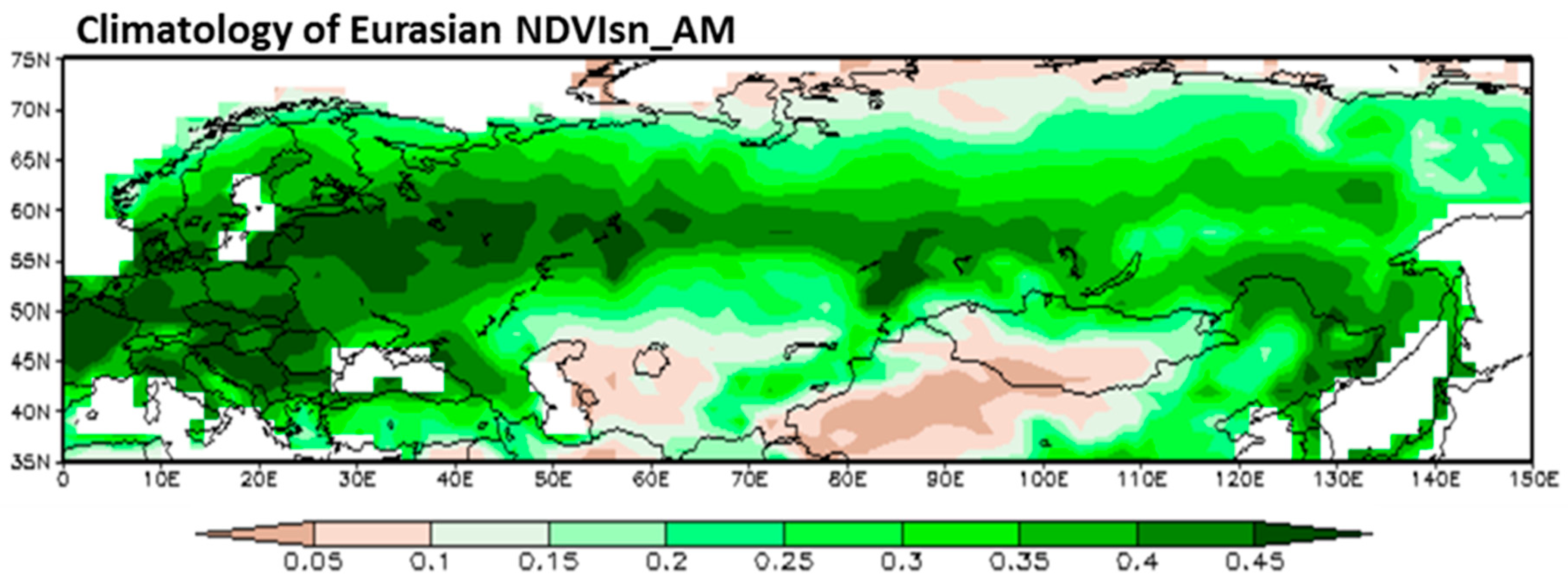
Figure 2.
The first two EOF patterns and corresponding time-series obtained from spring NDVI over Eurasia for the period 1982–2015: (a) the mode of EOF1 in NDVIsn; (b) the time-series of EOF1 in NDVIsn; (c) the mode of EOF2 in NDVIsn; (d) the time-series of EOF2 in NDVIsn; (e) the mode of EOF1 in NDVI3g; (f) the time-series of EOF1 in NDVI3g; (g) the mode of EOF2 in NDVI3g; and (h) the time-series of EOF2 in NDVI3g. The variance explained by each EOF mode is shown on the right corner of figures in the left column.
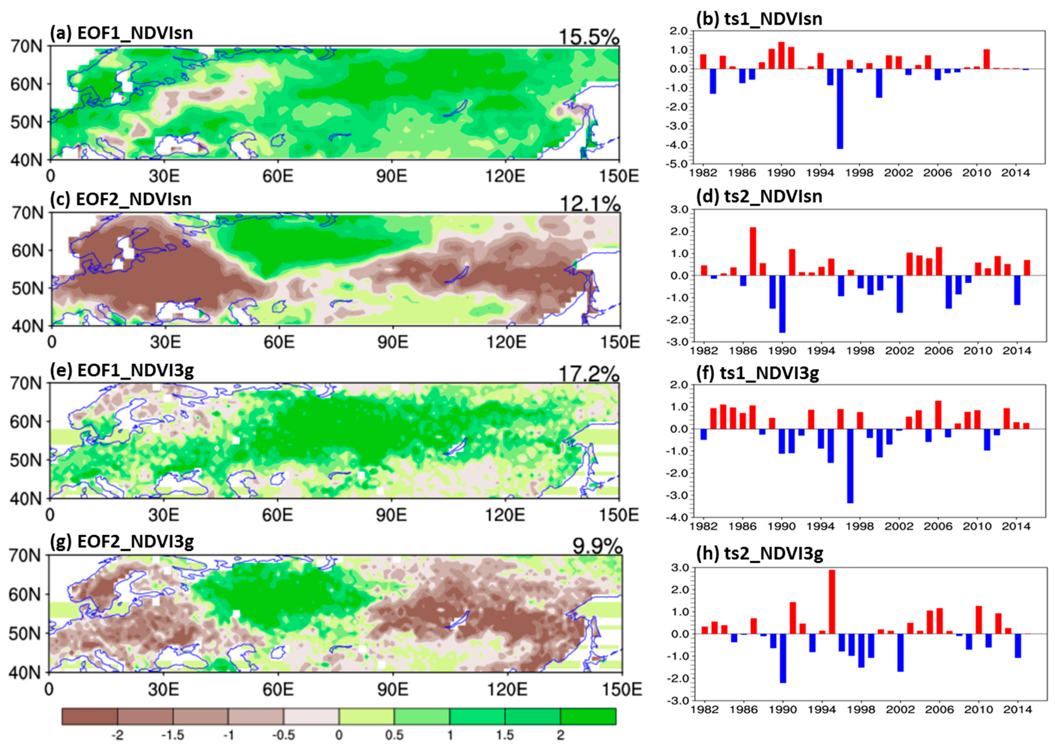
Figure 3.
Spatial patterns of correlation coefficients between spring NDVI and winter climate indices over Eurasia: (a) NDVIsn and Niño4; (b) NDVI3g and Niño4; (c) NDVIsn and Niño3.4; (d) NDVI3g and Niño3.4; (e) NDVIsn and Niño3; (f) NDVI3g and Niño3; (g) NDVIsn and AO; (h) NDVI3g and AO; (i) NDVIsn and NAO, and (j) NDVI3g and NAO. Dotting areas have the correlation coefficient being statistically significant at the 0.1 level (i.e., p < 0.1) estimated by a local Student’s t-test.

Figure 4.
Spatial patterns and time-series of expansion coefficients for the first leading paired mode of winter SST (tropical Pacific) and spring NDVI (Eurasia) for the period 1982 to 2015 via the SVD analysis: (a) the paired mode of SST using NDVIsn; (b) the paired mode of SST using NDVI3g; (c) the paired mode of NDVI using NDVIsn; (d) the paired mode of NDVI using NDVI3g; (e) the time-series of SST (black squares) and NDVI (red dots) using NDVIsn; (f) the time-series of SST (black squares) and NDVI (red dots) using NDVI3g. The time-series amplitudes are normalized based on standard deviation. The variance explained by each SVD is shown on the right corner in (a–d).
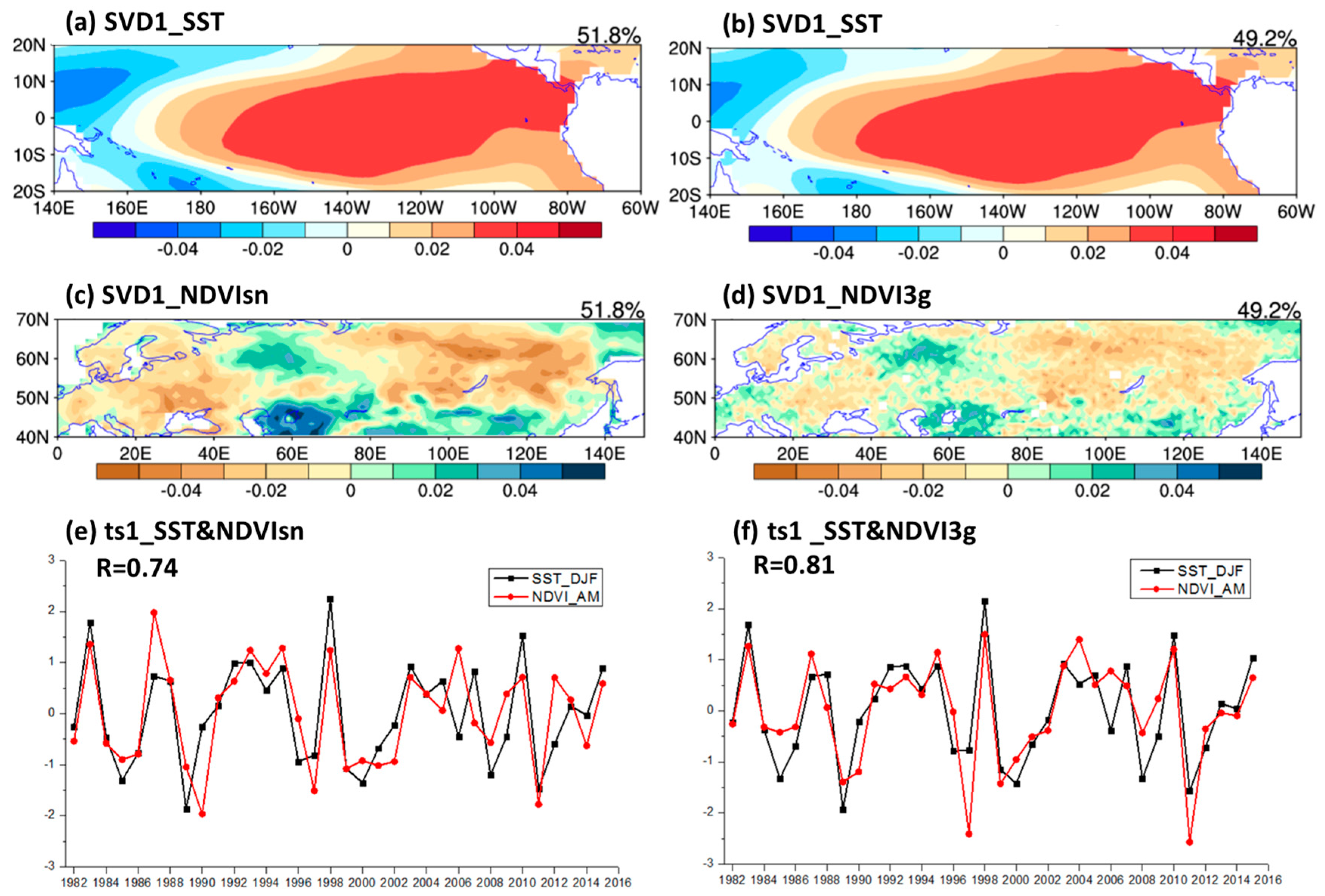
Figure 5.
Spatial patterns and time-series of expansion coefficients for the first leading paired mode of winter SST (tropical Pacific) and ERNDVI for the period 1982 to 2015 via the SVD analysis: (a) the paired mode of SST using NDVIsn; (b) the paired mode of SST using NDVI3g; (c) the paired mode of ERNDVI using NDVIsn; (d) the paired mode of ERNDVI using NDVI3g; (e) the time-series of SST (black squares) and ERNDVI (red dots) using NDVIsn; (f) the time-series of SST (black squares) and ERNDVI (red dots) using NDVI3g. The time-series amplitudes are normalized based on standard deviation. The variance explained by each SVD is shown on the right corner in (a–d).

Figure 6.
Spatial patterns and time-series of expansion coefficients for the first leading paired mode of winter SST (tropical Pacific) and spring surface air temperature (SAT) and precipitation over East Russia for the period 1982 to 2015 via the SVD analysis: (a) the paired mode of SST using SAT; (b) the paired mode of SAT; (c) the paired mode of SST using precipitation; (d) the paired mode of precipitation; (e) the time-series of SST (black squares) and SAT (red dots); (f) the time-series of SST (black squares) and precipitation (red dots). The time-series amplitudes are normalized based on standard deviation. The variance explained by each SVD is shown on the right corner in (a–d).

Figure 7.
Composite anomalies of (a) NDVIsn; (b) SAT (unit: °C) and (c) precipitation (unit: mm/day) during spring in the EP El Niño years over East Russia. Dotting areas have the anomalies being statistically significant at the 0.1 level (i.e., p < 0.1) estimated by a local Student’s t-test.
Figure 7.
Composite anomalies of (a) NDVIsn; (b) SAT (unit: °C) and (c) precipitation (unit: mm/day) during spring in the EP El Niño years over East Russia. Dotting areas have the anomalies being statistically significant at the 0.1 level (i.e., p < 0.1) estimated by a local Student’s t-test.

Figure 8.
Composite anomalies of spring atmospheric circulation (unit: m/s) at (a) 200 hPa; (b) 500 hPa; and (c) 850 hPa in the EP El Niño years. East Russia is in the red box. Shading areas have the anomalies being statistically significant at the 0.1 level (i.e., p < 0.1) estimated by a local Student’s t-test.

Figure 9.
Composite maps of (a) wave activity flux at 200 hPa and (c) geopotential height anomalies at 200 hPa during spring in the EP El Niño years. Composite anomalies of (b) wind at 200 hPa and (d) geopotential height at 200 hPa during spring in the low-value BBR years. Shading areas in (a) and (b), and dotted regions in (c) and (d) have the anomalies being statistically significant at the 0.1 level (i.e., p < 0.1) estimated by a local Student’s t-test.

Figure 10.
(a) composite anomalies of spring rainfall (unit: mm/day) over the Bay of Bengal in the EP El Niño years; (b) changes in the Bay of Bengal rainfall (BBR) (black squares) and Niño3 (red dots) index for the period 1982 to 2015. The dotted regions in (a) have the rainfall anomalies being statistically significant at the 0.1 level (i.e., p < 0.1) estimated by a local Student’s t-test.
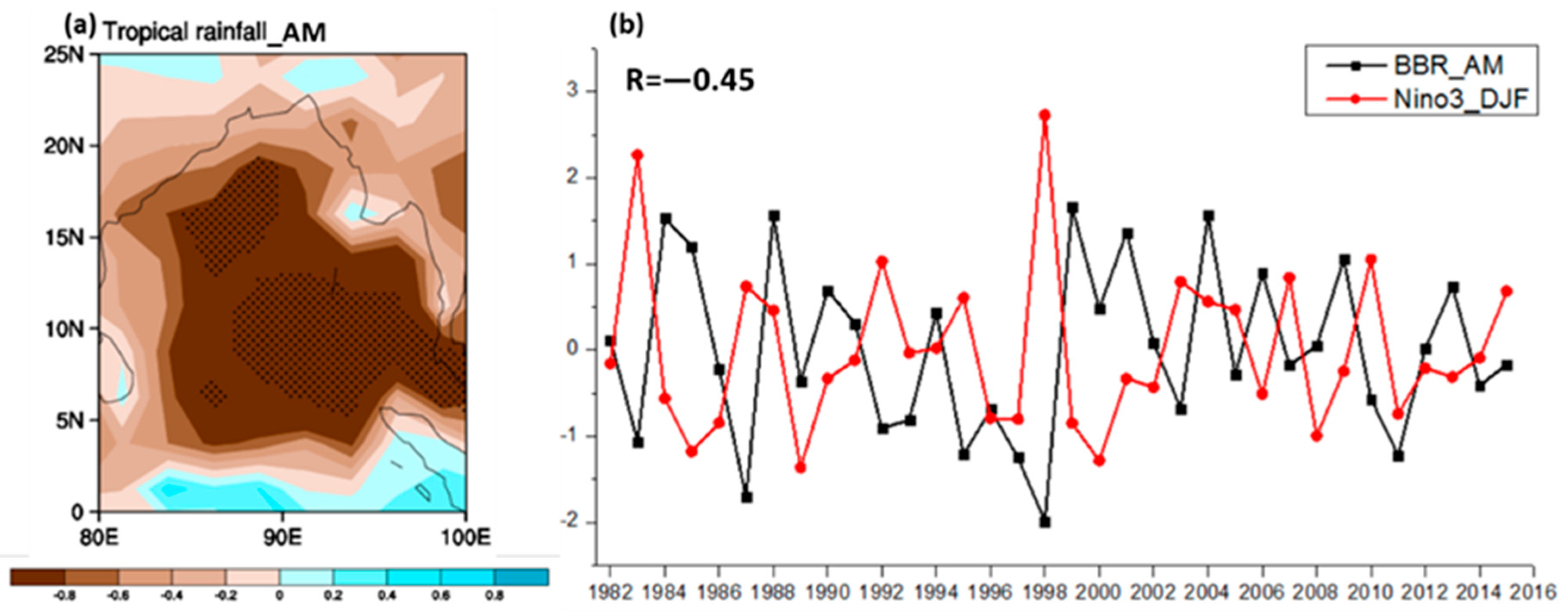
Figure 11.
Schematic diagram of possible physical processes for the teleconnection relationship between EP El Niño and spring ERNDVI.
Figure 11.
Schematic diagram of possible physical processes for the teleconnection relationship between EP El Niño and spring ERNDVI.


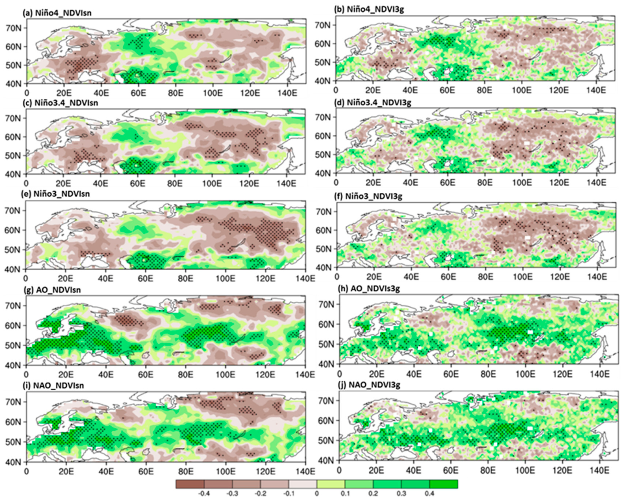
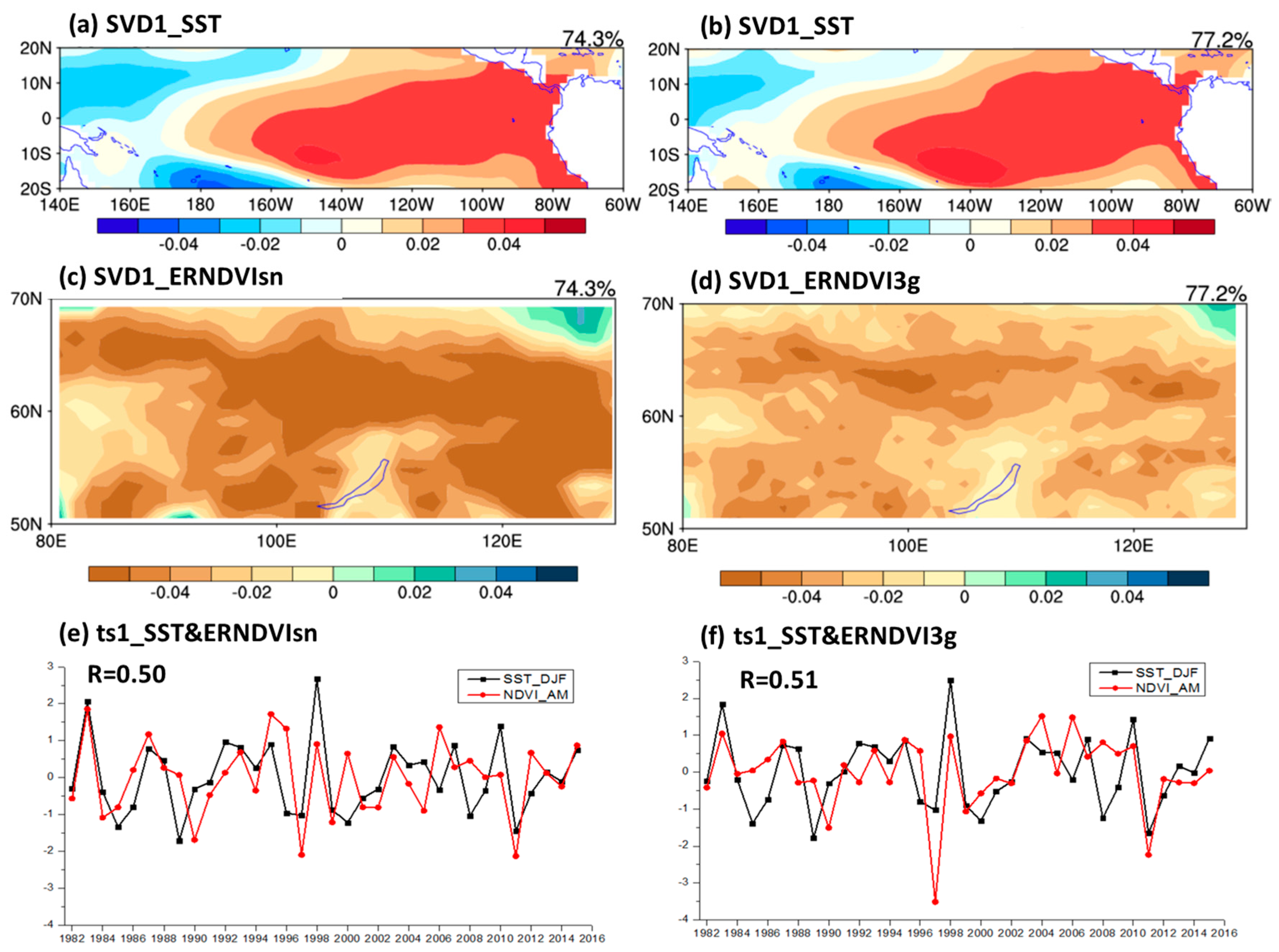
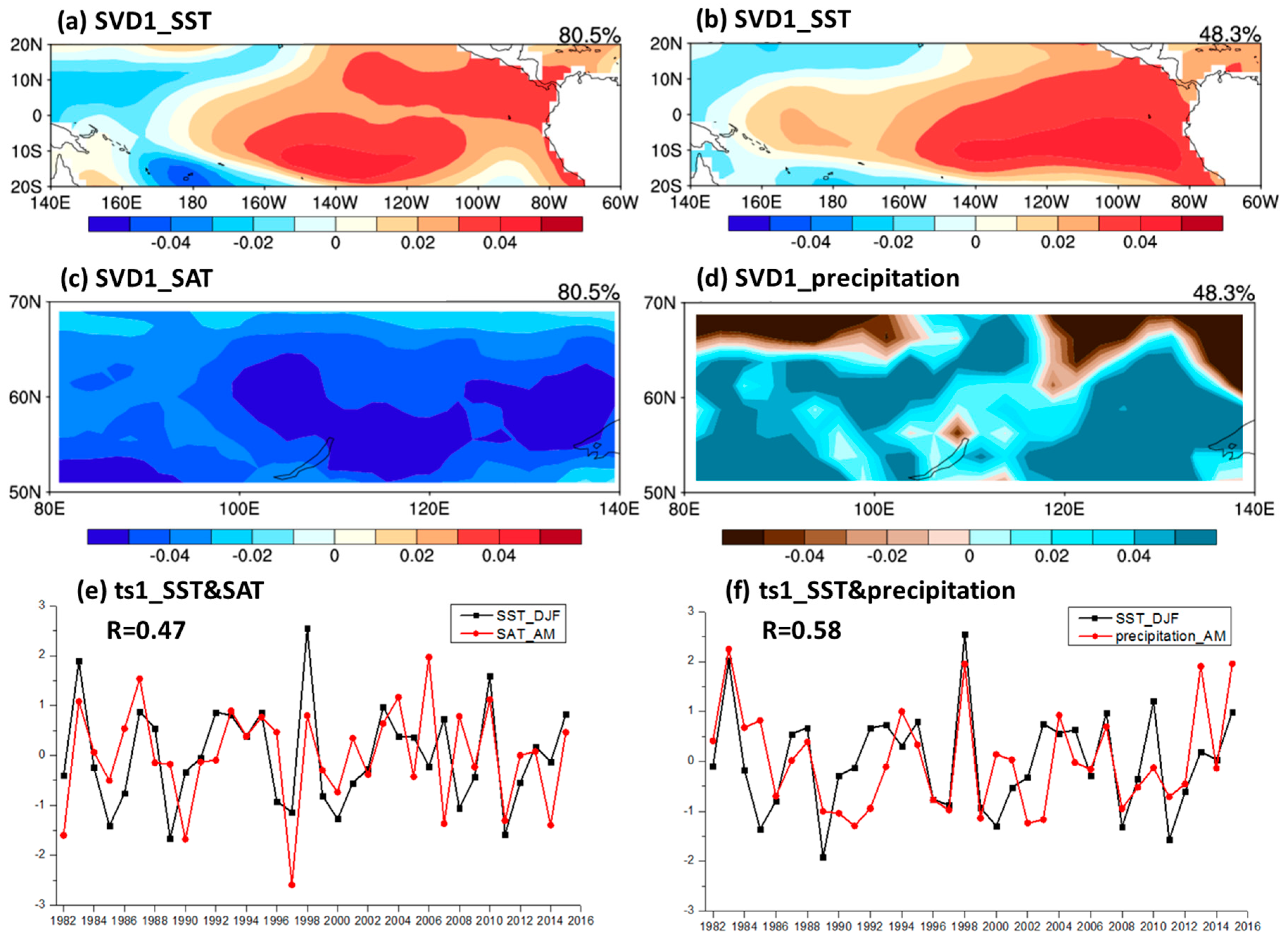
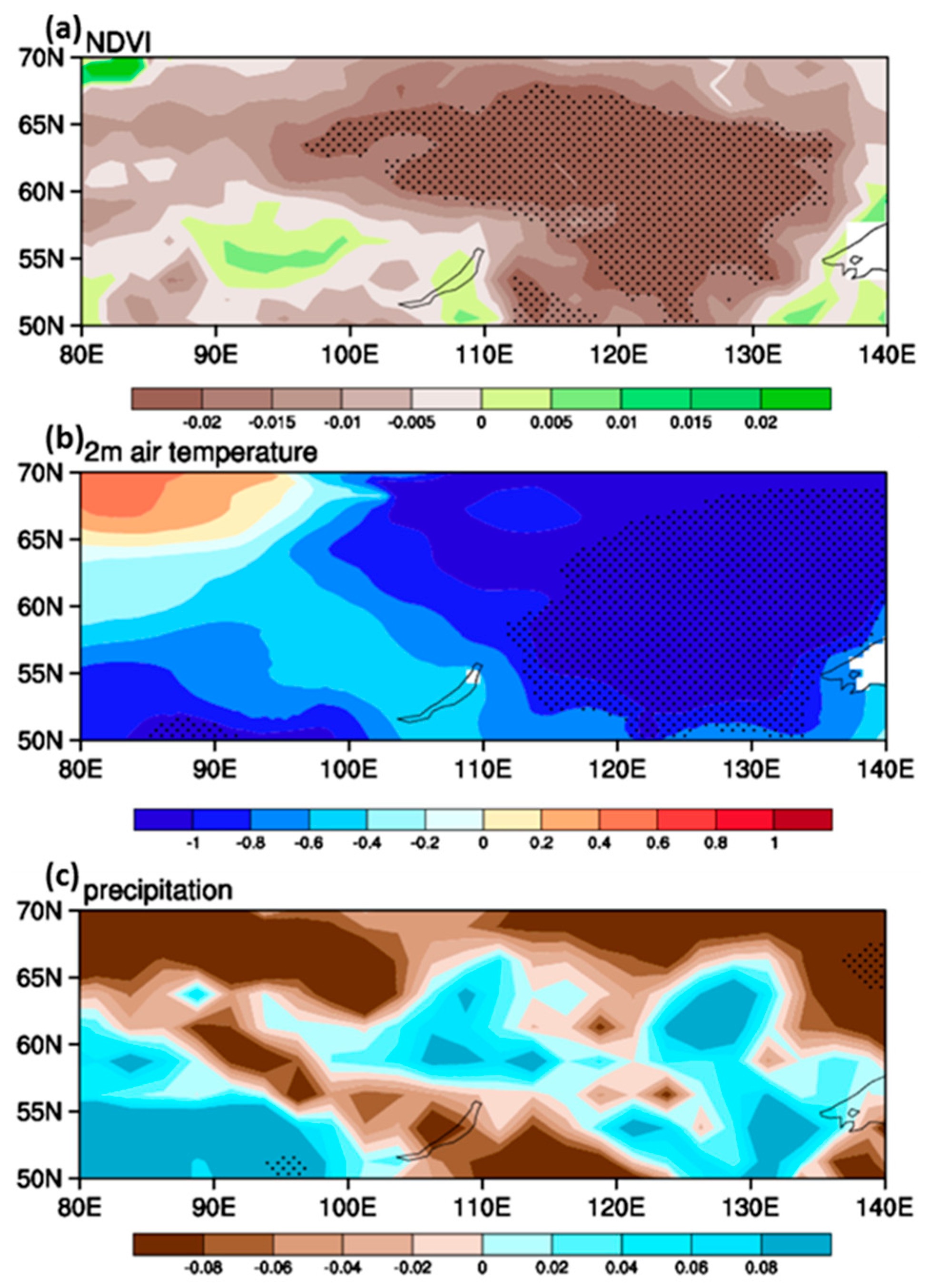
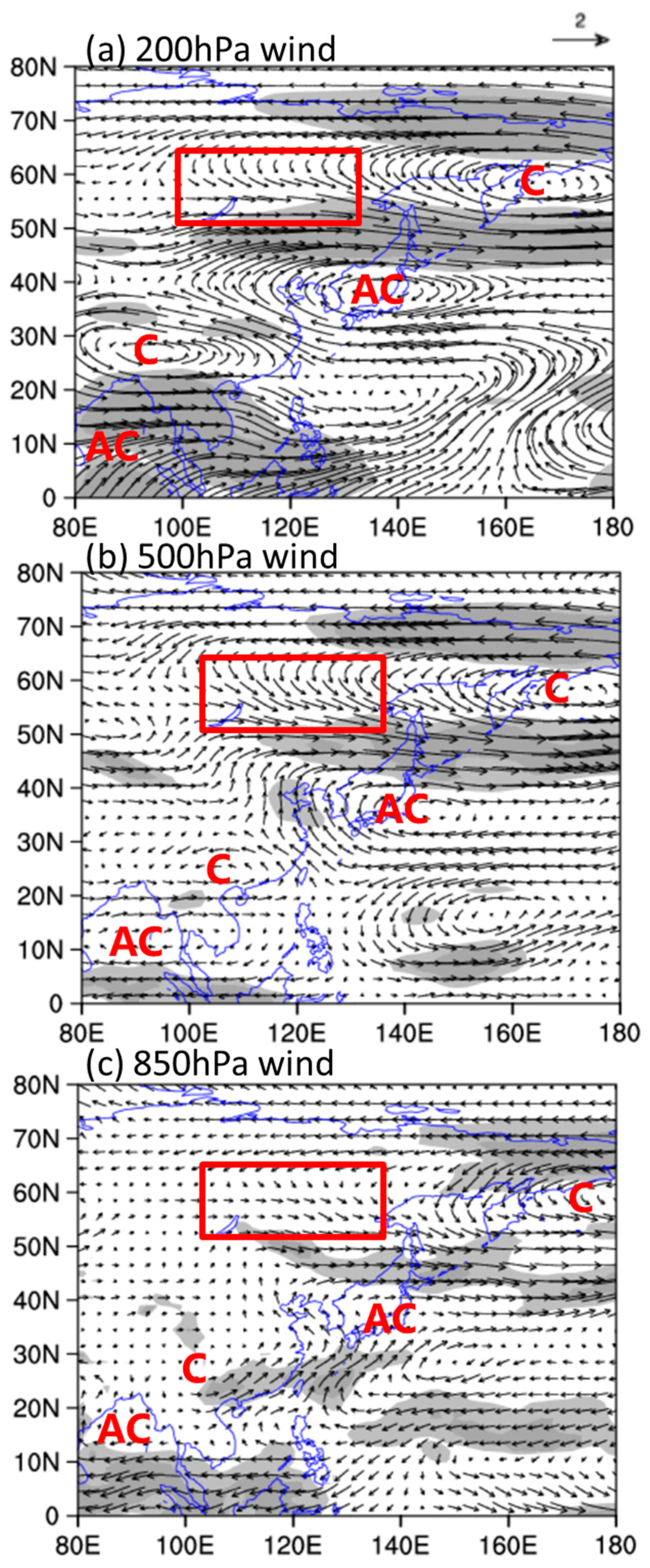
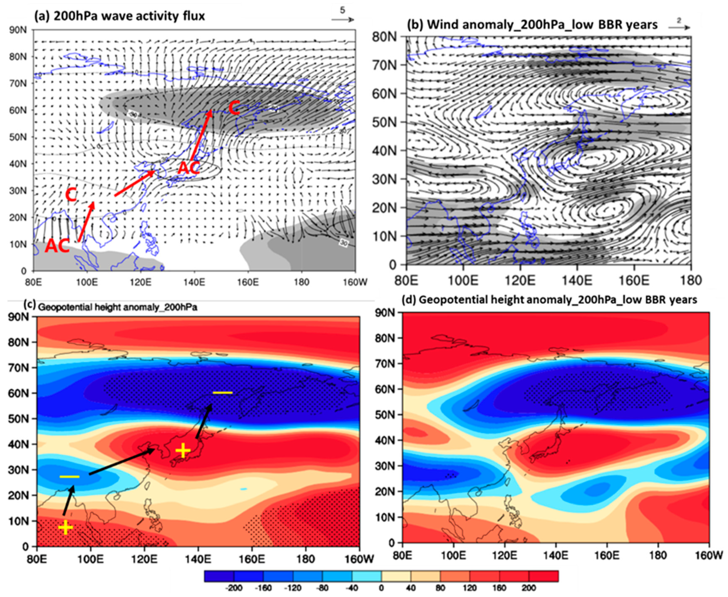
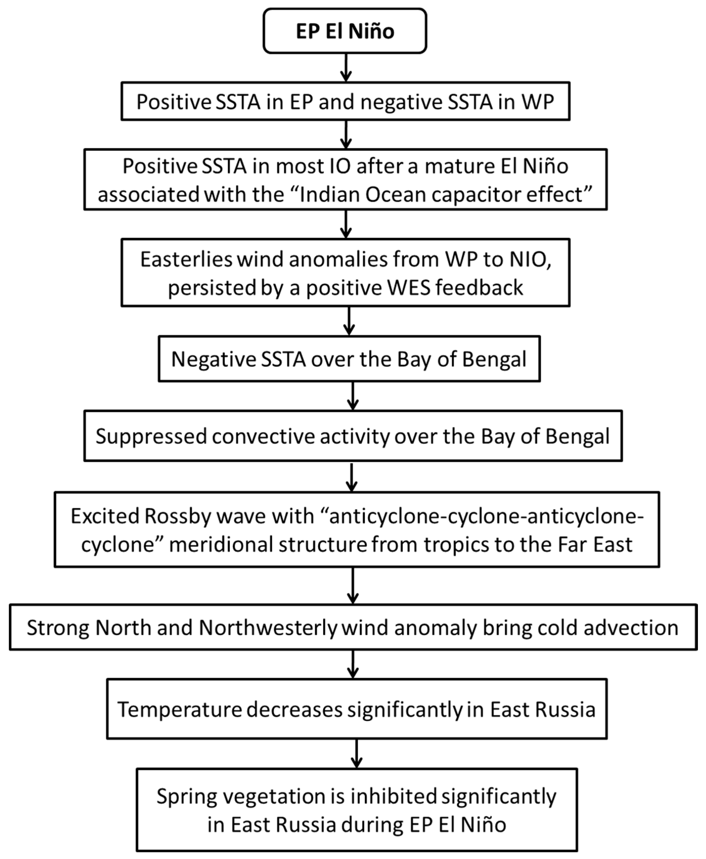
Table 1.
Description of GIMMS and STAR NDVI datasets used in the study.
| Dataset | Provider | Sensor | Temporal Span | Spatial Resolution | Compositing |
|---|---|---|---|---|---|
| NDVI3g | GIMMS | AVHRR | 1981–2015 | 1/12 deg | MVC |
| NDVIsn | STAR | AVHRR | 1981–present | 16 km | MVC smoothed |
Table 2.
Correlation coefficients between spring NDVI and various winter climate indices.
| Indices | NDVIsn_ts1 | NDVIsn_ts2 | NDVI3g_ts1 | NDVI3g_ts2 |
|---|---|---|---|---|
| Niño1+2 | −0.21 | −0.04 | −0.14 | −0.07 |
| Niño3 | −0.19 | −0.22 * | −0.07 | −0.24 * |
| Niño3.4 | −0.12 | −0.29 † | −0.05 | −0.30 † |
| Niño4 | 0.01 | −0.30 † | 0.01 | −0.31 † |
| BEST | −0.20 | −0.24 * | −0.14 | −0.21 |
| NAO | 0.40 ‡ | 0.20 | 0.39 ‡ | 0.23 * |
| AO | 0.51 ‡ | 0.27 * | 0.40 ‡ | 0.36 ‡ |
The correlation values with “*”, “†”, and “‡” are statistically significant at the 0.2 (p < 0.2), 0.1 (p < 0.1) and 0.05 (p < 0.05) level, respectively, estimated by a local Student’s t-test.
Table 3.
Correlation coefficients between the first leading SVD time-series (SST and NDVI) and various winter climate indices based on the two NDVI datasets.
Table 3.
Correlation coefficients between the first leading SVD time-series (SST and NDVI) and various winter climate indices based on the two NDVI datasets.
| Time-series | Niño3 | Niño4 | Niño3.4 | Niño1+2 | NAO | AO |
|---|---|---|---|---|---|---|
| SST_NDVIsn | 0.97 * | 0.82 | 0.97 | 0.86 | / | / |
| NDVI_NDVIsn | 0.51 * | 0.31 | 0.45 | 0.50 | −0.01 | −0.15 |
| SST_NDVI3g | 0.94 * | 0.83 | 0.94 | 0.79 | / | / |
| NDVI_NDVI3g | 0.43 * | 0.28 | 0.38 | 0.40 | −0.27 | −0.37 |
The column with “*” has the most influence in spring ERNDVI.
© 2017 by the authors. Licensee MDPI, Basel, Switzerland. This article is an open access article distributed under the terms and conditions of the Creative Commons Attribution (CC BY) license (http://creativecommons.org/licenses/by/4.0/).
Share and Cite
MDPI and ACS Style
Li, J.; Fan, K.; Zhou, L. Satellite Observations of El Niño Impacts on Eurasian Spring Vegetation Greenness during the Period 1982–2015. Remote Sens. 2017, 9, 628. https://doi.org/10.3390/rs9070628
AMA Style
Li J, Fan K, Zhou L. Satellite Observations of El Niño Impacts on Eurasian Spring Vegetation Greenness during the Period 1982–2015. Remote Sensing. 2017; 9(7):628. https://doi.org/10.3390/rs9070628
Chicago/Turabian StyleLi, Jing, Ke Fan, and Liming Zhou. 2017. "Satellite Observations of El Niño Impacts on Eurasian Spring Vegetation Greenness during the Period 1982–2015" Remote Sensing 9, no. 7: 628. https://doi.org/10.3390/rs9070628
Note that from the first issue of 2016, this journal uses article numbers instead of page numbers. See further details here.