
On-Ground Retracking to Correct Distorted Waveform in Spaceborne Global Navigation Satellite System-Reflectometry


1
School of Electronic and Information Engineering, Beihang University, Beijing 100191, China
2
Earth Observation Researth Group, Institu d’Estudis Espacials de Catalunya (ICE-CSIC/IEEC), 08191 Barcelona, Spain
*
Author to whom correspondence should be addressed.
Remote Sens. 2017, 9(7), 643; https://doi.org/10.3390/rs9070643
Submission received: 7 May 2017
/
Revised: 10 June 2017
/
Accepted: 17 June 2017
/
Published: 22 June 2017
(This article belongs to the Section Ocean Remote Sensing)
Abstract
:Spaceborne Global Navigation Satellite System-Reflectometry (GNSS-R) has been the research focus of Earth observation because of its unique advantages; however, there are still many challenges to be resolved. The reduction of the impact of the satellite motion on the GNSS-R waveform is the one of key technologies for spaceborne GNSS-R. The proposed delay retracking methods in existing literatures require too many instrument resources and too much priori information to refresh correlation window on each coherent integration time period. This paper aims to propose an on-ground alternative in which less frequency tracking refresh on board is needed. The model of dynamic delay waveform, which is expressed as the convolution of the pure waveform and the point spread function, are described. Based on this, the new methodology, which utilizes the least squares fitting to make the residual error between the dynamic model and measured waveform minimum, is employed to reconstruct the pure waveform. The validity of proposed method is verified using UK-DMC, UK-TDS-1 and simulated data. Moreover, the performances of sea surface height and wind speed retrieval using retracked and non-retracked waveforms are compared. The results show that (1) the MSEs between aligned and retracked waveform reduce to 0.026 and 0.044 from 0.110 and 0.156 between aligned and non-retracked waveform with the TRP of 1 s and 3 s for UK-DMC data, and for UK-TDS-1 data, the MSEs decrease from 161.02 and 227.34 to 70.10 and 61.80; (2) the standard deviation of sea surface height using retracked waveform is lower 5 times than the one using non-retracked waveform; (3) the retracked waveform could lead to a better measurement performance in wind speed retrieval. Finally, the relationship between the performance of retracking and Signal-to-Noise Ratio (SNR) is analyzed. The results show that when the SNR of the waveform is lower than 3 dB, the retrieval accuracies rapidly become worse.
1. Introduction
Global Navigation Satellite System-Reflectometry (GNSS-R) which was proposed by Martin-Neira et al. in 1993 [1] has been used to retrieve sea wind speed and significant wave height (SWH). The spaceborne GNSS-R is especially attractive because of its low power-cost, low mass and high spatial-temporal resolution. S. T. Lowe [2] presented the first spaceborne observation of Global Positioning System (GPS) signals reflected from the Earth’s surface, which opened the gates for spaceborne GNSS-R research. First spaceborne retrieval of wind speed was reported by S. T. Gleason [3] who used UK-DMC data to validate the feasibility of retrieving wind speed using spaceborne GNSS-R. The new spaceborne mission, UK-TechDemoSat-1 of the Surrey Satellite Technology Ltd (SSTL) in Guildford of England [4], has been providing more spaceborne GNSS-R data, and the first retrieval of wind speed were presented in [5]. CYGNSS mission of NASA launched in December of 2016 aims to resolve the genesis and rapid intensification phase of the tropical cyclone lift cycle with sufficient frequency [6]. At present, with the increasing of the available spcaeborne GNSS-R data, current studies mainly have focused on developing retrieval approaches or models of wind speed [5,7,8,9,10], sea surface height [11], soil moisture [12,13], sea ice [14,15,16]. To improve the spatial resolution of the observation, some approaches, such as Delay-Doppler Map (DDM) inversion [17,18] and stare processing [19] have been proposed.
Delay waveform as the basic observable of GNSS-R, which is obtained by correlating the reflected GNSS signals and local replicas at different delays, could be used to retrieve sea surface height and wind speed. In general, incoherent averaging among a number of single snapshot should be used to reduce the speckle noise. However, the delay difference between direct and reflected GNSS signals changes rapidly with the motion of the GNSS and LEO satellites [20]. This change should be compensated on each snapshot to avoid the distortion of measured waveform and improve the retrieval performance. The procedure of the compensation is called as tracking. Both GNSS and LEO satellite parameters including height, moving direction and elevation angle are first considered to estimate the delay difference changes (DDC) [21]. The impact of Doppler compensation was accounted for and demonstrated using UK-DMC [22]. A delay tracking method was proposed by H. Park [23] for altimetry by assigning the specular point index of each snapshot on each coherent integration time period. However, a high tracking refresh rate may require too many instrument resources or too much data to be uploaded from the ground station [23]. To reduce the refresh rate above, one way is to decrease the requirement of tracking error and retrieval performance; and the other is to incoherently average each waveform samples on-ground, but needs all waveform samples to be downloaded to the ground station.
This paper focuses on an on-ground retracking method to recovery the waveform from the distorted one which is caused because of the low tracking refresh rate on board. Proposed method aims to use post-processing to replace the compensation on each coherent integration time period on-board to reduce the requirement of too many instrument and much data to be uploaded from the ground station. The simulation scenarios and models used in this paper are presented in Section 2. Section 3 briefly reviews the speckle noise statistics and the incoherent averaging which could significantly mitigate the influence of the speckle noise on the waveform. Section 4 describes the waveform distortion caused by the time-varying observation geometry of GNSS-R. In Section 5, the sensitivity of Arrival Time of Leading Edge (AToLE) to sea surface height and Peak Waveform(PW), Leading Edge Slope (LES), Trailing Edge Slope (TES) to wind speed are analyzed. The detail of the methodology is described in Section 6. The validation of the method using real UK-DMC, UK-TDS-1 and simulated data is given in Section 7. The comparison of sea surface height and wind speed retrieval using retracked and non-retracked waveform are shown in Section 8. Final, the conclusion is addressed in Section 9.
2. Simulation Scenario and Models
To analyze delay retracking, it is necessary to develop a spaceborne GNSS-R simulator which includes scattering scenario, GNSS-R scattering model and noise models.
2.1. Scenario
In simulation, a local coordinate system as shown in Figure 1 is developed, in which (1) the coordinate origin is at earth’s core; (2) the YOZ plane is in the incident plane; (3) Z axis has the same direction with the normal of the tangent plane of the specular point; (4) and it is assumed that earth, the orbits of GNSS and LEO satellite are circular. The gain pattern of receiver antenna is assumed as Gaussian function as
where and are the maximum gain and 3 dB beam width, respectively; is the included angle between the direction of receiver antenna pointing and scattering unit . The parameters of simulation scenario are shown in Table 1.
2.2. GNSS-R Scattering Models
The GNSS-R scattering model was derived by Zavorotny et al. [24] using bistatic equation model and Kirchhoff Approximation as
where and are the transmitted power and transmitter gain, which are 26.8 W and 12.1 dB for GPS L1 signal; is the wavelength of the signal, which is 0.19 m for GPS L1 signal; and are the delay and Doppler frequency for signals reflected by scattering unit ; is the local carrier frequency; is the autocorrelation function of the code; ; and are the distance from LEO and GNSS satellite to the scattering unit ; is the Fresnel reflection coefficient; is the scattering vector ; is the probability density function of ocean surface slopes, and is assumed as two-dimensional Gaussian function. The variances of are obtained by Elfouhaily spectrum [25] which is relative to wind speed.
2.3. Noise Models
The delay waveform is impacted by two noises which are thermal and speckle noise as
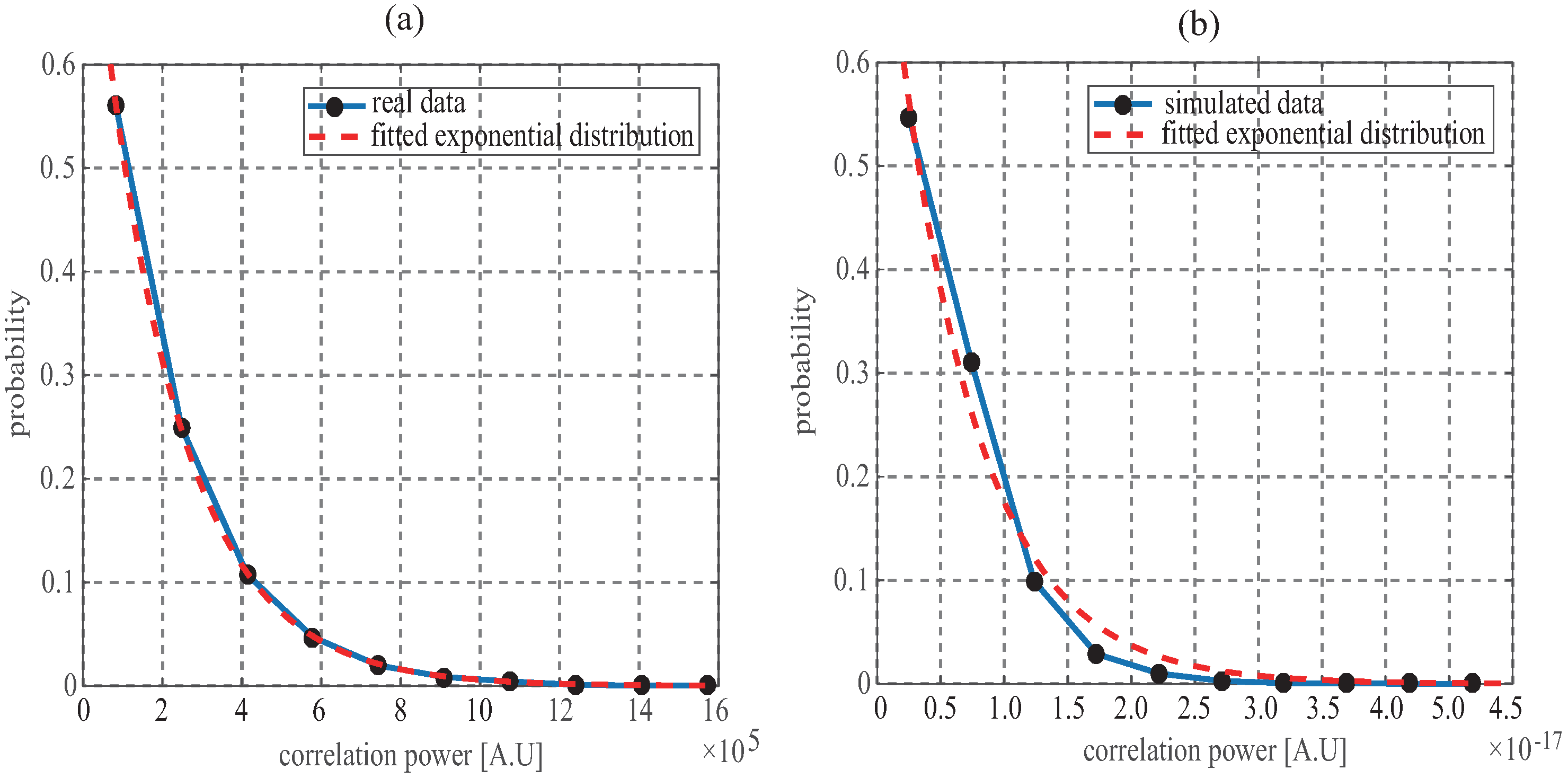
where is speckle noise which caused by coherence of scattered signals from multiple scattering units. Many models of speckle noise have been proposed. In [17], speckled measurements were simulated assuming that the amplitude of the reflected signals follows a Rice distribution. In Synthetic Aperture Radar (SAR) system, the K-distribution [26] or unit-mean exponential distribution [27] were used to model the speckle noise. For GNSS-R, S. Gleason et al. [28] performed a detailed analysis on signal fading statistics using the UK-DMC data and found that the scattered GNSS signals from ocean followed the exponential probability. Figure 2a which is the distribution of scattered GNSS signals for UK-TDS-1 presents the same phenomenon that a exponential function could well fit the distribution of real data received from spaceborne configuration. Overall, in this paper, the speckle noise is assumed as an unit-mean exponential distribution. Figure 2b shows the distribution of simulated GNSS-R correlation power using scattering and speckle noise models above, from which it is clear that the simulated results also approximately is subject to the exponential distribution. In in-phase and quadrature branch, the thermal noises are assumed to be Gaussian distribution as
where is the noise power. takes chi-squared distribution . Therefore, the additive noise in Equation (3) could be modeled as
3. Speckle Noise vs. Incoherent Averaging
As described above, in scattered GNSS signals from rough surface, there is an importance noise called as speckle noise which occurs as a result of constructive and destructive interference between the signals scattered by different scattering unit in the glistening zone. F. T. Ulaby et al. [29] discussed the statistic of speckle noise from rough surface scattering theory, and found that the probability distribution of the single snapshot took the form of an exponential as well as the discussion in [28] for UK-DMC data. The same distribution could be obtained using UK-TDS-1 data as shown in Figure 2. The significant approach to reduce the impact of this noise on the waveform is to incoherently average a number of consecutive single snapshot as
where is the number of incoherent averaging. The standard deviation of the peak of the measured waveform could be estimated to quantify the influence of the speckle noise. According to the results of F. T. Ulaby and S. Gleason, the standard deviation of the incoherently averaged waveform decreases as a function of the number of incoherent averaging as
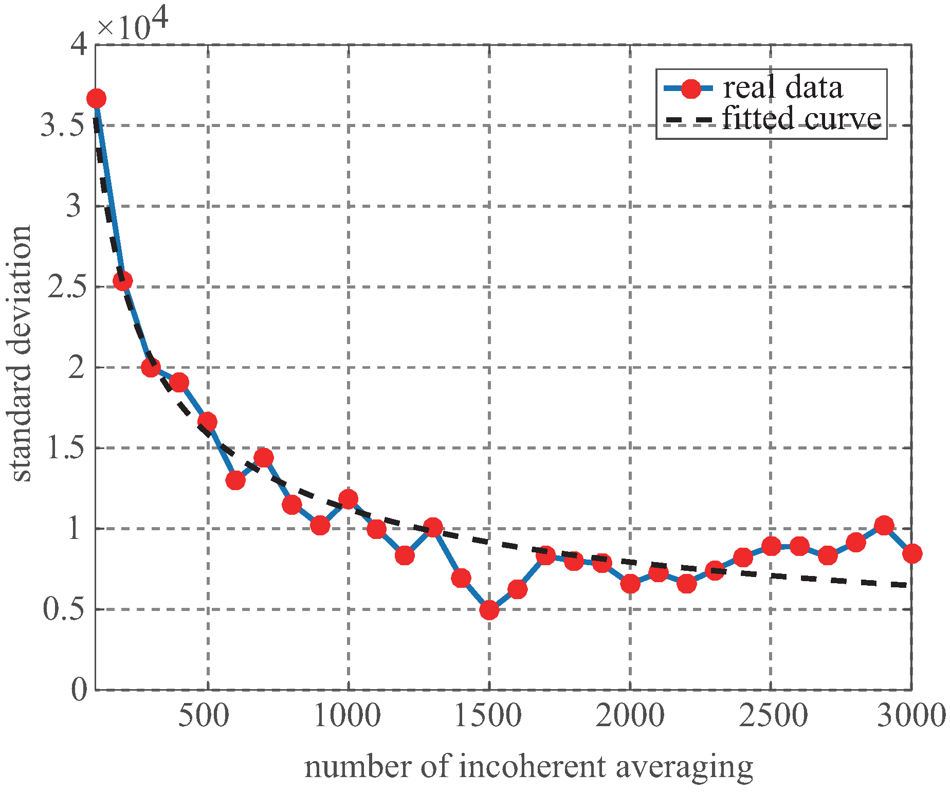
where is the standard deviation of the single snapshot. Figure 3 presents the reducing tendency of the standard deviation as the number of incoherent averaging increases, in which the dotted line is the fitted using Equation (8). When the number of the incoherent averaging is larger than 1000 which is usually considered as the incoherent time for GNSS-R, the trend of decreasing becomes slow, however, it is still necessary to adopt the incoherent averaging number over 1000 to further improve the measurement accuracy. As given in [30], regardless of C/A and P(Y) code for altimetry, the achieved height precisions for the incoherent averaging number of 1000 is lower than the ones for the incoherent averaging number of 60,000.
4. Influence of Dynamic on Waveform
To reduce the influence of thermal and speckle noise, delay waveform samples are incoherently averaged. Because of the high dynamics of LEO and GNSS satellite, the snapshot moves each other when incoherent averaging is performed as
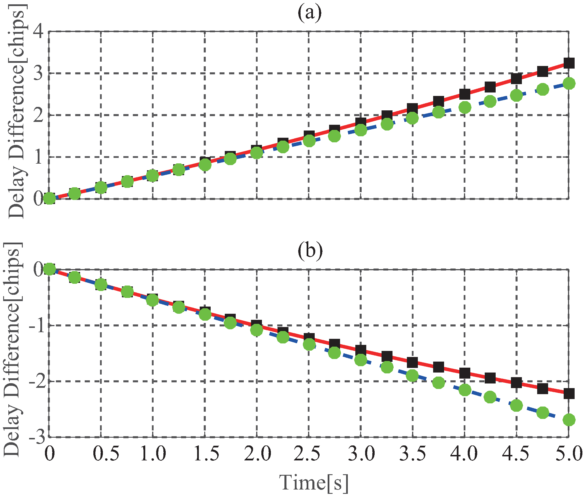
where is the delay difference between the and first waveform sample, which is determined by the geometry configuration of GNSS and LEO satellites, such as the hight, elevation, moving direction of satellite. The red solid lines in Figure 4 give the simulated results of the change of the delay difference between direct and reflected signals, in which the delay difference changes show an approximately linear relationship over the time in a short period of time. The blue dotted lines in Figure 4 show the linear curves with the slope of 0.54 and −0.52 for Figure 4a,b, from which it is found that the disagreements between the delay difference and the linear curves increase over the time. This behavior illustrates that in fact the delay difference is not linear as shown in the following where Delay Difference Change Rate (DDCR) is time-varying. Figure 5 shows the delay waveform with the tracking refresh period of 1 ms, 1 s, 3 s, from which it is seen that if the waveform samples are not aligned when incoherent averaging is conducted, incoherent averaging causes a distortion of averaged waveform, moreover, the longer the tracking refresh period is, the more serious the distortion is. This distortion results in a degradation of the retrieval performance as analyzed in [21] in which the results show that the performance of spaceborne GNSS-R altimeter is seriously degraded without a proper alignment of the waveform samples. As proposed in [22], the ideal case is that the correlation window is refreshed on each coherent integration period (e.g., 1 ms). However, a high refresh rate requires too many instrument resources and too much data to be uploaded from the ground station. Therefore, it is necessary to find an alternative with the less tracking refresh rate.
4.1. Delay Change Rate
In [21,22], the dependence of the DDCR on the moving direction of LEO and GNSS satellites, the height and the incidence angle of LEO satellite are simulated, however, the analytical expression as the function of the navigation parameters, such as Doppler frequency or pseudo range rate, is not presented. Here, a relationship linking DDCR with the Doppler frequency difference between reflected and direct signals is given as (the detail derivation could be found in the Appendix A).
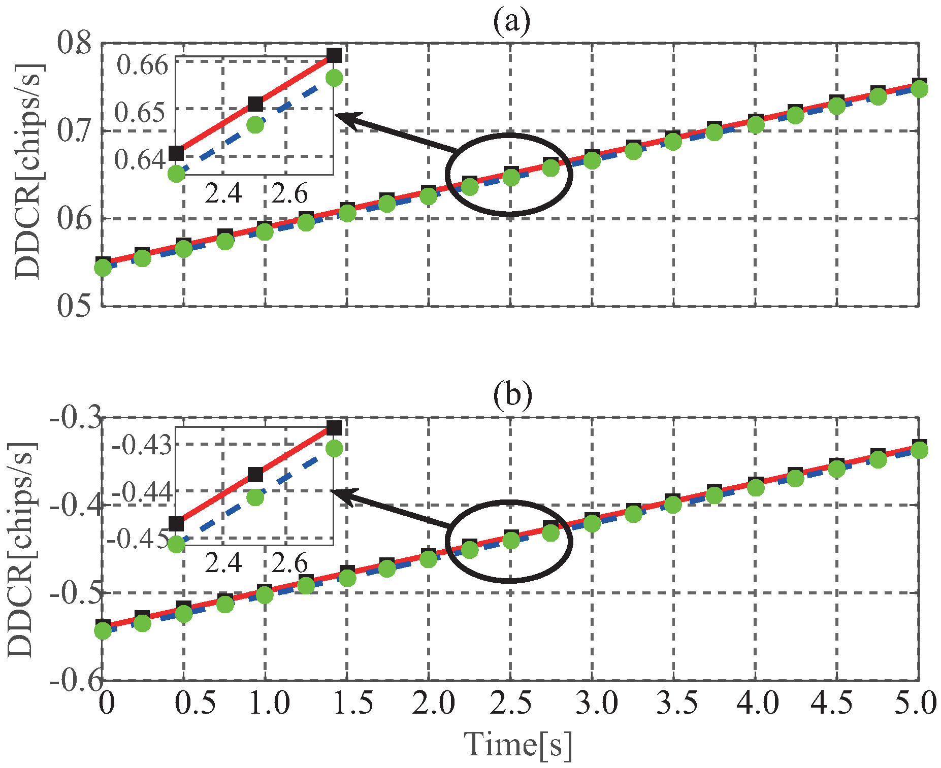
where is the wavelength of the signal, which is 0.19 m for GPS L1; is the Doppler frequency difference of reflected and direct signals at the time t. Figure 6 gives the tendency of the simulated and computed DCR with the changing of the time, in which the simulated DDCR has ignored difference with the computed one using Equation (10). Furthermore, it is noticeable that the DDCR shows time-varying behavior which illustrates that the delay difference between direct and reflected signals is nonlinear function as the time as presented in Figure 4 and mentioned above.
5. Influence on Feature Parameter
To describe the delay waveform, some features are defined such as Arrival Time of Leading Edge(AToLE), Peak Waveform (PW), Leading Edge Slope (LES), and Trailing Edge Slope (TES) as
is the specular delay from maximum first the derivation on the waveform leading edge [31]. Among them, AToLE could be used to determine sea surface height, and the others are relative to wind speed as described in [7]. In [21], it has been pointed that the change of waveform results in the bias errors in the estimation of the specular delay AToLE. In this section, their influence on retrieving sea surface height using AToLE and wind speed using PW, LES and TES are further analyzed. To compare quantitatively, the sensitivity of the feature parameters to sea surface height or wind speed are defined as
where is the incidence angle; and p represents sea surface height h or wind speed W; f represents the function of feature parameter as sea surface height or wind speed.
5.1. Sea Surface Height
In [32], a retrieval model of sea surface height was proposed as
where c is lightspeed; and are ranges from LEO and GNSS satellite to the predicted specular on the Earth’s ellipsoid; is the propagation distance of GNSS signals from GNSS satellite to the specular point, and then to LEO satellite. According to the expression above, the sensitivity of AToLE to sea surface height is
From the equation above, it could be seen that the sensitivity of AToLE to sea surface height is only relative to the incident angle. In other word, it means that if the each waveform samples are not tracked on each coherent integration time period or non-aligned waveform are not be retracked on ground, it only results in the bias error in the estimation of AToLE, has no impact on the sensitivity of retrieving sea surface height.
5.2. Wind Speed
The model of retrieving wind speed is not like the one of measuring sea surface height and is usually not obtained through theoretical derivation. The frequently-used method is to develop the empirical relationship using measured feature parameters and in situ wind speed. From existing literature [8,9], those relationships usually are not linear so that the sensitivity of feature parameters to wind speed are dependent to feature parameters. The simulated results of the sensitivity of PW, LES and TES to wind speed are given as Figure 7. From the figure, it is clear that as wind speed increases, the sensitivity of three feature parameters to wind speed become weak. Moreover, the change of the observation geometry of GNSS-R not only causes the estimation error of feature parameters as mentioned above, but also weakens the sensitivity of feature parameters to wind speed. This reduction becomes serious with the increasing of the TRP.
6. Methodology of Retracking
Equation (9) could be written as
where is the pure waveform; is the change of delay difference between adjacent waveform samples; ⊗ is the convolution operator; is the Dirac function; and is called as the point spread function (PSF). By measured waveform and PSF, the pure waveform could be estimated using the deconvolution, such as in [17,18] where the constrained least squares (CLS) and the truncated singular value decomposition (TSVD) were used to reconstruct scattering coefficient () from Delay-Doppler Map (DDM), respectively. In fact, many reconstruction methods have been proposed to solve deconvolution in image processing, however, unfortunately, either those methods are unsuitable to solve the problem with the existing of the large noise level, or their performance have dependence on the choice of the method parameter. The parameter p of (TSVD) in [17] and of CLS in [18] are key point to control the reconstruction results. In this paper, Least Square Matching (LSM) is used to estimated the pure waveform as
where represents the measured waveform. This method aims to find proper wind speed and delay to minimize the root mean square error between averaged waveform and modeled one by Equation (9) or (18) minimum. It is noted that this method has the same procedure with the processing of retrieving wind speed using Least Square Matching (LSM), the only difference is that this method considered the impact of the time-varying geometry configuration of GNSS-R. The estimated is relative to the delay used in altimeter. As known, the Z-V model is time- and resource-consuming, hence, it is difficult to be used in fast processing. The alternative approach is to find an analytic function to replace Model (2) as
where are fitted parameters; and
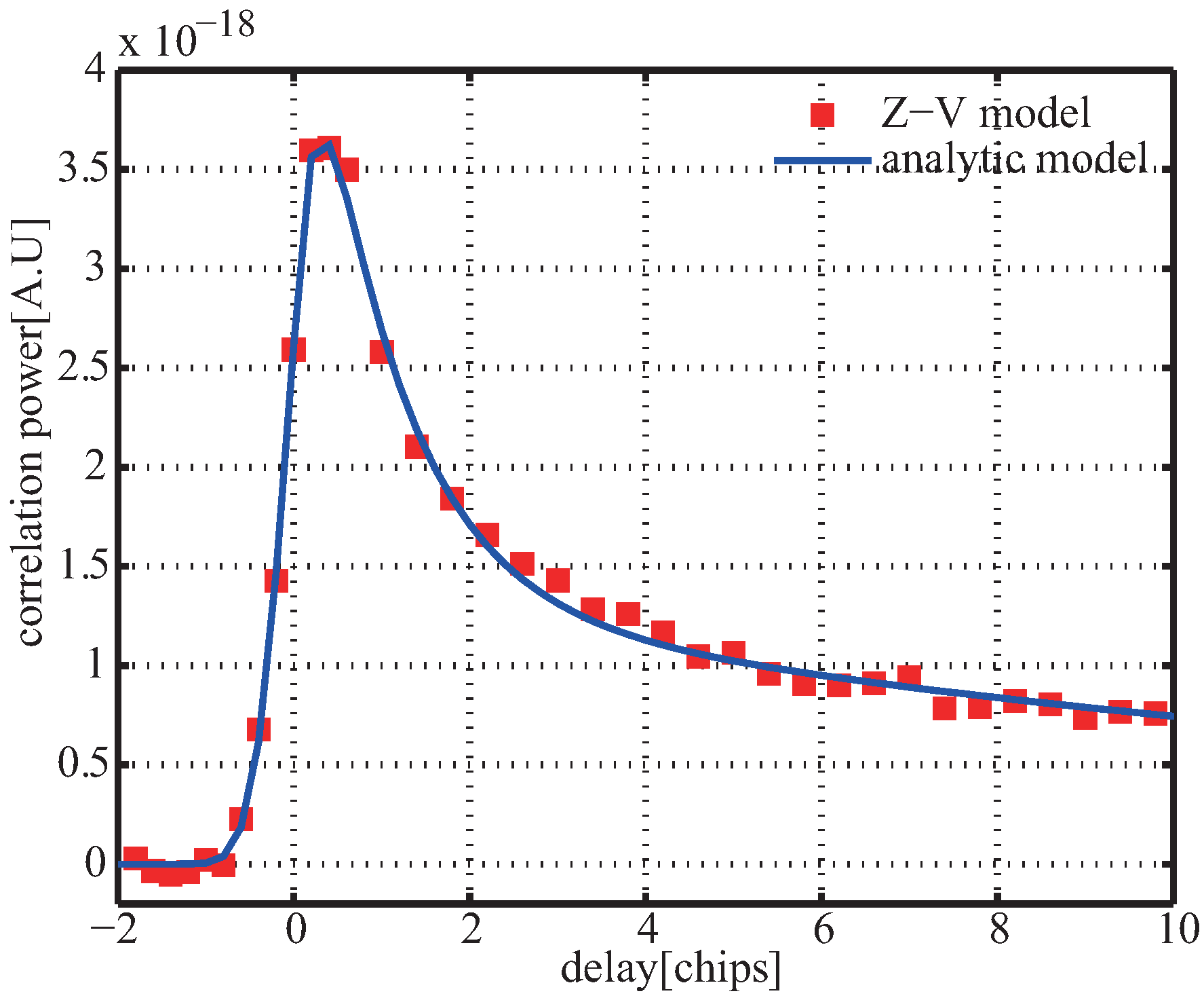
Figure 8 presents simulated delay waveform and the fitted result using analytic Function (20), from which it is seen that by finding proper , the delay waveform could be replaced well by (20). Therefore, Equation (19) is changed to
The retracking processing of distorted waveform on-ground is outlined in Figure 9, in which the detailed steps are implemented as follow:
- using estimated Doppler difference between direct and reflected signals to produce the DDCR and PSF;
- developing model of the distorted waveform using convolution Equation (18) and the initial coefficients of the Model (20);
- fitting the distorted model above with the measured waveform using nonlinear least square to obtain the optimal coefficients of (20);
- reconstructing the pure waveform using the Model (20) and the estimated coefficients above.
7. Results and Discussion
In this section, the proposed method is validated using the United Kingdom’s Disaster Monitoring Constellation (UK-DMC) satellite data, United Kingdom’s Technology Demonstration Satellite-1 (UK-TDS-1) data over the ocean surface and the simulated data.
7.1. Validation Using UK-DMC Data
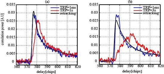
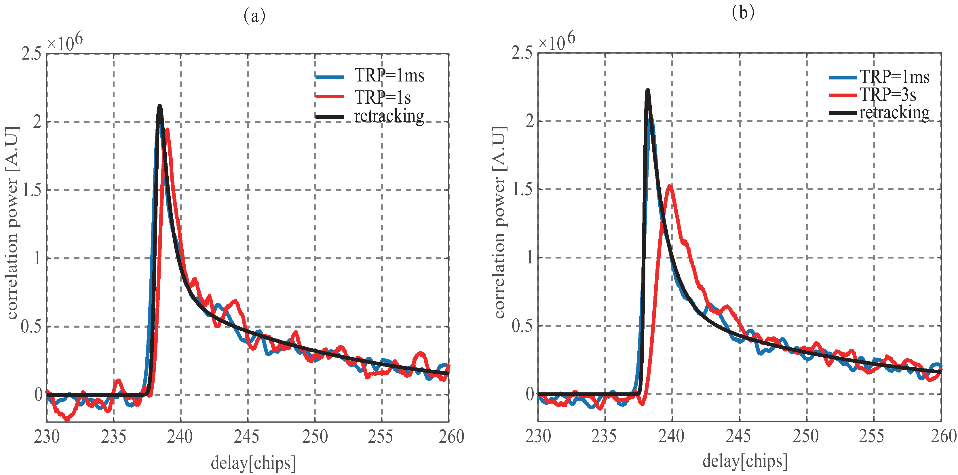
To drive the development and exploitation of GNSS-R on-board, an experimental GPS reflectometry receiver was equipped with UK-DMC satellite [33]. The UK-DMC satellite was launched into a 680 km sun synchronous orbit as part of the disaster monitoring constellation in October 2003 and the first successful data collection was on 22 October 2005 [20]. Here, the data collected on 16 November 2004 over the ocean surface is used to verify the proposed approach. The red lines in Figure 10a,b are the averaged waveform with the tracking refresh period of 1 s and 3 s, respectively. It is clear that compared to the waveform with the tracking refresh period of 1 ms, which are shown by the blue curves in Figure 10, those waveforms without proper delay compensation are distorted. The deformation is more serious when tracking refresh period is longer as mentioned above. In [22], according to the observation geometry at the time of data collection, the delay difference change rate is computed as 5.97 chips/s, therefore, in this paper is 0.00597. The retracked waveform using Equation (21) are displayed by the block curves in Figure 10 from which it is noted that the deformed waveforms are recovered well. Compared the mean squared errors (MSEs) of 0.110 and 0.156 between the non-aligned waveform with the refresh period of 1 s and 3 s and the aligned waveform, respectively, the MSEs between retracked and aligned waveform reduce to 0.026 and 0.044. In addition, comparing to the results of retracking for the distorted waveform with the TPR of 1 s and 3 s, it is could be seen that the retracking performance for the waveform of 1 s is better than the one of 3 s. The one reason is that the waveform of 3 s have more serious deformation than the one of 1 s; the other is that, as shown in Figure 4, the longer TPR results in the larger disagreement of delay difference change when in Model (18) is assumed as the constant.
7.2. Validation Using UK-TDS-1 Data
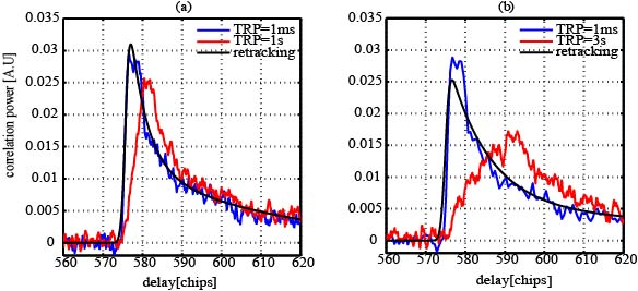
Following the success of the UK-DMC mission, the UK-TDS-1 satellite which embarked on a new generation GNSS-R receiver SGR-ReSI was launched on 8 July 2014 [4]. The UK-TDS-1 data products range from Level 0 (raw intermediate frequency samples) to Level 2 (DDM). The Level 2 products have been incoherently averaged on-board. This paper uses the Level 0 data of the RD16 which could be downloaded free from the website http://www.merrrbys.org/atlas/atlas. By Equation (10), the delay difference change rate could be estimated as 0.78 chip/s. As shown in Figure 11, compared to the distortion of delay waveform in Figure 10, the less delay difference change rate results in the lower distortion of delay waveform. The recovered waveforms have higher similarity degree with the aligned waveform than the one before retracking. The MSEs reduce to 70.10 and 61.80 from 161.02 and 227.34 for the waveform with the TRP of 1 s and 3 s. Although for the UK-TDS-1 data selected to demonstrate retracking approach here, the retracking performance of the waveform with the TRP of 3 s is better than the one with the TRP of 1 s, it still should be noted that the waveform with the shorter TRP have better retracking performance, which will be further proofed in the following section.
7.3. Validation Using Simulation
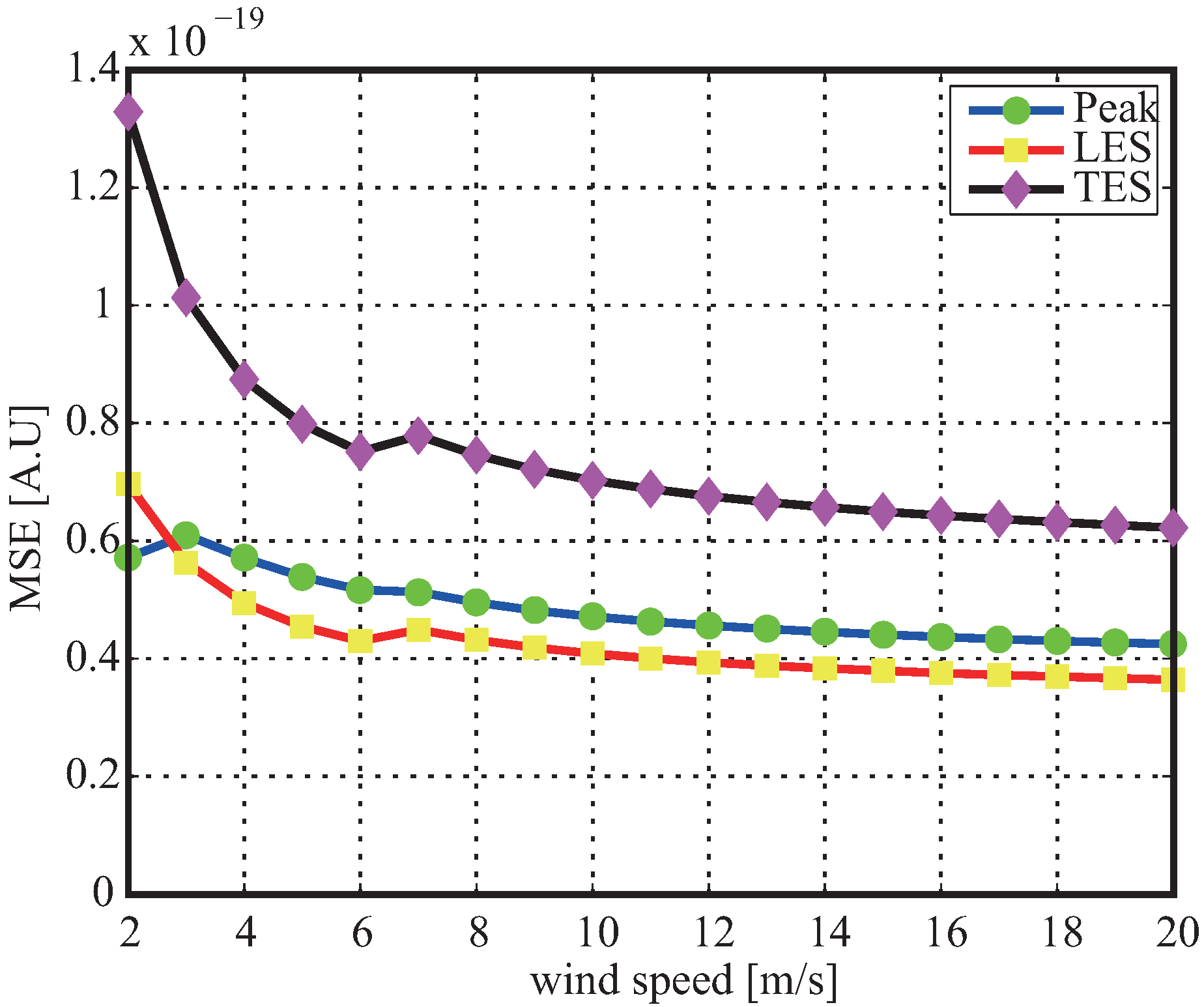
The comparisons of the sensitivity of PW, LES and TES of retracked and non-retracked waveform to wind speed are presented in Figure 7. From the figure, it is clear that the PW, LES and TES of retracked waveform have more sensitive to wind speed than the ones of non-retracked waveform. In addition, retracking method proposed above could recover PW and LES better than TES. To explore the reason, the mean square errors of leading edge, peak and trailing edge between Z-V waveform and the corresponding analytical Model (20) are computed. The results are given in Figure 12 which shows that the fitting error of the TES is much larger than the ones of the PW and LES. In other word, the larger fitting error of the TES causes the poorer retracking result compared to the ones of the PW and LES.
7.4. Comparison with CLS and TSVD Result
As mentioned above, many approaches could be use to solve deconvelution, however, because of the large noise level, most of methods could not show well reconstruction results. In this subsection, the comparison of recovery performance between the proposed approach in this paper and the ones in [17,18] is performed. Table 2 presents the comparison result, in which compared to the other two approaches, the proposed method has the best recovery performance. It is worth noting that the recovery results of the CLS and TSVD have importance dependence on the parameter and p. The same phenomenons that adjusting the parameter controls the influence of the noise could be found in Figures 4 and 5 of of [18]. Moreover, differing form the waveforms reconstructed using the CLS and TSVD, the one obtained by the proposed approach is smooth so that the feature parameters of the waveform could be directly estimated from the recovered waveform without any other procedures such as the linear fit to estimate LES and TES of the waveform in [8].
7.5. Influence of DCR Accuracy
In fact, the model exists with errors because of the inaccuracy DDCR estimation which is caused by the errors of the measured position and velocity of LEO and GNSS satellite. In this section, the impact of the DDCR error on the retracking performance is discussed. Figure 13 shows the change of the MSE between the retracked waveform and the aligned one over the DDCR. From the figure, it is clear that the accuracy of the DDCR has important influence on the retracking result. Compared to the retracking for the waveform with the TPR of 3 s, retracking the waveform of 1 s requires lower DDCR accuracy. In addition, from Figure 13b, it could be also seen that for the UK-TDS-1 data the waveform of 1 s has better retracking result than the one of 3 s besides DDCR being 0.75 chips/s. According to the analysis above, retrakcing approach proposed above could recover the distorted waveform, however, it is needed to improve the TPR on-board to obtain higher retracking performance. In other words, the TPR on-board should be reasonably selected considering the retracking and final retrieval accuracy.
8. Retrieval Performance
To compare the retrieval performance of sea surface height and wind speed using retracked and non-retracked waveform, the following simulation steps are implemented as:
- generating randomly 1000 sets of wind speed, incident angle, the moving direction of LEO and GNSS satellites as the input parameters of the models in Section 2;
- using scattering scenario and models in Section 2 to produce 1000 delay waveform corrupted by the noises and the dynamic of GNSS-R geometry;
- retracking above delay waveforms to obtain pure ones through proposed methods in Section 6 and estimating the retracked and non-retracked waveforms’ features defined by (11)∼(14);
- developing retrieval approaches and evaluating the root mean square error (RMSE) of sea surface height and wind speed measured using retracked and non-retracked waveforms.
8.1. Sea Surface Height
The retrieval performance of sea surface height could be characterized by the standard deviation of the estimated height. The delays of retracked and non-retracked waveform are obtained through determining the AToLE. The standard deviation of sea surface height error could be expressed as
where is the standard derivation of the AToLE. Table 3 gives the comparison of the standard deviation of the estimated height using retracked and non-retracked waveform, from which it is seen that (1) when the correlation windows are refreshed on each coherent integration time period, the best retrieval performance with the standard derivation of 4.71 m is obtained; (2) for the waveform with the TRP of 1 s and 3 s, the standard derivation of the estimated delay is 6.19 and 11.49 m, which are improved over 6 and 10 times than the non-retracked waveforms. Moreover, it is also noted that the precision of the estimated height for retracked waveform is decreases as the TRP increasing. Retracking method proposed above significantly improves the precision of the estimated height.
8.2. Wind Speed
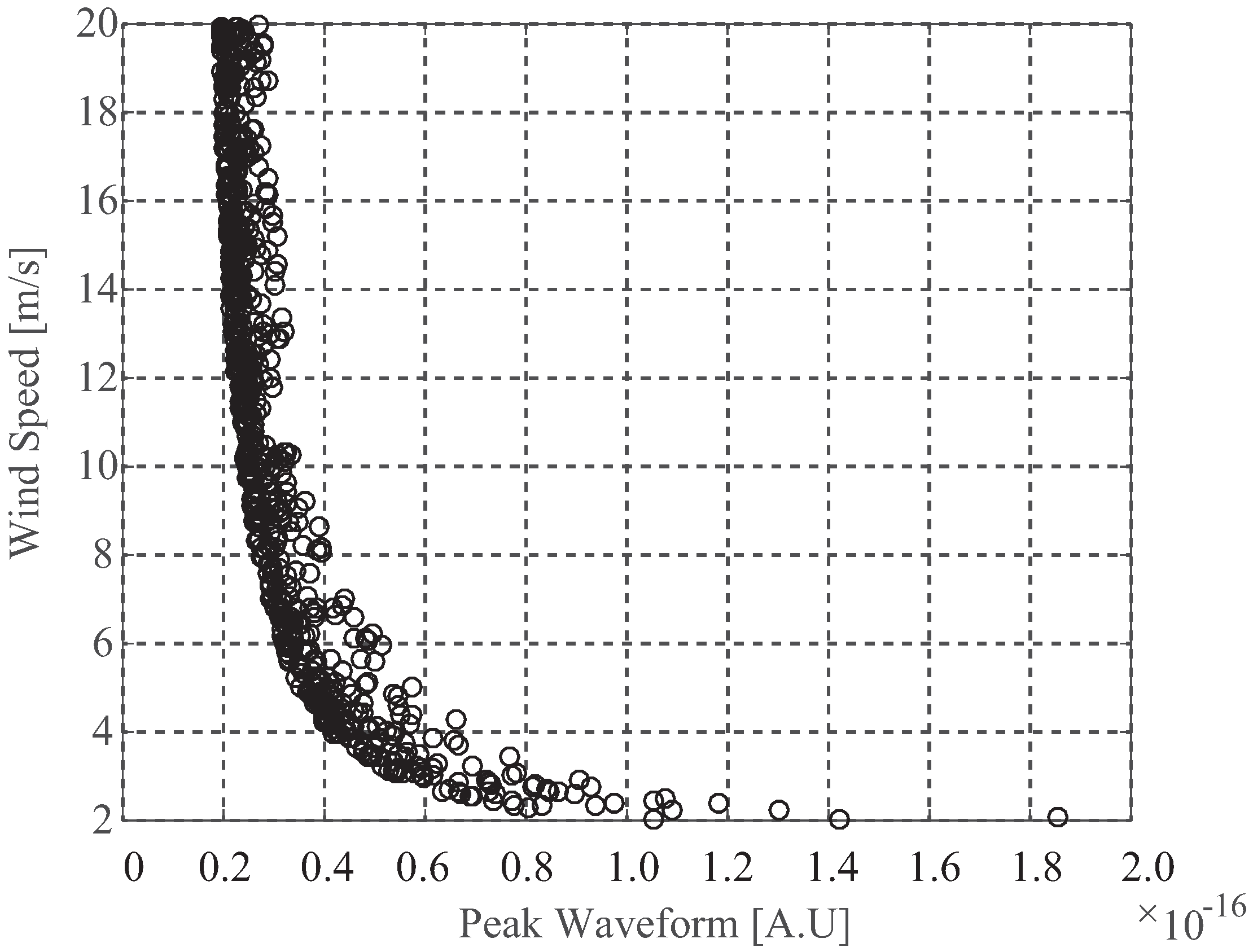
The methods of retrieving wind speed have been proposed using the LES and TES and waveform area by [7,8], which are all to develop empirical mapping function between wind speed and the observable above. As shown in Figure 14, it is clear that wind speed has inversely proportional relationship with PW. In this paper, the analytic links between the wind speed and the observable are replaced by the neural network [34], in which the hidden layer has three neurons, neuron functions in the hidden layer is Sigmoid and in the output layer is purelin as
To compare the performance of the single and multiple-parameter observation, two cases are adopted.
- case 1: the single observable of the delay waveform, such as PW, is the input of neural network;
- case 2: the three observable are all considered as the input of the neural network.
When developing retrieval models of wind speed, 1000 sets of simulated data are divided two groups. One group are considered as training set and the other as test set.
Table 4 gives comparisons of retrieved wind speed using retracked and non-retracked waveform, from which it is summarized that (1) the result that retrieved wind speed using retracked waveforms have better precision than the ones using non-retracked waveforms, which indicates that the proposed retracking method is valid; (2) the less the TRP is, the higher the retrieval results using retracked waveform are, hence, to obtain the better precision of retrieved wind speed, higher tracking refresh rata on-board is needed; (3) combining all observable waveforms to retrieve wind speed could significantly improve measurement performance, hence, multi-parameters observation which could uses more feature information of the waveform is a trend to improve retrieval precision.
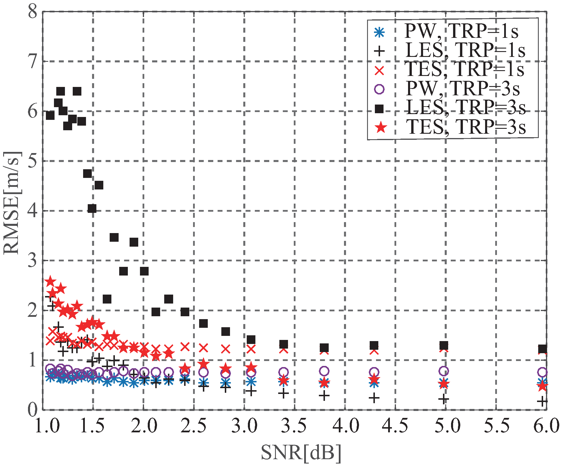
8.3. Performance vs. SNR
The signal-to-noise ratio (SNR) has important influence on the accuracy of GNSS-R techniques. Here, It is needed to analyze the dependence of retracking performance on the SNR. In GNSS-R, the SNR could be defined the scale of processed signal power exceeding the processed noise level as [20]
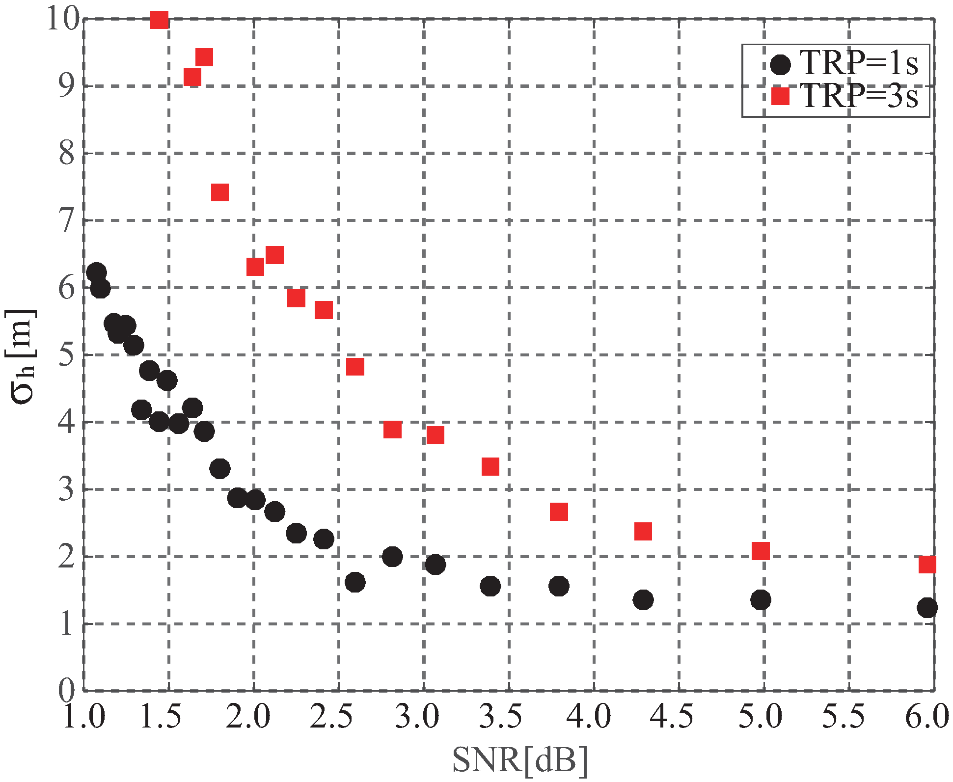
where is the noise floor level which could be computed by averaging all delay waveform points before the first correlation power of the reflected signal. In the paper, the SNR refers in the proportion between the peak waveform and the noise floor, i.e., . Here, the only differentia of simulation steps with the above is that the noise level in Equation (6) is also considered to be random to produce the delay waveform with different SNR. Figure 15 and Figure 16 show the improving tendencies of retrieval performance using retracked waveform as the SNR increases. When the SNR is lower than 3 dB, the retrieval accuracies rapidly become worse. For wind speed, the retrieval performance using peak waveform and leading edge slope are the least and worst affected by the SNR, respectively.
9. Conclusions
This paper proposed a on-ground retracking method to reduce on-board tracking frequency. The sensitivity of the feature parameters of non-retracked waveform to sea surface height and wind speed are discussed. Compared to the aligned waveform, the sensitivity of non-retracked waveform to wind speed is decreasing. The proposed method was verified through real UK-DMC, UK-TDS-1 data and simulation. After retracking non-aligned waveform of UK-DMC, the MSEs between aligned and retracked waveform reduced 0.026 and 0.044 from 0.110 and 0.156 for 1 s and 3 s incoherently averaged waveform, respectively. For UK-TDS-1 data, the MSEs decreased from 161.01 and 227.34 to 70.10 and 61.80. Moreover, the sensitivity of retracked waveform to wind speed was improved. The retrieval performance of sea surface height and wind speed were analyzed. The results showed that the best performance was obtained using aligned waveform; for sea height retrieval, the standard deviation of the estimated height using retracked waveform could reduce over 5 and 10 times than using non-retracked waveform with the TPR of 1 s and 3 s, respectively; the RMES of retrieved wind speed using retracked waveform significantly are reduced compared to the non-retracked waveform. Finally, the dependence of retrieval accuracies using retracked waveform on the SNR was discussed. It was concluded that when the SNR is lower than 3 dB, the retrieval performance rapidly get worse. Above all, proposed method could be implemented on-ground to reconstruct delay waveform from the one corrupted by the dynamic of LEO and GNSS satellite.
In fact, the most complete GNSS-R observable is two-dimensional Delay-Doppler Map (DDM). As mentioned as in [22], not only the delay , but also Doppler frequency varies with the motion of the LEO and GNSS satellite. Therefore, it is needful to adjust correlation window in delay and Doppler domain on board or to recover the DDM from distorted one. In future, our work will be to develop a two-dimensional motion distortion model of the DDM, and based on this, propose an approach to reconstruct DDM.
Acknowledgments
The authors would like to thank Surrey Satellite Technology Ltd. for providing UK-DMC data in this paper and the reviewers for reviewing to improve the quality of the paper.
Author Contributions
F. W proposed the approach and drafted the manuscript; D. Y put forward the architecture of the paper; W. L processed the spcceborne data; W. Y derived the relationship between the DDCR and the Doppler difference of reflected and direct signals. All of the authors contributed to the result discussion and paper writing.
Conflicts of Interest
The authors declare no conflict of interest.
Appendix A. Derivation of Delay Difference Change Rate
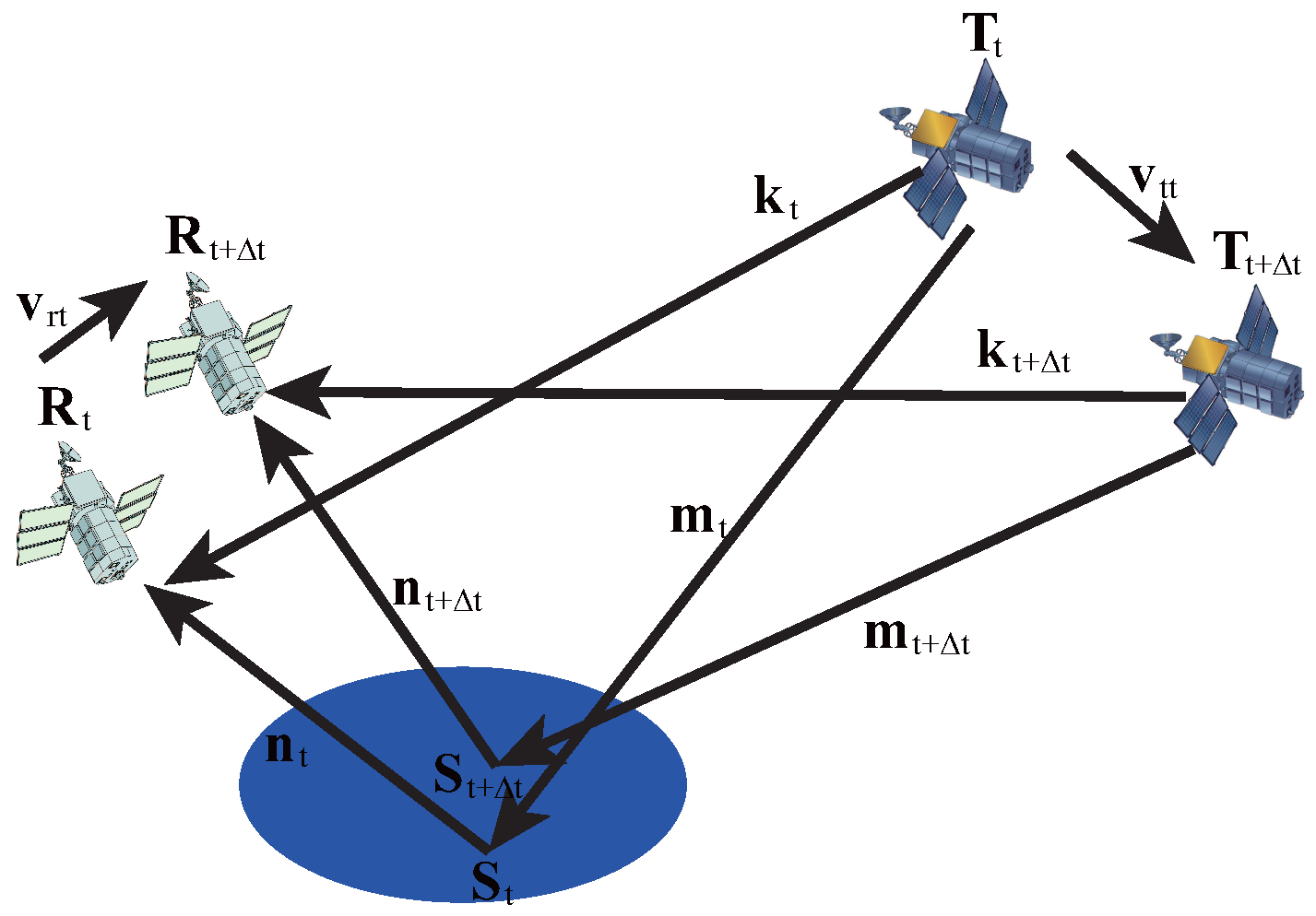
The change of observation geometry during is shows in Figure 16 in which , , , , and are the position at time t and , respectively; and , and , and are the unit vector from GNSS satellite to specular point, from specular point to LEO satellite and from GNSS to LEO satellite at t and , respectively; and are the velocity of LEO and GNSS satellite at t. When is a small value, , , .
Figure A1.
Dynamic observation geometry as LEO and GNSS moving.

The delay of direct and reflected signals at t and are
The DDCR is defined as
The second term of the right is the delay change rate of direct signals and could be simplified as
where is the Doppler frequency of direct signals at t. Similarly, the first term of the right is the delay change rate of reflected signals and could be simplified as
where is the Doppler frequency of reflected signals at t. According to the derivations above, finally, DDCR is the function as the Doppler difference between reflected ans direct signals as
References
- Martin-Neira, M. A passive reflectometry and interferometry system (PARIS): Applocation to ocean altimetry. Ecol. Soc. Am. J. 1993, 17, 331–335. [Google Scholar]
- Lowe, S.; LaBrecque, J.L.; Zuffada, C.; Romans, L.J.; Young, L.E.; Hajj, G.A. First spaceborne observation of an Earth-reflected GPS signal. Radio Sci. 2002, 37, 1–28. [Google Scholar] [CrossRef]
- Gleason, S.T.; Yiping, S.H.S.; Gommenginger, C.; Mackin, S.; Adjrad, M.; Unwin, M. Detection and processing of bistatically reflected GPS signlas from low Earth orbit for the purpose of ocean remote sensing. IEEE Trans. Geosci. Remote Sens. 2005, 43, 1229–1241. [Google Scholar] [CrossRef]
- Unwin, M.; Duncan, S.; Jales, P.; Blunt, P.; Brenchley, M. Implementing GNSS reflectometry in space on the TechDemoSat-1 misson. In Proceedings of the 27th International Technical Meeting of The Satellite Division of the Institute of Navigation, Tampa, FL, USA, 8–12 September 2014. [Google Scholar]
- Foti, G.; Gommenginger, C.; Jales, P.; Unwin, M.; Shaw, A.; Robertson, C.; Rosello, J. Spcaeboren GNSS reflectometry for ocean winds: First results from the UK TechDemoSat-1 mission. Geophys. Res. Lett. 2015, 42, 5435–5441. [Google Scholar] [CrossRef]
- Ruf, C.S.; Gleason, S.; Jelenak, Z.; Katzberg, S.; Ridley, A.; Rose, R.; Scherrer, J.; Zavorotny, V. The CYGNSS nanosatellite constellation hurricane mission. In Proceedings of the 2012 IEEE International Geoscience and Remote Sensing Symposium, Munich, Germany, 22–27 July 2012; pp. 214–216. [Google Scholar]
- Clarizia, M.P.; Ruf, C.S.; Jales, P.; Gommenginger, C. Spaceborne GNSS-R minimum variance wind speed estimator. IEEE Trans. Geosci. Remote Sens. 2014, 52, 6829–6843. [Google Scholar] [CrossRef]
- Clarizia, M.P.; Ruf, C.S. Wind speed retrieval algorithm for the Cyclone Global Navigation Satellite System (CYGNSS) mission. IEEE Trans. Geosci. Remote Sens. 2016, 54, 4419–4432. [Google Scholar] [CrossRef]
- Rodriguez, N.; Garrison, J.L. Generalized linear observables for ocean wind retrieval from calibrated GNSS-R delay-Doppler maps. IEEE Trans. Geosci. Remote Sens. 2016, 54, 1142–1155. [Google Scholar] [CrossRef]
- Soisuvarn, S.; Jelenak, Z.; Said, F.; Chang, P.S.; Egido, A. The GNSS reflectometry response to the ocean surface winds and waves. IEEE J. Sel. Top. Appl. Earth Obs. Remote Sens. 2016, 9, 4678–4699. [Google Scholar] [CrossRef]
- Clarizia, M.P.; Ruf, C.; Cipollini, P.; Zuffada, C. First spaceborne observation of sea surface height using GPS-reflectometry. Geophys. Res. Lett. 2016, 43, 767–774. [Google Scholar]
- Chew, C.; Shah, R.; Zuffada, C.; Hajj, G.; Masters, D.; Mannucci, A. Demonstrating soil moisture remote sensing with observation from the UK TechDemoSat-1 satelllite mission. Geophys. Res. Lett. 2016, 43, 3317–3324. [Google Scholar] [CrossRef]
- Camps, A.; Park, H.; Pablos, M.; Foti, G.; Gommenginger, C.P.; Liu, P.W.; Judge, J. Sensitivity of GNSS-R spaceborne observations to soil miosture and vegetation. IEEE J. Sel. Top. Appl. Earth Obs. Remote Sens. 2016, 9, 4730–4742. [Google Scholar] [CrossRef]
- Hu, C.; Benson, C.; Rizos, C.; Li, Q. Single-pass sub-meter space-based GNSS-R ice altimetry: Results from TDS-1. IEEE J. Sel. Top. Appl. Earth Obs. Remote Sens. 2017. [Google Scholar] [CrossRef]
- Yan, Q.; Huang, W.; Moloney, C. Neural networks based sea ice detection and concentration retrieval from GNSS-R delay-Doppler maps. IEEE J. Sel. Top. Appl. Earth Obs. Remote Sens. 2017. [Google Scholar] [CrossRef]
- Schiavulli, D.; Frappart, F.; Ramillaume, G.; Darrozes, J.; Nunziata, F.; Migliaccio, M. Observing sea/ice transition using radar images generated from TechDemoSat-1 delay Doppler maps. IEEE Geosci. Remote Sens. Lett. 2017, 13, 734–738. [Google Scholar] [CrossRef]
- Schiavulli, D.; Nunziata, F.; Pugliano, G.; Migliaccio, M. Reconstruction of the normalized radar cross section field from GNSS-R delay-Doppler map. IEEE J. Sel. Top. Appl. Earth Obs. Remote Sens. 2014, 7, 1573–1583. [Google Scholar] [CrossRef]
- Valencia, E.; Camps, A.; Marchan-Hernandez, J.; Park, H.; Bosch-Lluis, X.; Rodriguez-Alvares, N. Ocean surface’s scattering coefficient retrieval by delay-Doppler map inversion. IEEE Geosci. Remote Sens. Lett. 2011, 8, 750–754. [Google Scholar] [CrossRef]
- Tye, J.; Jales, P.; Unwin, M.; Underwood, G. The first application of stare processing to retrieve mean square slope using the SGE-ReSI GNSS-R experimenntal on TDS-1. IEEE J. Sel. Top. Appl. Earth Obs. Remote Sens. 2016, 9, 4669–4677. [Google Scholar] [CrossRef]
- Gleason, S. Remote Sensing of Ocean, Ice and Land Surfaces Using Bistatically Scattered GNSS Signals from Low Earth Orbit. Ph.D. Thesis, University Surrey, Guildford, UK, 2006. [Google Scholar]
- Park, H.; Camps, A.; Valencia, E.; Rodriguez-Alvatez, N.; Bosch-Lluis, X.; Ramos-Perez, I.; Carreno-Luengo, H. Retracking considerations in soaceborne GNSS-R altimetry. GPS Solut. 2012, 16, 507–518. [Google Scholar]
- Park, H.; Pascual, D.; Camps, A.; Martin, F.; Alonso-Arroyo, A.; Carreno-Luengo, H. Analysis of spaceborne GNSS-R delay-Doppler tracking. IEEE J. Sel. Top. Appl. Earth Obs. Remote Sens. 2014, 7, 1481–1492. [Google Scholar] [CrossRef]
- Park, H.; Valencia, E.; Camps, A.; Rius, A.; Ribo, S.; Martin-Neira, M. Delay tracking in spaceborne GNSS-R ocean altimetry. IEEE Geosci. Remote Sens. Lett. 2013, 10, 57–61. [Google Scholar] [CrossRef]
- Zavorotny, V.U.; Voronovich, A.G. Scattering of GPS signals from the ocean with wind remote sensing application. IEEE Trans. Geosci. Remote Sens. 2000, 38, 951–964. [Google Scholar] [CrossRef]
- Elfouhaily, T.; Chapron, B.; Katsaros, K. A unified directional spectrum for long and short wind-driven waves. J. Geophys. Res. 1997, 102, 15781–15795. [Google Scholar] [CrossRef]
- Migliaccio, M.; Ferrara, G.; Gambardella, A.; Nunziata, F.; Sorrentino, A. A physically consistent speckle model for Marine SLC SAR images. IEEE J. Ocean. Eng. 2007, 32, 839–847. [Google Scholar] [CrossRef]
- Goodman, J. Some fundamental properties of speckle. J. Opt. Soc. Am. 1976, 66, 1145–1150. [Google Scholar] [CrossRef]
- Gleason, S.; Gommenginger, C.; Cromwell, D. Fading statistics and sensing accuracy of ocean scattered GNSS and altimetry signals. Adv. Space Res. 2010, 46, 208–220. [Google Scholar] [CrossRef]
- Ulaby, F.T.; Moore, R.K.; Fung, A.K. Microwave Remote Sensing: Active and Passive, Volume II: Radar Remote Sensing and Surface Scattering and Emissition Theory; Artech House: Norwood, MA, USA, 1982. [Google Scholar]
- Carreno-Luengo, H.; Csmps, A.; Ramos-Perez, I.; Rius, A. Experimental evaluation of GNSS-Reflectometry altimetric precison using P(Y) and C/A signals. IEEE J. Sel. Top. Appl. Earth Obs. Remote Sens. 2014, 7, 1493–1500. [Google Scholar] [CrossRef]
- Mashburn, J.; Axelrad, P.; Lowe, S.T.; Larson, K.M. An assessment of the precision and accuracy of altimetry retrievals for a monterey bay GNSS-R experiment. IEEE J. Sel. Top. Appl. Earth Obs. Remote Sens. 2016, 9, 4660–4668. [Google Scholar] [CrossRef]
- Kostelecký, J.; Klokočník, J.; Wangner, C.A. Geometry and accuracy of reflecting points in bistatic satellite altimetry. J. Geod. 2005, 79, 421–430. [Google Scholar] [CrossRef]
- Gleason, S. Spaceborne-based GNSS scatterometry: Ocean wind sensing using an empirically calibrated model. IEEE Trans. Geosci. Remote Sens. 2013, 51, 4853–4863. [Google Scholar] [CrossRef]
- Haupt, S.E.; Pasini, A.; Marzban, C. Artificial Intelligent Methods in the Environmental Sciences; Springer: Berlin, Germany, 2009. [Google Scholar]
Figure 1.
Scattering scenario of GNSS-R.
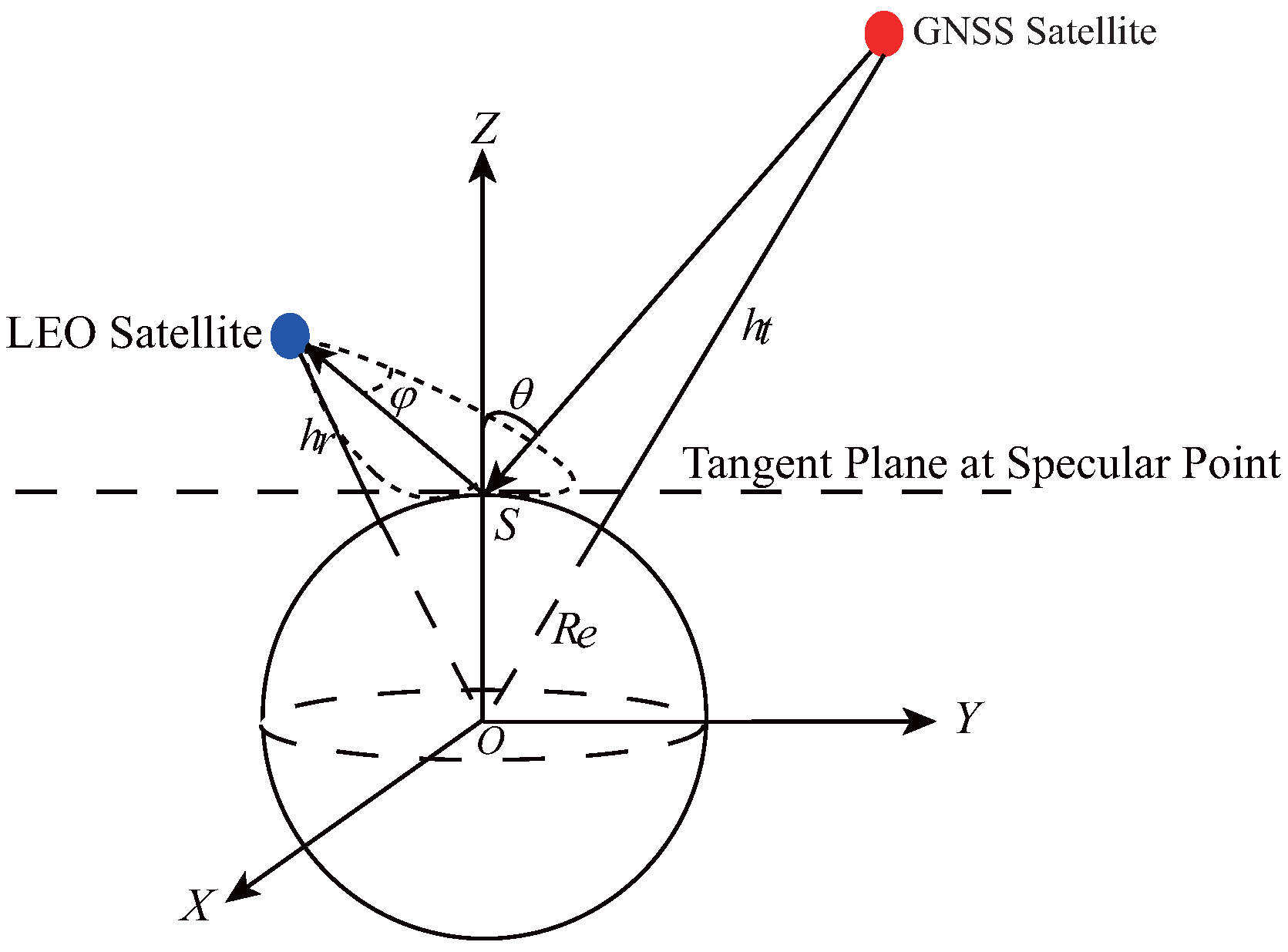
Figure 2.
Exponential distribution of (a) reflected GNSS signals for UK-TDS-1 satellite and (b) simulated data using scattering and noise models. The dotted lines are the best least squares fit using exponential function.
Figure 2.
Exponential distribution of (a) reflected GNSS signals for UK-TDS-1 satellite and (b) simulated data using scattering and noise models. The dotted lines are the best least squares fit using exponential function.

Figure 3.
Standard deviation vs. number of incoherent averaging for the UK-TDS-1 data. The dotted line shows the expected decrease as Equation (8).
Figure 3.
Standard deviation vs. number of incoherent averaging for the UK-TDS-1 data. The dotted line shows the expected decrease as Equation (8).

Figure 4.
Change of the delay difference between direct and reflected signals with being , (a) being , being ; (b) being , being .
Figure 4.
Change of the delay difference between direct and reflected signals with being , (a) being , being ; (b) being , being .

Figure 5.
Incoherently averaged delay waveform with being , (a) being , being ; (b) being , being .
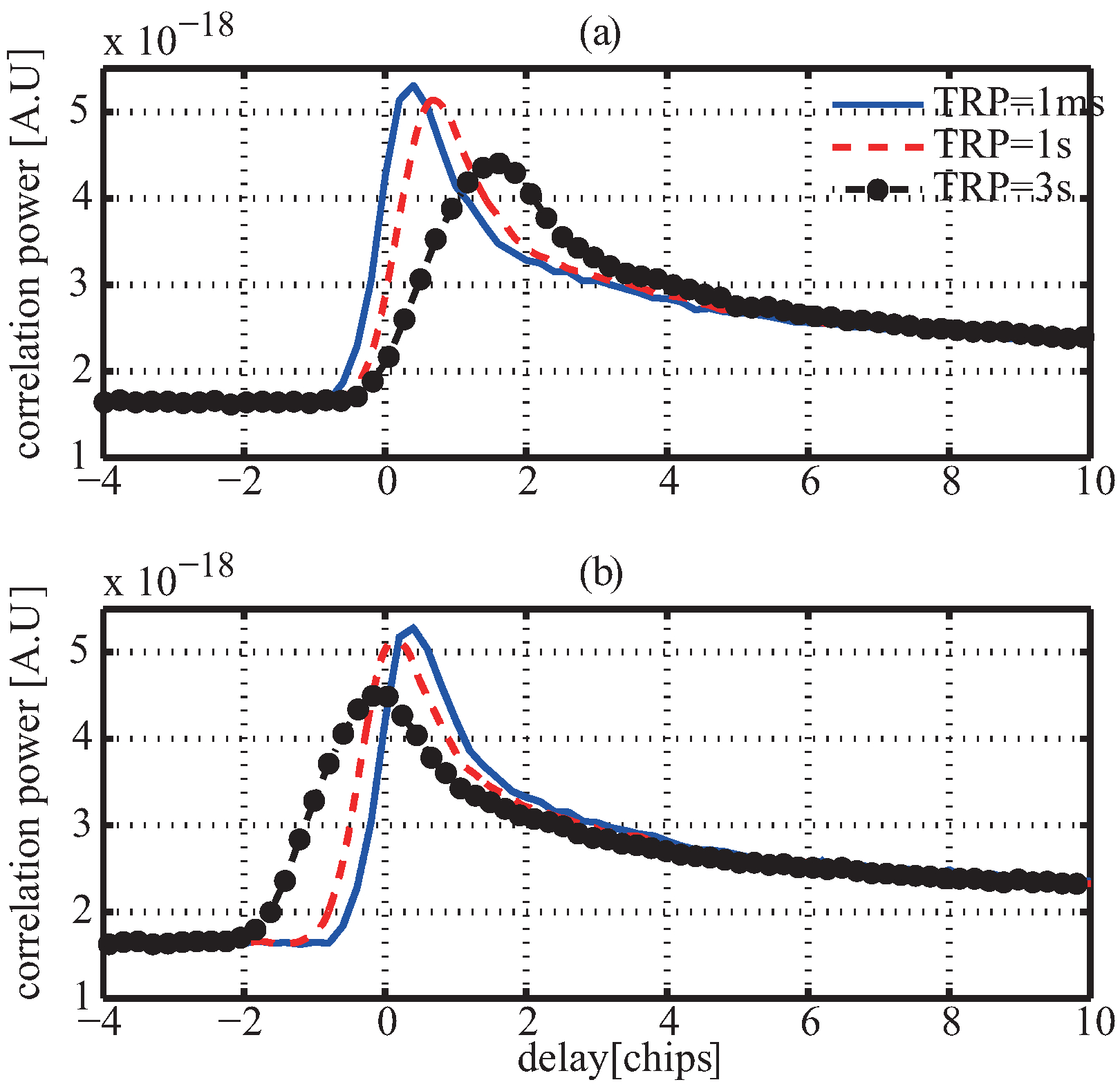
Figure 6.
Simulated and computed DDCR with being , (a) being , being ; (b) being , being .

Figure 7.
Sensitivity of (a) peak waveform; (b) leading edge slope; and (c) trailing edge slope on wind speed before and after retracking under the condition of the moving direction of LEO and GNSS satellite are both ; and the incidence angle is .
Figure 7.
Sensitivity of (a) peak waveform; (b) leading edge slope; and (c) trailing edge slope on wind speed before and after retracking under the condition of the moving direction of LEO and GNSS satellite are both ; and the incidence angle is .
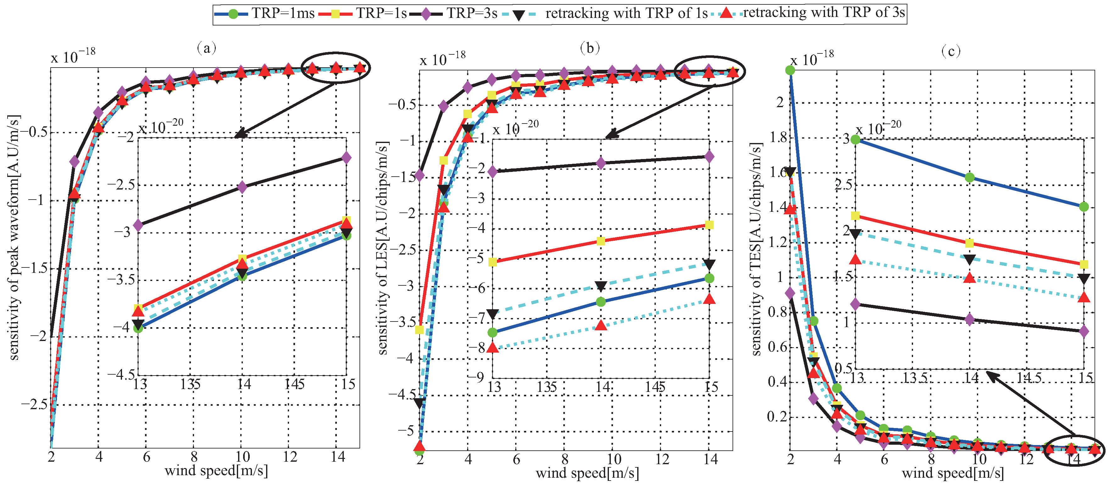
Figure 8.
Simulated delay waveform and fitted curve using analytic Model (20).

Figure 9.
On-ground retracking processing of distorted waveform.

Figure 10.
Delay waveform with the tracking refresh period of 1 ms, (a) 1 s; (b) 3 s; and corresponding waveform after retracking using Equation (21) for UK-DMC.
Figure 10.
Delay waveform with the tracking refresh period of 1 ms, (a) 1 s; (b) 3 s; and corresponding waveform after retracking using Equation (21) for UK-DMC.
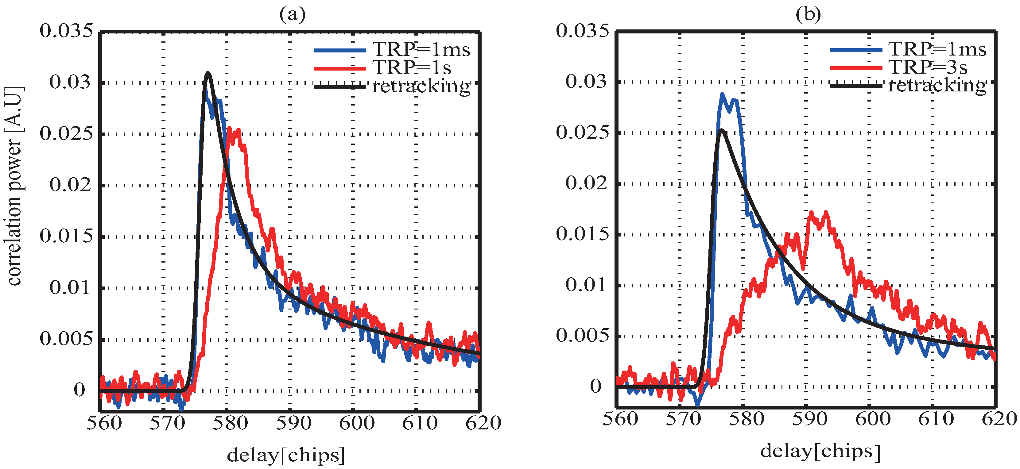
Figure 11.
Delay waveform with the tracking refresh period of 1 ms, (a) 1 s; (b) 3 s; and corresponding waveform after retracking using Equation (19) for UK-TDS-1.
Figure 11.
Delay waveform with the tracking refresh period of 1 ms, (a) 1 s; (b) 3 s; and corresponding waveform after retracking using Equation (19) for UK-TDS-1.

Figure 12.
Fitting error of PW, LES and TES between Z-V waveform and analytical Model (18).

Figure 13.
MSE between the retracked waveform and the one compensated on each correlation integration time period as the function of the DCR for (a) UK-DMC and (b) UK-TDS.
Figure 13.
MSE between the retracked waveform and the one compensated on each correlation integration time period as the function of the DCR for (a) UK-DMC and (b) UK-TDS.
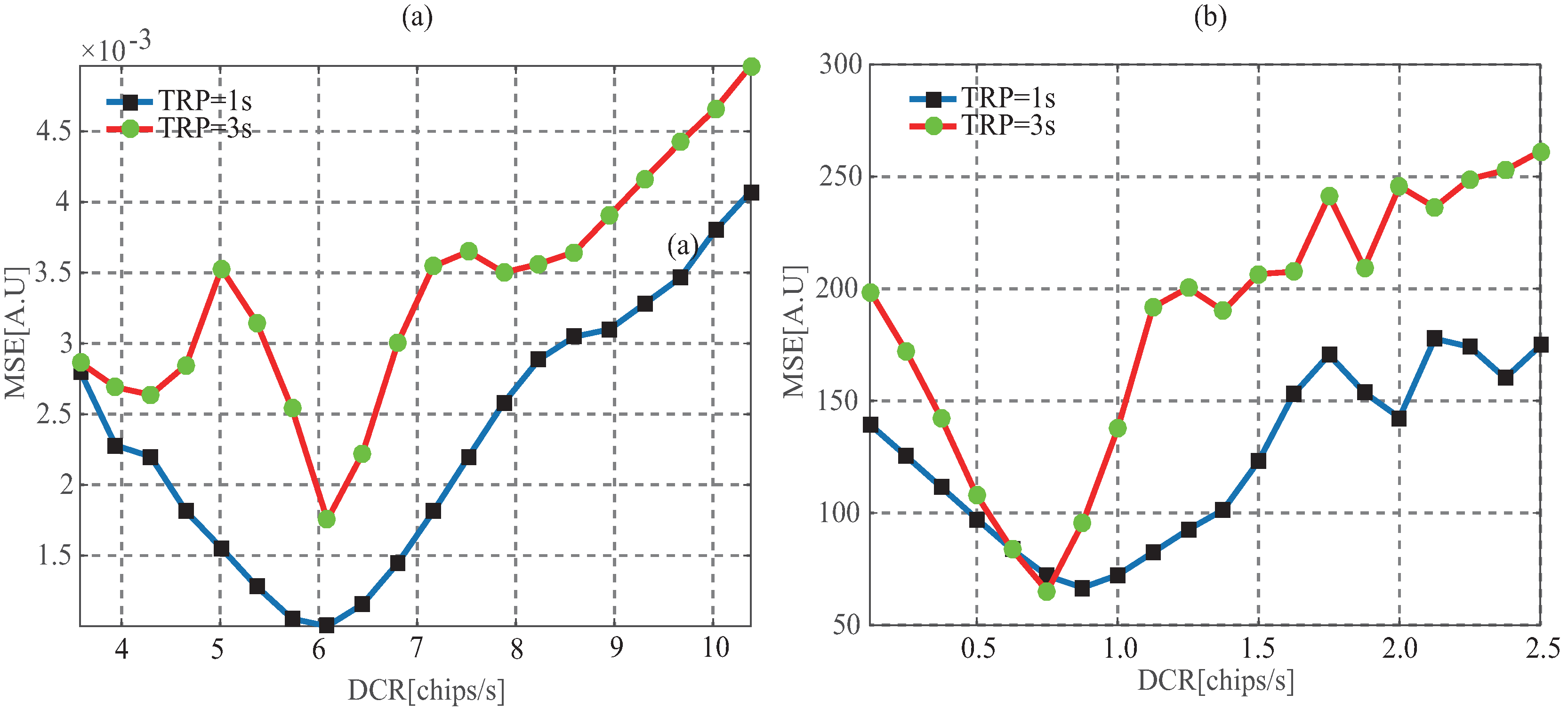
Figure 14.
Relationship between wind speed and peak waveform.

Figure 15.
Dependence of retracking performance for sea surface height on SNR.

Figure 16.
Dependence of retracking performance for wind speed on SNR.


Table 1.
The parameters of Simulation Scenario.
| Parameter | Units | Value |
|---|---|---|
| GNSS Satellite Height | km | 20,200 |
| LEO Satellite Height | km | 659 |
| GNSS Satellite speed | km | 3.07 |
| LEO Satellite speed | km | 7.60 |
| Earth Radius | km | 6371 |
| Maximum Gain | dB | 12 |
| 3 dB Beam Width | deg | 25 |
| incident angle | deg | [0:50] |
| Moving direction of GNSS Satellite | deg | [0:360] |
| Moving direction of LEO Satellite | deg | [0:360] |
| Coherent integration time | ms | 1 |
| Incoherent Integration time | s | 16 |
| Tracking Refresh Period | ms | [1, 1000, 3000] |
| Wind Speed W | m/s | [1:20] |
Table 2.
Comparison of MSE between retracked waveform and the one with the TRP of 1 ms using proposed and CSL and TSVD for UK-DMC and UK-TDS-1 data.
Table 2.
Comparison of MSE between retracked waveform and the one with the TRP of 1 ms using proposed and CSL and TSVD for UK-DMC and UK-TDS-1 data.
| Methods | 1 s | 3 s | |||
|---|---|---|---|---|---|
| UK-DMC | UK-TDS-1 | UK-DMC | UK-TDS-1 | ||
| proposed | 0.026 | 70.10 | 0.044 | 61.80 | |
| CLS | 0.041 | 85.82 | 0.078 | 89.94 | |
| 0.103 | 111.90 | 0.115 | 202.57 | ||
| TSVD | 0.044 | 88.75 | 0.130 | 95.43 | |
| 0.116 | 86.79 | 0.329 | 202.74 | ||
Table 3.
Standard Deviations of Estimated sea surface height for Retracked and Non-Retracked Waveform. re. and non-re. is the Shorthand of Retracking and Non-Retracking.
Table 3.
Standard Deviations of Estimated sea surface height for Retracked and Non-Retracked Waveform. re. and non-re. is the Shorthand of Retracking and Non-Retracking.
| Parameter | 1 ms [m] | 1 s [m] | 3 s [m] | ||
|---|---|---|---|---|---|
| re. | non-re. | re. | non-re. | ||
| std | 4.66 | 6.19 | 40.98 | 11.49 | 125.45 |
Table 4.
Root Mean Square Error of Retrieval Wind Speed Using Retracked and Non-Retracked Waveform.
| Observable | 1 ms [m/s] | 1 s [m/s] | 3 s [m/s] | ||
|---|---|---|---|---|---|
| re. | non-re. | re. | non-re. | ||
| PW | 2.24 | 2.25 | 2.55 | 2.43 | 3.37 |
| LES | 1.48 | 1.92 | 2.88 | 2.42 | 4.42 |
| TES | 1.59 | 1.84 | 2.33 | 2.51 | 4.95 |
| combined | 1.27 | 1.37 | 1.73 | 1.45 | 1.88 |
© 2017 by the authors. Licensee MDPI, Basel, Switzerland. This article is an open access article distributed under the terms and conditions of the Creative Commons Attribution (CC BY) license (http://creativecommons.org/licenses/by/4.0/).
Share and Cite
MDPI and ACS Style
Wang, F.; Yang, D.; Li, W.; Yang, W. On-Ground Retracking to Correct Distorted Waveform in Spaceborne Global Navigation Satellite System-Reflectometry. Remote Sens. 2017, 9, 643. https://doi.org/10.3390/rs9070643
AMA Style
Wang F, Yang D, Li W, Yang W. On-Ground Retracking to Correct Distorted Waveform in Spaceborne Global Navigation Satellite System-Reflectometry. Remote Sensing. 2017; 9(7):643. https://doi.org/10.3390/rs9070643
Chicago/Turabian StyleWang, Feng, Dongkai Yang, Weiqiang Li, and Wei Yang. 2017. "On-Ground Retracking to Correct Distorted Waveform in Spaceborne Global Navigation Satellite System-Reflectometry" Remote Sensing 9, no. 7: 643. https://doi.org/10.3390/rs9070643
Note that from the first issue of 2016, this journal uses article numbers instead of page numbers. See further details here.