
Good Practices for Object-Based Accuracy Assessment

Earth and Life Institute, Université catholique de Louvain, 1340 Louvain-la-Neuve, Belgium
*
Author to whom correspondence should be addressed.
†
These authors contributed equally to this work.
Remote Sens. 2017, 9(7), 646; https://doi.org/10.3390/rs9070646
Submission received: 3 January 2017
/
Revised: 26 May 2017
/
Accepted: 19 June 2017
/
Published: 22 June 2017
(This article belongs to the Special Issue Advances in Object-Based Image Analysis—Linking with Computer Vision and Machine Learning)
Abstract
:Thematic accuracy assessment of a map is a necessary condition for the comparison of research results and the appropriate use of geographic data analysis. Good practices of accuracy assessment already exist, but Geographic Object-Based Image Analysis (GEOBIA) is based on a partition of the spatial area of interest into polygons, which leads to specific issues. In this study, additional guidelines for the validation of object-based maps are provided. These guidelines include recommendations about sampling design, response design and analysis, as well as the evaluation of structural and positional quality. Different types of GEOBIA applications are considered with their specific issues. In particular, accuracy assessment could either focus on the count of spatial entities or on the area of the map that is correctly classified. Two practical examples are given at the end of the manuscript.

1. Introduction
Accuracy assessment is an acknowledged requirement in the process of creating and distributing thematic maps [1]. It is a necessary condition for the comparison of research results and the appropriate use of map products. However, despite the fact that the need to carry out (and document) accuracy assessment is recognized by the scientific community, further attention to rigorous assessment is still needed [2]. A general framework of good practices for accuracy assessment has been described in [3,4] in order to guide the validation effort. However, as mentioned in [5], Geographic Object-Based Image Analysis (GEOBIA) validation has its own characteristics. It is, therefore, necessary to adjust some of the good practices of the general framework for the specific quality assessment of GEOBIA results. These practices depend on the type of geospatial database that is going to be extracted from the image analysis.
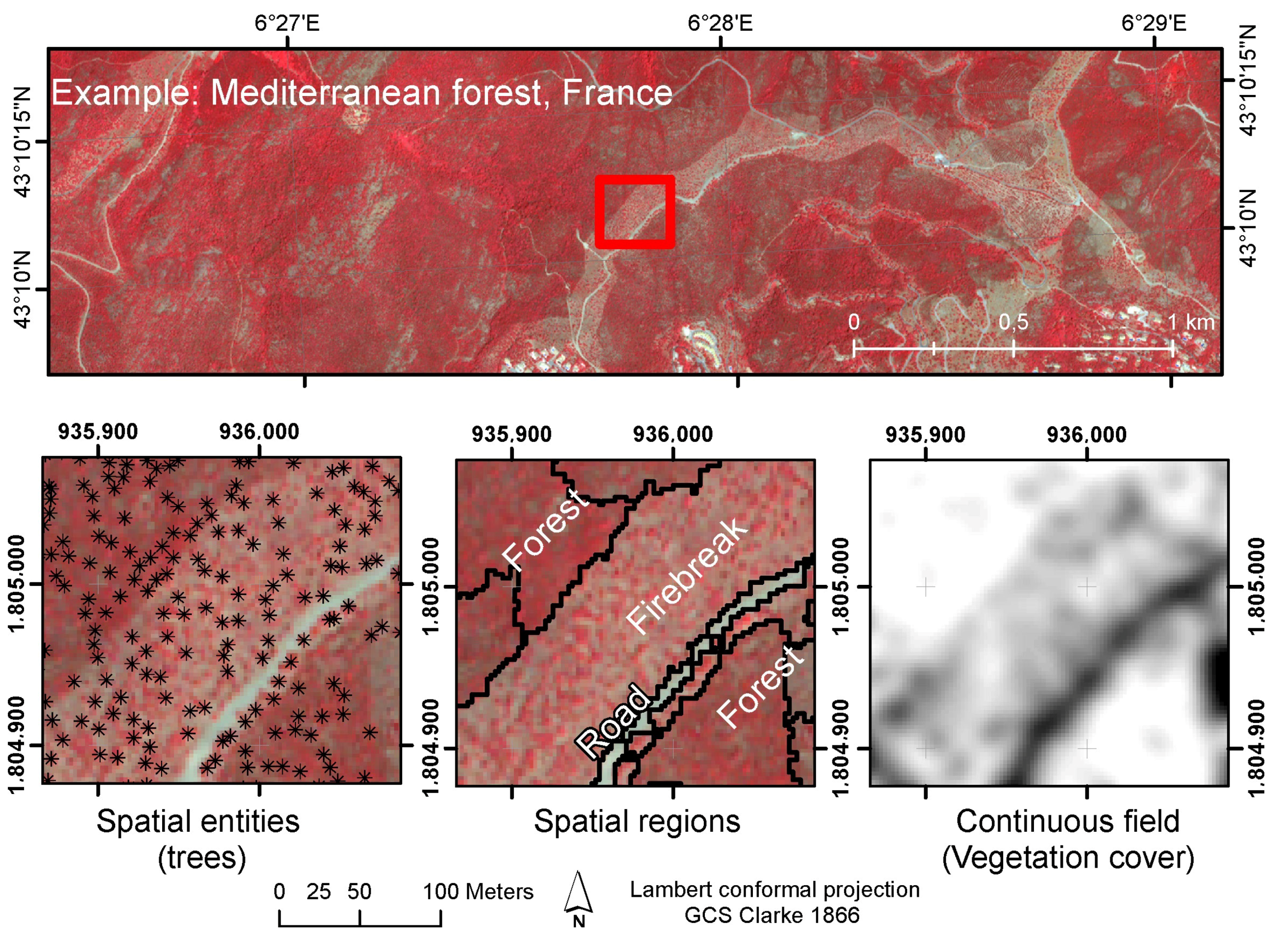
There are at least three important stages in the assessment process leading to the design of a geographic database: (i) observation, (ii) relating the observation to a conceptual model and (iii) representing the data in formal terms [6]. In the first stage, the surveyor must decide whether the observation is a clearly defined or definable entity, or if it is a continuum, i.e., a smoothly-varying surface. The first situation refers to an exact entity, called the discrete entity in Burrough [6] or the spatial object in Bian [7]. In this study, they will be named spatial entities. The second situation refers to a (continuous) field, and it is not well represented by GEOBIA [7]. However, viewing the world as either a continuum or as a set of discrete entities is always a matter of appreciation. At the level of the empirical, one-to-one scale geographic world, it is indeed not possible to decide if the world is made up of discrete, indivisible elementary entities, or if it is a continuum with different properties at different locations. On one side, houses, trees and humans are the non-subdivisible smallest units for most purposes of geographic-scale modeling and study; on the other side, extensive entities such as oceans, prairies, forest and geological formations may be subdivided within very wide limits and still maintain their identity [8]. A third category has therefore been added, which is called spatial region [7] or the object with an indeterminate boundary [6]. The term spatial region used in this paper represents a mass of individuals that can be conceptualized both as a continuous field and as discrete entity, which is often the case for land cover. This duality is also found for their coding in a database: they can be discretized as vector polygons with boundaries based on a general agreement (which are represented as adimensional lines, but which are fuzzy in reality), or they can be represented as an arbitrary grid specifying the proportion of each individual entity at each pixel (without boundaries) [7]. The three conceptual models (spatial entities, spatial regions and continuous field) are illustrated in Figure 1. The third model (continuous field) will not be discussed further in this paper.
GEOBIA is often considered as a new image classification paradigm in remote sensing [9]. It encompasses a large set of tools that incorporate the knowledge of a set of (usually) adjacent pixels to derive object-based information. GEOBIA is primarily applied to Very High Resolution (VHR) images, where spatial entities/regions are visually composed of many pixels and where it is possible to visually validate them [9]. Most of the time, these groups of pixels (called image-segments in Hay and Castilla [10]) are derived from automated image segmentation (e.g., [11]) or superpixel algorithms [12] before the classification stage. In addition to the frequently-used segmentation/classification workflow, some machine learning algorithms have been developed that recognize groups of pixels as a whole [13], and polygons are sometimes taken from ancillary data (e.g., [14,15]). In any case, GEOBIA relates to the conceptual model of geo-objects, defined as a bounded geographic region that can be identified for a period of time as the referent of a geographic term [16]. Geo-objects, which encompass spatial entities or spatial regions, are represented (and analyzed) as points, lines or (most of the time) polygons. GEOBIA then assigns a single set of attributes to each polygon as a whole, in contrast to pixel-based classification, where each individual pixel is classified. The polygons used in GEOBIA are thus intrinsically considered as homogeneous in terms of the label [10,17,18], even when those labels are fuzzy [19].
According to Bian [7], polygons are a good representation for spatial entities and a reasonable one for spatial regions, which might have indeterminate boundaries. Although many geographic-scale and anthropogenic entities have boundaries, the most precise boundaries existing in the geographic world are immaterial: these are administrative and property boundaries [8]. At the other extreme are the self-defining boundaries of social, cultural and biological territories. Extracting the boundaries is often part of the GEOBIA process, which then contributes to the discretization process. The quality of the boundaries should therefore most of the time be considered in addition to the thematic accuracy.
There is a wide range of applications of GEOBIA, and good validation practices depend on the selected application. In this study, we will focus on thematic (categorical) geographic database using the polygon representation of spatial entities or regions, as opposed to the pixel-based approach where the support of the analysis is the (sub)pixel captured by a sensor. With those thematic products, where a single category is assigned to each polygon (i.e., thematic maps), the accuracy of the labels assigned to the geo-objects is of primary concern. However, in addition to the thematic accuracy assessment, spatial quality should also be taken into account for GEOBIA [20]. The structural and positional quality of the polygons are therefore addressed, as suggested by [5]. The comparison of segmentation algorithms before the classification stage is, however, out of the scope of this paper, as this study will consider the quality of the final results, notwithstanding the specific numerical methods that were involved for their production. The proposed framework assesses thematic and geometric errors using distinct indices in order to identify the different sources of uncertainty for the derived product. Synthetic indices mixing the two types of errors (e.g., [21,22]) are therefore not discussed.
2. General Accuracy Assessment Framework
The general accuracy assessment framework defined in [3,4] is still applicable to most GEOBIA results. The standard practice consists of reporting the map accuracy as an error matrix when the map and reference classifications are based on categories [23]. Recommendations about the quality assessment are commonly divided in three components that have the same importance to draw rigorous conclusions and that should be reported to end users, namely the analysis, the response design and the sampling design.
Analysis includes the quality indices to be used to address the objectives of the mapping project, along with the method to estimate those indices [4]. Quality indices that are directly interpretable as probabilities of encountering certain types of misclassification errors or correct classifications should be selected in preference to quality indices not interpretable as such [24]. In order to derive unbiased estimation of these indices, the probability to select each sampling unit should be considered.
Response design is the protocol for determining the ground condition (reference) classification of a sampled spatial unit (pixel, block or polygon) [25]. The fundamental basis of an accuracy assessment is a location-specific comparison between the map classification and the “reference” classification [1]. The response design includes the choice of a type of sampling unit and the rules that allow the operator to decide if a sampling unit was correctly labeled (or not).
The sampling design is the way a representative subset of the geospatial database is selected to perform the accuracy assessment. In practice, it is indeed impossible to have precise (low uncertainty) and exact (unbiased) information that exhaustively covers the study area [4,25], except when using synthetic data. A subset of the geo-objects is, therefore, selected in order to estimate the accuracy of the map. The subset should be drawn with a probabilistic method, in order to be representative of the whole study area [23]. The sample can be stratified (i) to increase the proportion of samples in error-prone areas in order to reduce the variance of the estimator [26,27] and/or (ii) to balance the number of sampling units for each category in order to avoid large variances of estimation for low frequency classes [4].
As discussed above, GEOBIA can be oriented towards objectives, related with two different conceptual models: spatial regions or spatial entities. Furthermore, GEOBIA can have different goals. In an attempt to provide pragmatic guidelines, four types of GEOBIA applications are considered in this paper:
- Wall-to-wall mapping: This is the most common application, which results in thematic maps proposing a complete partition of the study area into classified polygons, such as for land cover or land use maps.
In the following sections, specific GEOBIA issues will be addressed with respect to these four types of applications, when relevant. Section 3 lays focus on the way to analyze the confusion matrix to estimate relevant quality indices. Section 4 is related to the response design and addresses the choice of the sampling unit (pixel or polygon). The methods to create a subset of polygonal sampling units are then described in Section 5. Finally, Section 6 addresses further issues related to the scale of the GEOBIA application, as well as specific geometric errors linked to the segmentation process.
3. Analysis of Quality Indices
For a pixel-based validation, the proportion of correctly classified pixels (count-based classification accuracy) is equal to the proportion of the area that is correctly classified (area-based map accuracy). In other words, if one knows how many pixels are misclassified, one also knows the area of the map that is misclassified. Indeed, standard validation procedures usually assume that pixels have all the same area (assuming pixels of equal area makes sense at small scale factor, but a rigorous pixel-based quality assessment over large areas should take into account that some coordinate systems do not preserve equal areas). Polygons, however, do not necessarily have the same areas, and their differences in size can be very large in some landscapes (e.g., a landscape including anthropogenic buildings and forests at the same time). In terms of the proportion of the area of the map that is incorrectly classified, an error for a large polygon has obviously more impact than an error for a smaller one. This variable area must be taken into account for an unbiased estimate of some accuracy indices.
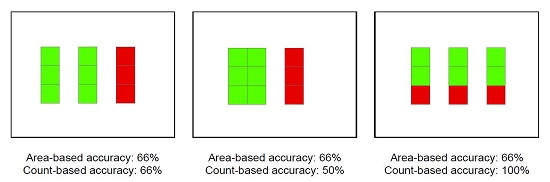
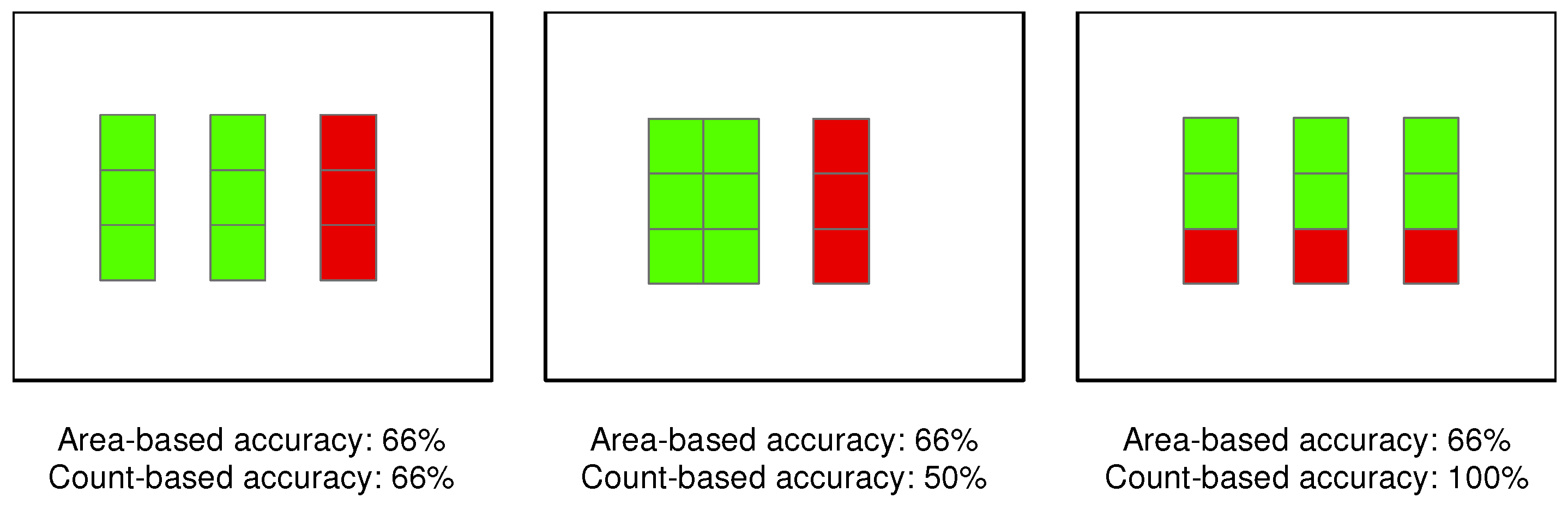
Figure 2 illustrates the differences between count-based and area-based accuracy on simplified examples, and it emphasizes the need of selecting indices that are meaningful for the purpose of the study. On one side, count-based accuracy (Section 3.1) should be used for the assessment of spatial entity detection, and on the other side, area-based accuracy (Section 3.2) should be used for spatial region mapping and for the classification of pixels. In the case of spatial entity delineation, the geometric precision is usually more important than the thematic accuracy. Nevertheless, the automated delineation could sometimes misclassify some of the spatial entities. Count-based indices can then be useful to estimate the probability of missing entities.
3.1. Accuracy of Spatial Entity Detection
In the case of entity detection, the validation process focuses on correct detection rates. In a binary classification, the response design identifies four possible cases: (i) the True Positives () are the entities that are correctly detected by the method; (ii) the False Positives () are the polygons that are incorrectly detected as entities; (iii) the False Negatives () are entities that are not detected by the method; and (iv) the True Negatives () are the correctly undetected polygons. Indices based on true and false detections are widely used in computer science and related thematic disciplines. However, GEOBIA detection does not solely rely on the classification of entities. Indeed, for polygons that have been classified as a spatial entity, over-segmentation (more than one image-segment for one spatial entity) and under-segmentation (more than one spatial entity encapsulated inside one image-segment) contribute to the false positives and the false negatives, respectively. As a consequence, the number of subparts minus one should, therefore, be counted as false positive, and the number of encapsulated geo-objects minus one should add to the false negative in these situations.
In the binary case, e.g., detection of dead trees in a dense population of trees, Powers [38] suggests three indices to summarize the information of the contingency table that is relevant for the comparison between methods, namely the informedness (Equation (1)), the markedness (Equation (2)) and the Matthews’ correlation coefficient (Equation (3)), with:
However, in most spatial entities’ detection context, is indeterminate because it would correspond to the background, which is not of the same nature as the spatial entities and is usually not countable (e.g., cows (spatial entities) in a pasture (spatial region)). In those cases, the count-based user accuracy (also called positive predicted value, Equation (4)) and the count-based producer accuracy (also called sensitivity, Equation (5)) provide a better summary of the truncated confusion matrix, where:
It is furthermore easy to show that the users’ and producers’ accuracies for the various classes are equal to the corresponding markedness and informedness for these classes when tends to infinity (i.e., if all pixels of the background were considered as ).
In addition, Count Accuracy () has been widely used in remote sensing applications, such as tree counting [39] or animal counting. It consists of dividing the number of detections ( and ) by the number of geo-objects in the reference, with:
While this index provides meaningful information at the plot level for documenting, e.g., the density of trees in a parcel or the total number of animals in a landscape, it does not provide location-specific information due to commission and omission errors that are canceled by the aggregation [40]. We therefore recommend to compute on a set of randomly selected regions of equal areas, in order to provide an estimate of its variance in addition to its mean value.
3.2. Accuracy of a Wall-To-Wall Map
For wall-to-wall maps, the area of the map that is correctly classified is the main concern. The primary map accuracy indices suggested by the comparative study of Liu et al. [41], namely overall accuracy, producers’ accuracies and users’ accuracies are recommended. Pixel-based accuracy estimators and their variance can be found in the general good practices from Olofsson et al. [4]. For GEOBIA results, the same indices should be used. However, with polygon sampling units, the estimators of the primary accuracy indices should take the variable size of polygons into account in order to avoid bias and to reduce the variance of the predictors.
In the context of polygon-based estimation of the thematic accuracy, correctly classifying large polygons will contribute more to the map quality than correctly classifying smaller ones. Unbiased predictors of the primary accuracy indices have, therefore, been suggested in Radoux and Bogaert [42]. Under the hypothesis of binary agreement rules and representative samples, these indices use the knowledge about the area of the polygons to predict overall accuracy (Equation (7)), user accuracies (Equation (8)) and producer accuracies (Equation (9)), with:
where N is the total number of polygons in the map, n is the number of sampled polygons and is the area of the i-th polygon. , are binary indicators of the actual and predicted labels j of polygon i. is therefore equal to one, if the i-th polygon was correctly classified, and zero, otherwise. is an estimate of the probability to belong to class j, and is an estimate of the classification accuracy ( is the set of all possible classes in the map). The main difference with the classification accuracy estimated with the standard point-based estimators is the inclusion of the size of the polygons in the first term of the numerators of each equation. Furthermore, the area of the non-sampled polygons is also taken into account, so that all information at hand about the polygons is used. Finally, it is worth noting that the second terms of the numerators of Equations (7)–(9) have more influence when the number of polygons is large: the above predictors simplify to the standard estimators when N becomes infinite if the count-based accuracy is not influenced by the size of the polygons.
Relationships between size and classification accuracy have been highlighted in previous studies [42,43] and could impact the predictors. In theory, these relationships can be plugged into Equations (7)–(9) by replacing with a function of the size (Radoux and Bogaert [42]). In practice, it is not trivial to identify this function and to estimate its parameters. A pragmatic solution consists of (i) splitting the sample based on quantiles for the areas of the polygons, then (ii) estimating for each size category q and, finally, (iii) multiplying by the sum of the polygons’ areas in that size category q. Another solution consists of estimating the area-based accuracy from the sampled polygons only, with:
where n is the number of polygons in the sample. This formula (that can be adapted for both users’ and producers’ accuracy estimates) has a larger variance than Equation (7), but it is unbiased. It is therefore of appropriate use, when the size of the sample is small and is difficult to estimate.
So far, the best approximation of the prediction variance of the overall accuracy estimator given by Equation (7) is:
which can be used to derive the confidence interval around the predicted overall accuracy index (to the best of our knowledge, there are no simple formulas for the prediction variance of the polygon-based users’ and producers’ accuracies). Equations (7)–(9) will be particularly efficient when the number of polygons in the map is small, and they are at least as efficient as a point-based sampling when the number of polygons is very large [44].
4. Response Design
The response design encompasses all steps of the protocol that lead to a decision regarding the agreement of the reference and map classifications [4]. Response design with GEOBIA is an underestimated issue. Indeed, because classification systems involved in GEOBIA are often complex, not only accuracy issues (e.g., mistaken photo-interpretation), but also precision issues (e.g., difficulty to estimate the proportion of each class of the legend) could affect the quality of the reference dataset.
The sampling unit must be defined prior to specifying the sampling design, and it is not necessarily set by the map representation [25]. In the case of GEOBIA, the use of polygons sampling units is usually recommended [27,45] because the legend is defined at the scale of the polygons and not at the scale of the pixels. However, there is no universal agreement on a best sampling unit [1]. In order to select a type of sampling unit, the conceptual model and the sampling effort must indeed be taken into account.
For spatial entities, polygon sampling units prevail because distinct individual entities are extracted. Individual pixels indeed need to be aggregated at different levels to compose a geo-object. For instance, a high resolution pixel identified as a window could be the windshield of a vehicle or the skylight of a building roof top. The photo-interpretation of very high resolution images, therefore, intrinsically takes context into account to identify spatial entities. The response design should, however, include rules for handling imperfect matches between the reference and the image-segment. Topological relationship, such as intersection or containment, based on the outlines or the centroids, define unambiguous binary agreement rules with a tolerance for delineation errors. Alternatively, an entity may be considered correctly labeled if the majority of its area, as determined from a reference classification, corresponds to the map label [1].
For spatial regions, various classes (e.g., urban area, open forest, mixed forest, orchard) are also defined at the polygon level and would not exist at the scale of a high resolution pixel [46]. Those classes typically (i) represent complex concepts where the context plays a major role for the interpretation or (ii) generalize the landscape. The generalization of the landscape offered by GEOBIA may better represent how land cover interpreters and analysts actually perceive it [36]. The selected legend is then strongly related to the scale at which a spatial region is observed and linked with minimum mapping units, which are not necessarily identical for all classes (e.g., [47]). However, when using polygons as sampling units, one should make sure that the object-based generalization is suitable to represent the variable of interest. Otherwise, pixel sampling units are more relevant.
When polygon sampling units are selected, the rules that define the agreement are usually simpler when the reference data are based on the same polygons as those on the map. Nevertheless, object-based quality assessment could need information about the segmentation quality in addition to the thematic accuracy assessment. As discussed in Section 6.1 and Section 6.2, manually digitized or already existing polygons of reference may then be needed. The use of manually digitized polygons for the assessment of the thematic accuracy is however complex because the aggregation rules are then applied on different supports.
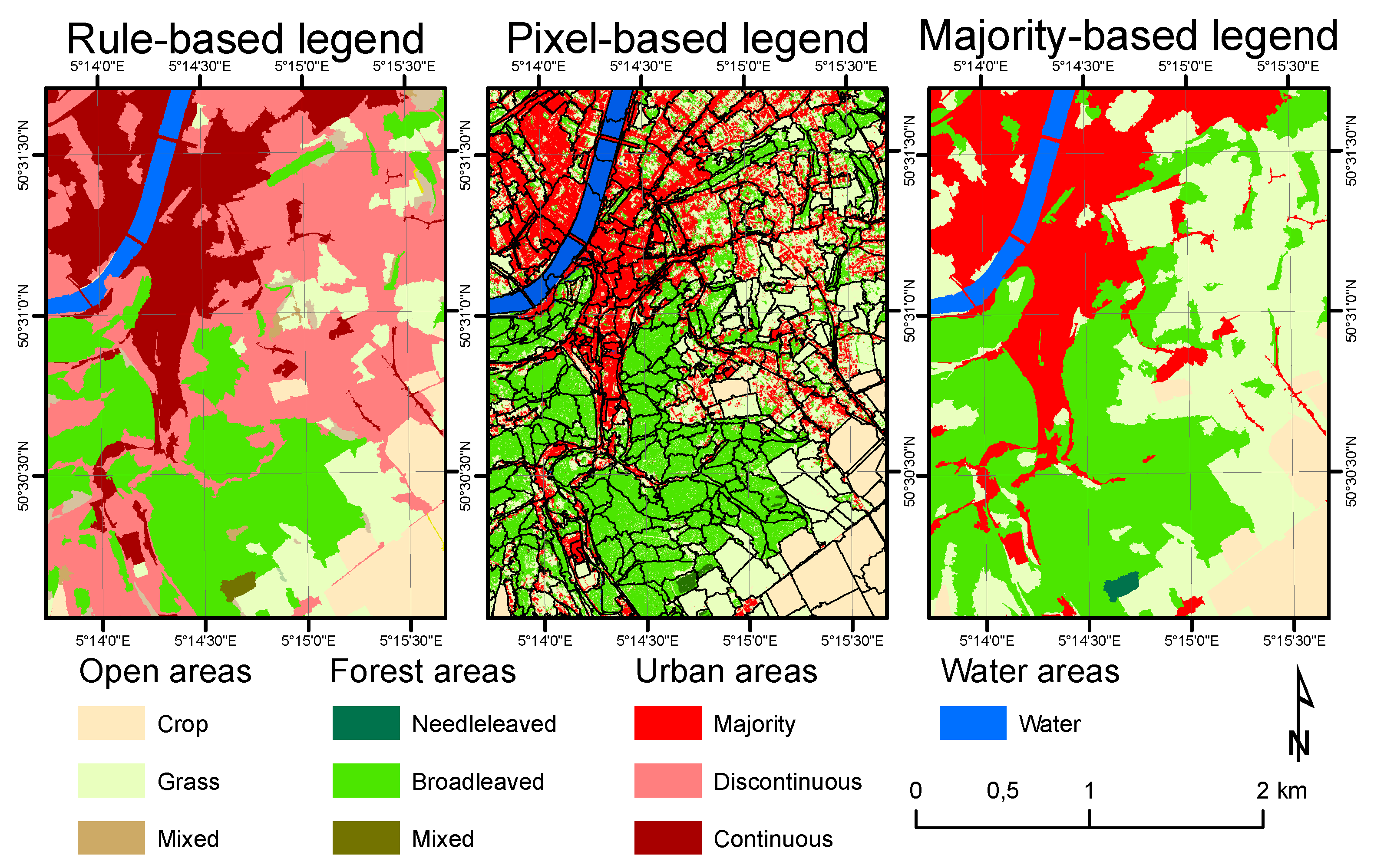
Issues related to the heterogeneity of polygon sampling units are similar to the so-called mixed pixels problem. It is therefore of paramount importance to clearly define the labeling rules in order to avoid ambiguous validation results. There is however no universal set of decision rules that fits to all mapping purposes. As a consequence, the same landscape can be described with different legends (e.g., Figure 3), which cannot be compared without a fitness to purpose analysis. For the thematic accuracy assessment, the response design links the observed reality to the type of legend of that has been selected for the map. Those legends can be categorized into majority-based, rule-based (such as the Land Cover Classification System (LCCS) [48]) or object-oriented :
- Majority rules assign a label based on the dominant label inside each polygon. The legend includes the minimum number of classes necessary to represent each of type of geo-object that are identified with a smaller scale factor. The labeled polygons are usually interpreted as “pure” geo-objects. It is, therefore, most suited when GEOBIA aims at identifying spatial entities, but is frequently used with spatial regions, as well. In this case, the polygons are used to generalize the landscape (e.g., mapping the forest and not the trees) or to avoid classification artifacts. When there are more than two classes, it is worth noting that the majority class could have a proportion that is less than . Majority rules could therefore be source of confusions.
- Rules-based legends (e.g., FAO LCCS rules) are built upon a set of thresholds on the proportion of each land cover within the spatial unit. When correctly applied, those rules generate a comprehensive partition of all of the possible combinations of its constitutive spatial entities. They are well suited to the characterization of complex land cover classes using spatial regions. Each LCCS class is characterized with a unique code that guarantees a good interoperability.
- The goal of object-oriented legends is to build human-friendly representations of geo-objects based on the knowledge that people cognitively have about the geospatial domain [49]. The conceptual schema describing information are linked with formal representation of semantics (i.e., ontologies) [50] in an attempt to capture and organize common knowledge about the problem’s domain. The concepts are often well understood (e.g., an urban area), but difficult to quantitatively define. Land use and ecosystem maps belong to this category. Each concept has a set of properties and relations between spatial entities, which involve geometric and topological relationships.
When GEOBIA is used as a means to improve classification results at the pixel level, treating a polygon as homogeneous could lead to a biased estimate of the number of pixels in a class. In order to properly assess the impact of GEOBIA on pixel classification, it is therefore suggested to use pixel-based sampling units. Indeed, the alternative method combining object-based thematic accuracy assessment and a measure of the polygons heterogeneity is likely to be less cost effective to achieve the same results.
The variance of the overall accuracy estimation with polygon sampling units is smaller or equal to the variance of a pixel-based validation under the same type of sampling scheme and with the same number of sampling units [51], but there are two disadvantages of using polygon sampling units. Firstly, the response design with polygons is often more complex than with pixels, especially when geometric quality needs to be assessed. Polygon-based validation therefore does not necessarily reduce the total sampling effort. Secondly, polygon sampling units are bounded to a given partition of the landscape. They are therefore difficult to reuse for change detection [25] if the same segmentation is not used for all dates.
5. Sampling Design
5.1. Sampling Scheme for Polygons
In practice, it is usually not possible to apply a response design to the entire map. A sampling design is then used to select a subset of the polygons that aims to be representative of the whole dataset. In relationship with the analysis section, the sampling design should be based on the polygons list in order to achieve equal probability sampling for each polygon. A pragmatic solution consists in randomly shuffling the list of polygons, then selecting the n first ones. This method yields an equal probability sample without replacement. In contrast, the selection of polygon sampling units based on randomly selected pixels on the map will select polygons with a probability proportional to their area [1]. This method should, therefore, be used with care, because existing estimators of the quality indices assume an equal probability sampling. For the same reason, systematic sampling cannot rely on the selection of regularly spaced polygons. Alternatively, a regular coverage of the study area with nearly equal probability sampling can be achieved by randomly selecting one polygon inside each cell of a regular grid several times larger than the average size of the polygons.
Because the classification accuracy also depends on the size of the polygons, Stehman and Wickham [1], Hernando Gallego et al. [5] suggested to stratify the sampling, based on categories for the polygon areas. This kind of stratification could replace a class-based stratification because polygon area is also correlated with class probability [42]. Accounting both, for these areas and class probabilities in the stratification, could thus be unnecessary and would produce too many bins, which would result in less reliable estimations of the users’ and producers’ accuracies. In any case, the area covered by each strata should be used to adjust the estimates of indices accuracy, as a generalization of the equation of Card [52] for pixel-based stratification:
where is the proportion of the area of the stratum k that is correctly classified and is the proportion of the area of the map covered by the stratum.
5.2. Sampling Scheme for Entity Counting
Most of the time, detected geo-objects only cover a portion of the area of interest. A sample of spatial entities detected by the image analysis is, therefore, unable to measure the omission errors. On the other hand, spatial entities may cover only a small part of the area. Building a reference dataset based on random point-based sampling is not practical, because the sampling probability of the spatial entities would be too low. An external wall-to-wall dataset with the location of the spatial entities is therefore needed. When the exhaustive validation of the study area is impractical, region-based sampling can be used to provide a subset of territory from where to extract reference data. Whiteside et al. [20] used buffers around random point samples; however, systematic sampling based on regular grids [53] (or beehives) is a sound alternative.
6. Geometric Precision
When the boundaries are extracted during the GEOBIA process, information about their quality could be needed. The boundary extraction depends on the scale of the analysis (scale is the great boundary maker according to Couclelis [8]) and on the resolution of the input data. We must therefore distinguish two uncertainty types: we may be uncertain (i) with respect to the precise location of a crisp boundary due to measurement errors or (ii) with respect to indefinite correspondence between concepts (e.g., ecotone) and the represented world [8]. Furthermore, there is a duality between the definition of a boundary and the definition of its interior. The geometric quality of the delineation can, therefore, focus more either on the interior of the geo-object (structural quality) or on its boundaries (positional quality), depending on the application.
6.1. Structural Quality
Structural quality is related to the ability of the polygon to enclose a specific patch [5]. Structural quality depends on the segmentation quality and can, in turn, affect the thematic quality. The two facets of structural quality are over-segmentation and under-segmentation. On the one hand, over-segmentation consists in subdividing an geo-object into two or more smaller polygons. It is usually due to a larger-than-needed scale of analysis. On the other hand, under-segmentation consists of including sizable parts in the interior of the polygon that had rather been placed in a different polygon. The impact of over- and under-segmentation on the quality of the product depends on the purpose of the analysis.
Structural quality is particularly important in the case of entities detection because it directly impacts the geo-objects count. Under-segmentation can induce under-detection, while over-segmentation tends to contribute to an overestimation of the number of geo-objects. Over- and under-segmentation are quantified based on the comparison between the polygons and reference polygons (often manually delineated on the image). Under-segmentation is measured by the number of mapped polygons having their centroids inside the reference polygons and the opposite can be done for over-segmentation [32]. However, in practice, it may not be necessary to derive specific indices related to over- and under-segmentation in the case of spatial entities. Indeed, as mentioned in Section 3, over-segmentation errors are already contributing to the count of true positives (hit) and under-segmentation errors will increase the number of false negatives (miss).
For area-based mapping, it is commonly accepted that a poor quality of the segmentation leads directly to a low quality of the classification [54]. However, over-segmentation does not have a direct impact on the final quality because correctly classified polygons can be merged after classification if necessary [55]. For instance, Grenier et al. [56] used merged polygons from different levels for validation. Over-segmentation could, however, affect the thematic accuracy, as previous studies highlighted that the classification accuracy depends on the size of polygons [42,43], but its impact is not always negative. As this impact can be measured by the thematic accuracy indices, investigating over-segmentation is not necessary for spatial region mapping.
On the other hand, under-segmentation can adversely impact the quality of the map because subparts are missing. The definition of the classes then plays a major role in the accuracy assessment and could lead to major misunderstandings. GEOBIA is indeed often linked with a data model representing a continuous reality with discrete boundaries [57]. As discussed in the introduction, spatial heterogeneity is a component of many spatial regions and entities. For instance, a car loses its functionality if its wheels are removed, and a savanna would not host the same animal species with a continuous tree cover. Heterogeneity is, therefore, not necessarily an undesired characteristic of geo-objects, but it can be optimized at a given scale.
The response design (Section 4) should take heterogeneity into account and specify when individual parts compose the geo-objects (e.g., windows on a roof top of a building, sparsely distributed trees in an open forest) and when they are erroneously included (e.g., island in a lake). In the case of an inclusion, a minimum mapping unit is needed to determine if the polygon is correctly delineated. This minimum mapping unit is linked to the scale of the map, but can also differ for each class of a geographic database because geo-objects occur at different scales [47].
From a quality assessment perspective, under-segmentation should thus be considered as a precision issue and not an accuracy issue. A well defined legend indeed includes decision rules for all possible associations of individual parts, so that each predicted label can be matched with a corresponding reference label. However, the variance of the proportions of elementary units inside each polygon is larger when there is a large probability to have inclusions. A GEOBIA product with large under-segmentation issues could, therefore, be accurately labeled, but might provide imprecise estimates of the area covered by elementary units.
In practice, assessing the structural consistency of the polygons would be very time consuming because it is similar to the area-based accuracy assessment of a map, but applied to each sampling unit. A wall-to-wall approach, similar to the area-based segmentation goodness indices [58], can thus be used for each polygon. In practice, this level of quality assessment is only necessary for the delineation of spatial entities, and it is sometimes useful for large spatial regions.
6.2. Positional Quality
Due to the scale of the errors, positional quality of polygons has less impact on the thematic quality assessment than pixel sampling units [1]. However, positional errors do affect the map quality. Those errors could be due to (i) geometric errors in the source data or (ii) delineation errors resulting from the segmentation process. Information about the spatial precision of the map should, therefore, be provided in order to document the scale at which it can be used, and to detect potential bias due to the difference between the actual boundaries and those observed by remote sensing. The uncertainty on the position of these boundaries may come from different sources: (i) the spatial resolution of the sensor; (ii) orthorectification errors (e.g., residual parallax along large height gradients); (iii) segmentation errors; (iv) fuzziness due to gradual transitions between adjacent regions (e.g., ecotone) and (v) fuzziness due to variability over time (e.g., sea shore).
The boundaries of spatial entities are usually sharp and easy to describe with a set of widely accepted rules. However, the actual position of the boundary between two spatial regions is often fuzzy (e.g., ecotone between two biotopes). Previous studies further showed that some geo-objects were more complex to accurately digitize than others, and that there was a high degree of variability among image interpreters when hand-digitizing the same geo-objects [59]. The geometric precision of GEOBIA should, therefore, focus on true land cover transitions when available [5], while median boundaries are recommended when the photo-interpreters disagree [60].
In order to document the uncertainty of the position of the boundaries, the distance between the reference boundaries and the corresponding boundaries in the geographic database has to be measured. The Root Mean Square Error () or (the radial error, which of all errors in a circular distribution will not exceed) [61], are standard indices to report positional errors and are directly related to the cartographic scale. There is no standard method to estimate these errors, but two types of approaches have been proposed:
- Surface-based methods consider the geo-object as an entity to be compared with a polygon of reference. Areas of the controlled polygons in and out of the reference polygon are then measured for different buffer sizes [17] so that the proportion of correctly delineated geo-objects is reported for a set of distances. This method can thus be used to empirically determine the buffer distance that embeds a given proportion of the errors [62].
- Edge-based methods measure some statistics about the distance between the reference edge and the delineated edge. The RMSE can be derived from point samples along the reference boundaries compared with their perpendicular projection on the polygon boundaries [63]. The mean absolute error is estimated by dividing the area of mismatch by the length of the boundary [5,64]. The proportion of the boundaries within a given tolerance has also been suggested [21]. These methods are more difficult to implement, but can be useful to describe the errors for different types of edges. The fuzziness and the measurement errors indeed depend on the type of edges [6,63].
Alternative methods looking at the boundaries include a comparison of the distance between vertices [58] or the overlap of buffers around the perimeters of the two geo-objects [65]. They are, however, more difficult to relate to scale: the former could be affected by the density of vertices and the latter is not designed to reach because the same buffer is applied to each boundary.
7. Overview of the Recommended Practices
Details about the quality assessment of GEOBIA products with a crisp classification are provided in the previous sections. From a more pragmatic viewpoint, it is not necessary to estimate all indices in all cases. Table 1 summarizes the recommended practices with respect to the objectives of the GEOBIA described in Section 2.
One needs to first identify if GEOBIA is used to enhance per-pixel classification or if the conceptual model of the geographic database is better represented with polygons. In the first case, pixel sampling unit is recommended, because: (i) it simplifies the response design and (ii) it does not require specific boundary or structural quality control. Standard methods for the accuracy assessment of pixel-based classification (see [4]) are thus fully applicable in those cases.
When the legend is defined at the scale of the polygons, the thematic accuracy assessment should be based on the polygon sampling units. An appropriate response design should then take the conceptual model into account in order to define the binary agreement between the polygons and the “real world” (see Section 4). Within object-based conceptual models, GEOBIA products are usually either a wall-to-wall map of the landscape into (mainly) spatial regions, or a spatially discontinuous set of one (sometimes several) types of spatial entities. These two types of GEOBIA products should be validated with the set of indices that reflect their purpose.
In case of wall-to-wall mapping, (i) area-based accuracy assessment indices are recommended (Section 3) and (ii) additional information about the precision of the boundaries and the generalization of the content could be needed (Section 6). The response design should be based on the content of each polygon. Due to the variable size of those polygons, the area of each sampling unit has to be taken into account in order to provide an unbiased estimate of the accuracy indices.
Finally, studies dedicated to a set of spatial entities usually aim at either updating large scale vector maps (entity delineation) or inventorying a specific type of entity (entity counting). For the former, thematic accuracy is not a primary concern and the validation should focus on the geometric quality of the polygons (Section 6). For the latter, count-based quality assessment (Section 3.1) should be applied with a response design that addresses possible segmentation errors. However, the quality of the delineation is usually not an issue as long as the spatial entities are correctly detected. In case of poor delineation, the response design should clearly state the matching rules that define when a spatial entity has been detected.
8. Examples
8.1. Illustration of Tree Crown Detection
This example is a synthetic case study of a typical GEOBIA analysis where the purpose is to count a specific type of spatial entities. For instance, these could be houses, trees, tents, vehicles or animals. It is worth noting that, especially for vehicles and animals, the reference must come from the same image as the one that is used from the image analysis, therefore assuming that photo-interpretation will be closer to reality. Looking at images of the same sensor at different dates could further help to consolidate the photo-interpretation because it is unlikely that moving spatial entities remain exactly at the same place on two different dates.
In this case study, the photo-interpreters are asked to locate one point at the centroid of each spatial entity that they identify on the map. The response design considers here, as a match, a centroid that is closer than 2 m from the centroid of the corresponding reference entity. However, given that our simulated results include 11,000 points (see Figure 4), validating all of them would be cumbersome and a subset region has to be selected.
At this stage, only detected entities are available, and they are homogeneously distributed in the study area. A systematic region-based sampling without stratification is, therefore, selected. In other circumstances, the density of detected entities could be used to stratify the sampling.
A priori, the number of points needed to assess the quality of the GEOBIA results could be computed based on Equation (14), as in Olofsson et al. [4], with:
E.g., with an expected accuracy of , one needs approximately points to estimate the TP rate with a confidence interval d of at a 95% confidence level (for which ). With a grid of 100 cells, there will be 110 detected entities per cell on the average. Eight of those cells are, therefore, randomly selected to obtain a sufficient sample size, and reference data is then collected inside each cell (see Figure 4).
As the spatial entities are sparsely distributed, true negatives are undefined. Equations (4) and (5) are, therefore, used to estimate the user’s and producer’s accuracies based on the number of true positives (), false negatives () and false positives (), with:
When the sample is based on regions, the total number of sampling units is a priori unknown. Now that the total number of points is known for each sampled region and the accuracy indices have been estimated, the 95% confidence interval can be updated by replacing the guessed values with the observed values. Equation (17) gives the result for , which is approximately the same as for .
Finally, the count accuracy can be computed from Equation (6) for each cell, then the bias and the confidence interval on this quantity can be measured. In this example, omissions and commissions errors largely compensate each other, but there is a variability between cells. The here is equal to at confidence level. The confidence interval is based on the variance of the s computed for each sampled cell.
8.2. Wall-to-Wall Land Cover Map
The wall-to-wall land cover map presented here is a real case study and was produced in the framework of the Lifewatch European Research Infrastructure Consortium. The version assessed here is the first public release (Version 2.7), which was based on 25-cm-resolution aerial images of 2015, and LIDAR data from 2012/2013. It covers 16,844 km of the Walloon region (Belgium) with 1,000,000+ polygons.
A stratified random sampling is used for the validation, based on three super-classes: open areas (crops, pasture and vegetation mixtures with small tree cover), forest areas (broadleaved, needle-leaved, mixed forests, and vegetation mixtures dominated by trees) and others (sparse urban, dense urban, bare soils, water and wetlands). The classes are grouped in three strata in order to minimize confusions within them and to include all classes. The characteristics of each stratum is summarized in Table 2.
A lower accuracy was expected for the open areas stratum due to the low separability between some crops and pastures. More points were therefore selected in this category according to Equation (14), with values of , 0.9 and 0.9 for the overall accuracies of the Open areas, Forest areas and Other areas, respectively. Considering the large (>10) number of polygons in the map, Equation (14) can be used as a conservative approximation to compute the number of required sampling units. The number of validation samples was then empirically optimized for a precise estimation of the overall accuracy, aiming at a confidence interval of at a confidence level, with:
For each stratum, randomly selected polygons are validated by photo-interpretation based on orthophotos and ancillary data from authentic sources. The response design used threshold-based decision rules that are provided in the Appendix A. Table 3 summarizes the outputs in terms of number and area of polygons that are correctly classified within each group. In order to take into account the relationship between area and classification accuracy, the count-based accuracy was estimated with quantiles of polygons area. Three quantiles were used with the Open areas stratum and only two were used for the other strata, as a compromise between the number of bins and the precision of the estimates inside each bin. For the Open areas stratum, the count-based accuracy of the smallest polygons was significantly smaller than for the medium and largest polygons, with values respectively equal to , and . There is a significant size effect too for the Others stratum ( and respectively for small and large polygons), but there is no significant size effect for the Forest areas stratum ( and respectively for small and large polygons). As an example, the overall accuracy for the Other areas stratum is computed as:
by plugging the observed values in Equation (7). The area in the sample is 112 hectares of correctly classified polygons and the total area of the polygons from the Others stratum is hectares (see Table 2). The count-based accuracies estimated from the small and large polygons are multiplied by the total area of the small and large polygons in the set of non sampled polygons.
The overall accuracy of the whole map is computed as the weighted sum of the overall accuracy of each stratum (Table 3) based on their relative proportion (Table 2). The total overall accuracy value is . As the measured overall accuracies per stratum were different from the first guess used for the sampling design, the confidence interval needed to be updated. By reusing Equation (18) with the observed values, it was updated to .
Both count-based (Table 4) and area-based (Table 5) confusion matrices are presented in this example to highlight the differences between them. On average, there is an absolute difference of between the various users’ accuracies and between the various producers’ accuracies. The largest difference () is observed for the producers’ accuracy for water (W), because the omission errors occurred for very small polygons.
The structural quality of the polygons was quantified using the proportion of the dominant class. The average proportion within the sampled polygons was . As mentioned in Section 4, polygon heterogeneity is sometimes necessary to describe complex landscapes. However, it is often difficult to objectively decide when the structural quality could be improved. In this study, a larger average proportion was observed for correctly classified than for incorrectly classified polygons ( and , respectively). This tendency to better classify the homogeneous classes was also captured by the confusion matrix, where most of the errors occurred at the transition between two classes. This suggests that the thematic accuracy of the map could be improved if the under-segmentation was reduced or if the legend could be optimized for the specifically heterogeneous regions. On the other hand, the homogeneity is a very class-specific feature that is related to the landscape. Crop is the most homogeneous land cover in the study area (), closely followed by bare soil and water (>95%). Grassland, which might encapsulate isolated trees, has a homogeneity value of . Forests are the most heterogeneous (≈80%) of the homogeneous classes due to natural and artificial thinning or gaps. The other classes are heterogeneous by definition, ranging from to , and are not defined by the majority class. For instance, one third of the urban areas have a majority class that is not built up, but they are nevertheless classified as urban areas because they are covered by at least of buildings and roads.
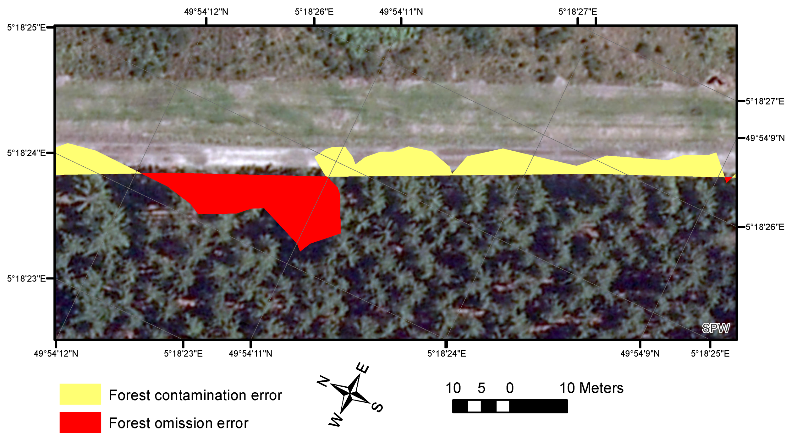
With respect to geometric precision, reference boundaries have been selected from correctly classified polygons in the homogeneous classes in order to avoid processing fuzzy boundaries during the quantitative assessment. The area of the omission and commission errors on both sides of the reference boundaries (Figure 5) is divided by the length of the reference boundary. The result provides an estimate of the mean distance to the boundaries. As shown in Table 6, those errors depend on the type of boundaries. Similar differences have been observed in previous studies [63].
9. Conclusions
The recommended good practices for GEOBIA quality assessment that were presented here are intending to extend the general guidelines from Olofsson et al. [4] in order to yield rigorous and defensible accuracy estimates in the case of GEOBIA. The objectives of the analysis should be clearly identified prior to the validation process in order to select the most appropriate approach. Critical choices include (i) the type of sampling unit (pixel or polygon), (ii) the types of accuracy indices (count-based or area-based) and (iii) the relevance of geometric quality assessment. GEOBIA accuracy assessment can be more complex than pixel-based accuracy assessment, but in turn provides more information such as area-dependent classification accuracy or class-specific boundary errors.
The proposed guidelines are based on arbitrary categories of GEOBIA objectives that are not exhaustive and not always exclusive. For instance, spatial entity detection and delineation could be combined in a single study. On the other hand, GEOBIA could also be used to derive quantitative parameters or class memberships that would require a specific validation framework. Furthermore, some key issues still need to be addressed in future studies. In order to further improve the accuracy assessment framework, standard methods for the quality assessment of boundaries are still needed and the impact of response design on the quality indices should be investigated. Furthermore, several indices proposed in this study still lack a formula for their variance, which is an issue for the comparison of algorithms and for the reporting of the estimated values. Last but not least, good practices for the estimation of areas based on GEOBIA wall-to-wall maps should be developed.
Acknowledgments
This research was conducted in the framework of the Lifewatch-Wallonia-Brussels project, funded by the Wallonia-Brussels Federation. The aerial image and the LIDAR dataset of the Walloon Region were kindly provided by the “Service Public de Wallonie” (License 160210-0951). Computational resources for the image processing have been partly provided by the “Consortium des Équipements de Calcul Intensif (CÉCI)”, funded by the “Fonds de la Recherche Scientifique de Belgique (F.R.S.-FNRS)” under Grant No. 2.5020.11. The authors also thank the attendees of the GEOBIA 2016 conference for inspiring discussions that took place. Last but not least, the authors thank the three reviewers for their valuable comments.
Author Contributions
The two authors equally contributed to this research.
Conflicts of Interest
The authors declare no conflict of interest. The founding sponsors had no role in the design of the study; in the collection, analyses or interpretation of data; in the writing of the manuscript; nor in the decision to publish the results.
Appendix A. Code Sample for the Response Design
def ResponseDesign(grass, crop, broadleaved, needleleaved, artificial, water, bare, shrub):
    vgt = grass + crop + broadleaved + needleleaved + shrub
    tot = grass + crop + broadleaved + needleleaved + artificial + water + bare + shrub
    forest = broadleaved + needleleaved
    if waterv > 0.5:
      return "water"
    elif artificial > 0.25:
      return "urban"
    elif vgt < 0.04:
      a = "bare⎵soil"
    elif vgt < 0.15:
      a = "sparse⎵vegetation"
    elif crop > 0.5 and (vgt-crop) >= 0.2:
      a= "vegetation⎵mixture⎵dominated⎵by⎵crops"
    elif cropv > 0.15 and (vgtv-cropv) >= 0.5 and for < 0.7:
      a= "vegetation⎵mixture⎵with⎵crops"
    elif grass > 0.5 and (forest + shrub) > 0.2:
      a = "vegetation⎵mixture⎵dominated⎵by⎵grass"
    elif grass > 0.15 and crop < grass and (forest + shrub) >= 0.5 and forest < 0.7:
      a= "vegetation⎵mixture⎵with⎵grass"
    elif crop > 0.15 and forest < crop and grass < crop:
      a = "cropland"
    elif grass > 0.150 and forest < grass and crop < grass:
      a = "grassland"
    elif forest > 0.150:
      if broadleaved > 0.25 and needleleaved > 0.25:
       a = "mixed⎵forest"
      elif broadleaved > needleleaved:
       a = "broadleaved⎵forest"
      else:
       a= "needleleaved⎵forest"
    elif shrub > 0.15:
         a = "shrubland"
    return a
Abbreviations
The following abbreviations are used in this manuscript:
| TP | True Positive |
| TN | True Negative |
| FN | False Negative |
| FP | False Positive |
| UA | User’s Accuracy |
| PA | Producer’s Accuracy |
| OA | Overall Accuracy |
| CE | Circular Error |
| CCP | Correctly Classified Polygons |
| NSP | Non-Sampled Polygons |
| LCCS | Land Cover Classification System |
| FAO | Food and Agriculture Organization |
| CI | Confidence Interval |
| RMSE | Root Mean Square Error |
| GEOBIA | Geographic Object-Based Image Analysis |
References
- Stehman, S.V.; Wickham, J.D. Pixels, blocks of pixels, and polygons: Choosing a spatial unit for thematic accuracy assessment. Remote Sens. Environ. 2011, 115, 3044–3055. [Google Scholar] [CrossRef]
- Castilla, C. We must pay more attention to rigor in accuracy assessment: Additional comment to The improvement of land cover classification by thermal remote sensing. Remote Sens. 2016, 288, 8–13. [Google Scholar]
- Strahler, A.H.; Boschetti, L.; Foody, G.M.; Friedl, M.A.; Hansen, M.C.; Herold, M.; Mayaux, P.; Morisette, J.T.; Stehman, S.V.; Woodcock, C.E. Global Land Cover Validation: Recommendations for Evaluation and Accuracy Assessment of Global Land Cover Maps. Available online: http://s3.amazonaws.com/academia.edu.documents/3461734/GOLD_25.pdf?AWSAccessKeyId=AKIAIWOWYYGZ2Y53UL3A&Expires=1497924032&Signature=CqruoCFfPw6KAFW%2FdTPdJ95ju40%3D&response-content-disposition=inline%3B%20filename%3DGlobal_land_cover_validation_Recommendat.pdf (accessed on 20 June 2017).
- Olofsson, P.; Foody, G.M.; Herold, M.; Stehman, S.V.; Woodcock, C.E.; Wulder, M.A. Good practices for estimating area and assessing accuracy of land change. Remote Sens. Environ. 2014, 148, 42–57. [Google Scholar] [CrossRef]
- Hernando Gallego, A.; Castilla Castellano, G.; Zang, C.; Mazumdar, D.; Macdermic, G. An Integrated Framework for Assessing the Accuracy of Geobia Landcover Products. Available online: http://oa.upm.es/21039/1/INVE_MEM_2012_129483.pdf (accessed on 20 June 2017).
- Burrough, P.A. Natural Objects with Indeterminate Boundaries. In Geographic Objects with Indeterminate Boundaries; Taylor & Francis: London, UK, 1996; Volume 2, pp. 3–28. [Google Scholar]
- Bian, L. Object-oriented representation of environmental phenomena: Is everything best represented as an object? Ann. Assoc. Am. Geogr. 2007, 97, 267–281. [Google Scholar] [CrossRef]
- Couclelis, H. Towards an operational typology of geographic entities with ill-defined boundaries. In Geographic Objects with Indeterminate Boundaries; Taylor & Francis: London, UK, 1996; pp. 45–55. [Google Scholar]
- Blaschke, T.; Hay, G.J.; Kelly, M.; Lang, S.; Hofmann, P.; Addink, E.; Feitosa, R.Q.; van der Meer, F.; van der Werff, H.; van Coillie, F.; et al. Geographic object-based image analysis–towards a new paradigm. ISPRS J. Photogramm. Remote Sens. 2014, 87, 180–191. [Google Scholar] [CrossRef] [PubMed]
- Hay, G.J.; Castilla, G. Geographic Object-Based Image Analysis (GEOBIA): A new name for a new discipline. In Object-Based Image Analysis; Springer: Berlin/Heidelberg, Germany, 2008; pp. 75–89. [Google Scholar]
- Baatz, M.; Schäpe, A. Multiresolution Segmentation: An optimization approach for high quality multi-scale image segmentation. In Angewandte Geographische Informationsverarbeitung XII; Strobl, J., Blaschke, T., Griesebner, G., Eds.; Salzburg Geographical Materials: Salzburg, Germany, 2000; pp. 12–23. [Google Scholar]
- Vetrivel, A.; Kerle, N.; Gerke, M.; Nex, F.; Vosselman, G. Towards automated satellite image segmentation and classification for assessing disaster damage using data-specific features with incremental learning. In Proceedings of the GEOBIA 2016: Solutions and Synergies, Enschede, The Netherlands, 14–16 September 2016. [Google Scholar]
- Girshick, R.; Donahue, J.; Darrell, T.; Malik, J. Rich feature hierarchies for accurate object detection and semantic segmentation. In Proceedings of the IEEE Conference on Computer Vision and Pattern Recognition, Columbus, OH, USA, 23–28 June 2014; pp. 580–587. [Google Scholar]
- Dean, A.; Smith, G. An evaluation of per-parcel land cover mapping using maximum likelihood class probabilities. Int. J. Remote Sens. 2003, 24, 2905–2920. [Google Scholar] [CrossRef]
- Smith, G.M.; Morton, R.D. Real world objects in GEOBIA through the exploitation of existing digital cartography and image segmentation. Photogramm. Eng. Remote Sens. 2010, 76, 163–171. [Google Scholar] [CrossRef]
- Castilla, G.; Hay, G. Image objects and geographic objects. In Object-Based Image Analysis; Springer: Berlin, Germany, 2008; pp. 91–110. [Google Scholar]
- Schöpfer, E.; Lang, S.; Albrecht, F. Object-fate analysis: Spatial relationships for the assessment of object transition and correspondence. In Object-Based Image Analysis; Springer: Berlin, Germany, 2008; pp. 785–801. [Google Scholar]
- Zhan, Q.; Molenaar, M.; Tempfli, K.; Shi, W. Quality assessment for geo-spatial objects derived from remotely sensed data. Int. J. Remote Sens. 2005, 26, 2953–2974. [Google Scholar] [CrossRef]
- Dronova, I.; Gong, P.; Wang, L. Object-based analysis and change detection of major wetland cover types and their classification uncertainty during the low water period at Poyang Lake, China. Remote Sens. Environ. 2011, 115, 3220–3236. [Google Scholar] [CrossRef]
- Whiteside, T.G.; Maier, S.W.; Boggs, G.S. Area-based and location-based validation of classified image objects. Int. J. Appl. Earth Obs. Geoinf. 2014, 28, 117–130. [Google Scholar] [CrossRef]
- Lizarazo, I. Accuracy assessment of object-based image classification: Another STEP. Int. J. Remote Sens. 2014, 35, 6135–6156. [Google Scholar] [CrossRef]
- Hernando, A.; Tiede, D.; Albrecht, F.; Lang, S. Spatial and thematic assessment of object-based forest stand delineation using an OFA-matrix. Int. J. Appl. Earth Obs. Geoinf. 2012, 19, 214–225. [Google Scholar] [CrossRef]
- Congalton, R.; Green, K. A practical look at the sources of confusion in error matrix generation. Photogramm. Eng. Remote Sens. 1993, 59, 641–644. [Google Scholar]
- Stehman, S. Selecting and Interpreting Measures of Thematic Classification Accuracy. Remote Sens. Environ. 1997, 62, 77–89. [Google Scholar] [CrossRef]
- Stehman, S.; Czaplewski, R. Design and analysis for thematic map accuracy assessment: Fundamental principles. Remote Sens. Environ. 1998, 64, 331–344. [Google Scholar] [CrossRef]
- Lamarche, C.; Santoro, M.; Bontemps, S.; d’Andrimont, R.; Radoux, J.; Giustarini, L.; Brockmann, C.; Wevers, J.; Defourny, P.; Arino, O. Compilation and Validation of SAR and Optical Data Products for a Complete and Global Map of Inland/Ocean Water Tailored to the Climate Modeling Community. Remote Sens. 2017, 9. [Google Scholar] [CrossRef]
- Congalton, R.G.; Green, K. Assessing the Accuracy of Remotely Sensed Data: Principles and Practices; CRC Press: Boca Raton, FL, USA, 2008. [Google Scholar]
- Eikvil, L.; Aurdal, L.; Koren, H. Classification-based vehicle detection in high-resolution satellite images. ISPRS J. Photogramm. Remote Sens. 2009, 64, 65–72. [Google Scholar] [CrossRef]
- Benz, U.C.; Hofmann, P.; Willhauck, G.; Lingenfelder, I.; Heynen, M. Multi-resolution, object-oriented fuzzy analysis of remote sensing data for GIS-ready information. ISPRS J. Photogramm. Remote Sens. 2004, 58, 239–258. [Google Scholar] [CrossRef]
- Gougeon, F.A. Automatic individual tree crown delineation using a valley-following algorithm and rule-based system. In Proceedings of the International Forum on Automated Interpretation of High Spatial Resolution Digital Imagery for Forestry, Victoria, BC, Canada, 10–12 February 1998; pp. 11–23. [Google Scholar]
- Yang, Z.; Wang, T.; Skidmore, A.; de Leeuw, J.; Said, M.; Freer, J. Spotting East African Mammals in Open Savannah from Space. PLoS ONE 2014, 9. [Google Scholar] [CrossRef] [PubMed]
- Van Coillie, F.; Van Camp, N.; De Wulf, R.; Bral, L.; Gautama, S. Segmentation quality evaluation for large scale mapping purposes in Flanders, Belgium. Available online: http://www.isprs.org/proceedings/XXXVIII/4-C7/pdf/VanCoillie_182.pdf (accessed on 20 June 2017).
- Da Costa, J.P.; Michelet, F.; Germain, C.; Lavialle, O.; Grenier, G. Delineation of vine parcels by segmentation of high resolution remote sensed images. Precis. Agric. 2007, 8, 95–110. [Google Scholar] [CrossRef]
- Montaghi, A.; Larsen, R.; Greve, M.H. Accuracy assessment measures for image segmentation goodness of the Land Parcel Identification System (LPIS) in Denmark. Remote Sens. Lett. 2013, 4, 946–955. [Google Scholar] [CrossRef]
- Stuckens, J.; Coppin, P.; Bauer, M. Integrating contextual information with per-pixel classification for improved land cover classification. Remote Sens. Environ. 2000, 71, 282–296. [Google Scholar] [CrossRef]
- Duro, D.C.; Franklin, S.E.; Dubé, M.G. A comparison of pixel-based and object-based image analysis with selected machine learning algorithms for the classification of agricultural landscapes using SPOT-5 HRG imagery. Remote Sens. Environ. 2012, 118, 259–272. [Google Scholar] [CrossRef]
- De Wit, A.; Clevers, J. Efficiency and accuracy of per-field classification for operational crop mapping. Int. J. Remote Sens. 2004, 25, 4091–4112. [Google Scholar] [CrossRef]
- Powers, D.M. Evaluation: From Precision, Recall and F-Measure to ROC, Informedness, Markedness and Correlation. Available online: https://www.researchgate.net/publication/276412348_Evaluation_From_precision_recall_and_F-measure_to_ROC_informedness_markedness_correlation (accessed on 20 June 2017).
- Ke, Y.; Quackenbush, L.J. A review of methods for automatic individual tree-crown detection and delineation from passive remote sensing. Int. J. Remote Sens. 2011, 32, 4725–4747. [Google Scholar] [CrossRef]
- Lamar, W.R.; McGraw, J.B.; Warner, T.A. Multitemporal censusing of a population of eastern hemlock (Tsuga canadensis L.) from remotely sensed imagery using an automated segmentation and reconciliation procedure. Remote Sens. Environ. 2005, 94, 133–143. [Google Scholar] [CrossRef]
- Liu, C.; Frazier, P.; Kumar, L. Comparative assessment of the measures of thematic classification accuracy. Remote Sens. Environ. 2007, 107, 606–616. [Google Scholar] [CrossRef]
- Radoux, J.; Bogaert, P. Accounting for the area of polygon sampling units for the prediction of primary accuracy assessment indices. Remote Sens. Environ. 2014, 142, 9–19. [Google Scholar] [CrossRef]
- Castilla, G.; Hernando, A.; Zhang, C.; McDermid, G.J. The impact of object size on the thematic accuracy of landcover maps. Int. J. Remote Sens. 2014, 35, 1029–1037. [Google Scholar] [CrossRef]
- Radoux, J.; Bogaert, P.; Fasbender, D.; Defourny, P. Thematic accuracy assessment of geographic object-based image classification. Int. J. Geogr. Inf. Sci. 2011, 25, 1365–8816. [Google Scholar] [CrossRef]
- MacLean, M.G.; Congalton, R.G. Map accuracy assessment issues when using an object-oriented approach. In Proceedings of the Annual Conference of the American Society for Photogrammetry and Remote Sensing, Sacramento, CA, USA, 19–23 March 2012; pp. 1–5. [Google Scholar]
- Lang, S.; Langanke, T. Object-based mapping and object-relationship modeling for land use classes and habitats. Photogramm. Fernerkund. Geoinf. 2006, 2006, 5–18. [Google Scholar]
- Tiede, D.; Lang, S.; Albrecht, F.; Hölbling, D. Object-based class modeling for cadastre-constrained delineation of geo-objects. Photogramm. Eng. Remote Sens. 2010, 76, 193–202. [Google Scholar] [CrossRef]
- Di Gregorio, A.; Jansen, L. Land Cover Classification System (LCCS): Classification Concepts and User Manual; Food and Agriculture Organization: Rome, Italy, 2000. [Google Scholar]
- Quintero, R.; Guzmán, G.; Menchaca-Mendez, R.; Torres, M.; Moreno-Ibarra, M. An ontology-driven approach for the extraction and description of geographic objects contained in raster spatial data. Expert Syst. Appl. 2012, 39, 9008–9020. [Google Scholar] [CrossRef]
- Worboys, M.F.; Hearnshaw, H.M.; Maguire, D.J. Object-oriented data modelling for spatial databases. Int. J. Geogr. Inf. Syst. 1990, 4, 369–383. [Google Scholar] [CrossRef]
- Radoux, J.; Defourny, P. Automated Image-to-Map Discrepancy Detection using Iterative Trimming. Photogramm. Eng. Remote Sens. 2010, 76, 173–181. [Google Scholar] [CrossRef]
- Card, D.H. Using known map category marginal frequencies to improve estimates of thematic map accuracy. Photogramm. Eng. Remote Sens. 1982, 48, 431–439. [Google Scholar]
- Tiede, D.; Lang, S.; Hoffmann, C. Domain-specific class modelling for one-level representation of single trees. In Object-Based Image Analysis; Springer: Berlin, Germany, 2008; pp. 133–151. [Google Scholar]
- Mesner, N.; Oštir, K. Investigating the impact of spatial and spectral resolution of satellite images on segmentation quality. J. Appl. Remote Sens. 2014, 8. [Google Scholar] [CrossRef]
- Ma, L.; Cheng, L.; Li, M.; Liu, Y.; Ma, X. Training set size, scale, and features in geographic object-based image analysis of very high resolution unmanned aerial vehicle imagery. ISPRS J. Photogramm. Remote Sens. 2015, 102, 14–27. [Google Scholar] [CrossRef]
- Grenier, M.; Labrecque, S.; Benoit, M.; Allard, M. Accuracy assessment method for wetland object-based classification. In Proceedings of the GEOBIA, Calgary, AB, Canada, 21 August 2008; pp. 285–289. [Google Scholar]
- Lang, S.; Zeil, P.; Kienberger, S.; Tiede, D. Geons–policy-relevant geo-objects for monitoring high-level indicators. In Proceedings of the GI Forum, Salzburg, Austria, 1–4 July 2008; Volume 8, pp. 180–185. [Google Scholar]
- Clinton, N.; Holt, A.; Scarborough, J.; Yan, L.; Gong, P. Accuracy assessment measures for object-based image segmentation goodness. Photogramm. Eng. Remote Sens. 2010, 76, 289–299. [Google Scholar] [CrossRef]
- Van Coillie, F.M.; Gardin, S.; Anseel, F.; Duyck, W.; Verbeke, L.P.; De Wulf, R.R. Variability of operator performance in remote-sensing image interpretation: The importance of human and external factors. Int. J. Remote Sens. 2014, 35, 754–778. [Google Scholar] [CrossRef]
- Albrecht, F.; Lang, S.; Hölbling, D. Spatial accuracy assessment of object boundaries for object-based image analysis. In Proceedings of the The International Archives of the Photogrammetry, Remote Sensing and Spatial Information Science, Ghent, Belgium, 29 June–2 July 2010. [Google Scholar]
- Greenwalt, C.R.; Schultz, M. Principles of Error Theory and Cartographic Applications. Available online: http://earth-info.nga.mil/GandG/publications/tr96.pdf (accessed on 20 June 2017).
- Tatem, A.J.; Noor, A.M.; Hay, S.I. Assessing the accuracy of satellite derived global and national urban maps in Kenya. Remote Sens. Environ. 2005, 96, 87–97. [Google Scholar] [CrossRef] [PubMed]
- Radoux, J.; Defourny, P. A quantitative assessment of boundaries in automated forest stand delineation using very high resolution imagery. Remote Sens. Environ. 2007, 110, 468–475. [Google Scholar] [CrossRef]
- Radoux, J.; Defourny, P. Quality assessment of segmentation results devoted to object-based classification. In Object-Based Image Analysis; Springer: Berlin, Germany, 2008; pp. 257–271. [Google Scholar]
- Persello, C.; Bruzzone, L. A novel protocol for accuracy assessment in classification of very high resolution images. IEEE Trans. Geosci. Remote Sens. 2010, 48, 1232–1244. [Google Scholar] [CrossRef]
Figure 1.
Illustration of the conceptual models for a Mediterranean forest in the South of France. In this landscape covered by an Ikonos image, trees are spatial entities that can be individually detected (stars on the left image). In the center, automated image segmentation creates spatial regions that correspond to the old firebreak and the undisturbed forest composed of trees, shrub and herbaceous vegetation. On the right, a continuous field representation highlights the lower (darker gray) vegetation density in the old firebreak.

Figure 2.
Illustration of the differences between area- and count-based accuracies for geo-objects, where correctly classified cells are in green and incorrect ones are in red (connected cells are part of a single spatial entity). The three synthetic examples have the same area-based accuracy (33% of the surface is misclassified), but different count-based accuracies. On the left, the three geo-objects have the same area, therefore area-based and count-based accuracies are identical. In the center, there is one large and one small geo-object: the size of the misclassified geo-object has an impact on the area-based accuracy, but not on the count-based accuracy. On the right, each geo-object is correctly detected (based on a majority rule), but there are segmentation errors. The area-based accuracy is then smaller than the count-based accuracy.

Figure 3.
Different legends applied on the same landscape. The central image is a pixel-based representation with a majority-rule legend. Two other representations are built consistently with this classification. On the left, the classes are based on a set of thresholds derived from LCCS-like rules. On the right, a majority-based legend is used. The extent of the urban area is largely affected depending on the chosen type of legend, and this has to be taken into account for the response design.

Figure 4.
Illustration of region-based sampling for the validation of spatial entities detection. Reference data were collected for eight randomly selected cells and compared with the detected entities. True positives are colored in green, false positives in red and false negatives in black. The grey points have not been validated.
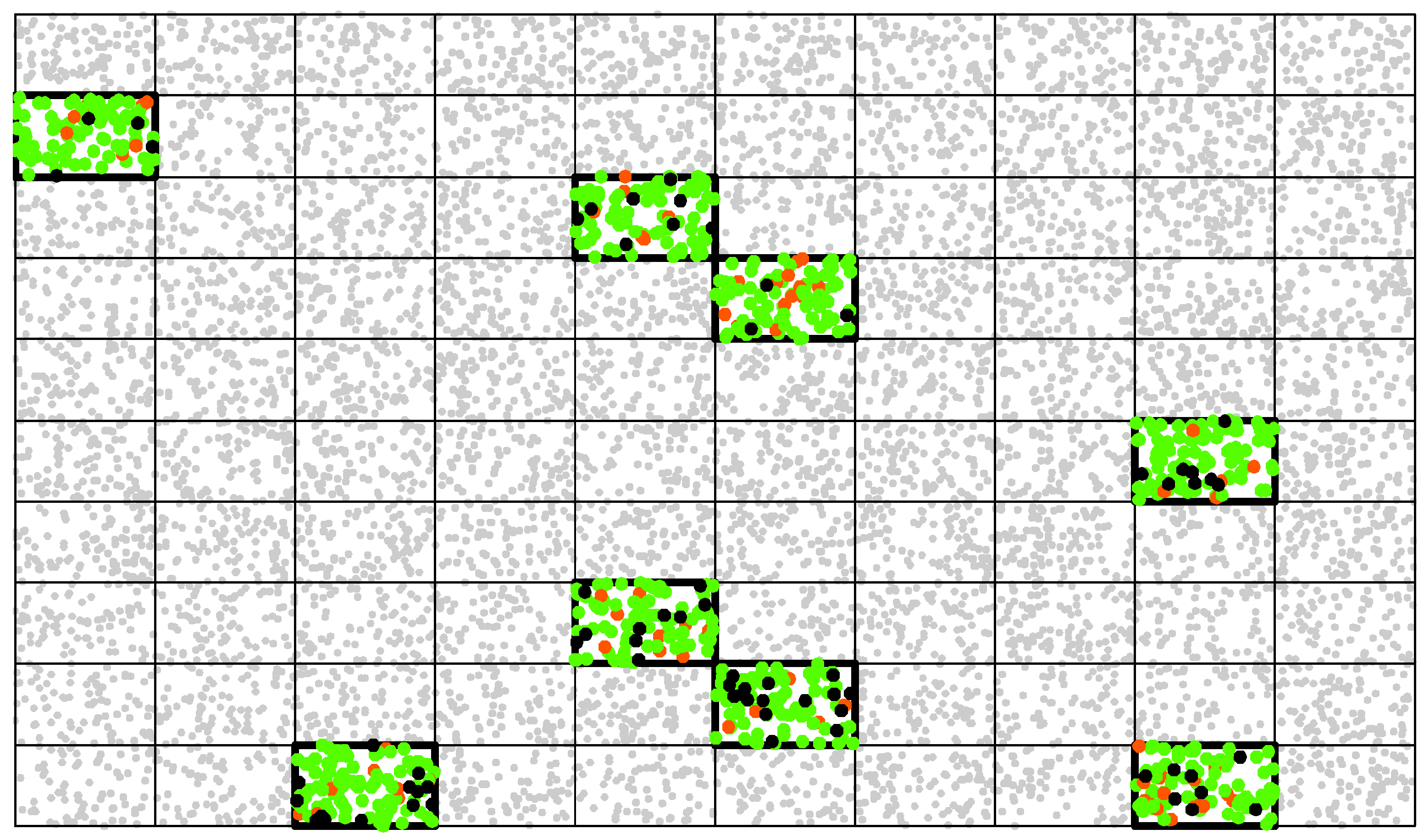
Figure 5.
Illustration of the segmentation errors along the boundaries. The highlighted polygons indicate mismatch with the boundaries of the reference polygons.
Figure 5.
Illustration of the segmentation errors along the boundaries. The highlighted polygons indicate mismatch with the boundaries of the reference polygons.

Table 1.
Recommended validation practices for four objectives of geographic object-based image analysis. The sign − indicates that indices are not necessary and + indicates that they are important. The sign ± indicates that the decision depends on multiple factors.
Table 1.
Recommended validation practices for four objectives of geographic object-based image analysis. The sign − indicates that indices are not necessary and + indicates that they are important. The sign ± indicates that the decision depends on multiple factors.
| Indices Section 3 | Sampling Unit Section 4 | Boundaries Section 6.2 | Structure Section 6.1 | |
|---|---|---|---|---|
| Enhanced pixel classification | Area-based | Pixels | − | − |
| Wall-to-wall (region) mapping | Area-based | Polygons | + | ± |
| Entities detection | Count-based | Polygons | − | ± |
| Entities delineation | (Count-based) | Polygons | + | + |
Table 2.
Characteristics of the strata used for the stratified sampling.
| Strata | Number of Polygons | Proportion of the Total Area | Average Polygon Size (ha) |
|---|---|---|---|
| Open areas | 470,731 | 0.463 | 1.5 |
| Forest areas | 363,804 | 0.331 | 1.3 |
| Others | 391,722 | 0.205 | 0.9 |
Table 3.
Area-based overall accuracy values for each stratum. CCP are the Correctly Classified Polygons in the sample according to the response design. NSP are the Non-Sampled Polygons. OA is the Overall Accuracy for each stratum.
Table 3.
Area-based overall accuracy values for each stratum. CCP are the Correctly Classified Polygons in the sample according to the response design. NSP are the Non-Sampled Polygons. OA is the Overall Accuracy for each stratum.
| Strata | Count of CCP | Area of CCP | Area of NSP | OA (%) |
|---|---|---|---|---|
| Open areas | 345 | 600 ha | 785,294 ha | 90.9 |
| Forest areas | 185 | 267 ha | 562,135 ha | 84.5 |
| Others | 123 | 112 ha | 347,005 ha | 88.6 |
Table 4.
Count-based confusion matrix. The LCCS-based legend includes six homogeneous classes as well as associations of different entities from larger scale. The homogeneous classes are Cropland (C), Broadleaved Forest (BLF), Needle-Leaved Forest (NLF), Grassland (G), Bare soils (B) and Water (W). Heterogeneous classes include Urban areas (U), Sparse Vegetation (SV), Crop-dominated vegetation Mixture (CM1), Mixture of vegetation with Crops (CM2), Tree-dominated vegetation mixture without crops (TM1) and open vegetation mixture with some trees (TM2). The table also includes the Count-based Users’ () and Producers’ Accuracies (). The values in this table were not weighted by their sampling probability for the sake of clarity, but the relative number of polygons in each stratum is taken into account for the computation of the producers’ accuracy.
| Class | C | CM1 | CM2 | BLF | NLF | MF | TM1 | TM2 | G | SV | U | B | W | |
|---|---|---|---|---|---|---|---|---|---|---|---|---|---|---|
| C | 143 | 5 | 1 | 0 | 0 | 0 | 0 | 2 | 7 | 0 | 0 | 1 | 1 | 0.89 |
| CM1 | 3 | 11 | 1 | 0 | 0 | 0 | 0 | 0 | 1 | 0 | 0 | 0 | 0 | 0.69 |
| CM2 | 1 | 1 | 23 | 0 | 0 | 0 | 1 | 2 | 8 | 0 | 2 | 0 | 0 | 0.60 |
| BLF | 0 | 0 | 1 | 107 | 0 | 7 | 5 | 4 | 0 | 0 | 0 | 0 | 1 | 0.86 |
| NLF | 0 | 0 | 0 | 1 | 45 | 0 | 0 | 0 | 0 | 0 | 0 | 0 | 0 | 0.98 |
| MF | 0 | 0 | 0 | 2 | 2 | 15 | 1 | 0 | 0 | 0 | 0 | 0 | 0 | 0.75 |
| TM1 | 0 | 0 | 0 | 1 | 0 | 1 | 21 | 1 | 0 | 0 | 0 | 0 | 0 | 0.87 |
| TM2 | 0 | 0 | 1 | 0 | 0 | 0 | 2 | 9 | 1 | 0 | 0 | 0 | 0 | 0.69 |
| G | 3 | 0 | 0 | 0 | 0 | 0 | 3 | 8 | 229 | 1 | 0 | 4 | 0 | 0.92 |
| SV | 0 | 0 | 0 | 0 | 0 | 0 | 0 | 0 | 0 | 2 | 0 | 0 | 0 | 1.00 |
| U | 0 | 0 | 0 | 0 | 0 | 0 | 0 | 0 | 0 | 0 | 45 | 2 | 0 | 0.96 |
| B | 0 | 0 | 0 | 0 | 0 | 0 | 0 | 0 | 0 | 0 | 0 | 1 | 0 | 1.00 |
| W | 0 | 0 | 0 | 0 | 0 | 0 | 0 | 0 | 0 | 0 | 0 | 0 | 6 | 1.00 |
| 0.95 | 0.65 | 0.91 | 0.96 | 0.96 | 0.68 | 0.74 | 0.33 | 0.93 | 0.62 | 0.95 | 0.11 | 0.72 |
Table 5.
Area-based confusion matrix. The LCCS-based legend includes six homogeneous classes as well as associations of different entities from larger scale. The homogeneous classes are Cropland (C), Broadleaved Forest (BLF), Needle-Leaved Forest (NLF), Grassland (G), Bare soils (B) and Water (W). Heterogeneous classes include Urban areas (U), Sparse Vegetation (SV), Crop-dominated vegetation Mixture (CM1), Mixture of vegetation with Crops (CM2), Tree-dominated vegetation mixture without crops (TM1) and open vegetation mixture with some trees (TM2). The table also includes the Count-based Users’ () and Producers’ Accuracies (). The values in this table were not weighted by their sampling probability for the sake of clarity, but the relative number of polygons in each stratum is taken into account for the computation of the producers’ accuracy.
| Class | C | CM1 | CM2 | BLF | NLF | MF | TM1 | TM2 | G | SV | U | B | W | |
|---|---|---|---|---|---|---|---|---|---|---|---|---|---|---|
| C | 301 | 7 | 0.4 | 0 | 0 | 0 | 0 | 4 | 6 | 0 | 0 | 0.9 | 0.5 | 0.94 |
| CM1 | 3 | 7 | 0.2 | 0 | 0 | 0 | 0 | 0 | 0.3 | 0 | 0 | 0 | 0 | 0.66 |
| CM2 | 0.3 | 0.2 | 22 | 0 | 0 | 0 | 1 | 4 | 6 | 0 | 2 | 0 | 0 | 0.65 |
| BLF | 0 | 0 | 0.5 | 122 | 0 | 9 | 4 | 9 | 0 | 0 | 0 | 0 | 0.2 | 0.84 |
| NLF | 0 | 0 | 0 | 2 | 78 | 0 | 0 | 0 | 0 | 0 | 0 | 0 | 0 | 0.97 |
| MF | 0 | 0 | 0 | 0.7 | 2 | 15 | 0.5 | 0 | 0 | 0 | 0 | 0 | 0 | 0.81 |
| TM1 | 0 | 0 | 0 | 1 | 0 | 1 | 21 | 1 | 0 | 0 | 0 | 0 | 0 | 0.87 |
| TM2 | 0 | 0 | 0.6 | 0 | 0 | 0 | 2 | 7 | 0.6 | 0 | 0 | 0 | 0 | 0.69 |
| G | 5 | 0 | 0 | 0 | 0 | 0 | 5 | 6 | 338 | 0.8 | 0 | 3 | 0 | 0.90 |
| SV | 0 | 0 | 0 | 0 | 0 | 0 | 0 | 0 | 0 | 2 | 0 | 0 | 0 | 1.00 |
| U | 0 | 0 | 0 | 0 | 0 | 0 | 0 | 0 | 0 | 0 | 36 | 1 | 0 | 0.94 |
| B | 0 | 0 | 0 | 0 | 0 | 0 | 0 | 0 | 0 | 0 | 0 | 0.5 | 0 | 1.00 |
| W | 0 | 0 | 0 | 0 | 0 | 0 | 0 | 0 | 0 | 0 | 0 | 0 | 7 | 1.00 |
| 0.95 | 0.66 | 0.89 | 0.96 | 0.96 | 0.68 | 0.74 | 0.22 | 0.94 | 0.47 | 0.98 | 0.05 | 0.87 |
Table 6.
Geometric errors along the boundaries for the main homogeneous classes.
| Type of Boundaries | Mean Absolute Error | Maximum Error |
|---|---|---|
| Crop and pasture | 2 m | 6 m |
| Broadleaved forest and open areas | 3.5 m | 15 m |
| Needle-leaved forest and open areas | 2.5 m | 13 m |
| Water and open areas | 1 m | 2 m |
© 2017 by the authors. Licensee MDPI, Basel, Switzerland. This article is an open access article distributed under the terms and conditions of the Creative Commons Attribution (CC BY) license (http://creativecommons.org/licenses/by/4.0/).
Share and Cite
MDPI and ACS Style
Radoux, J.; Bogaert, P. Good Practices for Object-Based Accuracy Assessment. Remote Sens. 2017, 9, 646. https://doi.org/10.3390/rs9070646
AMA Style
Radoux J, Bogaert P. Good Practices for Object-Based Accuracy Assessment. Remote Sensing. 2017; 9(7):646. https://doi.org/10.3390/rs9070646
Chicago/Turabian StyleRadoux, Julien, and Patrick Bogaert. 2017. "Good Practices for Object-Based Accuracy Assessment" Remote Sensing 9, no. 7: 646. https://doi.org/10.3390/rs9070646
Note that from the first issue of 2016, this journal uses article numbers instead of page numbers. See further details here.