
Circular Regression Applied to GNSS-R Phase Altimetry
by
 and
and
Jean-Christophe Kucwaj
*, 
Serge Reboul
*,
Georges Stienne
*,
Jean-Bernard Choquel
and
Mohammed Benjelloun
Laboratoire d’Informatique, Signal et Image de la Côte d’Opale (LISIC, EA 4491), Université du Littoral Côte d’Opale (ULCO), F-62228 Calais, France
*
Authors to whom correspondence should be addressed.
Remote Sens. 2017, 9(7), 651; https://doi.org/10.3390/rs9070651
Submission received: 5 May 2017
/
Revised: 15 June 2017
/
Accepted: 20 June 2017
/
Published: 23 June 2017
(This article belongs to the Section Ocean Remote Sensing)
Abstract
:This article is dedicated to the design of a linear-circular regression technique and to its application to ground-based GNSS-Reflectometry (GNSS-R) altimetry. The altimetric estimation is based on the observation of the phase delay between a GNSS signal sensed directly and after a reflection off of the Earth’s surface. This delay evolves linearly with the sine of the emitting satellite elevation, with a slope proportional to the height between the reflecting surface and the receiving antenna. However, GNSS-R phase delay observations are angular and affected by a noise assumed to follow the von Mises distribution. In order to estimate the phase delay slope, a linear-circular regression estimator is thus defined in the maximum likelihood sense. The proposed estimator is able to fuse phase observations obtained from several satellite signals. Moreover, unlike the usual unwrapping approach, the proposed estimator allows the sea-surface height to be estimated from datasets with large data gaps. The proposed regression technique and altimeter performances are studied theoretically, with further assessment on both synthetic and real data.
1. Introduction
Global Navigation Satellite Systems-Reflectometry (GNSS-R) is a passive bi-static radar technique for Earth observation using GNSS signals as signals of opportunity. This remote sensing technique uses the L-band signal coming directly from a GNSS satellite and the signal reflected by the Earth in order to characterize the reflecting surface. Several applications have been developed, such as ocean altimetry [1], the characterization of sea surface roughness [2] and soil moisture estimation [3]. Using GNSS signals for Earth observation offers multiple advantages: precision of the location and dating of the retrieved data, low sensibility to atmospheric perturbations and global coverage by several existing constellations, implying the availability of numerous reflections observations at the same time. In this work, the application concerns the design of a low altitude GNSS radar system for altimetry of water surfaces in coastal areas.
The altimetry measurement is derived from the path difference between the direct and reflected signals. This path difference can be estimated from the carrier-to-noise ratio observations [4,5,6,7,8], the code observations [9,10,11,12,13,14] or the phase observations [15,16]. The GNSS signal path can be measured with the observation of phase delay between the direct and reflected signals. This phase delay provides a range measurement with an ambiguity corresponding to the signal wavelength. Many methods are proposed in the published works to solve this ambiguity [14,17]. Ambiguity resolution is a complicated problem that is still studied nowadays. The technique developed in this article allows this problem to be skipped. The phase difference between the direct and the reflected signals evolves linearly with the satellite elevation sine [18,19]. The slope of this evolution provides an observation of the height between the receiving antennas and the reflecting surface. In this article, we observe the phase difference with a receiver similar to the one proposed in [20]. The phase delay is obtained by correlating the reflected signal and a clean replica of the direct signal [19,21]. This approach can be considered as conventional GNSS-R (cGNSS-R) with master/slave channel configuration [18,22].
The observations of phase delay are noisy. In the published works, long coherent integration [23] and phase unwrapping are used in order to improve the estimation process. In [23,24], a linear interpolation of the unwrapped phase is used to derive an accurate estimate of the height. In [19], an iterative unwrapping circular technique is proposed. This approach aims at improving the unwrapping process by smoothing the angular observations with a circular fusion filter. None of these methods can be used in the case of sets of measurements including long data losses.
Unlike the code measurements, the carrier phase measurements are angular data. Angular data are defined in an interval of length ( or ), which corresponds, in terms of range, to the wavelength of the observed GNSS signal [25,26]. Consequently, the classical estimation techniques of the linear domain provide biased results for circular data due to the occurrence of transitions between the interval bounds over time. In this context, techniques defined in the linear domain (for example, using the Gaussian distribution) are inapplicable for statistical processing.
It was shown in [27] that the additive noise on the phase delay of a GNSS signal follows a von Mises distribution. This distribution (also called circular normal distribution) is widely used for the modeling of angles in a Bayesian framework [28,29]. Applied to angular observations, the von Mises distribution plays the same role as the normal distribution for observations defined on the line. Detailed overviews of circular statistics can be found in [30,31,32]. In recent years, several techniques, based on periodic distributions, have been defined for the statistical processing of circular signals. For example, using a von Mises distribution, a circular median filter is defined in [33] and applied to color images processing. The same distribution is used to derive a circular recursive filter (or Kalman-like filter) for angle measurements in [34]. In the context of dynamic estimation, a circular filter was proposed for GNSS phase smoothing in [35] and GNSS phase positioning with cycle slip detection and repair in [35]. In [36], a von Mises-based Probability Hypothesis Densities (PHD) filter is proposed and applied to the problem of multiple angular targets tracking. In [37], it is the Bingham distribution that is used for deriving a recursive filter dedicated to symmetric circular problems. The optimality of such estimation techniques according to various circular error criteria and further techniques for reaching such optimality have been investigated in [38,39].
In this article, using the von Mises distribution, we propose to define the maximum likelihood estimator that provides a direct estimation of the height with observations defined in the circular domain. The proposed estimator is defined as a linear-circular regression [30,40] in the time reference frame of the sine of the satellite elevation and allows one to avoid the phase unwrapping step. It is based on a loss function derived from the measurement likelihood. This loss function is maximized using a Newton–Raphson algorithm.
2. GNSS-R Altimetry Using Phase Measurement
2.1. Height Retrieval Using GNSS Phase Signals
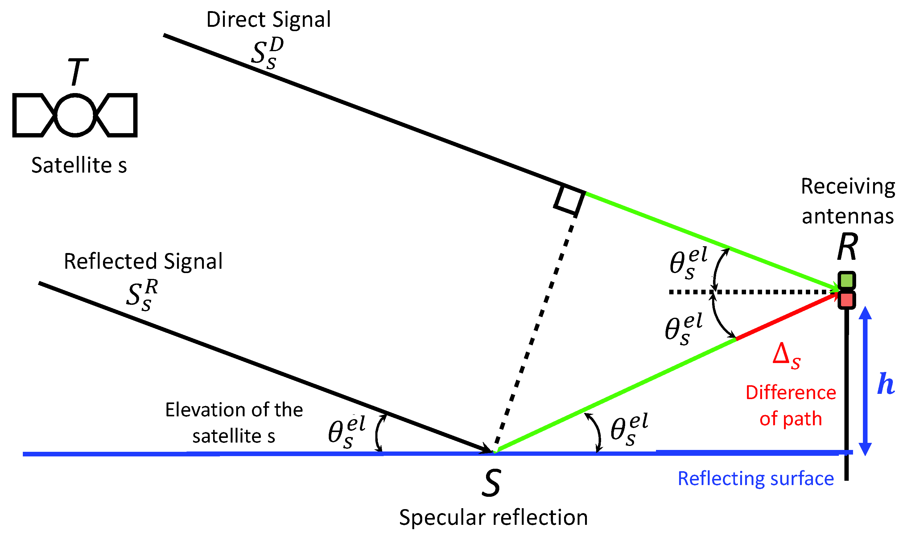
Figure 1 describes the geometry of the GNSS-R altimeter. In this figure, T is the transmitting GNSS satellite and S is the specular reflection point. In our approach, the surface of reflection is assumed to be the plane, and the incidence and reflection angles are the same. R is the position of the receiving antennas, at an altitude h over the reflecting surface. Two antennas are considered: an up-looking antenna, with right-hand circular polarization, and a down-looking antenna, with left-hand circular polarization. These two antennas respectively sense the direct and the reflected GNSS signal. The direct and reflected signals of the s-th satellite are respectively noted and . The elevation angle is . For a low altitude h, the satellite is assumed to be at an infinite distance in regards to the position of the receiver. Consequently, the elevation angle is equal to the incidence and the reflection angle.
The height h between the antennas and the reflecting surface is the parameter to estimate. The height is derived from the path difference between the direct and the reflected signals. According to the system geometry presented in Figure 1, the path difference for satellite s at instant t is given by the following equation:
where the satellite elevation can be derived from the current GNSS satellites ephemeris and from the GNSS positioning of the receiving antennas.
In the case of the civil component of a GPS-L1 signal received from the satellite s, the direct signal and the reflected signal can be defined as follows:
where and are the amplitudes of the direct and reflected signals. is the CDMA code broadcast by the satellite, at a period of one millisecond. is the code delay of the received signal at the RHCP (Right Hand Circular Polarization)antenna (in seconds). is the frequency of the direct signal, and is its phase delay. and are additive zero-mean white Gaussian noises [26], respectively, on the direct and reflected signals. is the path difference between the direct and the reflected signals for the satellite s. c is the speed of light. The term is the difference of phase between the direct and the reflected signals for satellite s.
The phase corresponding to the path difference observed in the phase delay can be derived from Equation (1) as:
is an angular datum, defined in an interval of length , which corresponds to cm in range for a GPS-L1 signal. We notice, from Equation (4) that evolves linearly with , the sine of the s-th satellite elevation. The slope of in the elevation sine time frame is proportional to the height h between the receiving antennas and the reflecting surface, with a factor of .
2.2. Phase Observation
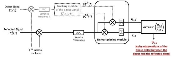
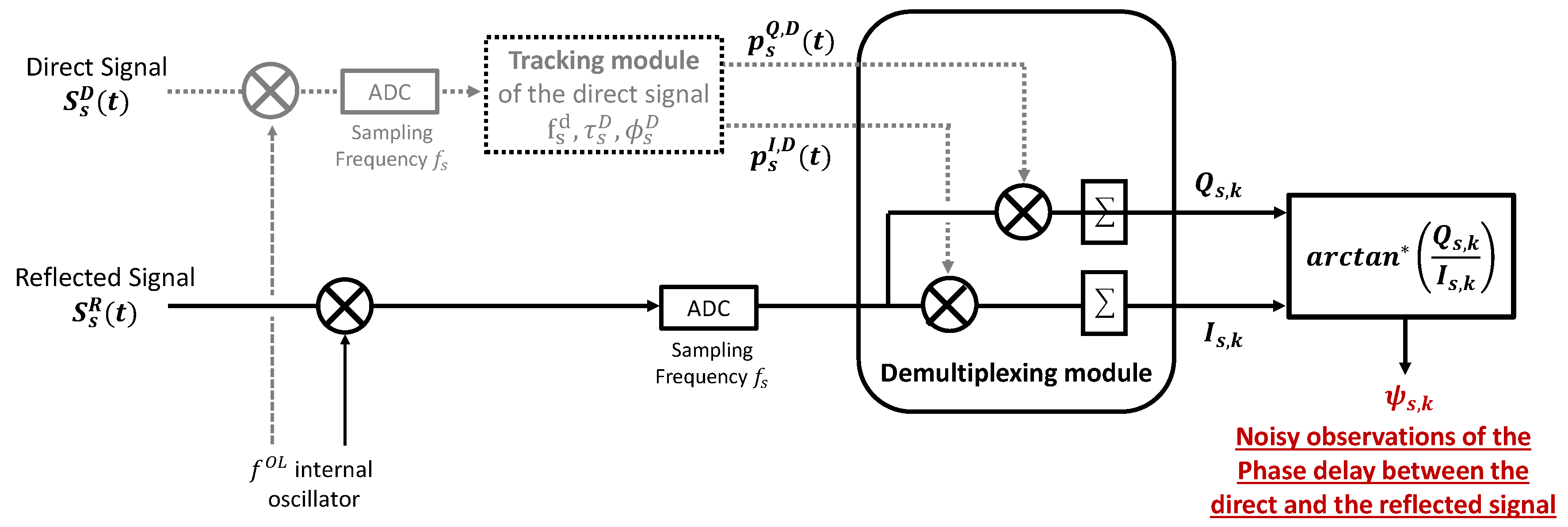
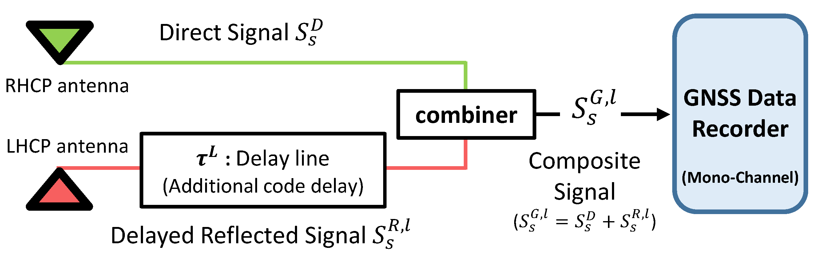
Figure 2 presents the different blocks of the receiver architecture used to observe the phase delay . This receiver architecture is designed as a master/slave configuration as in [18]. The incoming direct and reflected signals, respectively and , are demodulated with an internal oscillator at frequency and digitized with a sampling frequency . The local oscillator frequency is fixed so the residual frequency after down-conversion is both larger than the inverse of the integration interval and lower than half the sampling frequency . The tracking module of the direct signal provides the GNSS parameters , and in order to construct the replicas and . The demultiplexing module described in Figure 2 provides the observations and .
Let us define and as the in-phase and quadrature components at instant k for the s-th satellite. k is the measurement index, the measurements being separated by a fixed period corresponding to the coherent integration used in the tracking module. This period has a minimum value of ms, which corresponds to the C/A code length. These components are obtained after the demodulation of the reflected signal with local replicas of the direct signal:
where and are the in-phase and quadrature clean replicas of the direct signal. These local replicas are constructed with the parameters provided by the tracking loop of the direct signal.
These parameters are the estimates of , and . The local replicas are defined by:
Finally, and can be modeled as:
where models the normalized correlation function of the CDMA code. For ground-based measurements, we assume that the altitude of the receiving antennas is lower than 150 m, implying that is not null. and are two independent zero-mean Gaussian noises.
Using Relations (9) and (10), a noisy observation of the phase delay , also called interferometric phase observations [18] , can be obtained every millisecond with the following model:
where is the quadrant-specific arc-tangent and is a zero-mean noise. The noise is assumed to be distributed according to a von Mises distribution [27,30] with a concentration parameter . The noise on the observations of is not correlated over time as there is no tracking of the reflected signal. In this model, the height h and the concentration parameter are the only unknown parameters.
3. Linear-Circular Regression Applied to GNSS-R Altimetry
3.1. Circular Model
The normal distribution is inappropriate for a physical process involving periodic angle measurements. The von Mises distribution, also known as the circular normal distribution , describes a circular random variable and can be considered as the equivalent of the normal distribution in the circular domain [30].
The von Mises distribution for a circular random variable , with mean value and concentration parameter , is given by:
with:
The concentration parameter takes values between zero and infinity and approximately behaves like the inverse of the Gaussian variance. The term of normalization is the modified Bessel function of the first kind and order zero.
In this paper, we propose the following model for the observation of , the phase delay associated with the satellite s at instant k:
is the angular observation and the associated reference time frame. The parameters and are respectively the ordinate at the origin and the slope of the linear evolution of the observations. The term is a zero-mean additive von Mises noise realization with a concentration parameter . In our approach, the reference time frame corresponds to the sine of the elevation: , and the value of h is derived from the value of : .
3.2. Log-Likelihood Estimator
In order to estimate the two parameters and , we derive the likelihood function associated with the measurement model. The probability density function is given by:
Considering N measurements , the likelihood function is given by:
and the log-likelihood function is:
With the log-likelihood function, we define the following contrast function:
The values of and that maximize the contrast function provide the maximum likelihood estimates and .
is the solution of:
and finally, is obtained with the following expression:
This expression shows that can be directly deduced from the estimation of . We conclude that is the only parameter to estimate to fit the model to the observed data.
We propose to use the Newton–Raphson algorithm to estimate the value of the slope that maximizes . The Newton–Raphson algorithm is an iterative procedure based on the second derivative of the loss function :
where g is a step size. The estimate that maximizes the contrast function is obtained iteratively from Equations (18) and (21) with the following relations:
In this recursive scheme, converges to a local maximum of the contrast function .
In the GNSS-R altimetry context, the height is deduced from the estimated value of the slope by:
Assuming that all of the GNSS signal reflections are on the same surface, we can suppose that the slope is common for all of the phase delay evolutions corresponding to all of the satellites in view. All of the interferometric phase observations can be observed in the same time reference frame, and it is possible to construct a contrast function fusing several GNSS reflections. The contrast function can be modified from Relation (18) in order to take into account the whole set of S visible satellites. The loss function becomes:
The proposed height estimator is unchanged, replacing the sums from one to N by sums from one to .
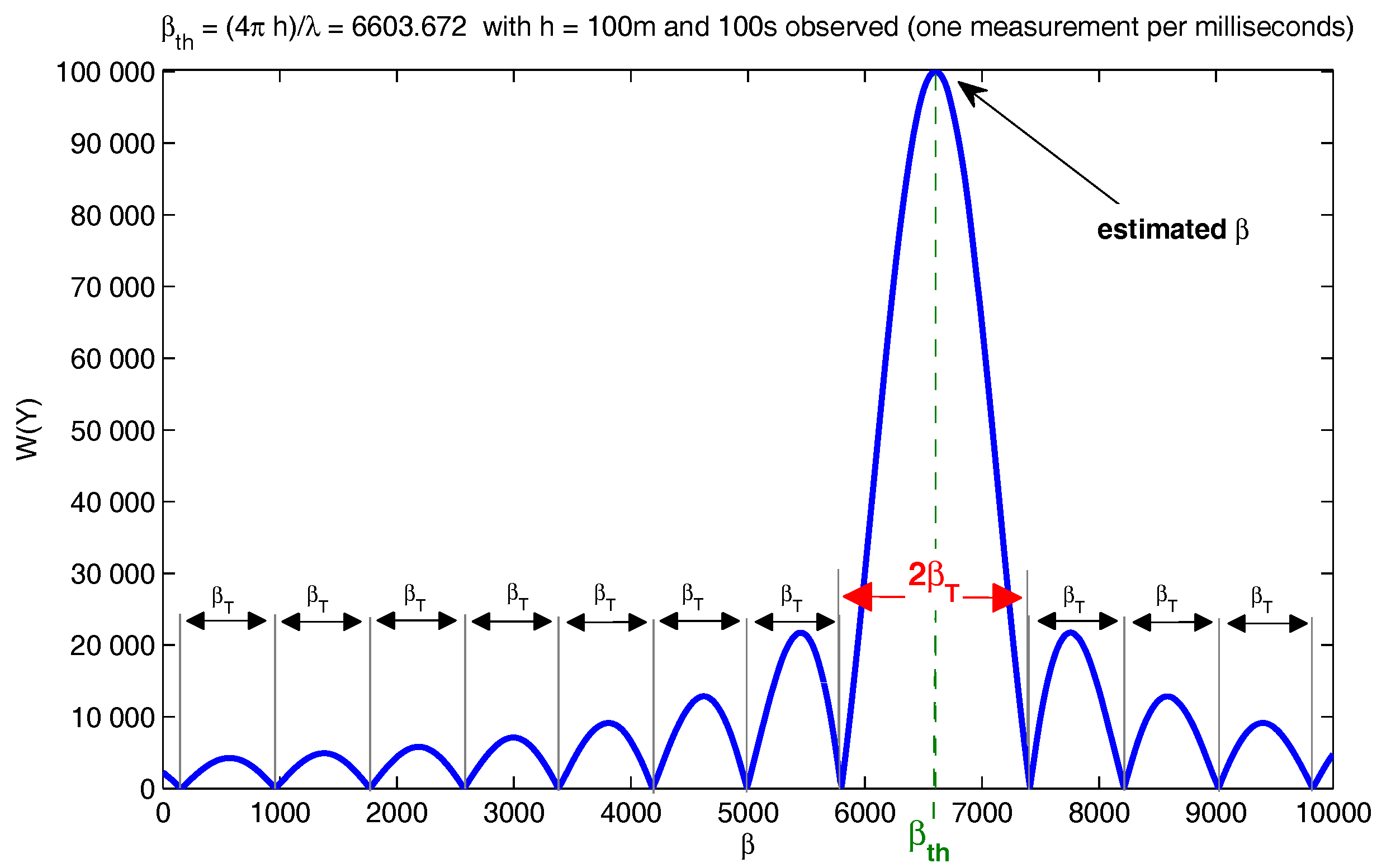
3.3. Initialization and Assessment
Figure 3 shows a theoretical representation of as a function of the slope . We observe that the contrast function has several local maxima and a global maximum corresponding to th, the value to estimate. The Newton–Raphson algorithm is a local maximization technique. The estimate thus depends on the initialization . In order to reach the global maximum, we propose to initialize with an additional search step.
Due to the periodicity of the angular data, the local maxima of are distributed periodically, with a period denoted . This period only depends on the parameter. The period can thus be obtained by numerically solving the following unnoisy formula, where the measurement component is canceled (which corresponds to th = 0):
which can be rewritten as:
where is the mean of .
The period can be obtained as the minimum value that solves this equation. , the initialization of the Newton–Raphson algorithm, can then be obtained by realizing a first fast global maximization of with a search step of .
The expected accuracy of the proposed method is the same as the variance of the classic linear regression. For our model, the theoretical variance of the estimate is:
The standard deviation of the noise is defined as in the linear domain by approximating the von Mises distribution by a wrapped normal distribution. It is shown in [30] that can be linked to using the following expression:
with the concentration parameter associated with the von Mises noise measurement of the observed phase delay.
We can observe in Expression (28) that the variance of the estimate decreases (so the accuracy of the estimation increases) when the denominator increases. The denominator increases as the data are observed over a larger span of satellite elevation. In practice, in order to increase this span, large observation durations are needed. This is a major drawback of the proposed method. However, we show that it is possible to fuse several reflections observations using the contrast function defined in Equation (25). In this case, the denominator of Expression (28), and the estimation accuracy, is increased by using GNSS satellites that have different elevations.
4. Experimentation
4.1. Assessment with Synthetic Data
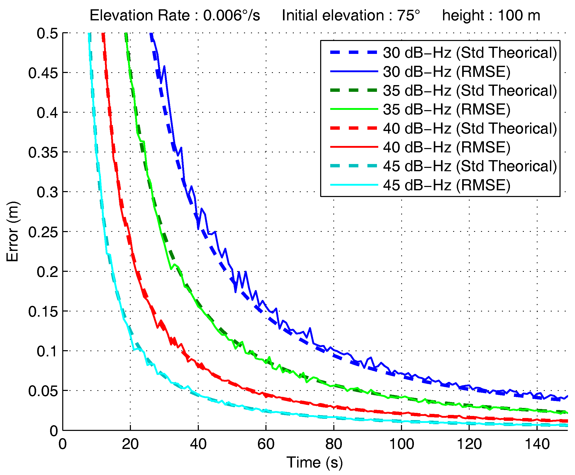
We first assess the linear-circular regression on synthetic GNSS-R data. In this section, we consider synthetic data corresponding to a realistic GPS constellation scenario. The height is fixed at 100 m ( 6603.63), and the observation rate is fixed at 1000 Hz (one measure per millisecond, the length of the GPS-L1 civil code) . The noise of the interferometric phase observations is defined for different values of carrier to noise ratio C/. The carrier to noise ratio and the associated concentration parameter are described in Table 1. In common conditions, the carrier to noise ratio associated with the interferometric signal is close to 40 dB-Hz for GPS-L1 signals, so we assess the estimator for values of 30, 35, 40 and 45 dB-Hz.
The interferometric phase observations are obtained with an initial elevation fixed at and an elevation rate of 0.006/s. This corresponds to a usual case as observed over the city of Calais [7,19]. We compute the RMSE (Root Mean Square Error) of the estimator over 300 realizations of the observations model. Figure 4 presents the obtained RMSE as a function of the integration time along with the theoretical standard deviation of the estimator, calculated using Equation (28).
We observe from Figure 4 that the RMSE fits the theoretical standard deviation. We first note that the linear-circular regression height estimator is unbiased (the mean error is indeed null, and the RMSE thus corresponds to the standard deviation of the estimator). We also can conclude that the theoretical formulation for the standard deviation is correct. Furthermore, we observe that the linear-circular regression height estimate reaches an accuracy of at least 5 cm for a period of integration of 100 s for any carrier to noise ratio superior to 35 dB-Hz. We also observe, as expected, that when the carrier to noise ratio increases, the accuracy of the estimator increases.
We show in Figure 5 the standard deviation of the proposed estimator as a function of the satellite elevation rate and for various initial elevations. For these simulations, the considered observation period is fixed at 100 s, and the is 35 dB-Hz. We observe that the standard deviation of the estimated height decreases when the elevation rate increases, as expected according to Equation (28). Figure 5 also depicts the influence of the initial elevation: the estimator is less precise for high initial elevations, with especially highly increasing precision losses for initial elevations increasing over . High values of the initial elevation indeed provide smaller spans as the sine gets very close to one for any elevation over .
4.2. Experimental Setup
In our implementation, we use an experimental setup that allows recording the direct and the reflected signals using only one channel receiver. This original setup is presented Figure 6. In the proposed setup, the reflected GNSS signal is delayed using a fiber optic coil. The delay, denoted , depends on the length of the coil and is known by the user. The reflected signal is summed with the direct signal before digitization using a signal combiner. The fiber optic coil does not affect the linear behavior of the phase delay. In our approach, the aim of this delay line is to separate the direct and the reflected signal in time in order to be able to track these two signals independently using a single channel receiver. Such a system is less complex and less expensive than a classical multi-channel data grabber for GNSS reflectometry and also requires less memory. However, the recording of both signals in a single channel reduces the by approximately 3 dB-Hz: the noise associated with the combination of satellite signals sensed affects the recorded reflected signal and vice versa.
The composite signal (sum of the direct and reflected GNSS signals) is recorded by a Syntony “SiFEn-R-one by one” data grabber. This front-end receiver has a sampling frequency up to 200 MHz and a quantization up to 8 bits. It can be used for any GNSS signal, with adjustable frequency down-conversion. For the experimentation, a sampling frequency of 25 MHz and a quantization of 1 bit were used. The down-conversion frequency is fixed for the frequency of the GPS-L1 band. The additional code delay is fixed at s (1 km of optical fiber), which is sufficient for separating the direct and reflected signals’ correlation peaks for a ground-based experiment with satellites at any observable elevation. Figure 7 presents a Delay-Doppler Mapping (DDM) of a composite signal sensed during the experimentations. The composite signal is processed using the architecture described in Figure 2. The additional delay is taken into account in the local code replica in Equations (7) and (8) by adding it to .
4.3. Assessment with Real Data
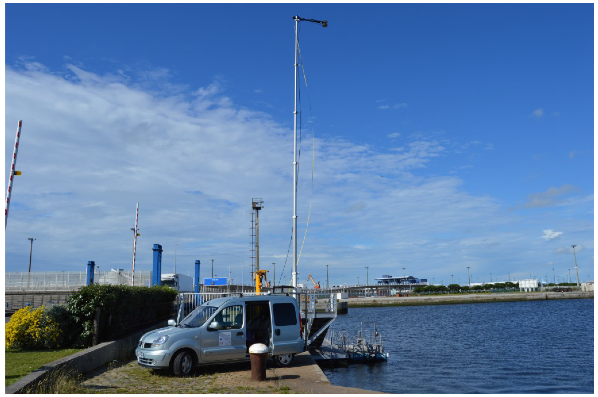
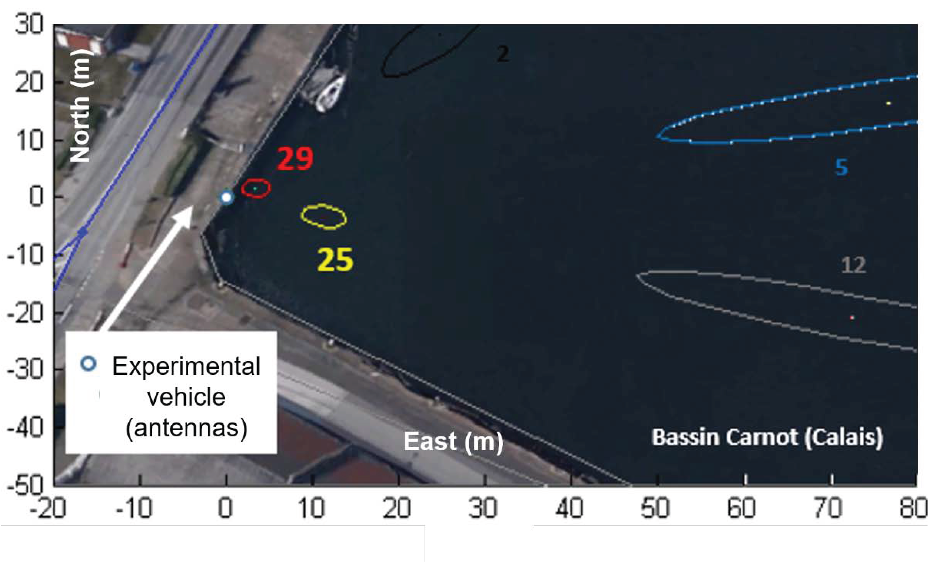
This experimentation on real data is an application of the experimental setup presented in the previous section, the receiver architecture described Section 2.2 and the circular estimator described Section 3.3. The proposed system is tested using the civil component of GPS-L1 signals reflected on an artificial canal basin in Calais. As shown Figure 8, the receiving antennas system, composed of an up-looking RHCP antenna and a down-looking LHCP (Left Hand Circular Polarization)antenna, is located at the top of a telescopic mast. The mast can rise up to a height of 10 m and is mounted on an experimental vehicle. The reference height between the reflecting water surface and the receiving antennas is obtained using a measurement tape.
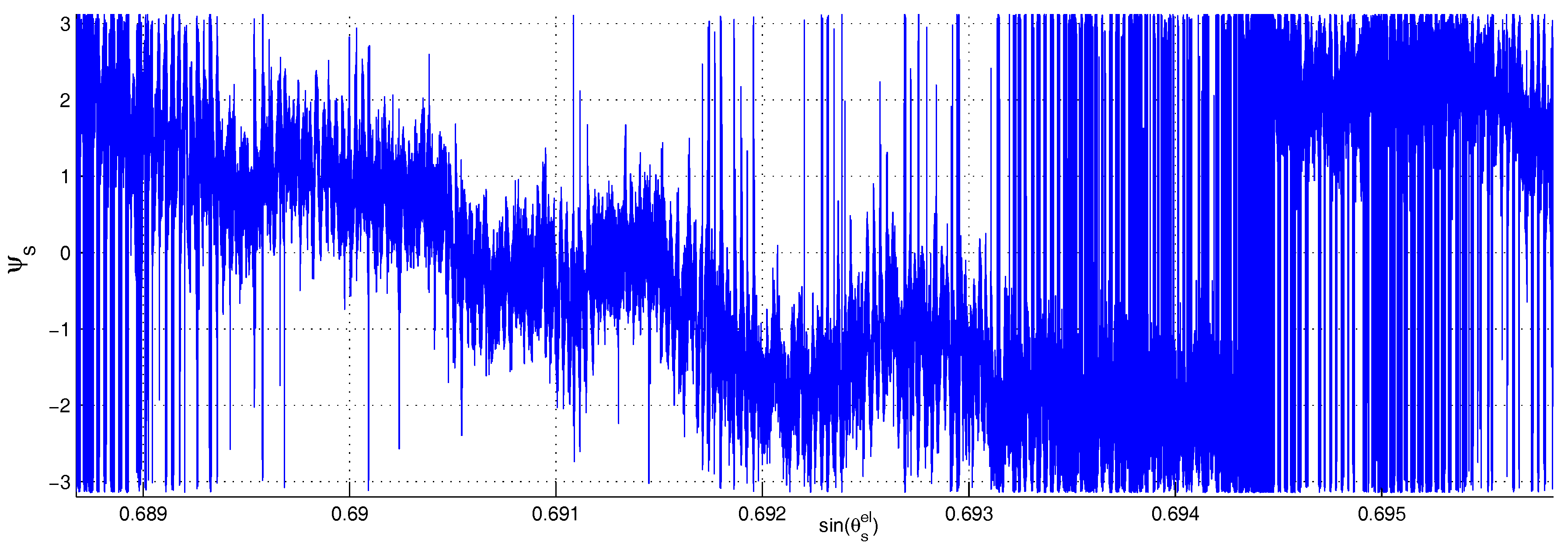
The first experiment took place on 30 June 2016. The reference height between the antennas and the water surface was 12.60 m. This height did not change during the experimentations, as the basin gates were locked. In Figure 9, an example of interferometric phase evolution in the time frame of the sine of the satellite elevation is shown. Each measure is obtained with one millisecond of coherent integration. In this figure, we observe, in accordance with Relation (4), that the phase difference evolves linearly as a function of the elevation sine. However, the linear slope is affected by oscillations that are not considered in our model. This effect can be due to the oscillations of the different elements of the system such as the mast or the surface of reflection.
The GPS satellites in view and their associated footprints on the basin are displayed in Figure 10. Only two footprints, corresponding to satellites PRN (Pseudo-Random Number) 18 and 21, can be used, as the footprint for satellite PRN 20 was partially out of sight during the experimentations. We acquired three successive sets of data at 15 h 25 min, 15 h 38 min and 15 h 51 min. For each dataset, the recording duration was of 600 s. We report in Table 2 the elevation and the carrier-to-noise ratio of the interferometric signal for each satellite.
Table 3 shows the estimated heights obtained for Satellites 18 and 21. On the first two lines of this table, the heights estimated independently for Satellites 18 and 21 at 15 h 25 min, 15 h 38 min and 15 h 51 min are presented. The estimated heights are within 10 cm of accuracy except for Satellite 21 at 15 h 51 min, with a difference with the tape measurement of 25 cm, and for Satellite 18 at 15 h 38 min and 15 h 51 min with a difference of 27 and 42 cm. For Satellite 21 at 15 h 51 min, the higher inaccuracy can be explained by the low of the signal. For Satellite 18 at 15 h 38 min and 15 h 51 min, the higher inaccuracy is explained by the low elevation rates (in absolute value), in accordance with the theoretical study. For observation durations of 600 s, the accuracy was expected to be of at least 5 cm according to this study. However, the additional oscillations, due to the waves being not taken into account in the model, affect the estimation precision. Over 600 s, the oscillations are averaged in the estimation process with some residuals. The loss of accuracy in the estimated height as compared to the theoretical study is supposed to be due to these residuals.
In order to improve the accuracy of the estimated height, we used the fusion operation defined in Equation (25) on the interferometric phase delays obtained for the two satellites. We present on the third line of Table 3 the estimated heights obtained at 15 h 25 min, 15 h 38 min and 15 h 51 min using this technique. The advantage is both to increase the amount of data and to increase the elevation sine span. At 15 h 25 min and 15 h 38 min, the estimated heights are both 1 cm close to the reference height. At 15 h 51 min, the estimated height is 9 cm away from the reference height. This can be explained looking at Figure 11, which shows the observed interferometric phases for Satellites 18 and 21 at 15 h 38 min and 15 h 51 min. In this figure, we observe that the elevation sine span is over two-times smaller at 15 h 51 min than at 15 h 38 min, explaining (through Equation (28)) the accuracy loss.
We present in Table 4 the estimated heights obtained with the fusion of the observations for Satellites 18 and 21 at 15 h 25 min, 15 h 38 min and 15 h 51 min, as a function of the considered observation duration. We show that for various elevation spans (of the order of 20 at 15 h 25 min, 10 at 15 h 38 min and a few degrees at 15 h 51 min), centimeter accuracy can be reached for any duration over 30 s (60,000 data points). This shows that fusing the data from several satellites can highly reduce the observation duration required for reaching a given accuracy. The main explanation is the increase of the elevation sine span. For a 15-s duration, the amount of data is not sufficient. This is in accordance with Figure 4: the equivalent number of data points (30,000) corresponds to the fast increase of the height estimation error.
In addition to merging data obtained from several satellites, it is also possible to merge data corresponding to different observation instants using the proposed estimator. On the fourth line of Table 3, we display the estimated height corresponding to the fusion of all of the available datasets, for both satellites and all three dates. The result of 12.60 m corresponds to the tape measured height.
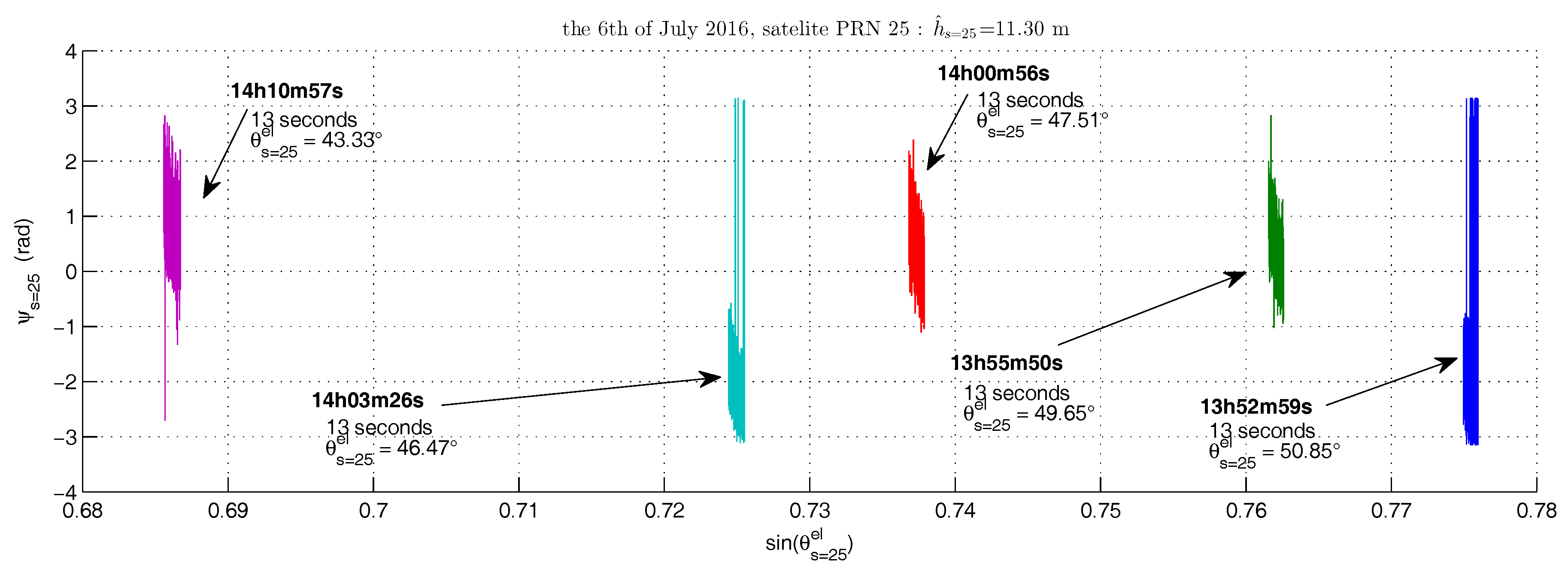
The second experiment took place on 6 July 2016 between 13 h 52 min and 14 h 10 min. The reference height between the antennas and the water surface was 11.27 m (constant height during the experimentation). The GPS satellites in view and the associated footprints are displayed Figure 12. The aim of this experiment is to show the feasibility of the proposed technique in the case of a single satellite signal observation including data losses. We considered the footprint of Satellite PRN 25 for this experimentation. We acquired five 13-s sets of data distributed over a 20-min span. Figure 13 shows the obtained interferometric phases as a function of the satellite elevation sine. We used all of the observations of phase for the height estimation, so the total amount of data corresponds to 65 s of observation (65,000 data points), with a satellite elevation varying over 20 min (in this case, over 7.5). The theoretical study thus predicts a good accuracy. The estimated height is 11.30 cm, three centimeters away from the tape measured height. This experimentation shows that the amount of data can be highly reduced if the span of variation of the satellite elevation is large. It also shows that the proposed linear-circular regression approach can be applied to sets with missing data, which could not be done in an estimation process including phase unwrapping. Such a case could correspond to signal losses or attenuations yielding to the selection of limited data intervals.
5. Discussion
The proposed receiver architecture and associated signal processing are applicable for static ground-based height measurements. In the dynamic case, the proposed method would only be valid for a constant height during the observation duration. The required observation duration for centimeter accuracy being linked with the number of observable reflected signals, very short durations could be sufficient with a multi-constellations and/or multi-frequency receiver. In the case of height variations during the measurements, the phase delay model and the associated regression estimator would have to be modified in order to be able to provide accurate, non-constant height estimation.
One of the drawbacks of the proposed technique is that the receiver altitude is limited. The largest observable path difference is indeed equal to 300 m (which corresponds to the C/A code length). The maximum observable height is 150 m for a satellite elevation of 90, 300 m for a satellite elevation of 30 and higher for lower elevations. Assuming the height is approximately known by other means (an accuracy of tens of meters is sufficient), this limitation can be avoided by adding the corresponding approximate code delay in the replicas (7) and (8). The other height limitation is linked to the assumption that the emitting satellite can be considered at an infinite distance from the observation zone: the technique described in this article is not applicable for spaceborne GNSS-R.
We found in the experimentation on real data the effects of the elevation variation span and observation duration that were predicted by the theoretical study. The main difference between the results on synthetic and real data is linked to the oscillations that affected the phase observations. These oscillations, which are not considered in the phase model, affected the data as an additional non-von Mises noise and altered the height estimation accuracy.
The classical approach used to improve the robustness of the estimation toward high noise levels is to reduce the filter bandwidth of the receiver. In the digital case, this is realized by increasing the correlation integration time, at the expense of time resolution. However, for high integration time, if the local replica frequency is not equal to the frequency of the received GNSS signal, the correlation to noise ratio is reduced. This problem can appear in the GNSS-R context if the direct and reflected signals have different frequencies. In addition, from a statistical point of view, using 1-ms integration time or more provides the same accuracy for the proposed estimator, as larger integration time provides less data points.
Larger integration times would be required for tracking the weak reflected signal in a classic lock loop. In the approach proposed in this article, the main advantage of the master/slave receiver architecture is that only the stronger direct signal has to be tracked. The interferometric GNSS-R (iGNSS-R) approach based on cross-correlating the direct and reflected received signals [22,41] allows using the military encrypted components of GNSS signals, leading to better performances than the proposed approach when only one satellite reflection is considered. However, iGNSS-R requires the use of directional antennas aiming at a single satellite signal. Being able to use omnidirectional antennas and to combine the data from several satellites reflections is a major advantage of the proposed method over iGNSS-R. Finally, in terms of signal processing, the linear-circular regression technique defined in this article can be used to get height estimates from datasets with large data gaps, which is something that cannot be done with the classical use of unwrapping techniques. Moreover, unwrapping can fail in the case of low , provoking cycle slips in the phase evolution and subsequently affecting the height estimation.
6. Conclusions
In this article, we present an innovative signal processing approach to ground-based GNSS-R phase altimetry. This approach is based on an original interferometry instrument providing phase delay observations that have a linear evolution in a certain time reference frame. The slope of this linear evolution provides a direct measurement of the height to estimate. In our approach, the phase observations are processed as angles, defined in the circular domain, and the measurement noise is assumed to follow a von Mises distribution. We accordingly derive a linear-circular regression estimator of the phase slope in the maximum likelihood sense. In an experimentation on synthetic data, we evaluate the proposed technique in terms of accuracy as a function of the satellite elevation span and of the signal carrier to noise ratio. We show that centimeter accuracy can be reached in common cases for a period of observation of 100 s. In an experimentation on real data, an original hardware receiver architecture is proposed. This architecture, based on the use of an optic fiber delay line, allows the separated recording of direct and reflected signals on a classic, inexpensive mono-channel receiver. The experiments on real data show that although GNSS-R signals are affected by external interferences that were not modeled, the centimeter accuracy can be obtained with the proposed estimator through various methods. When only one satellite footprint is available, a continuous observation of 10 min allows obtaining the decimeter accuracy. In that same context, a discontinuous observation of 1 min of data points over 20 min allows obtaining centimeter accuracy. This implies that the proposed altimetry technique can be used efficiently in the case of data losses. When several satellite footprints are available, two in the presented experimentations, the proposed estimator can fuse the available data and reach 1-cm accuracy for a 30-s continuous observation.
Acknowledgments
This work has been funded by the Pôle métropolitain Côte d’Opale de la région Hauts-de-France.
Author Contributions
Serge Reboul and Jean-Christophe Kucwaj proposed and derived the circular-linear regression and its application to GNSS-R phase altimetry. Jean-Christophe Kucwaj and Georges Stienne carried out the experiments on synthetic data. Jean-Christophe Kucwaj, Georges Stienne and Jean-Bernard Choquel designed and performed the experiments on real data. Jean-Christophe Kucwaj analyzed the data. All authors were involved in the writing of the paper.
Conflicts of Interest
The authors declare no conflict of interest.
References
- Martin-Neira, M. A passive reflectometry and interferometry system (PARIS): Application to ocean altimetry. ESA J. 1993, 17, 331–355. [Google Scholar]
- Garrison, J.; Komjathy, A.; Zavorotny, V.; Katzberg, S. Wind speed measurement using forward scattered GPS signals. IEEE Trans. Geosci. Remote Sens. 2002, 40, 50–65. [Google Scholar] [CrossRef]
- Masters, D.; Zavorotny, V.; Katzberg, S.; Emery, W. GPS signal scattering from land for moisture content determination. In Proceedings of the 2000 IEEE International Geoscience and Remote Sensing Symposium (IGARSS), Honolulu, HI, USA, 24–28 July 2000; Volume 7, pp. 3090–3092. [Google Scholar]
- Larson, K.M.; Gutmann, E.D.; Zavorotny, V.U.; Braun, J.J.; Williams, M.W.; Nievinski, F.G. Can we measure snow depth with GPS receivers? Geophys. Res. Lett. 2009, 36, L17502. [Google Scholar] [CrossRef]
- Rodriguez-Alvarez, N.; Bosch-Lluis, X.; Camps, A.; Ramos-Perez, I.; Valencia, E.; Park, H.; Vall-Llossera, M. Water level monitoring using the interference pattern GNSS-R technique. In Proceedings of the 2011 IEEE International Geoscience and Remote Sensing Symposium (IGARSS), Vancouver, BC, Canada, 24–29 July 2011; pp. 2334–2337. [Google Scholar]
- Larson, K.M.; Löfgren, J.S.; Haas, R. Coastal sea level measurements using a single geodetic GPS receiver. Adv. Space Res. 2013, 51, 1301–1310. [Google Scholar] [CrossRef]
- Ribot, M.A.; Kucwaj, J.C.; Botteron, C.; Reboul, S.; Stienne, G.; Leclère, J.; Choquel, J.B.; Farine, P.A.; Benjelloun, M. Normalized GNSS interference pattern technique for altimetry. Sensors 2014, 14, 10234–10257. [Google Scholar] [CrossRef] [PubMed]
- Alonso-Arroyo, A.; Camps, A.; Park, H.; Pascual, D.; Onrubia, R.; Martin, F. Retrieval of Significant Wave Height and Mean Sea Surface Level Using the GNSS-R Interference Pattern Technique: Results From a Three-Month Field Campaign. IEEE Trans. Geosci. Remote Sens. 2015, 53, 3198–3209. [Google Scholar] [CrossRef]
- Martin-Neira, M.; Caparrini, M.; Font-Rossello, J.; Lannelongue, S.; Vallmitjana, C.S. The PARIS concept: An experimental demonstration of sea surface altimetry using GPS reflected signals. IEEE Trans. Geosci. Remote Sens. 2001, 39, 142–150. [Google Scholar] [CrossRef]
- Treuhaft, R.N.; Lowe, S.T.; Zuffada, C.; Chao, Y. 2-cm GPS altimetry over Crater Lake. Geophys. Res. Lett 2001, 28, 4343–4346. [Google Scholar] [CrossRef]
- Lowe, S.T.; Zuffada, C.; Chao, Y.; Kroger, P.; Young, L.E.; LaBrecque, J.L. 5-cm-Precision aircraft ocean altimetry using GPS reflections. Geophys. Res. Lett. 2002, 29. [Google Scholar] [CrossRef]
- Cardellach, E.; Fabra, F.; Nogués-Correig, O.; Oliveras, S.; Ribó, S.; Rius, A. GNSS-R ground-based and airborne campaigns for ocean, land, ice, and snow techniques: Application to the GOLD-RTR data sets. Radio Sci. 2011, 46, RS0C04. [Google Scholar] [CrossRef]
- Carreno-Luengo, H.; Camps, A.; Ramos-Perez, I.; Rius, A. Experimental evaluation of GNSS-reflectometry altimetric precision using the P (Y) and C/A signals. IEEE J. Sel. Top. Appl. Earth Obs. Remote Sens. 2014, 7, 1493–1500. [Google Scholar] [CrossRef]
- Kucwaj, J.C.; Stienne, G.; Reboul, S.; Choquel, J.B.; Benjelloun, M. Accurate Pseudorange Estimation by Means of Code and Phase Delay Integration: Application to GNSS-R Altimetry. IEEE J. Sel. Top. Appl. Earth Obs. Remote Sens. 2016, 9, 4854–4864. [Google Scholar] [CrossRef]
- Fabra, F.; Cardellach, E.; Rius, A.; Ribó, S.; Oliveras, S.; Nogués-Correig, O.; Rivas, M.B.; Semmling, M.; Addio, S.D. Phase altimetry with dual polarization GNSS-R over sea ice. IEEE Trans. Geosci. Remote Sens. 2012, 50, 2112–2121. [Google Scholar] [CrossRef]
- Hobiger, T.; Haas, R.; Lofgren, J. Software-Defined Radio Direct Correlation GNSS Reflectometry by Means of GLONASS. IEEE J. Sel. Top. Appl. Earth Obs. Remote Sens. 2016, 9, 4834–4842. [Google Scholar] [CrossRef]
- Wang, G. Millimeter-accuracy GPS landslide monitoring using Precise Point Positioning with Single Receiver Phase Ambiguity (PPP-SRPA) resolution: A case study in Puerto Rico. J. Geod. Sci. 2013, 3, 22–31. [Google Scholar] [CrossRef]
- Semmling, M.; Beyerle, G.; Stosius, R.; Dick, G.; Wickert, J.; Fabra, F.; Cardellach, E.; Ribó, S.; Rius, A.; Helm, A.; et al. Detection of Arctic Ocean tides using interferometric GNSS-R signals. Geophys. Res. Lett. 2011, 38, L04103. [Google Scholar] [CrossRef]
- Kucwaj, J.C.; Stienne, G.; Reboul, S.; Choquel, J.B.; Benjelloun, M. A model-based angle unwrapper: Application to the GNSS-R Interference Pattern Technique. In Proceedings of the 2016 19th International Conference on Information Fusion (FUSION), Heidelberg, Germany, 5–8 July 2016; pp. 2095–2100. [Google Scholar]
- Semmling, A.; Wickert, J.; Schön, S.; Stosius, R.; Markgraf, M.; Gerber, T.; Ge, M.; Beyerle, G. A Zeppelin experiment to study airborne altimetry using specular global navigation satellite system reflections. Radio Sci. 2013, 48, 427–440. [Google Scholar] [CrossRef]
- Kucwaj, J.C.; Stienne, G.; Reboul, S.; Choquel, J.B.; Benjelloun, M. High rate interference pattern technique applied to real time altimetry. In Proceedings of the 2016 IEEE International Geoscience and Remote Sensing Symposium (IGARSS), Beijing, China, 10–15 July 2016; pp. 5631–5634. [Google Scholar]
- Zavorotny, V.U.; Gleason, S.; Cardellach, E.; Camps, A. Tutorial on remote sensing using GNSS bistatic radar of opportunity. IEEE Geosci. Remote Sens. Mag. 2014, 2, 8–45. [Google Scholar] [CrossRef]
- Lestarquit, L.; Peyrezabes, M.; Darrozes, J.; Motte, E.; Roussel, N.; Wautelet, G.; Frappart, F.; Ramillien, G.; Biancale, R.; Zribi, M. Reflectometry with an open-source software GNSS Receiver: Use case with carrier phase altimetry. IEEE J. Sel. Top. Appl. Earth Obs. Remote Sens. 2016, 9, 4843–4853. [Google Scholar] [CrossRef]
- Semmling, A.M.; Leister, V.; Saynisch, J.; Zus, F.; Heise, S.; Wickert, J. A phase-altimetric simulator: Studying the sensitivity of Earth-reflected GNSS signals to ocean topography. IEEE Trans. Geosci. Remote Sens. 2016, 54, 6791–6802. [Google Scholar] [CrossRef]
- Borre, K.; Akos, D.M.; Bertelsen, N.; Rinder, P.; Jensen, S.H. A Software-Defined GPS and Galileo Receiver: A Single-Frequency Approach; Springer Science & Business Media: Boston, MA, USA, 2007. [Google Scholar]
- Kaplan, E.; Hegarty, C. Understanding GPS: Principles and Applications; Artech House: Norwood, MA, USA, 2005. [Google Scholar]
- Cai, J.; Grafarend, E.W.; Hu, C. The statistical property of the GNSS carrier phase observations and its effects on the hypothesis testing of the related estimators. In Proceedings of the 20th International Technical Meeting of the Satellite Division of The Institute of Navigation (ION GNSS 2007), Fort Worth, TX, USA, 25–28 September 2007; pp. 331–338. [Google Scholar]
- Ghosh, K.; Jammalamadaka, S.R.; Vasudaven, M. Change-point problems for the von Mises distribution. J. Appl. Stat. 1999, 26, 423–434. [Google Scholar] [CrossRef]
- Sengupta, A.; Kumar Laha, A. A Bayesian analysis of the change-point problem for directional data. J. Appl. Stat. 2008, 35, 693–700. [Google Scholar] [CrossRef]
- Jammalamadaka, S.R.; Sengupta, A. Topics in Circular Statistics; World Scientific: Singapore, 2001; Volume 5. [Google Scholar]
- Mardia, K.V.; Jupp, P.E. Directional Statistics; John Wiley & Sons: Chichester, UK, 2009; Volume 494. [Google Scholar]
- Fisher, N.I. Statistical Analysis of Circular Data; Cambridge University Press: Cambridge, UK, 1995. [Google Scholar]
- Nikolaidis, N.; Pitas, I. Nonlinear processing and analysis of angular signals. IEEE Trans. Signal Proc. 1998, 46, 3181–3194. [Google Scholar] [CrossRef]
- Stienne, G.; Reboul, S.; Azmani, M.; Choquel, J.B.; Benjelloun, M. A multi-temporal multi-sensor circular fusion filter. Inf. Fusion 2014, 18, 86–100. [Google Scholar] [CrossRef]
- Stienne, G.; Reboul, S.; Azmani, M.; Choquel, J.B.; Benjelloun, M. GNSS dataless signal tracking with a delay semi-open loop and a phase open loop. Signal Proc. 2013, 93, 1192–1209. [Google Scholar]
- Marković, I.; Ćesić, J.; Petrović, I. Von Mises Mixture PHD Filter. IEEE Signal Proc. Lett. 2015, 22, 2229–2233. [Google Scholar] [CrossRef]
- Kurz, G.; Gilitschenski, I.; Julier, S.; Hanebeck, U.D. Recursive Bingham filter for directional estimation involving 180 degree symmetry. J. Adv. Inf. Fusion 2014, 9, 90–105. [Google Scholar]
- Routtenberg, T.; Tabrikian, J. Bayesian parameter estimation using periodic cost functions. IEEE Trans. Signal Proc. 2012, 60, 1229–1240. [Google Scholar] [CrossRef]
- Kurz, G.; Gilitschenski, I.; Hanebeck, U.D. Recursive Bayesian Filtering in Circular State Spaces. arXiv, 2015; arXiv:1501.05151. [Google Scholar]
- Hussin, A.G. Hypothesis Testing of Parameters for Ordinary Linear Circular Regression. Pak. J. Stat. Oper. Res. 2006, 2, 185–188. [Google Scholar] [CrossRef]
- Rius, A.; Nogués-Correig, O.; Ribó, S.; Cardellach, E.; Oliveras, S.; Valencia, E.; Park, H.; Tarongí, J.M.; Camps, A.; van der Marel, H.; et al. Altimetry with GNSS-R interferometry: First proof of concept experiment. GPS Solut. 2012, 16, 231–241. [Google Scholar] [CrossRef]
Figure 1.
Geometry of a ground-based GNSS-Reflectometry (R) altimeter.

Figure 2.
Construction of the observable.

Figure 3.
as a function of .

Figure 4.
RMSE and theoretical standard deviation of the estimated height as a function of the integration time, for various values of .
Figure 4.
RMSE and theoretical standard deviation of the estimated height as a function of the integration time, for various values of .

Figure 5.
Standard deviation of the estimated height as a function of the satellite elevation rate and for various initial elevations.
Figure 5.
Standard deviation of the estimated height as a function of the satellite elevation rate and for various initial elevations.
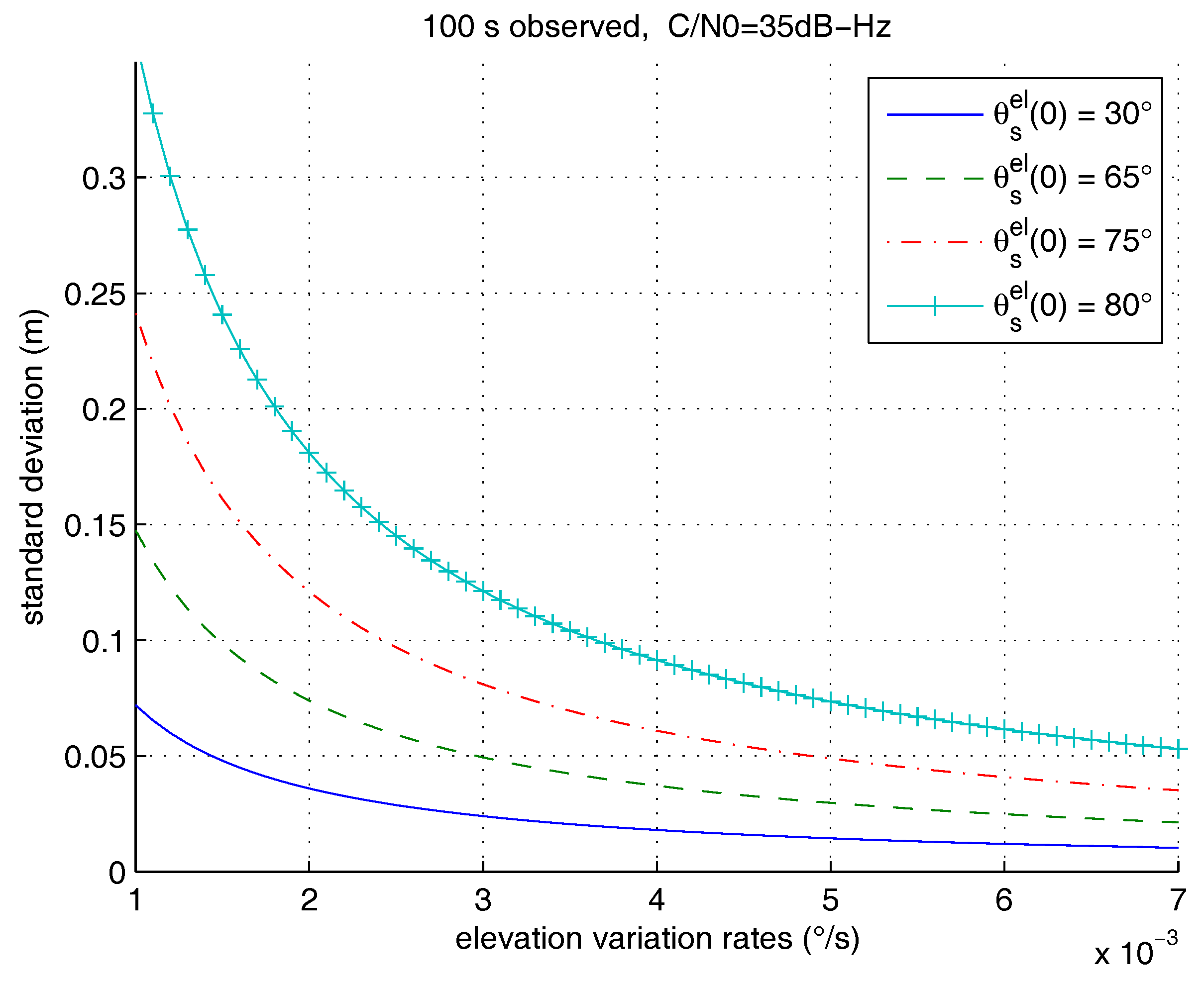
Figure 6.
Experimental setup.

Figure 7.
Example of delay-Doppler map obtained with the proposed receiver. The direct and reflected signals are separated in time by a delay = 5.12 s (in addition to the path delay).
Figure 7.
Example of delay-Doppler map obtained with the proposed receiver. The direct and reflected signals are separated in time by a delay = 5.12 s (in addition to the path delay).
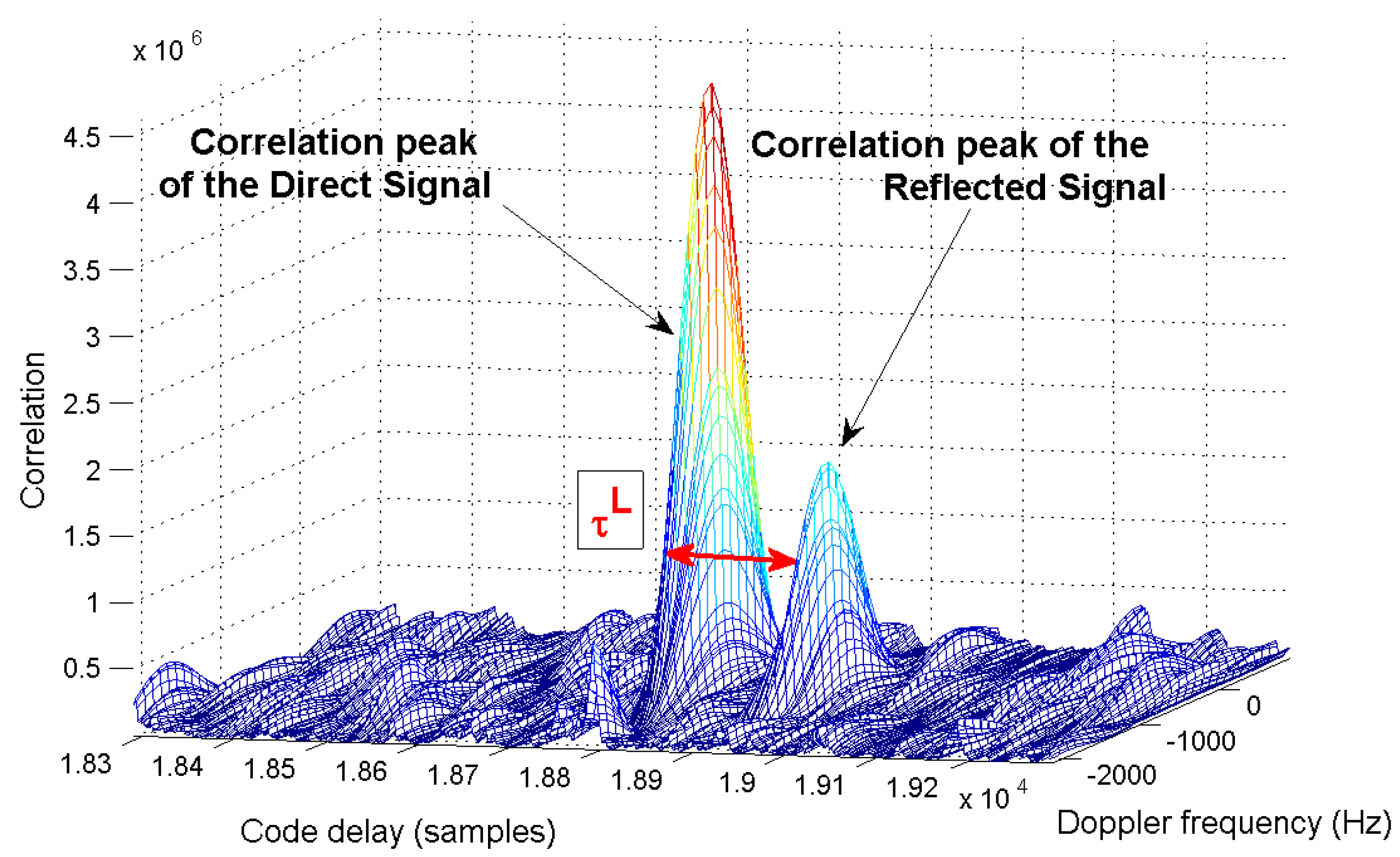
Figure 8.
Experimental vehicle carrying the GNSS-R altimeter. The observed GPS signals are reflected on an artificial basin in Calais, France (50.962689N, 1.857305E).
Figure 8.
Experimental vehicle carrying the GNSS-R altimeter. The observed GPS signals are reflected on an artificial basin in Calais, France (50.962689N, 1.857305E).

Figure 9.
Example of interferometric phase observations obtained for a GPS-L1 reflection on the artificial basin.
Figure 9.
Example of interferometric phase observations obtained for a GPS-L1 reflection on the artificial basin.

Figure 10.
GPS satellites in view and corresponding footprints on the basin 30 June 2016, 15 h 25 min.
Figure 10.
GPS satellites in view and corresponding footprints on the basin 30 June 2016, 15 h 25 min.
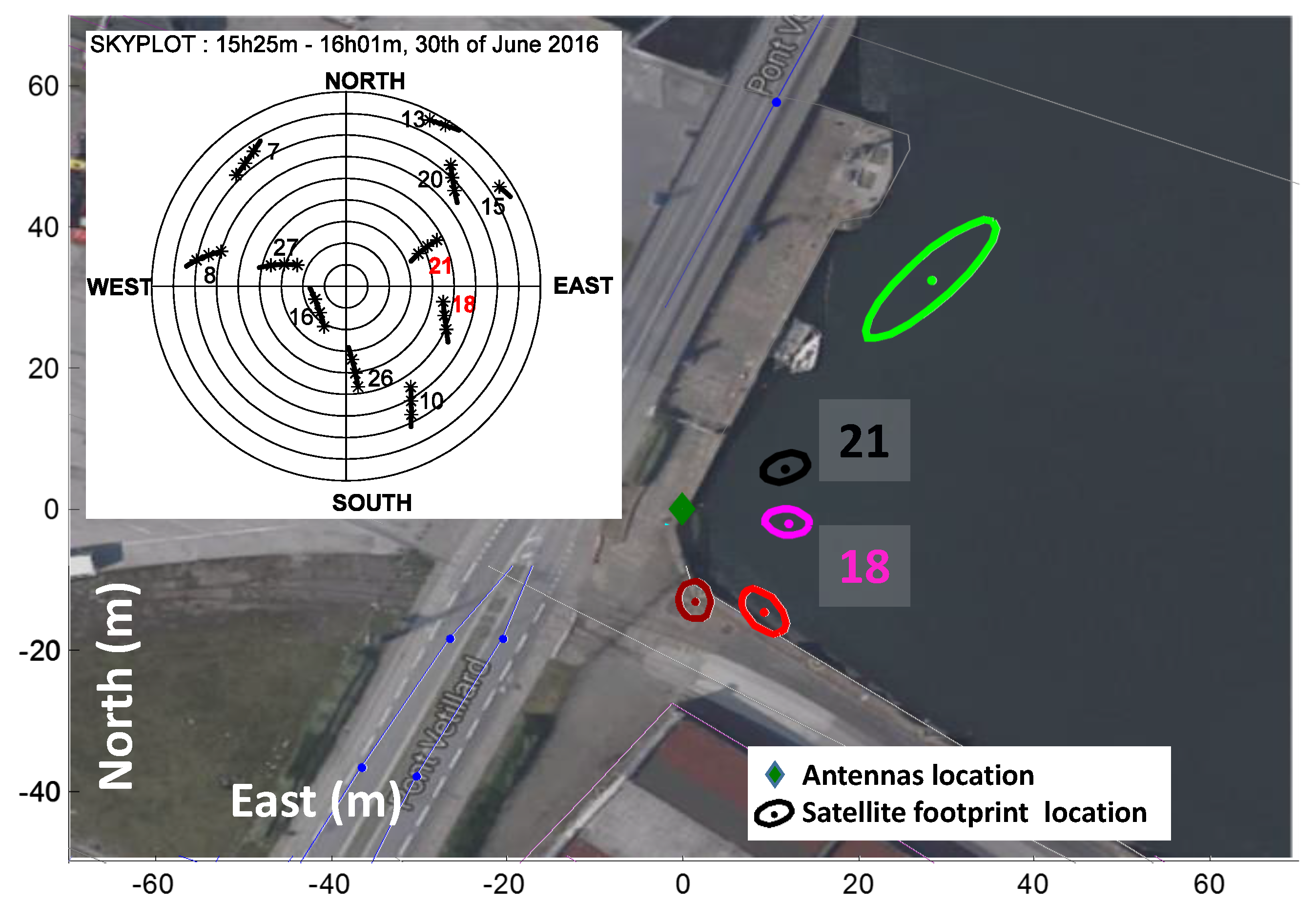
Figure 11.
(Left) Observed interferometric phase for Satellites 18 and 21 at 15 h 38 min, 30 June 2016. (Right) Observed interferometric phase for satellite 18 and 21 at 15 h 51 min, 30 June 2016.
Figure 11.
(Left) Observed interferometric phase for Satellites 18 and 21 at 15 h 38 min, 30 June 2016. (Right) Observed interferometric phase for satellite 18 and 21 at 15 h 51 min, 30 June 2016.
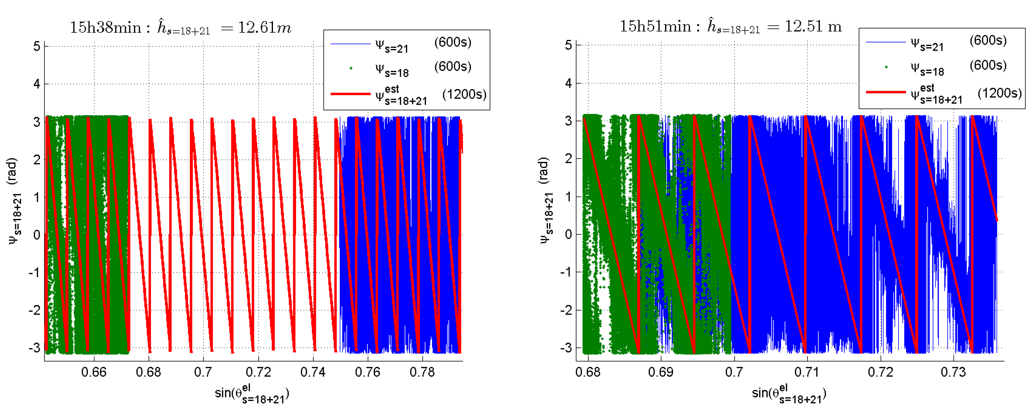
Figure 12.
GPS footprints on the canal basin, 6 July 2016 at 13 h 59 min.

Figure 13.
Observed interferometric phase from Satellite 25.

Table 1.
Concentration parameter corresponding to various values of the interferometric signal.
| (dB-Hz) | 30 | 35 | 40 | 45 |
| 1.35 | 2.96 | 9.34 | 30.82 |
Table 2.
Parameters for satellites PRN 18 and 21, 30 June 2016, during 600 s of observation at 15 h 25 min, 15 h 38 min and 15 h 51 min.
Table 2.
Parameters for satellites PRN 18 and 21, 30 June 2016, during 600 s of observation at 15 h 25 min, 15 h 38 min and 15 h 51 min.
| 15 h 25 min | |||||
| Satellite PRN | Interferometric Signal C/ (dB-Hz) | Elevation | |||
| min. () | max. () | mean () | rate (/s) | ||
| 18 | 36.5 | 36.44 | 39.21 | 37.85 | 0.0046 |
| 21 | 34 | 53.73 | 57.56 | 55.65 | −0.0064 |
| 15 h 38 min | |||||
| Satellite PRN | Interferometric Signal / (dB-Hz) | Elevation | |||
| min. () | max. () | mean () | rate (/s) | ||
| 18 | 37 | 39.99 | 42.23 | 41.15 | 0.0037 |
| 21 | 34.1 | 48.55 | 52.51 | 50.53 | −0.0066 |
| 15 h 51 min | |||||
| Satellite PRN | Interferometric Signal / (dB-Hz) | Elevation | |||
| min. () | max. () | mean () | rate (/s) | ||
| 18 | 35 | 42.80 | 44.38 | 43.63 | 0.0026 |
| 21 | 32.3 | 43.39 | 47.38 | 45.38 | −0.0066 |
Table 3.
Estimated heights 30 June 2016 for 600 seconds of observation, Satellites PRN 18 and 21.
| Satellite PRN | 15 h 25 min | 15 h 38 min | 15 h 51 min |
|---|---|---|---|
| m | m | m | |
| Estimated Height (m) | Estimated Height (m) | Estimated Height (m) | |
| 18 | 12.68 | 12.87 | 13.02 |
| 21 | 12.65 | 12.49 | 12.36 |
| 18 + 21 | 12.61 * | 12.61 * | 12.51 * |
| 18 + 21 | 12.60 ** | ||
* Results obtained using the proposed fusion operation on both satellites. ** Results obtained using the proposed fusion operation on both satellites and all recordings.
Table 4.
Estimated height (m) as a function of the observation duration, obtained by fusion of Satellite 18 and 21 data at 15 h 25 min, 15 h 38 min and 15 h 51 min, 30 June 2016 (reference height: m.)
Table 4.
Estimated height (m) as a function of the observation duration, obtained by fusion of Satellite 18 and 21 data at 15 h 25 min, 15 h 38 min and 15 h 51 min, 30 June 2016 (reference height: m.)
| Sat.: 18 + 21 | 15 s | 30 s | 50 s | 100 s | 150 s | 300 s | 600 s |
|---|---|---|---|---|---|---|---|
| 15 h 25 min | 8.80 | 12.63 | 12.62 | 12.62 | 12.61 | 12.62 | 12.61 |
| 15 h 38 min | 7.54 | 12.62 | 12.61 | 12.61 | 12.62 | 12.62 | 12.61 |
| 15 h 51 min | 16.01 | 12.56 | 12.53 | 12.54 | 12.55 | 12.55 | 12.51 |
© 2017 by the authors. Licensee MDPI, Basel, Switzerland. This article is an open access article distributed under the terms and conditions of the Creative Commons Attribution (CC BY) license (http://creativecommons.org/licenses/by/4.0/).
Share and Cite
MDPI and ACS Style
Kucwaj, J.-C.; Reboul, S.; Stienne, G.; Choquel, J.-B.; Benjelloun, M. Circular Regression Applied to GNSS-R Phase Altimetry. Remote Sens. 2017, 9, 651. https://doi.org/10.3390/rs9070651
AMA Style
Kucwaj J-C, Reboul S, Stienne G, Choquel J-B, Benjelloun M. Circular Regression Applied to GNSS-R Phase Altimetry. Remote Sensing. 2017; 9(7):651. https://doi.org/10.3390/rs9070651
Chicago/Turabian StyleKucwaj, Jean-Christophe, Serge Reboul, Georges Stienne, Jean-Bernard Choquel, and Mohammed Benjelloun. 2017. "Circular Regression Applied to GNSS-R Phase Altimetry" Remote Sensing 9, no. 7: 651. https://doi.org/10.3390/rs9070651
Note that from the first issue of 2016, this journal uses article numbers instead of page numbers. See further details here.