
Ground Truth of Passive Microwave Radiative Transfer on Vegetated Land Surfaces


1
Department of Civil Enginneering, the University of Tokyo, Tokyo 113-8656, Japan
2
Data Assimilation Research Team, RIKEN Advanced Institute for Computational Science, Kobe 650-0047, Japan
3
Meteorological Research Institute, Japan Meteorological Agency, Tsukuba 305-0052, Japan
4
Earth Observation Research Centor, Japan Aerospace Exploration Agency, Tsukuba 305-8505, Japan
5
International Centre for Water Hazard and Risk Management (ICHARM), Tsukuba 305-8516, Japan
*
Author to whom correspondence should be addressed.
Remote Sens. 2017, 9(7), 655; https://doi.org/10.3390/rs9070655
Submission received: 15 May 2017
/
Revised: 12 June 2017
/
Accepted: 21 June 2017
/
Published: 26 June 2017
(This article belongs to the Section Remote Sensing in Geology, Geomorphology and Hydrology)
Abstract
:In this paper, we implemented the in-situ observation of surface soil moisture (SSM), vegetation water content (VWC), and microwave brightness temperatures. By analyzing this in-situ observation dataset and the numerical simulation, we investigated the source of the uncertainty of the current algorithms for Advanced Microwave Scanning Radiometer for Earth observation system (AMSR-E) and AMSR2 to retrieve SSM and vegetation dynamics. Our findings are: (1) the microwave radiative transfer at C-band and X-band is not strongly affected by the shape of vegetation and the existing algorithm can be applied to a wide variety of plant types; (2) the diversity of surface soil roughness significantly affects the indices which are used by the current algorithms and addressing the uncertainty of surface soil roughness is necessary to improve the retrieval algorithms; (3) At C-band, SSM of the homogeneous vegetated land surfaces can be detected only when their VWC is less than approximately 0.25 (kg/m2); (4) the state-of-the-art Radiative Transfer Model (RTM) can predict our observed dataset although we have some biases in simulating brightness temperatures at a higher frequency. The new in-situ observation dataset produced by this study can be the guideline for both developers and users of passive microwave land observations to consider the uncertainties of their products.
1. Introduction
Passive microwave satellite observations have been used extensively to monitor global surface soil moisture (SSM) and vegetation dynamics, and contributed to deepen the understandings of hydrological and biogeochemical cycles. For example, Anderson et al. [1] developed the drought monitor in East Africa using the soil moisture product from Advanced Microwave Scanning Radiometer for Earth observation system (AMSR-E). Taylor et al. [2] investigated soil moisture-precipitation feedback globally using soil moisture data from AMSR-E. Liu et al. [3] developed the long-term global aboveground biomass carbon dataset from vegetation optical depth (VOD), which is correlated to vegetation water content (VWC), from Special Sensor Microwave Imager (SSM/I), AMSR-E, FengYun-3B Microwave Radiometer Imager (MWRI) and Windsat. Zhou et al. [4] detected the widespread decline of Congo rainforest by analyzing VOD data from AMSR-E. In addition, datasets of passive microwave satellite observations have been assimilated to land surface models in order to improve their performance of simulating water and energy fluxes (e.g., [5,6,7,8,9,10,11]).
Most of the currently available algorithms solve an inversion of a radiative transfer model (RTM) to retrieve SSM and VOD (or VWC) from passive microwave brightness temperatures [12,13,14,15]. Their RTMs include a calculation of the dielectric constant of soil-water mixture (e.g., [16]), soil emissivity which includes the effect of soil surface scattering (e.g., [17]), and radiative transfer in a vegetation canopy (e.g, [18]). To improve the efficiency of numerically solving the inversion of RTM, previous studies have used some useful indices calculated by multi-polarized and multi-frequency brightness temperatures, such as Polarization Index (PI) [19] and Index of Soil Wetness (ISW) [14]. They have also used some validated empirical relationships such as the linear relationship between surface physical temperature and brightness temperature of 37 GHz [12,20].
However, these RTM inversions are ill-posed problems. In addition to SSM and VOD (or VWC), vegetation structure information (e.g., single scattering albedos), surface soil roughness, and soil texture information are often necessary to run RTM. Although these valuables have great diversity on Earth surface, it is impossible to determine every parameter of RTM from brightness temperatures which are observed by currently available satellites. Therefore, many algorithms assumed fixed conditions of single scattering albedos and surface soil roughness [12,14,15] although some efforts have been made to objectively estimate these parameters by introducing other satellite observations (i.e., visible/infrared satellite observations) (e.g., [21,22]). This assumption brings significant uncertainties of their retrievals [23,24]. In addition, since penetration depths of C-band and L-band microwaves are limited, the observed brightness temperatures lose their sensitivity to SSM and VWC as vegetation density increases, which also brings large uncertainty of the retrievals on vegetated surfaces (e.g., [25,26,27]).
It is extremely difficult to quantitatively evaluate these uncertainties at the satellite footprint scales due to variability of soil and vegetation within coarse footprint pixels. Although numerous studies have contributed to collect ground observations of passive microwave brightness temperatures and land surface information using ground-based radiometers (e.g., [28]), there are the limited number of in-situ SSM, VWC, and passive microwave brightness temperatures’ observations that are continuous over a long period of time, cover a wide variety of vegetation types under a consistent experiment design to evaluate the effect of variation of vegetation structure and surface soil roughness.
The aim of this study is to provide and analyze the dataset of in-situ observations of SSM, VWC, and brightness temperatures for a wide variety of plants, from short crops to tall trees. Here we focus on brightness temperatures with frequencies which are available to AMSR-E and AMSR2. By performing and analyzing these in-situ observations, we would like to answer the following questions: (1) how strongly does the shape of vegetation influence microwave radiative transfer? (2) what is the major source of the uncertainties in SSM and VWC retrieval? (3) how sensitive are microwave brightness temperatures to SSM with moderate and dense vegetation covers? (4) Is the state-of-the-art RTM consistent to the in-situ ground truth regarding to the uncertainties of SSM and VWC retrievals? Our ground truth can be the guideline for both developers and users of passive microwave land observations to consider the uncertainties of their products.
The remainder of this paper is organized as follows. In Section 2, we briefly review some existing SSM and VOD (or VWC) retrieval algorithms and specify the important relationships to be validated by in-situ observations. In Section 3, we describe the design of our field measurements and RTM simulations. The results are provided in Section 4 and we describe conclusions in Section 5.
2. Theoretical Background
Here we briefly review the important processes of microwave radiative transfer which should be validated by our ground truth data.
2.1. Surface Physical Temperature Retrieval
Since the primary factor which controls microwave brightness temperatures is physical temperature, the effect of the variation of physical temperature should be minimized to quantify the effect of SSM and VOD on the emissivity. To retrieve surface physical temperature from microwave observations, the empirical linear relationship between physical temperatures and 37 GHz vertical polarized brightness temperatures is often used. For example, the Land Parameter Retrieval Model (LPRM; [12,29]) uses the following empirical equation:
where Ts is the surface physical temperature (K) and TB,37V is the 37 GHz vertical polarized brightness temperature (K). The 37 GHz vertical polarized brightness temperature balances a reduced sensitivity to soil surface characteristics with a relatively high atmosphere transmissivity [20], which make it suitable to the physical temperature retrieval. The Equation (1) was thoroughly validated using the network of meteorological towers [20].
It should be noted that the Equation (1) cannot be applied in freezing conditions and the accuracy is reduced in barren, sparsely vegetated and open shrublands [20]. In addition, Holmes et al. [20] has confirmed that this linear relationship is highly affected by the assumption of the values of single scattering albedos.
2.2. Vegetation Retrieval
Polarization Index (PI; [19]) has been widely accepted as an index which is sensitive to VWC [12,14,15]. PI is the normalized polarization difference of brightness temperatures and can be defined as:
where TB,V and TB,H are vertical and horizontal polarized brightness temperature, respectively. Because the difference between vertical polarized and horizontal polarized brightness temperatures is reduced by the extinction process within the vegetation layer, PI decreases as VWC increases. One of the advantages of PI is that the effect of physical temperatures on PI is minimal.
Although the relationship between PI and VWC has been validated in the previous studies (e.g., [19,30]), it is highly affected by land surface conditions (i.e., SSM and surface soil roughness) [22] and single scattering albedos [31]. It is important to evaluate the robustness of the PI-VWC relationship with a wide variety of land surface conditions and vegetation types.
2.3. Surface Soil Moisture Retrieval
One of the methods to retrieve SSM is to directly compare the RTM-estimated and satellite-observed surface emissivities. In the LPRM, the emissivity can be calculated since the physical temperature has been obtained using the empirical relationship described in Section 2.1. Then, if the correct VOD has already been obtained, the dielectric constant of soil, which is the function of SSM, can be calculated by inversely solving the soil surface RTM. Since an observed emissivity is highly affected by vegetation, retrieved SSM would be biased if the accurate VOD has not been obtained. Therefore, the simultaneous retrieval of SSM and VOD, is necessary. It should be mentioned that surface soil roughness also significantly affects a soil surface emissivity although LPRM does not consider the variety of surface soil roughness. The other limitation of this approach is that biases of the physical temperature retrieval described in Section 2.1 greatly affect their SSM retrieval.
The other method to retrieve SSM from microwave observations is to utilize the difference of brightness temperatures in different frequencies. For example, the Japan Aerospace eXploration Agency (JAXA) standard algorithm (hereafter JAXA; [14,15]) uses Index of Soil Wetness (ISW) as an index sensitive to SSM [14]. ISW is defined as a following equation:
where TBi and TBj are the brightness temperatures of high and low frequencies, respectively. Since the dielectric constant of water is dependent to a frequency, the change of emissivity due to soil moisture’s change strongly depends on the frequency. Therefore, ISW is sensitive to SSM. The advantage of ISW is that the effect of physical temperature changes on ISW is minimal.
However, ISW is also highly sensitive to VOD (or VWC) so that the simultaneous retrieval of SSM and VOD is necessary. In addition, the effect of surface soil roughness cannot be eliminated by introducing ISW although the JAXA algorithm assumes the fixed value of the surface soil roughness parameters of their RTM [15].
3. Methods and Materials
3.1. In-Situ Observation
We implemented the field measurement at Tanashi observation site, which is in the Institute for Sustainable Agro-ecosystem Services, Graduate School of Agricultural and Life Sciences, the University of Tokyo. The site is located in the western part of the Tokyo metropolitan area, Japan.
We installed a ground-based microwave radiometer (GBMR) in the field (Figure 1). This GBMR has four channels which cover the frequency ranges of 6.925, 10.65, 36.5, and 89 GHz at both horizontal and vertical polarizations. The detailed information about this GBMR (e.g., the height of the sensors, the sizes of footprint, and the sidelobe levels) can be found in [22]. The incident angle was set to 55 degrees, which is same as for AMSR-E and AMSR2. We obtained brightness temperatures by taking the average over 100 samples.
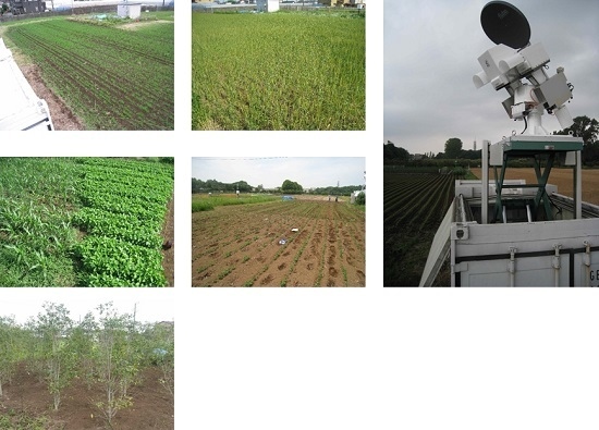
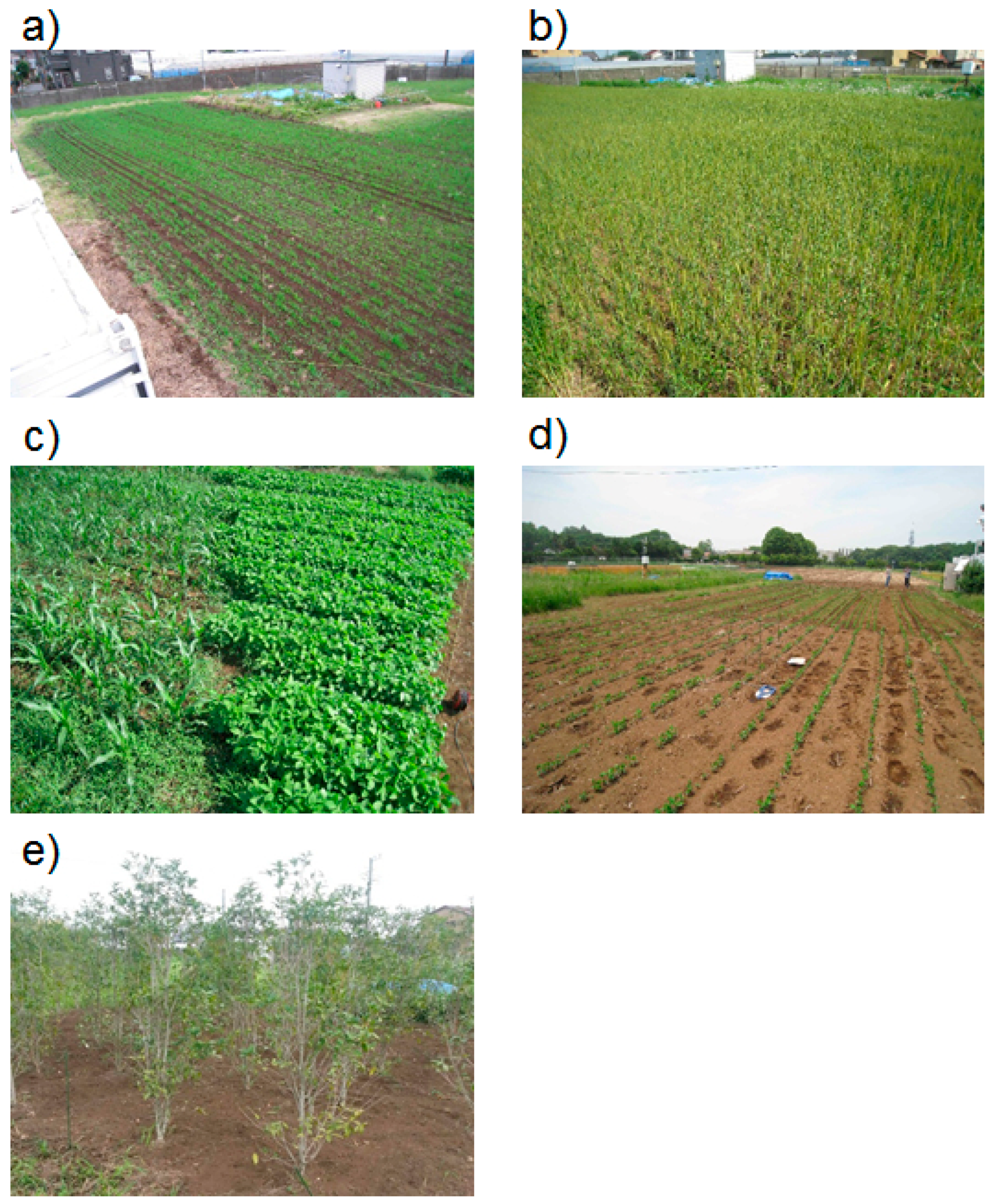
Table 1 summarizes our observation schedules and Figure 2 provides the condition of the footprints in each observation period. We planted oat, wheat, soybean, corn, and olive. Observations of period I–III have already been used by [22] to develop the SSM and VWC retrieval algorithm. In this paper, we analyzed observations of period IV and V as well as those of period I–III to derive the ground truth of microwave radiative transfer on vegetated surfaces. All in-situ observation data which we used in this paper can be downloaded as a supplemental material of this paper (Supplement Data S1).
We planted vegetation at the site and sampled them to measure their leaf area, dry mass and VWC. In Phase I–IV, we did not perform sampling at the GBMR’s footprint and we used the sampling area where we planted vegetation with the same density as the GBMR’s footprint. On the other hand, in some of the observations in Phase V, we directly sampled the olive trees from the GBMR’s footprint. This is because the olive trees do not change their mass during our short-term observation and we need to artificially change their VWC and dry mass by clipping and removing parts of the plant. Specifically, for one footprint, we removed all leaves of trees in the footprint and implemented the observation. Then we removed all brunches of trees in the footprint and collected the observation. Finally we removed every aboveground biomass to calculate their total mass. For the other footprint, we halved their height and implemented the observation. Then we removed every aboveground biomass and calculated their total mass. VWC was calculated as the difference between the mass of wet and dry biomass.
We observed SSM using a time-domain reflectometer. The measured SSM represents approximately 0–5 cm depth soil moisture. The surface physical temperatures were also observed by the infrared thermometers.
3.2. Radiative Transfer Model
An RTM was used in this paper for two reasons. First, we evaluated if our RTM can reproduce the results of our in-situ observation. Second, we interpreted our observations by analyzing the results of our RTM simulation.
The RTM has been developed and used by [8,9,17,22]. In this RTM, surface reflectivity is calculated by the advanced integral equation model (AIEM) [32] with an incorporated shadowing effect [17]. The equation to get soil surface reflectivity is the following:
where p and q refer to the polarization state (vertical (V) and horizontal (H)), Rp is the reflectivity of the land surface, rp is the Fresnel reflectivity, k is the wave number, σ is the RMS height, hpp and hpq are the single scattering terms, j is the scattering direction, and θ is the incidence angle, and φ is the azimuth angle. S is the shadowing function, which is dependent on the surface roughness parameters (RMS height and correlation length). Complete equations can be found in [17]. In this model, the dielectric constant of the soil-water mixture is calculated using the method developed by [33].
We used the tau-omega model [18] to obtain the total emission and attenuation from the land surface and vegetation canopy using the following equation:
where TBp is the brightness temperature at the radiometer level, Ts is the physical land surface temperature, Tc is the canopy temperature, is the single scattering albedo of the canopy, and subscript p indicates polarizations (vertical (V) or horizontal (H)). VOD is the vegetation optical depth, which has the linear relationship with VWC. In this study, we assume , which is widely accepted in the previous studies (e.g., [15,19,22]).
VOD is linearly correlated with VWC [28] as the following equation:
where VWC is vegetation water content, is the wavelength of microwave, and are parameters.
To investigate the behavior of the RTM and compare it with the in-situ observations, we calculated the brightness temperatures of 6.925 GHz, 10.35 GHz, and 36.5 GHz with many combinations of RTM inputs which are SSM, VWC, vertical and horizontal single scattering albedos, and RMS height. The datasets of the combinations of brightness temperatures and RTM inputs are called the LookUp Tables (LUTs) in the previous studies [15]. Table 2 shows the range of the RTM inputs of the LUT generated in this study. The LUT has 1,000,000 combinations of brightness temperatures and RTM inputs (100 SSM bins × 100 VWC bins × 10 vertical single scattering albedo bins × 10 horizontal single scattering albedo bins × 10 RMS height bins). Table 2 also shows the values of some fixed parameters of the RTM when we generated the LUT. Since we obtained no prior information of single scattering albedos and surface soil roughness in this study, the ranges of these values in the LUT were chosen based on the selected values by the previous studies [12,13,14,15]. We will compare the structure of this LUT and the in-situ observations.
We implemented the simple sensitivity analysis for the RTM by analyzing the LUT. For example, when we define our target valuable (e.g., PI or ISW) , the sensitivity of SSM to this objective value with given other inputs, was calculated by:
where i, j, k, l and m are bin numbers for SSM, VWC, vertical single scattering albedo, horizontal single scattering albedo, and RMS height, respectively. is the increment for the change of the RTM input to evaluate the sensitivities and the values of are summarized in Table 2.
4. Results
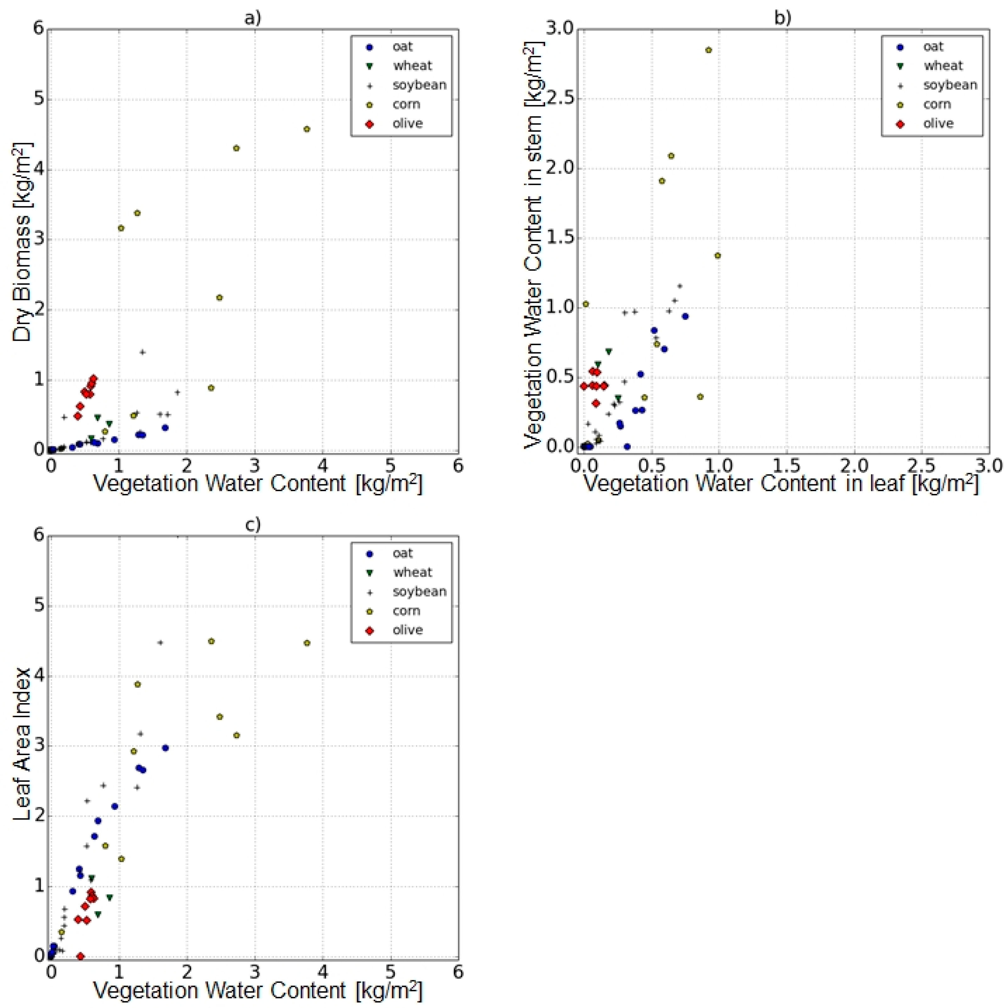
Our primary target is to evaluate how the microwave radiative transfer is sensitive to the vegetation types. Figure 3a–c show that the observed plants have diverse structures. Figure 3a shows that the dry mass and VWC for oat, wheat, soybean, corn, and olive tree. Dry carbon biomass of olive trees is heavier than VWC while dry carbon biomass of other crops (oat, wheat, and soybeans) are often lighter than VWC. Plots of corns are scattered mainly due to sampling errors and decrease in VWC with unchanged dry mass as they were dying. Figure 3b shows that the olive trees and wheat have a larger amount of VWC in stems than oat, soybeans, and corns. Although oat and wheat generally have similar morphology, they have different ratio of VWC in stem to that in leaf probably because they were planted and raised in the different seasons (see Table 1) and they showed different phenology. Figure 3c also shows that the olive trees and wheat have smaller LAI than other crops.
In Section 4.1, we evaluate the in-situ observed relationship between 37 GHz vertically polarized brightness temperatures and ground physical temperatures. In Section 4.2, we evaluate the robustness of the relationship between PI and VWC at 6.925 GHz and 10.65 GHz. In Section 4.3, we analyze the in-situ observed relationship between emissivities and SSM and the relationship between ISW and SSM. We discuss the possibility to observe SSM under the vegetation canopy.
4.1. 37 GHz Vertical Brightness Temperature—Physical Temperature Relationship
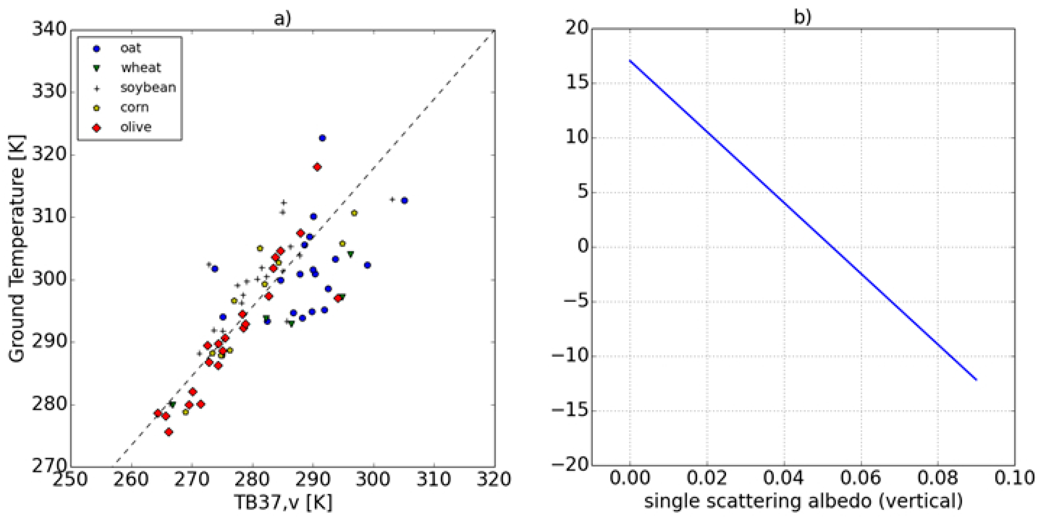
Figure 4a shows the relationship between 36.5 GHz vertical-polarized brightness temperatures and ground physical temperatures for oat, wheat, soybeans, corns, and olive trees. The dashed line indicates the empirical model of [20] (Equation (1)). The empirical relationship of [20] has a good performance to predict our in-situ observed ground temperature data.
According to [20], the largest source of errors in this relationship is the uncertainty of single scattering albedo. Following the analysis by [20], we calculate the bias of Equation (1) using calculated 36.5 GHz vertical polarized brightness temperatures with various single scattering albedos in the LUT. The LUT has the fixed surface physical temperature (293 (K)). This physical temperature is “truth” in the LUT. The LUT also has 36.5 GHz vertical-polarized brightness temperatures by driving the RTM so that we can calculate the surface physical temperature from this brightness temperature using Equation (1). This is the “estimated” physical temperature by Equation (1). Figure 4b shows the difference between “truth” and “estimated” physical temperatures as a function of single scattering albedo. Figure 4b indicates that the Equation (1) is unbiased with the assumption that single scattering albedo is approximately 0.05, which is consistent to [20]. However, the Equation (1) may have large errors with the plants which have smaller or larger single scattering albedo than 0.05. Figure 4a shows that the performance of the Equation (1) is degraded for the footprint of oat, which might be due to the small single scattering albedos of oat.
4.2. PI-VWC Relationship
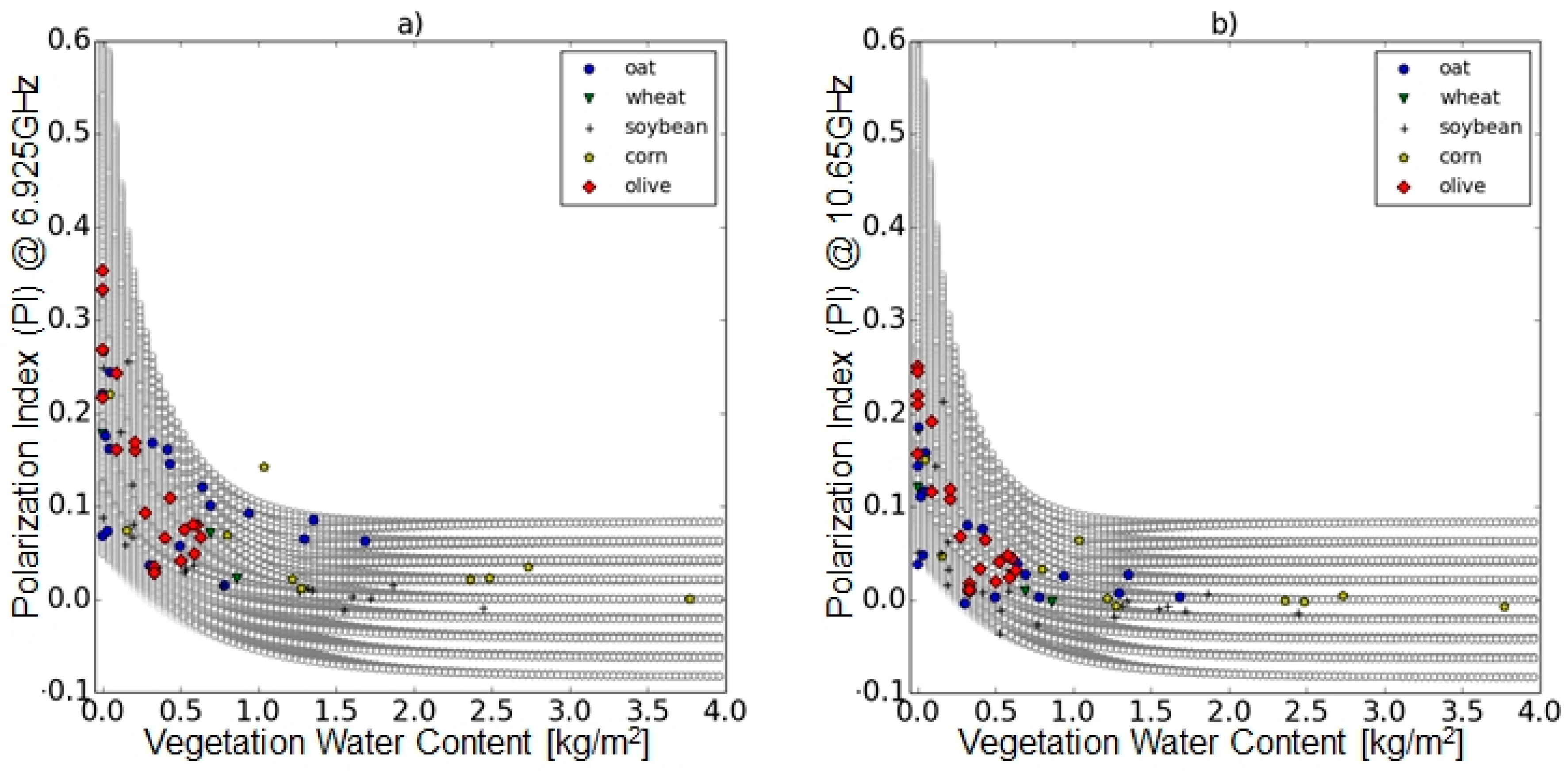
Figure 5a,b show the relationship between PI and VWC at 6.925 GHz and 10.65 GHz, respectively. First, although PI monotonically decreases as VWC increases, the sensitivity of VWC to PI at 6.925 GHz and 10.65 GHz is small if VWC is larger than 1.5 (kg/m2) and 1.0 (kg/m2), respectively. Second, the variances of PI under same VWC increase as VWC decrease. Third, the PI-VWC relationship is independent to the plant’s type.
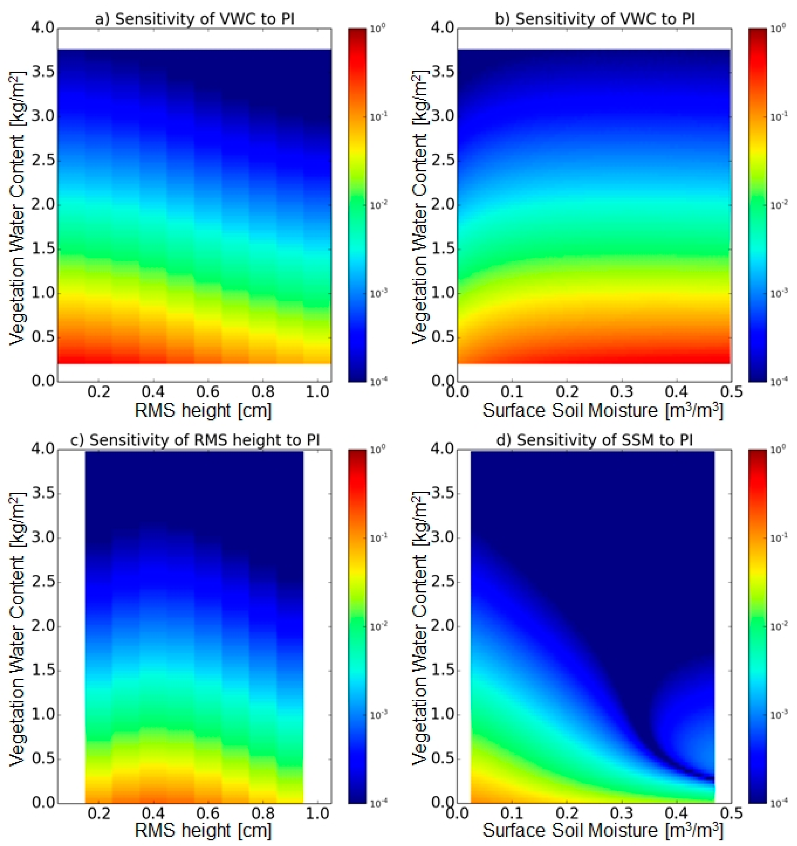
These findings are consistent to the LUT sensitivity analysis. Figure 6a,b show the sensitivity of VWC to PI at 6.925 GHz as a function of soil surface roughness and SSM, respectively. The sensitivity of VWC to PI rapidly decreases as VWC increases. When VWC is 1.5 (kg/m2), the change of PI generated by the 0.4 (kg/m2) change of VWC is the order of 0.01, which is cannot be detected in the real world applications. Figure 6a also indicates that PI is more sensitive to VWC on smooth surfaces than rough surfaces. On the other hand, the sensitivity of VWC to PI is not significantly affected by soil wetness (Figure 6b).
The large variances of PI under small VWC mainly come from the variability of surface soil roughness. Figure 6c shows the change in PI generated by the 2.0 (mm) change in RMS height. When VWC is less than 0.5 (kg/m2), the sensitivity of RMS height to PI is the order of 0.1. Considering that we generally do not have any a priori information on surface soil roughness, this sensitivity of RMS height to PI is significantly large. In our in-situ observation, we randomly cultivate the field before seeding and surface soil roughness may change during the one observation period due to wind, precipitation, and our land management (e.g., removing weeds). Therefore, we can conclude that the most important uncertainty of the observed PI-VWC relationship is the uncertainty of surface soil roughness.
The sensitivity of SSM to PI is relatively small although it cannot be neglected. Figure 6d shows the change in PI generated by the 0.05 (m3/m3) change in SSM. Although an increment of SSM for the sensitivity analysis is large (=0.05 (m3/m3)), the sensitivity of SSM to PI is smaller than VWC and RMS height.
The bifurcation of gray lines with high VWC (>1.5 (kg/m2)) is induced by the polarization differences of single scattering albedos. The polarization difference of single scattering albedos is important in the case of high VWC [31]. However, compared with the effect of uncertainty of RMS height, the sensitivity of single scattering albedos to PI is smaller. The 0.02 change in single scattering albedos induces the change in PI with the order of 0.01 (not shown). This small effect of vegetation shape on PI is consistent to our visual interpretation of Figure 5a,b.
4.3. SSM-Emissivity & SSM-ISW Relationship
Figure 7a–d show the relationship between the observed SSM and microwave emissivity at 6.925 GHz. The observed emissivity is calculated by the ratio of the observed brightness temperature to the observed surface physical temperature. Figure 7a,c show that it is generally difficult to retrieve SSM in vegetated land surface by using C-band microwave brightness temperatures. The observed emissivity is weakly correlated to SSM when we exclude all plots with VWC > 0.2 (kg/m2) (Figure 7b,d). This small sensitivity of SSM to emissivity with dense vegetation is consistent to the sensitivity analysis of the LUT shown in Figure 8a,b. With VWC = 0.5 (kg/m2), the sensitivity of SSM to emissivity is the order of 0.01 at both vertical and horizontal polarizations. The 0.01 change in emissivity corresponds to the brightness temperature’s change of <3 (K). Although this change can be detected in the synthetic analysis (e.g., [22,25]), it is not practically easy to detect this change in the real world applications. Since the signal from soil surface is strongly disturbed by vegetation, we cannot accurately observe SSM by 6.925 GHz microwave emissivity if VWC is large.
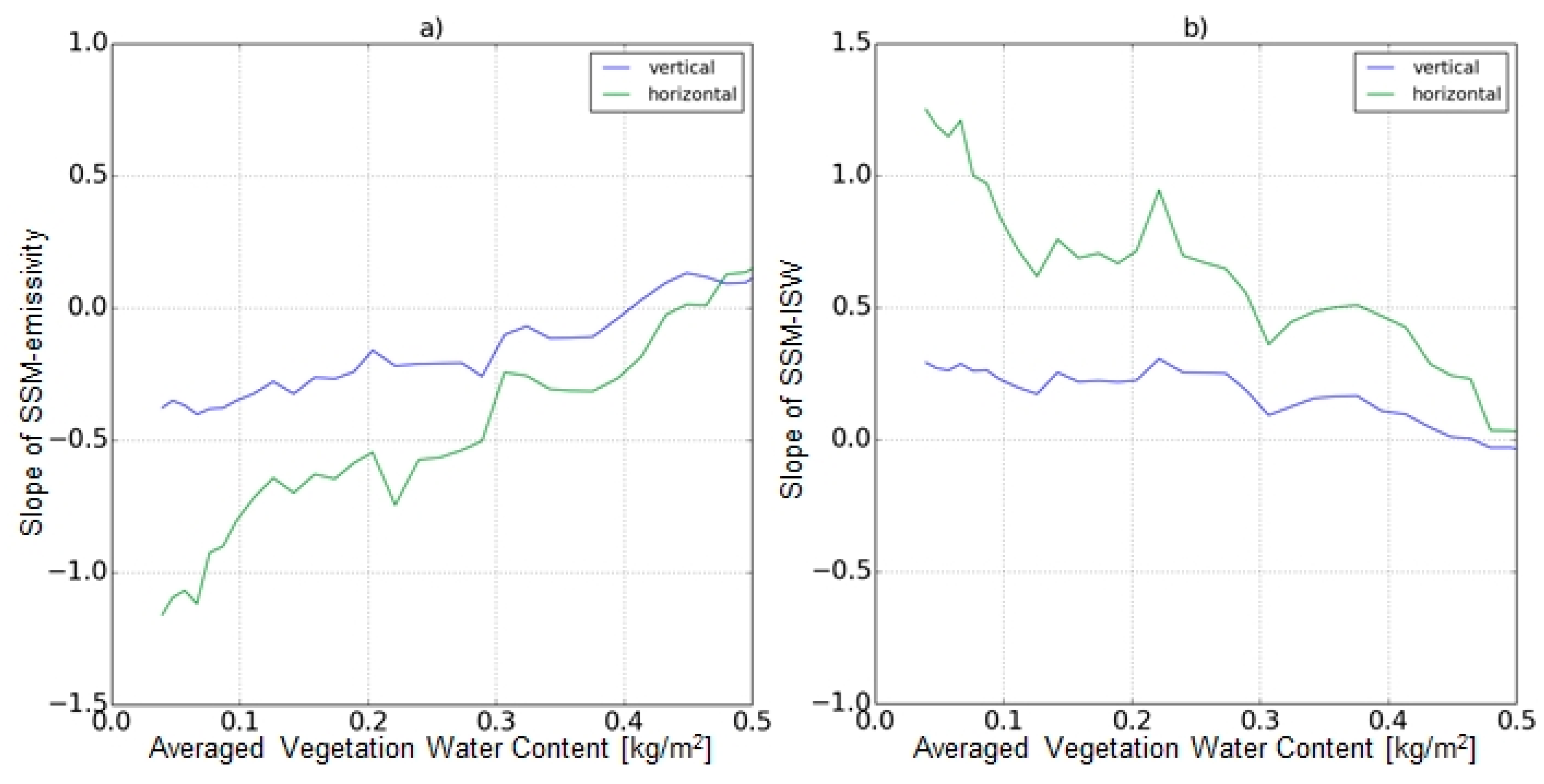
To further discuss the difficulty in detecting the signal of SSM under vegetation, we sorted every data according to their VWC values. Then we sampled 20 observations from the observation which has 1st smallest VWC to the observation which has 20th smallest VWC and calculate the slope of linear regression between SSM and emissivity on those 20 data. We performed the same analysis on the data from 2nd smallest VWC to 21st smallest VWC and then performed the analysis on the data from 3rd smallest VWC to 22nd smallest VWC. We iterated this process until all data is analyzed. Figure 9a shows the result of this iteration. In Figure 9a, the vertical axis indicates the slope of linear regression between SSM and emissivity in each group which has 20 observations while the horizontal axis indicates the averaged value of VWC among the 20 observations of each group. Theoretically, the emissivity decreases as SSM increases. We cannot find any negative slopes of the linear regressions if VWC is 0.5 (kg/m2) although some negative correlations can be found if VWC is less than 0.4 (kg/m2). The theoretical relationship between SSM and emissivity can be detected only when VWC is small in our ground truth.
Our sensitivity analysis shows that the uncertainty of surface soil roughness also makes it difficult to accurately retrieve SSM. Figure 8c,d show the sensitivity of RMS height to emissivity. As we discussed in the previous section, the increment of RMS height in the sensitivity analysis (=2 (mm)) is very small considering that we generally do not have the access to the a priori information of this parameter. In vertical polarization, the sensitivity of RMS height is similar to that of SSM. On the other hand, in horizontal polarization the sensitivity of RMS height is much larger than that of SSM. The horizontal emissivity varies more widely than the vertical emissivity, which is why horizontally polarized brightness temperature is often used for the retrieval algorithm [12]. However, the vertical polarized emissivity might be useful to minimize the effect of uncertainty of soil surface roughness.
The characteristic of the SSM-ISW relationship is similar to that of the SSM-emissivity relationship. Here we calculate ISW using 6.925 GHz and 36.5 GHz brightness temperatures. We cannot detect the strong correlation between SSM and ISW with a large amount of VWC (Figure 7e,g), which is consistent to the small sensitivity of SSM to ISW with VWC > 0.2 (kg/m2) in the LUT (Figure 8e,f). The observed ISW is weakly correlated to SSM with VWC < 0.2 (kg/m2) (Figure 7f,h). Theoretically, ISW increases as SSM increases. It becomes difficult to detect this positive correlation as VWC increases (Figure 9b). The effect of RMS height on ISW is significant and in horizontal polarization, the sensitivity of RMS height to ISW is larger than that of SSM (Figure 8g,h).
The performance of the LUT to reproduce observed ISW is limited. The RTM cannot reproduce the observed high ISW at both vertical and horizontal polarizations. The RTM of AIEM and the parameterization of dielectric constant by [33] cannot accurately simulate the emissivity of high frequencies (e.g., 36.5 GHz and 89 GHz) especially for horizontal polarization (Neluwara et al. in preparation). Since the calculation of ISW needs the brightness temperature of higher frequencies, the uncertainty of the RTM’s parameterizations in higher microwave frequencies degrades the simulation of ISW. Our in-situ observation suggests that there is much room for improvement of the RTM especially on horizontal polarized and higher frequency microwaves.
5. Discussion
In this paper, we provide the dataset of in-situ observed SSM, VWC, and brightness temperatures for a wide variety of plants: wheat, soybeans, corns, and olive trees. By analyzing this ground truth dataset and the result of numerical simulations, we support the following ideas about the uncertainty of SSM and VWC retrievals from passive microwave observations.
First, the PI-based algorithms to retrieve VOD and VWC are species-independent. Although this species’ independence has already been observed by [22], we increase the robustness of this theory by increasing the number of observations and including the observations of the olive trees. From short crops (soybeans) to tall trees (olives), the PI-VWC relationship is robust and we do not need to consider the effect of the difference of vegetation shape on microwave radiative transfer in the canopy at 6.925 GHz and 10.65 GHz as a first-order approximation. At 6.925 GHz, the upper limit of detectable VWC is approximately 1.5 (kg/m2).
Second, the uncertainty of surface soil roughness significantly degrades both SSM and VWC retrieval skills according to our analysis on numerical simulations. There are large sensitivities of RMS height to PI, emissivity, and ISW. Surface soil roughness is controlled by many factors and has large spatial and temporal variability. In this study, the field was randomly cultivated by a cultivator and hands, which brings a large spatial variability of surface soil roughness even in the small footprint of the GBMR. Surface soil roughness is also affected by wind and precipitation, which further brings spatial and temporal variability of surface soil roughness. In addition, sprouting from seed and the other ecosystem activities may contribute to change surface soil roughness. Many retrieval algorithms assume the fixed roughness parameters globally [15], and cannot address the effect of this surface soil roughness uncertainty. Some approaches to objectively determine the surface soil roughness parameters of RTM by introducing the visible/infrared observations (e.g., [21,22]) should be included to improve our VWC and SSM retrieval skills. In addition, our sensitivity analysis indicates that the vertically polarized brightness temperatures are less sensitive to surface soil roughness than the horizontally polarized brightness temperatures. In this study, we could not directly observe an accurate footprint-scale surface soil roughness since it is extremely difficult to correctly obtain the footprint scale roughness. The datasets of in-situ observations of surface soil roughness using laser scanning (e.g., [34,35]) should be provided in the future.
Third, at 6.925 GHz, SSM cannot be detected with VWC > 0.5 (kg/m2) and it is extremely difficult to detect SSM signals when VWC is larger than 0.2–0.3 (kg/m2). Since the emission from soil surface is disturbed by the vegetation canopy, it becomes difficult to detect the signal of surface emissions as VWC increases. In addition, the effect of RMS height on surface scattering strongly disturbs the relationship between SSM and surface emission. Therefore, we cannot detect any clear relationship between surface emission and SSM if VWC is more than 0.2–0.3 (kg/m2). This result is qualitatively consistent to Calvet et al. [36] in which a statistical soil moisture retrieval algorithm using C-band microwave field observations did not perform very well on a homogeneous wheat field with approximately 0–3 (kg/m2) VWC. The mission for AMSR-E was a root-mean-square error of 0.06 (m3/m3) soil moisture retrieval with VWC < 1.5 (kg/m2) [37] and the mission for AMSR2 is soil moisture retrieval with VWC < 2.0 (kg/m2). Based on our ground truth, these criteria seem to be too challenging. In many previous studies, however, SSM in moderately vegetated surfaces can be successfully retrieved from AMSR-E and AMSR2 brightness temperatures (e.g., [23]). Since there are many canopy openings in the large satellite footprint (>25 km), we may be able to retrieve SSM using the contribution of the emission from these canopy openings even if footprint-averaged VWC is large. Our results with the homogeneous footprints cannot be directly applied to the real world application in this aspect. In addition, in the real satellite applications, SSM and VWC (or VOD) are simultaneously retrieved although we analyzed the performances of indices sensitive to SSM and VWC individually. The effect of the simultaneous use of the indices has not been included in the analysis of this paper.
Fourth, the LUT generated by AIEM and tau-omega model includes almost all of our in-situ observations, which means the state-of-the-art RTM can accurately predict our in-situ observed microwave radiative transfer. However, the RTM may have some biases in the simulation of higher frequencies. Improving this part of the RTM to accurately simulate ISW should be our future work.
Please note that the findings of this paper cannot be directly applied to the SSM and VWC retrievals based on L-band microwave observations. Sensitivity of brightness temperature to SSM, VWC, and the other land surface variables strongly depends on a microwave frequency used. We recommend to implement a long-term observation campaign with a similar observation design to this study in order to quantitatively discuss the capability and limitation of the retrieval algorithms used for Soil Moisture and Ocean Salinity (SMOS) and Soil Moisture Active Passive (SMAP).
6. Conclusions
In this paper, we provided the new in-situ observation dataset which is useful to evaluate the capability and limitation of the SSM and VWC retrieval algorithms based on microwave radiometry. Since the dataset is available as a Supplementary Material of this paper (Data S1), we expect that the new-insitu observation dataset is the useful benchmark for both developers and users of SSM and VWC products retrieved by passive microwave remote sensing. By analyzing this dataset as well as the simulation by the RTM, we obtained several findings related to the capability and limitation of the current AMSR-E/AMSR2 SSM and VWC retrieval algorithms. First, C-band microwave radiative transfer in canopy is species-independent as a first-order approximation. Current algorithms which do not explicitly consider the diversity of the vegetation structure are reasonable. Second, the uncertainty of surface soil roughness significantly degrades the retrieval skills so that technique to eliminate the effect of surface soil roughness uncertainty is urgently needed. Third, SSM cannot be detected with VWC > 0.5 (kg/m2) by AMSR-E/AMSR2 observations if the footprint is homogeneously vegetated. It should be noted that the current performance of satellite SSM products in a vegetated area may be strongly influenced by the contribution of canopy openings in the large satellite footprint. Considering microwave satellite based SSM retrieval as a mixed picture problem is important. Fourth, the LUT generated by the RTM can accurately predict our in-situ observations. The AIEM and tau-omega model is the suitable model for SSM and VWC retrievals.
Supplementary Materials
The following are available online at www.mdpi.com/2072-4292/9/7/655/s1.
Acknowledgments
Yohei Sawada has been supported by Japan Society of Promotion of Science (JSPS) (255893). This study is funded by Japan Aerospace eXploration Agency (JAXA), the Research Program on Climate Change Adaptation (RECCA), and JSPS KAKENHI Grant Number JP17K18352. We thank Mohamed Rasmy, Rie Seto, Panduka Neluwala, Kinya Toride, Martin Gomez Garcia, Huiyu Bao, Weiqiang Ma, Yushi Suzuki, Peter Lawford, Seemanta Bhagabati, Ralph Achierto, Katsunori Tamagawa and Atsushi Yamamoto for helping our field work. We appreciate the staffs at the Institute for Sustainable Agro-ecosystem Services, Graduate School of Agriculture, the University of Tokyo, for their support to maintain the observation site.
Author Contributions
All authors, Y.S., H.T., and T.K. contributed to design the study. Y.S. and H.T. performed the field experiment. Y.S. performed numerical experiments, analyzed the data and wrote the initial version of the paper. T.K. was the PI and lead the project. All authors, Y.S., H.T., and T.K. contributed to edit and discussed the contents of the paper.
Conflicts of Interest
The authors declare no conflict of interest.
References
- Anderson, W.B.; Zaitchik, B.F.; Hain, C.R.; Anderson, M.C.; Yilmaz, M.T.; Mecikalski, J.; Schultz, L. Towards an integrated soil moisture drought monitor for East Africa. Hydrol. Earth Syst. Sci. 2012, 16, 2893–2913. [Google Scholar] [CrossRef]
- Taylor, C.M.; de Jeu, R.A.M.; Guichard, F.; Harris, P.P.; Dorigo, W.A. Afternoon rain more likely over drier soils. Nature 2012, 489, 423–426. [Google Scholar] [CrossRef] [PubMed]
- Liu, Y.Y.; van Dijk, A.I.J.M.; de Jeu, R.A.M.; Canadell, J.G.; McCabe, M.F.; Evens, J.P.; Wang, G. Recent reversal in loss of global terrestrial biomass. Nat. Clim. Chang. 2015, 5, 470–474. [Google Scholar] [CrossRef]
- Zhou, L.; Tian, Y.; Myneni, R.B.; Ciais, P.; Saatchi, S.; Liu, Y.Y.; Piao, S.; Chen, H.; Vermote, E.F.; Song, C.; et al. Widespread decline of Congo rainforest greenness in the past decade. Nature 2014, 509, 86–90. [Google Scholar] [CrossRef] [PubMed]
- Walker, J.P.; Houser, P.R. A methodology for initializing soil moisture in a global climate model: Assimilation of near-surface soil moisture observations. J. Geophys. Res. Atmos. 2001, 106, 11761–11774. [Google Scholar] [CrossRef]
- Yang, K.; Watanabe, T.; Koike, T.; Li, X.; Fujii, H.; Tamagawa, K.; Ma, Y.; Ishikawa, H. Auto-calibration System Developed to Assimilate AMSR-E Data into a Land Surface Model for Estimating Soil Moisture and the Surface Energy Budget. J. Meteorol. Soc. Jpn. 2007, 85A, 229–242. [Google Scholar] [CrossRef]
- Rasmy, M.; Koike, T.; Boussetta, S.; Lu, H.; Li, X. Development of a Satellite Land Data Assimilation System Coupled With a Mesoscale Model in the Tibetan Plateau. IEEE Trans. Geosci. Remote Sens. 2011, 49, 2847–2862. [Google Scholar] [CrossRef]
- Sawada, Y.; Koike, T. Simultaneous estimation of both hydrological and ecological parameters in an ecohydrological model by assimilating microwave signal. J. Geophys. Res. Atmos. 2014, 119. [Google Scholar] [CrossRef]
- Sawada, Y.; Koike, T.; Walker, J.P. A land data assimilation system for simultaneous simulation of soil moisture and vegetation dynamics. J. Geophys. Res. Atmos. 2015, 120. [Google Scholar] [CrossRef]
- Sawada, Y.; Koike, T. Towards ecohydrological drought monitoring and prediction using a land data assimilation system: A case study on the Horn of Africa drought (2010–2011). J. Geophys. Res. Atmos. 2016, 121, 8229–8242. [Google Scholar] [CrossRef]
- Lu, H.; Yang, K.; Koike, T.; Zhao, L.; Qin, J. An improvement of the radiative transfer model component of a land data assimilation system and its validation on different land characteristics. Remote. Sens. 2015, 7, 6358–6379. [Google Scholar] [CrossRef]
- Owe, M.; de Jeu, R.; Walker, J. A methodology for surface soil moisture and vegetation optical depth retrieval using the microwave polarization difference index. IEEE Trans. Geosci. Remote Sens. 2001, 39, 1643–1654. [Google Scholar] [CrossRef]
- Njoku, E.G.; Jackson, T.J.; Lakshmi, V.; Chan, T.K.; Nghiem, S.V. Soil Moisture Retrieval From AMSR-E. IEEE Trans. Geosci. Remote Sens. 2003, 41, 215–229. [Google Scholar] [CrossRef]
- Koike, T.; Nakamura, Y.; Kaihotsu, I.; Davva, G.; Matsuura, N.; Tamagawa, K.; Fujii, H. Development of an Advanced Microwave Scanning Radiometer (AMSR-E) Algorithm of Soil Moisture and Vegetation Water Content. Ann. J. Hydraul. Eng. 2004, 48, 217–222. (In Japanese) [Google Scholar] [CrossRef]
- Fujii, H.; Koike, T.; Imaoka, K. Improvement of the AMSR-E Algorithm for Soil Moisture Estimation by Introducing a Fractional Vegetation Coverage Dataset Derived from MODIS Data. J. Remote Sens. Soc. Jpn. 2009, 29, 282–292. [Google Scholar]
- Ulaby, F.; Moore, R.K.; Fung, A. Microwave Remote Sensing: Active and Passive—Volume Scattering and Emission Theory; Artech House: Dedham, MA, USA, 1986. [Google Scholar]
- Kuria, D.N.; Koike, T.; Lu, H.; Tsutsui, H.; Graf, T. Field-Supported Verification and Improvement of a Passive Microwave Surface Emission Model for Rough, Bare and Wet Soil Surfaces by Incorporating Shadowing Effects. IEEE Trans. Geosci. Remote Sens. 2007, 45, 1207–1216. [Google Scholar] [CrossRef]
- Mo, T.; Choudhury, B.J.; Schmugge, T.J.; Wang, J.R.; Jackson, T.J. A Model for Microwave Emission From Vegetation-Covered Fields. J. Geophys. Res. 1982, 87, 11229–11237. [Google Scholar] [CrossRef]
- Paloscia, S.; Pampaloni, P. Microwave polarization index for monitoring vegetation growth. IEEE Trans. Geosci. Remote Sens. 1988, 26, 617–621. [Google Scholar] [CrossRef]
- Holmes, T.R.H.; De Jeu, R.A.M.; Owe, M.; Dolman, A.J. Land surface temperature from Ka band (37 GHz) passive microwave observations. J. Geophys. Res. 2009, 114, D04113. [Google Scholar] [CrossRef]
- Wang, S.; Wigneron, J.P.; Jiang, L.M.; Parrens, M.; Yu, X.Y.; Al-Yaari, A.; Ye, Q.Y.; Fernandez-Moran, R.; Ji, W.; Kerr, Y. Global-Scale Evaluation of Roughness Effects on C-Band AMSR-E Observations. Remote Sens. 2015, 7, 5734–5757. [Google Scholar] [CrossRef]
- Sawada, Y.; Tsutsui, H.; Koike, T.; Rasmy, M.; Seto, R.; Fujii, H. A field verification of an algorithm for retrieving vegetation water content from passive microwave observations. IEEE Trans. Geosci. Remote Sens. 2016, 54, 2082–2095. [Google Scholar] [CrossRef]
- Jackson, T.J.; Cosh, M.H.; Bindlish, R.; Starks, P.J.; Bosch, D.D.; Seyfried, M.; Goodrich, D.C.; Moran, M.S.; Du, J. Validation of Advanced Microwave Scanning Radiometer Soil Moisture Products. IEEE Trans. Geosci. Remote Sens. 2010, 48, 4256–4272. [Google Scholar] [CrossRef]
- Patton, J.; Hornbuckle, B. Initial Validation of SMOS Vegetation Optical Thickness in Iowa. IEEE Trans. Geosci. Remote Sens. Lett. 2013, 42, 647–651. [Google Scholar] [CrossRef]
- Crow, W.T.; Chan, S.T.K.; Entekhabi, D.; Houser, P.R.; Hsu, A.Y.; Jackson, T.J.; Njoku, E.G.; O’Nell, P.E.; Shi, J.; Zhan, X. An observing system simulation experiment for Hydros radiometer-only soil moisture products. IEEE Trans. Geosci. Remote Sens. 2005, 43, 1289–1303. [Google Scholar] [CrossRef]
- Zhan, X.; Crow, W.T.; Jackson, T.J.; O’Nell, P.E. Improving spaceborne radiometer soil moisture retrievals with alternative aggregation rules for ancillary parameters in highly heterogeneous vegetated areas. IEEE Trans. Geosci. Remote Sens. Lett. 2008, 5, 261–265. [Google Scholar] [CrossRef]
- Neelam, M.; Mohanty, B.P. Global sensitivity analysis of the radiative transfer model. Water Resour. Res. 2015, 51, 2428–2443. [Google Scholar] [CrossRef]
- Jackson, T.J.; Schmmuge, T.J. Vegetation effects on the microwave emission of soils. Remote Sens. Environ. 1991, 36, 203–212. [Google Scholar] [CrossRef]
- Owe, M.; de Jeu, R.; Holmes, T. Multisensor historical climatology of satellite-derived global land surface moisture. J. Geophys. Res. 2008, 113, F01002. [Google Scholar] [CrossRef]
- Paloscia, S.; Pampaloni, P. Microwave vegetation indexes for detecting biomass and water conditions of agricultural crops. Remote Sens. Environ. 1992, 40, 15–26. [Google Scholar] [CrossRef]
- Ferrazzoli, P.; Guerriero, L.; Paloscia, S.P.; Pampaloni, P. Modeling Polarization Properties of Emission from Soil Covered with Vegetation. IEEE Trans. Geosci. Remote Sens. 1992, 30, 157–165. [Google Scholar] [CrossRef]
- Chen, K.; Wu, T.D.; Tsang, L.; Li, Q.; Shi, J.C.; Fung, A.K. The emission of rough surfaces calculated by the integral equation method with a comparison to a three dimensional moment method simulation. IEEE Trans. Geosci. Remote Sens. 2001, 38, 249–256. [Google Scholar] [CrossRef]
- Dobson, D.M.; Ulaby, F.; Hallikainen, M.; El-Rayes, M. Microwave dielectric behavior of wet soil—Part II: Dielectric mixing models. IEEE Trans. Geosci. Remote Sens. 1985, 23, 35–46. [Google Scholar] [CrossRef]
- Haubrock, S.N.; Kuhnert, M.; Chabrillat, S.; Guntner, A.; Kaufmann, H. Spatiotemporal variations of soil surface roughness from in-situ laser scanning. Catena 2009, 79, 128–139. [Google Scholar] [CrossRef]
- Alvarez-Mozos, J.; Verhoest, N.E.C.; Larranaga, A.; Casali, J.; Gonzalez-Audicana, M. Influence of surface roughness spatial variability and temporal dynamics on the retrieval of soil moisture from SAR observations. Sensors 2009, 9, 463–489. [Google Scholar] [CrossRef] [PubMed]
- Calvet, J.C.; Wigneron, J.P.; Walker, J.; Karbou, F.; Chanzy, A.; Albergel, C. Sensitivity of Passive Microwave Observations to Soil Moisture and Vegetation Water Content: L-Band to W-Band. IEEE Trans. Geosci. Remote Sens. 2011, 49, 1190–1199. [Google Scholar] [CrossRef]
- Shibata, A.; Imaoka, K.; Koike, T. AMSR/AMSR-E level 2 and 3 algorithm developments and data validation plans of NASDA. IEEE Trans. Geosci. Remote Sens. 2003, 41, 195–203. [Google Scholar] [CrossRef]
Figure 1.
Ground-based microwave radiometer.
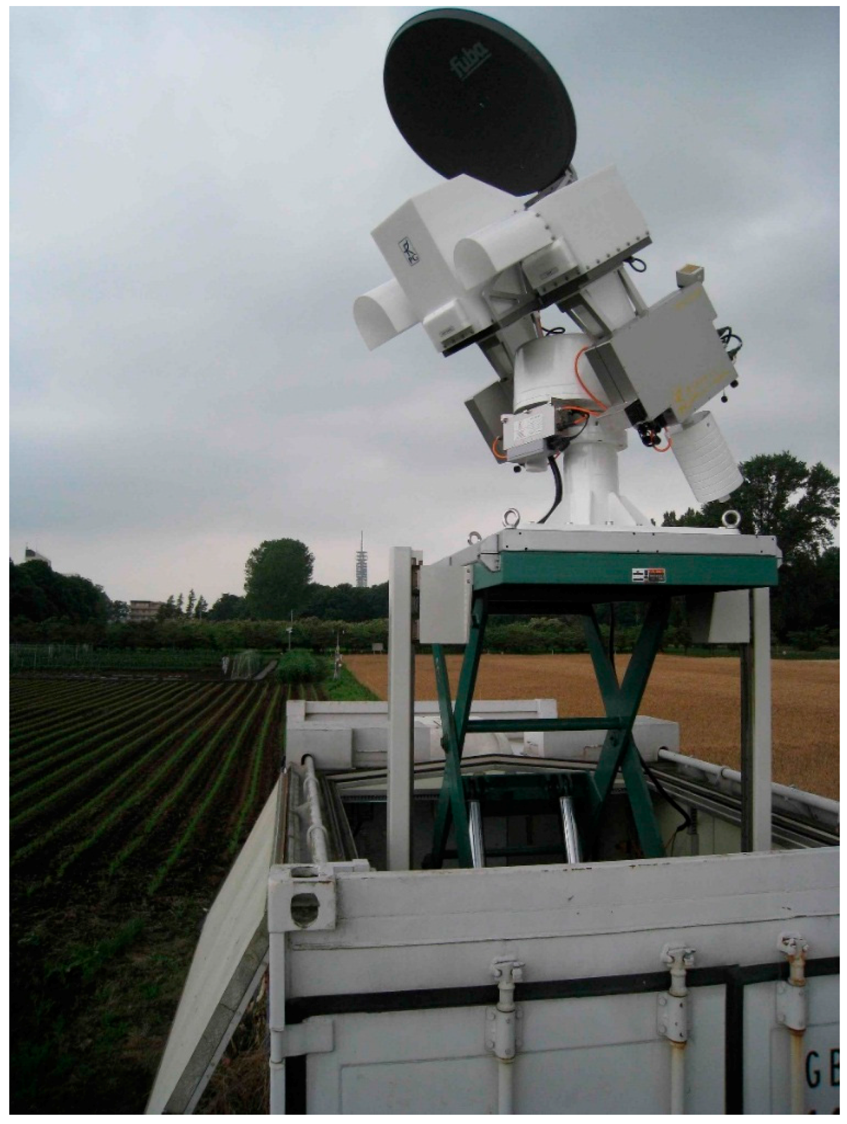
Figure 2.
Condition of footprints of (a) Phase I, (b) Phase II, (c) Phase III, (d) Phase IV, and (e) Phase V (see also Table 1).
Figure 2.
Condition of footprints of (a) Phase I, (b) Phase II, (c) Phase III, (d) Phase IV, and (e) Phase V (see also Table 1).

Figure 3.
Diversity of the structures of the observed vegetation. (a) Relationship between dry mass and vegetation water content. (b) Relationship between vegetation water content in leaf and stem. (c) Relationship between vegetation water content and leaf area index.
Figure 3.
Diversity of the structures of the observed vegetation. (a) Relationship between dry mass and vegetation water content. (b) Relationship between vegetation water content in leaf and stem. (c) Relationship between vegetation water content and leaf area index.

Figure 4.
(a) Relationship between the observed 37 GHz vertical polarized brightness temperatures (TB) and the observed ground physical temperatures. Dashed line is the empirical relationship proposed by Holmes et al., 2008. (b) The difference between the physical temperature of the lookup table (293 (K)) and the physical temperature estimated by the empirical relationship of Holmes et al., 2008 using the 37 GHz vertical polarized brightness temperatures of the lookup table. Surface soil moisture, vegetation water content, and RMS height are set to 0.25 (m3/m3), 2.0 (kg/m2), and 0.1 (cm), respectively.

Figure 5.
Relationship between vegetation water content and polarization index at (a) 6.925 GHz and (b) 10.65 GHz. Gray dots are the dataset of the lookup table. We show the lookup table with every other bin for single scattering albedos and a RMS height for brevity.
Figure 5.
Relationship between vegetation water content and polarization index at (a) 6.925 GHz and (b) 10.65 GHz. Gray dots are the dataset of the lookup table. We show the lookup table with every other bin for single scattering albedos and a RMS height for brevity.

Figure 6.
(a) Sensitivity of vegetation water content to PI as a function of RMS height and vegetation water content (surface soil moisture, vertical and horizontal single scattering albedos are set to 0.30 (m3/m3), 0.04, and 0.04, respectively). (b) Same as (a) but as a function of surface soil moisture and vegetation water content (RMS height, vertical and horizontal single scattering albedos are set to 0.1 (cm), 0.04, and 0.04, respectively). (c) Sensitivity of RMS height to PI as a function of RMS height and vegetation water content (surface soil moisture, vertical and horizontal single scattering albedos are set to 0.30 (m3/m3), 0.04, and 0.04, respectively). (d) Sensitivity of SSM to PI as a function of surface soil moisture and vegetation water content (RMS height, vertical and horizontal single scattering albedos are set to 0.1 (cm), 0.04, and 0.04, respectively).

Figure 7.
(a–d) Relationship between the surface soil moisture and the emissivity at (a,b) vertical polarized and (c,d) horizontal polarized 6.925 GHz microwave. (a,c) show every plot while (b,d) show the plots with vegetation water content less than 0.20 [kg/m3]. (e–h) same as (a–d) but for ISW. Gray dots are the dataset of the lookup table. We show the lookup table with every other bin for single scattering albedos and a RMS height for brevity.
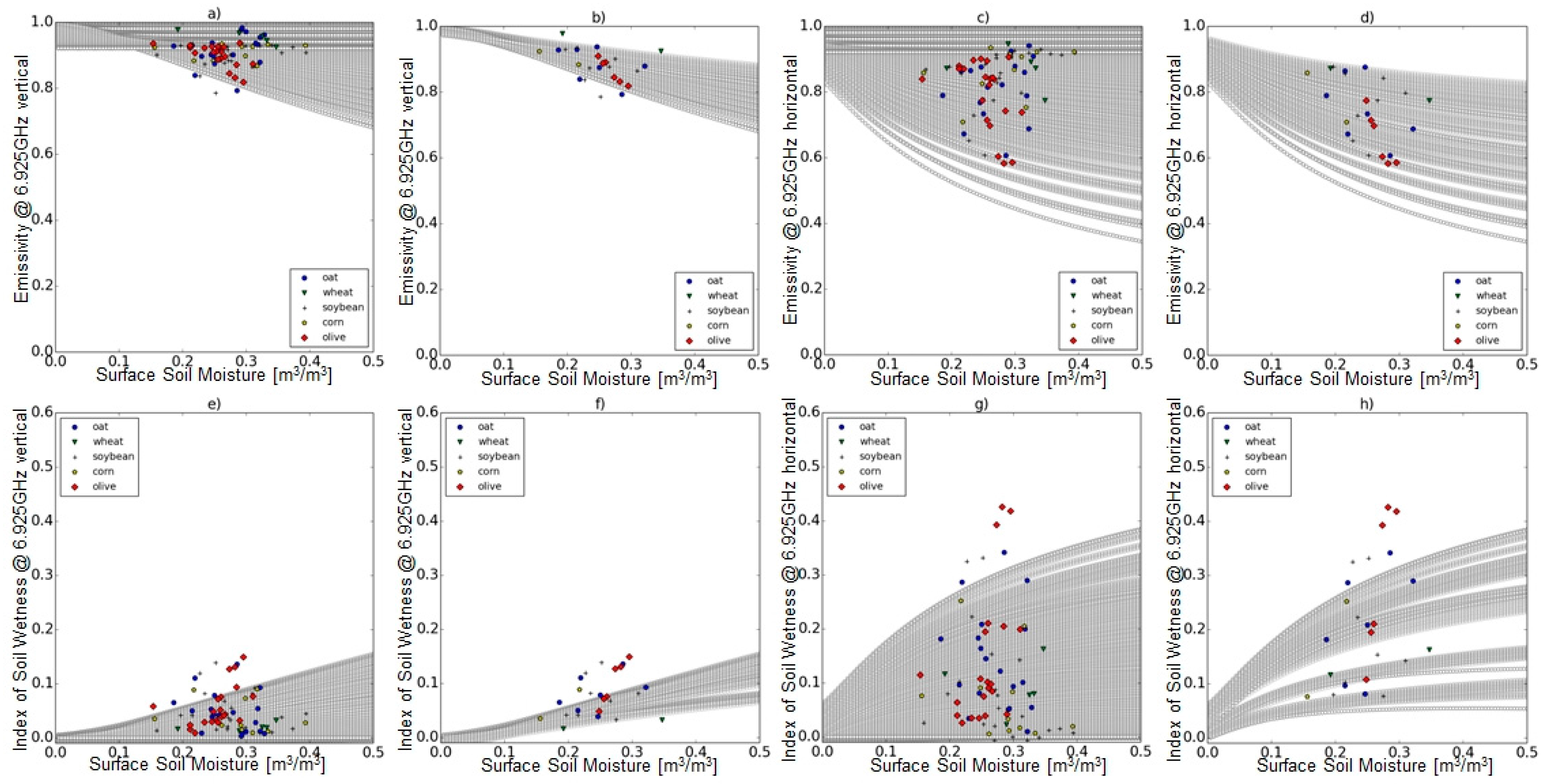
Figure 8.
(a,b) Sensitivity of surface soil moisture to emissivity of (a) vertical polarized and (b) horizontal polarized microwave as a function of surface soil moisture and vegetation water content (RMS height, vertical and horizontal single scattering albedos are set to 0.1 (cm), 0.04, and 0.04, respectively). (c,d) Sensitivity of RMS height to emissivity of (c) vertical polarized and (d) horizontal polarized microwave as a function of RMS height and vegetation water content (surface soil moisture, vertical and horizontal single scattering albedos are set to 0.3 (m3/m3), 0.04, and 0.04, respectively). (e,f) Same as (a,b) but for ISW. (g,h) Same as (c,d) but for ISW.
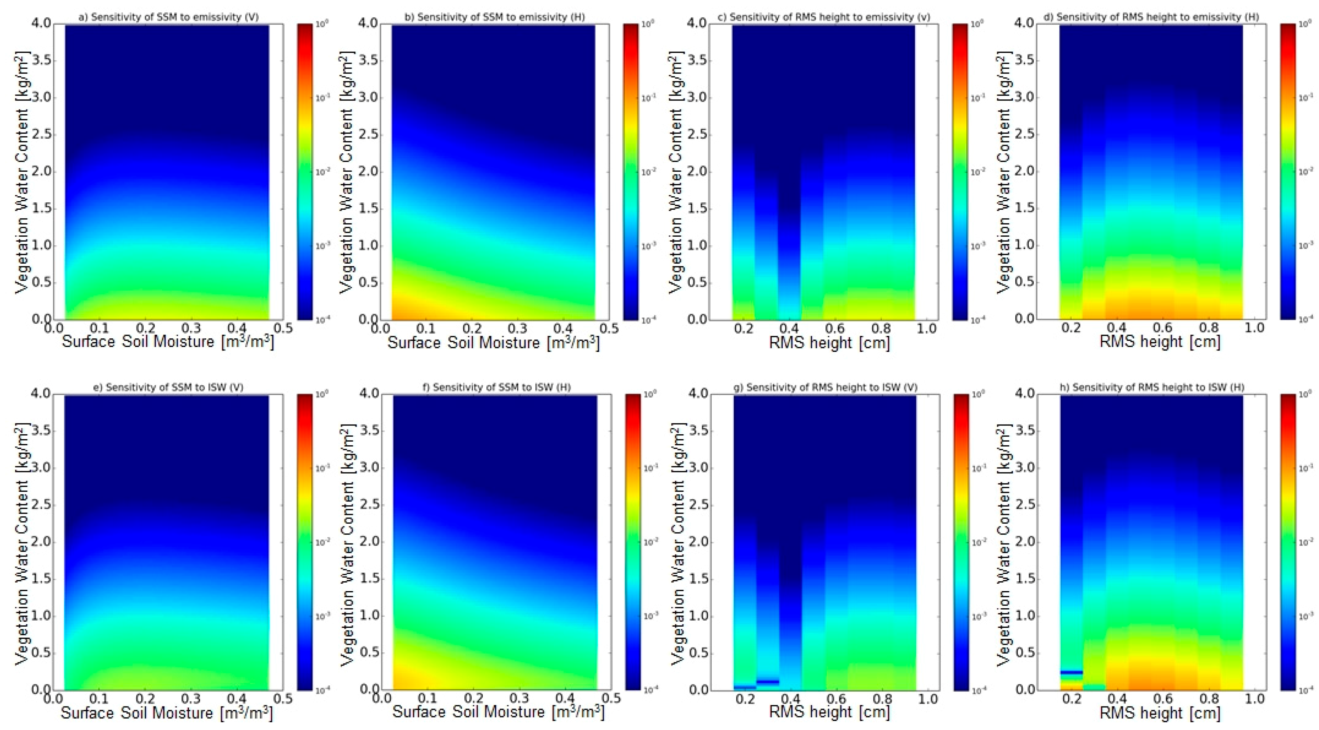
Figure 9.
Slope of the linear regression between (a) 6.925 GHz emissivity and surface soil moisture, and (b) 6.925 GHz and 37 GHz ISW and surface soil moisture as a function of averaged vegetation water content among 20 observations sampled from our in-situ observations. Blue and green lines show the results of vertical polarized and horizontal polarized microwave, respectively. See manuscript for the details of this analysis.

Table 1.
Observation schedule.
| Phase | Observed Plant(s) | Period |
|---|---|---|
| I | Oat | June 2012–September 2012 |
| II | Wheat | December 2012–June 2013 |
| III | Corn & Soybean | August 2013–December 2013 |
| IV | Oat & Soybean | May 2014–June 2014 |
| V | Olive | August 2015–February 2016 |
Table 2.
List of inputs/parameters of the RTM to generate the lookup table.
| Type | Name | Value (s) | # of Bins | Intervals of Two Bins | Increment (Δ in Equation (7)) |
|---|---|---|---|---|---|
| variable in LUT | Surface soil moisture (m3/m3) | 0.005–0.5 | 100 | 0.005 | 10 |
| Vegetation water content (kg/m2) | 0.0–4.0 | 100 | 0.04 | 10 | |
| Single scattering albedo (vertical) | 0.0–0.09 | 10 | 0.01 | 2 | |
| Single scattering albedo (horizontal) | 0.0–0.09 | 10 | 0.01 | 2 | |
| RMS height of soil surface (cm) | 0.1–1.0 | 10 | 0.1 | 2 | |
| Invariable in LUT | Wavelength-independent parameter of VOD-VWC relationship (b’) | 0.5 | |||
| Wavelength-dependent parameter of VOD-VWC relationship (χ) | −1.0 | ||||
| Correlation length of soil surface (cm) | 1.5 | ||||
| Physical Temperature (K) | 293 |
© 2017 by the authors. Licensee MDPI, Basel, Switzerland. This article is an open access article distributed under the terms and conditions of the Creative Commons Attribution (CC BY) license (http://creativecommons.org/licenses/by/4.0/).
Share and Cite
MDPI and ACS Style
Sawada, Y.; Tsutsui, H.; Koike, T. Ground Truth of Passive Microwave Radiative Transfer on Vegetated Land Surfaces. Remote Sens. 2017, 9, 655. https://doi.org/10.3390/rs9070655
AMA Style
Sawada Y, Tsutsui H, Koike T. Ground Truth of Passive Microwave Radiative Transfer on Vegetated Land Surfaces. Remote Sensing. 2017; 9(7):655. https://doi.org/10.3390/rs9070655
Chicago/Turabian StyleSawada, Yohei, Hiroyuki Tsutsui, and Toshio Koike. 2017. "Ground Truth of Passive Microwave Radiative Transfer on Vegetated Land Surfaces" Remote Sensing 9, no. 7: 655. https://doi.org/10.3390/rs9070655
Note that from the first issue of 2016, this journal uses article numbers instead of page numbers. See further details here.