Estimation of FAPAR over Croplands Using MISR Data and the Earth Observation Land Data Assimilation System (EO-LDAS)

Abstract

The Fraction of Absorbed Photosynthetically-Active Radiation (FAPAR) is an important parameter in climate and carbon cycle studies. In this paper, we use the Earth Observation Land Data Assimilation System (EO-LDAS) framework to retrieve FAPAR from observations of directional surface reflectance measurements from the Multi-angle Imaging SpectroRadiometer(MISR) instrument. The procedure works by interpreting the reflectance data via the semi-discrete Radiative Transfer (RT) model, supported by a prior parameter distribution and a dynamic regularisation model and resulting in an inference of land surface parameters, such as effective Leaf Area Index (LAI), leaf chlorophyll concentration and fraction of senescent leaves, with full uncertainty quantification. The method is demonstrated over three agricultural FLUXNET sites, and the EO-LDAS results are compared with eight years of in situ measurements of FAPAR and LAI, resulting in a total of 24 site years. We additionally compare three other widely-used EO FAPAR products, namely the MEdium Resolution Imaging Spectrometer (MERIS) Full Resolution, the MISR High Resolution (HR) Joint Research Centre Two-stream Inversion Package (JRC-TIP) and MODIS MCD15 FAPAR products. The EO-LDAS MISR FAPAR retrievals show a high correlation with the ground measurements ($r^2$ > 0.8), as well as the lowest average $RMSE$ (0.14), in line with the MODIS product. As the EO-LDAS solution is effectively interpolated, if only measurements that are coincident with MISR observations are considered, the correlation increases ($r^2$ > 0.85); the $RMSE$ is lower by 4–5%; and the bias is 2% and 7%. The EO-LDAS MISR LAI estimates show a strong correlation with ground-based LAI (average $r^2$ = 0.76), but an underestimate of LAI for optically-thick canopies due to saturation (average $RMSE$ = 2.23). These results suggest that the EO-LDAS approach is successful in retrieving both FAPAR and other land surface parameters. A large part of this success is based on the use of a dynamic regularisation model that counteracts the poor temporal sampling from the MISR instrument.

1. Introduction

The Fraction of Absorbed Photosynthetically-Active Radiation (FAPAR) is recognised as an essential climate variable, and it plays an important role in biosphere and climate modelling [1]. FAPAR is defined as incident solar radiation in the range 400–700 nm that is absorbed by the photosynthetic tissue of canopy [2] and, thus, is an important control on the photosynthetic activity of vegetation. FAPAR has been widely used for monitoring drought, biodiversity, land degradation, phenology, CO${}_2$ emission studies and Dynamic Global Vegetation Models (DGVM) [3,4,5,6,7,8]. Although we consider FAPAR to be a land surface parameter (e.g., only related to the land), the amount of direct and diffuse radiation affects its value [9,10].

In order to infer the state of the land surface, the inversion of physically-based models that describe the interaction of incoming radiation with the soil-leaf-canopy medium, typically based on radiative transfer (RT) theory, are generally used [11,12]. The main benefits of using physically-based RT models is their ability to cope with different sensor properties (angular and spectral sampling characteristics, etc.) and that they are more generic than empirical approaches, as they incorporate basic physical laws (e.g., energy conservation) that are universally applicable, and should result in a more robust interpretation of the measurements. The retrieval of land surface parameters using RT models is complicated by the problem being `ill-posed’ [13]. A well-posed problem is one that has a solution; the solution is unique and changes continuously with changing input. A problem that does not hold these conditions is an ill-posed problem [14]. In the context of EO, it often means that an infinite number of land surface parametrisations results in equally likely predictions of the observations. Here, we can see “inputs” as the inputs to RT model, i.e., state variables (LAI, chlorophyll, leaf water content, etc.). One of the possible solutions for improving the situation is using a priori knowledge, such as physically-realistic parameter distributions and/or constraints on parameter smoothness (e.g., in time, space) [15,16]. In practice, ill-posedness means that retrieved parameters have very large uncertainties. Prior information restricts the possible space of potential solutions. This strategy is deployed by the Joint Research Centre Two-Stream Inversion Package (JRC-TIP) product [17]. Other sources of uncertainty in the retrievals arise from sparse observations, e.g., due to cloudiness or orbital and sensor design characteristics. These problems call for a credible and traceable uncertainty quantification framework that allows users to understand shortcomings in the inverted data.

A final comment on FAPAR products is that its magnitude is closely related to other biophysical properties, such as Leaf Area Index (LAI), leaf optical properties, single scattering albedo, etc. These parameters are often derived independently from the same original datasets in RT model inversion schemes, making a number of assumptions on, e.g., canopy structure, leaf optical properties, etc., that might result in inconsistencies between derived products’ datasets.

In order to meet the requirements described above, this paper explores the use of the Earth Observation Land Data Assimilation System (EO-LDAS), a general purpose Data Assimilation (DA) framework, to invert a time series of surface directional reflectance observations from the Moderate-resolution Imaging Spectroradiometer (MODIS) and Multi-angle Imaging SpectroRadiometer (MISR) sensors to infer land surface parameters. We use these parameters (and associated uncertainties) to provide a consistent estimation of FAPAR. The results are compared with other products available over the same sites. Two recent papers provide an approachable and non-specialist overview of this area [18,19].

EO-LDAS is a system that allows interpreting spectral observations to provide an optimal quantitative estimate of the Earth surface state. It permits the combination of observations from different sensors despite differences in spatial and spectral resolution and acquisition frequencies. EO-LDAS is based on variational DA and uses physically-based RT modes to map from state (LAI, leaf and soil optical properties, for example) to observation space (in this case, surface directional reflectance). EO-LDAS essentially allows a flexible description of both the `fit to the observations’ using RT models and the prior information, either as parameter distributions, or temporal, or spatial regularisation constraints.

Previous EO-LDAS results have been validated using synthetic Sentinel-2 data [16,20]. In [21], emulators (fast surrogate approximations to computationally-expensive physical RT models) are demonstrated within the EO-LDAS framework, showing that the addition of a simple regularisation dynamic model results in improved retrievals in a synthetic example that combines observations from Sentinel-2/MSI, Sentinel-3/SLSTR and Proba-V observations. In all of these studies, the authors found that adding temporal regularisation as an additional prior constraint resulted in a significant reduction of uncertainty in the estimates of the inferred land surface parameters. Here, we analyse the results of EO-LDAS temporal regularization with MISR observations by comparing them against ground-based FAPAR estimated over an agricultural test site [22] and against MEdium Resolution Imaging Spectrometer (MERIS) FAPAR at 300 m, MISR High Resolution (HR) JRC-TIP and MODIS MOD15 [23] products for 2001–2008.

Multi-angular remote sensing of the land surface can help to reveal structural properties of the vegetation and thus to improve characterisation of the vegetation cover [24]. Three widely-used instruments provide multi-angular information at the global scale: Polarization and Directionality of Earth Reflectance (POLDER) [25], Sea and Land Surface Temperature Radiometer (SLSTR) [26] and MISR [27]. MISR has nine cameras pointed to directions from −70${}^{°}$–70${}^{°}$, four spectral bands from blue to near-infrared and spatial resolution at 275 m for the nadir camera and red band and at 1.1 km for others. A number of studies has demonstrated that exploiting multi-angular information of MISR can improve retrieval of LAI and FAPAR [28,29,30,31]. One physically-based approach for deriving FAPAR from 275 m is the JRC-TIP approach that uses MISR resolution data [32,33] to invert a radiative transfer model. This package is based on a two-stream model [34] and uses prior information to constrain the RT model inversion. In addition, this application provides information about theoretical uncertainties for both output state parameters and output fluxes. JRC-TIP output was tested against independent parameter estimates over a range of different areas [17,35].

The next sections describe the test site, EO data and FAPAR retrieval algorithms with their respective definition and assumptions. Following this, we present a short summary of the theoretical basis of EO-LDAS and FAPAR estimation. We then present the retrieved values from EO-LDAS and proceed to compare them with ground measurements. We also show and discuss comparisons with other products and discuss these comparisons. We finally draw some conclusions.

2. Materials

2.1. Test Site Description and Ground-Based Data Collection

The study area is comprised of the three agricultural FLUXNET sites, US-Ne1 (41.165${}^{°}$N, 96.477${}^{°}$W), US-Ne2 (41.1649${}^{°}$N, 96.470${}^{°}$W) and US-Ne3 (41.1797${}^{°}$N, 96.4730${}^{°}$W) (http://fluxnet.orn.gov) located at the Lincoln Agricultural Research and Development Center near Mead (NE, USA) (Figure 1). Each field has an area of approximately 65 ha. The US-Ne1 site was cultivated with maize from 2001–2008. The sites US-Ne2 and US-Ne3 were cultivated with maize in 2001, 2003, 2005 and 2007 and with soy bean in 2002, 2004, 2006 and 2008 [22,36]. Fields US-Ne1 and US-Ne2 are irrigated, and US-Ne3 is rainfed. The growing season is approximately from May–October.

In situ measurements of FAPAR were carried out from 2001–2008 between June and September/October with an interval of 2–6 days. These measurements were performed with a Li-Cor quantum sensor (LI-COR Inc., Lincoln, NE, USA) by detecting incoming photosynthetically active radiation ($PA{R}_{inc}$), PAR reflected by the canopy and soil ($PA{R}_{out}$), PAR transmitted through the canopy ($PA{R}_{transm}$) and PAR reflected by the soil ($PA{R}_{soil}$) (Equation (1)) [36].

$$FAPA{R}_{total}=\frac{PA{R}_{inc}-PA{R}_{out}-PA{R}_{transm}+PA{R}_{soil}}{PA{R}_{inc}}$$

(1)

Hourly values of radiation measured throughout a day were integrated in order to get daily values when $PA{R}_{inc}$ was >1 μmolm⁻²s⁻¹ [22]. A detailed description of the measurements protocols can be found in [22,36]. In summary, the authors obtain the absorption PAR for only green elements, i.e., $FAPA{R}_{green}$, with the following correction for which $LA{I}_{green}$ and $LA{I}_{total}$ have been measured through a destructive determination technique:

$$FAPA{R}_{green}=FAPA{R}_{total}\frac{LA{I}_{green}}{LA{I}_{total}}$$

(2)

It should be noted that this method does not take into account senescent leaves, which can lead to some underestimation of FAPAR at the end of the growing season.

One important technical issue concerns the different spatial scales of the ground and satellite-derived estimates, as well as the geo-location differences between in situ and MISR observations. Another problem is the way that in situ green FAPAR has been calculated (see Equation (2)): the common assumption of a linear correlation between LAI and FAPAR will inevitably introduce some errors.

2.2. Remote Sensing Data and Products

2.2.1. MISR Observations

The EO-LDAS inversions use the MISR full resolution surface reflectance as inputs, i.e., at 275 m, using seven cameras acquiring in the nadir direction (camera: An), and (60${}^{°}$, 46${}^{°}$ and 26${}^{°}$ afterwards (cameras: Ca, Ba, Aa) and forward (cameras: Cf, Bf, Af). The acquired data have been pre-processed with the sharpening method of [33]. MISR has four spectral bands with central wavelengths at 446 nm, 558 nm, 672 nm and 867 nm [37]. The test area is acquired by MISR on the paths P27, P28 and P29. In every acquisition, the pixels that are closest to the positions of the flux towers were selected as being representative of the associated fields. This means that over the entire time period, the ground location of the selected pixels may change slightly. In order to maintain the native MISR pixel resolution, we did not re-sample pixels. Spatial standard deviation of surface Bidirectional Reflectance Factors (BRFs) in the 3 × 3 pixel area for eight years does not exceed 0.04, except for four dates (not shown here). The surface BRF uncertainties were assumed Gaussian, with a zero mean and with a standard deviation of 0.05 units of reflectance for all bands. The uncertainty between bands was assumed uncorrelated.

2.2.2. The JRC-TIP MISR Product

The JRC-TIP approach generates surface biophysical products using broadband surface albedo in visible and near-infrared domains by the minimisation of a cost function $J\left(\overrightarrow{x}\right)$, derived from the log posterior distribution:

$$J\left(\overrightarrow{x}\right)=-\frac{1}{2}\left[{\left[\overrightarrow{d}-H_t\left({\overrightarrow{x}}^t\right)\right]}^{\top }{\mathbf{C}}_o^{-1}\left[\overrightarrow{d}-H_t\left({\overrightarrow{x}}^t\right)\right]+{\left[{\overrightarrow{x}}^t-{\overrightarrow{x}}_p^t\right]}^{\top }{\mathbf{C}}_p^{-1}\left[{\overrightarrow{x}}^t-{\overrightarrow{x}}_p^t\right]\right]$$

(3)

where $\overrightarrow{d}$ is the MISR white sky albedo in visible and near-infrared broadbands; ${\overrightarrow{x}}^t$ is the state vector, which is comprised of the inputs of the two stream model $H_t\left({\overrightarrow{x}}^t\right)$ [35]. The state parameters are: the effective Leaf Area Index (LAI); the background albedos (BA) $r_g\left(\lambda \right)$; the Single Scattering Albedo of leaf (SSA):

$${\omega }_l\left(\lambda \right)=r_l\left(\lambda \right)+t_l\left(\lambda \right)$$

(4)

and the backward/forward scattering efficiency $r_l\left(\lambda \right)/t_l\left(\lambda \right)$ in each broadband. The ratio $r_l\left(\lambda \right)/t_l\left(\lambda \right)<1(r_l\left(\lambda \right)/t_l\left(\lambda \right)>1)$, then forward (backward) scattering is predominant; ${\overrightarrow{x}}_p^t$ is the state vector of prior information; ${\mathbf{C}}_o$ is the covariance matrix of observations, which is responsible for the uncertainty in the observations; ${\mathbf{C}}_p$ is the covariance of prior information. An efficient minimisation of Equation (3) is achieved by exploiting the adjoint code (the adjoint provides an efficient estimate of the gradient of a function and can be obtained using automatic differentiation tools [38]) of the two stream model [35], which allows the use of gradient descent methods. These methods exploit the availability of the gradient of the cost function provided by the adjoint to propose the search direction of the optimisation. Equation (3) can be seen as the sum of two terms: $J_{obs}\left(\overrightarrow{x}\right)$, which is responsible for the observations, and $J_{prior}\left(\overrightarrow{x}\right)$, which is the prior term:

$$J\left(x\right)=J_{obs}\left(\overrightarrow{x}\right)+J_{prior}\left(\overrightarrow{x}\right).$$

(5)

The surface reflectance values used in EO-LDAS and the surface albedo values used in the JRC-TIP correspond to the same pixel with a resolution of 275 m and have been derived with the same pre-processing chain used in the sharpening method and subsequent atmospheric corrections [33]. The JRC-TIP assumes that the Leaf Angle Distribution (LAD) is spherical and that the a priori leaf spectra values correspond either to `polychrome’ (standard) or `green’ leaf. The polychrome leaf is vaguer about the leaf single scattering albedo, whereas the green leaf has a very tight prior distribution of single scattering albedo that is broadly consistent with a healthy green leaf [17]. We will include this latter assumption, as it is consistent with choices in the MERIS algorithm [39,40]. The JRC-TIP FAPAR corresponds to the post-processing absorbed fluxes in the visible broadband, i.e., in the PAR domain. However, we note that for the JRC-TIP, the absorption corresponds to the white-sky value, i.e., absorption under diffuse radiation.

2.2.3. The JRC MERIS FAPAR Product

The MERIS FAPAR Full Resolution products come from the operational ESA products. They do not yet contain associated uncertainties or/and updated cloud masking, which is planned for the fourth reprocessing [41,42]. In this work, we use a version with uncertainties. The design of the MERIS FAPAR retrieval is based on a two-step procedure, where the spectral radiances measured in the red and near-infrared bands are first rectified in order to ensure their decontamination from atmospheric and angular effects. The outputs are then converted into FAPAR by using a function that has been defined by fitting it to pairings of input rectified reflectances and output FAPAR [40]. This retrieval method assumes that the leaves are alive and photosynthesising, hence the name green FAPAR. We assume that ${\omega }_l\left(\lambda \right)$ and the leaf single scattering albedo are fixed to a value representing standard leaves using standard biochemical leaf properties [41,42]. In this study, we average MERIS values over 3 × 3 pixels around the central pixel in order to minimise the impact of remaining clouds and cloud shadow contamination [41,42].

2.2.4. The MODIS FAPAR Product

Finally, we also use the MODIS FAPAR product (Product MCD15A2H, Collection 6 [23]). The MODIS FAPAR product is produced at 500-m spatial resolution, which is a coarser resolution than the MISR (275 m) or MERIS (300 m) products, which can potentially lead to inconsistencies due to the spatial heterogeneity. The MODIS FAPAR product uses a look-up table approach to invert the reflectances acquired by the TERRA and AQUA sensors over a particular time window in the red and near-infrared bands [28,43]. A radiative transfer model is used to populate the Lookup Table (LUT), with some assumptions on the optical properties of the leaves and soil used to constrain the inversion.

3. Methods

3.1. The EO-LDAS Approach

The EO-LDAS scheme [16] is a generic land Data Assimilation (DA) system, which uses a set of observational operators together with prior information and a process model to provide an inference on the state of the land surface that is a consistent interpretation of the observations, prior information and dynamic model. The inference on the different land surface parameters is quantified as a full-probability density function (pdf), which encodes the uncertainty in the state. EO-LDAS is implemented as a variational system, where the dynamic model is implemented as a weak constraint [44]. In this work, we have used the eoldas_ng Python implementation available from [45].

A priori information reduces the volume of the solution space [15]. The inclusion of a priori information derives directly from a Bayesian understanding of the inverse problem. In this sense, the a priori information is a probability density function (pdf) that describes the expected distribution of the state. Typically, normal or uniform distribution (the latter just indicating parameter boundaries) have been used [16,46]. In this contribution, the prior distribution is Gaussian as required by the variational framework used and is made fairly uninformative (e.g., with a large variance) in order to test how the system generalises.

A particularly useful form of a priori information exploits the often smooth nature of the temporal or spatial evolution of the land surface state. These so-called “regularisation” methods [47,48,49,50,51,52,53,54] assume temporal and/or spatial correlation as part of the prior distribution, resulting in a much reduced uncertainty [16,21]. In a similar vein, there are DA methods that exploit predictions of the land surface state from a dynamic vegetation model (typically a function of LAI, FAPAR) [55]. A main disadvantage in the dynamic model approach is the lack of suitable models of the temporal and/or spatial evolution of many of the variables that have a direct control on the observations (e.g., equivalent leaf water or leaf chlorophyll content). Regularisation in this sense is the application of a zero-order model on the evolution of the land surface parameters [16,21,47].

The fundamental task of EO-LDAS is to infer the land surface state by minimising a cost function made up of three terms:

$$J\left(\overrightarrow{x}\right)=J_{obs}\left(\overrightarrow{x}\right)+J_{prior}\left(\overrightarrow{x}\right)+J_{model}\left(\overrightarrow{x}\right),$$

(6)

where $J_{obs}\left(\overrightarrow{x}\right)$ is the observational constraint (or the fit to the data component); $J_{prior}\left(\overrightarrow{x}\right)$ is the prior constraint, which includes the departure of the state from its prior normal distribution, and $J_{model}\left(\overrightarrow{x}\right)$ is the dynamic model constraint, which penalises trajectories of the land surface that depart from those given by a dynamic model. The elements of $\overrightarrow{x}$ are shown in

Table 2. Summary of the state parameters.

Name	Symbol	Units	Default or Prior Value	Lower Limit	Upper Limit	Prior STD (Transf. Units)	Transform
Leaf Area	$LAI$	(${\mathrm{m}}^2·{\mathrm{m}}^2$)	Dynamic	0.02	8.4	Dynamic	$e^{(-\frac{LAI}{2})}$
Index (LAI)
Canopy height	$xh$	($\mathrm{m}$)	1	0.05	10	1	-
Leaf radius	$xr$	($\mathrm{m}$)	0.1	0.01	0.1	1	-
Chlorophyll a,b	$C_{ab}$	($\mathrm{m}\mathrm{g}·{\mathrm{cm}}^{-2}$)	Dynamic	20	51	Dynamic	$e^{(-\frac{C_{ab}}{100})}$
Proportion of	$C_{sen}$	na	Dynamic	0.001	1	Dynamic	-
senescent material
Leaf water	$C_w$	(${\mathrm{cm}}^{-1}$)	0.0001	0.00002	0.092	1	$e^{(-50·C_w)}$
Dry matter	$C_{dm}$	($\mathrm{g}·{\mathrm{cm}}^{-2}$)	0.00005	0.00001	0.012	1	$e^{(-100·C_{dm})}$
Leaf layers	N	na	1.9	1	5	1	-
Soil PC1	$S_1$	na	1.22	0.5	2	1	-
Soil PC2	$S_2$	na	1.32	-1	1.5	1	-
Leaf angle	$LAD$	na	Spherical				-
distribution			(Uniform)

. In all three cases, the statistics are assumed to be Gaussian. Equation (6) is in effect the logarithm of the posterior of the inverse problem EO-LDAS tries to solve. Under the assumption of Gaussian statistics and weak non-linearities, the minimum of $J\left(\overrightarrow{x}\right)$ coincides with the Maximum A Posteriori (MAP) of the inferred state, and the uncertainty can be calculated as the inverse of the Hessian matrix at the MAP point [16,56]. As in [16,21], we use the parameter transformations in [57] (shown in Table 2) to provide a quasi-linearisation of the model.

The posterior uncertainties are determined as the main diagonal of the covariance matrix, which is an inversion of the Hessian matrix. i.e., uncertainties are estimated as level of steepness of curvature of decision space. The more data we have, the more chances to have a single deep minimum and correspondingly lower uncertainties. If we have less data or data that cannot be described by a model, the minimum becomes flatter, and the local minimum appears. The inverse of the Hessian provides a good approximation of covariance matrix for not too non-linear models [56].

3.2. Fit to Observations

The term responsible for fitting to the observations is $J_{obs}$, in effect, the log-likelihood:

$$J_{obs}\left(\overrightarrow{x}\right)=-\frac{1}{2}{(\overrightarrow{R}-H\left(\overrightarrow{x}\right))}^{\top }{\mathbf{C}}_o^{-1}(\overrightarrow{R}-H\left(\overrightarrow{x}\right))$$

(7)

where $H\left(\overrightarrow{x}\right)$ corresponds to an observation operator and ${\mathbf{C}}_o$ is the covariance matrix describing the uncertainty in the observations. The observational operator $H\left(\overrightarrow{x}\right)$ is implemented as the coupling of the semi-discrete canopy RT model of [58], the spectral leaf optical properties RT model (PROSPECT) of [59] and an adapted version of the spectral soil model of Price [60]. Note that this $H\left(\overrightarrow{x}\right)$ term is equivalent to the first term in the right-hand side of Equation (3), with the only difference here being that we operate with reflectance measurements, and the JRC-TIP uses broadband albedos. The observation operator is also consequently different.

The observational operator consists of three main terms:

$$H\left(\overrightarrow{x}\right)=R_0+R_1+R_m$$

(8)

where $R_0$ corresponds to the BRF due to zero order scattering or in other words absence of scattering, only two transmissions through the canopy and reflection by soil background; $R_1$ and $R_m$ are the BRFs due to first order and multiple scattering, respectively.

In EO-LDAS the soil background reflectance is implemented as:

$$R_0=s_1{\varphi }_1+s_2{\varphi }_2$$

(9)

where ${\varphi }_1$ and ${\varphi }_2$ are Price’s basis functions [60], weighted by two scalars, to be inferred. This model assumes a Lambertian soil. In order to infer the values of the Price functions, we have taken MODIS observations daily surface reflectance observations between 2009 and 2015 and selected observations between Days of Year 1 and 60, where NDVI was less than 0.25, assuming that these two conditions would result in observed bare soil. We fitted regularised linear kernel models [47] to calculate nadir illumination, nadir viewing reflectances and fitted the first two Price spectral basis functions over the seven MODIS bands using a standard least squares approach. The resulting values (see Table 2) were then used as a description of the soil throughout.

We assume independence of observations for different bands and cameras. However, due to the atmospheric correction and sharpening procedures, the independence assumption between cameras and bands might not strictly hold. The magnitude of these potential correlations is unknown, so we ignore them here, i.e., ${\mathbf{C}}_o$ is a diagonal matrix with per band variances on the main diagonal.

3.3. The Prior

The prior constraint is written as:

$$J_{prior}\left(\overrightarrow{x}\right)=-\frac{1}{2}{(\overrightarrow{x}-{\overrightarrow{x}}_p)}^{\top }{\mathbf{C}}_p^{-1}(\overrightarrow{x}-{\overrightarrow{x}}_p)$$

(10)

where ${\mathbf{C}}_p$ is the covariance matrix which describes uncertainty of the prior state; ${\overrightarrow{x}}_p$ is the vector of prior means, again as it is for the JRC-TIP (Equation (3)). Equation (10) states that in EO-LDAS, the prior distribution must always be Gaussian.

In the case of LAI, we propose a simple model of temporal development based on a double logistic function [61], which can be appropriate for vegetation exhibiting a clear (single, annual) phenology in the Northern Hemisphere:

$$LAI\left(t\right)=wP+(mP-wP)\times (\frac{1}{1+exp(-mS(t-S\left)\right)}+\frac{1}{1+exp(-mA(t-A\left)\right)}-1)$$

(11)

where $wP$ and $mP$ are the expected minimum background and maximum values of LAI throughout the year; S is the spring `green up’ date (increasing point of inflection); A is the autumn `senescence’ or `brown down’ date (decreasing point of inflection); $mS$ ($mA$) is related to the rate of increase (decrease) at the point of inflection S.

Equation (11) provides an estimate of the mean LAI, and for the associated standard deviation, we have assumed a Gaussian temporal distribution:

$$SD=\frac{G}{max\left(G\right)}+b$$

(12)

where b is the background value. $SD$ is the LAI standard deviation associated with G, the Gaussian normal distribution:

$$G=\frac{1}{\sqrt{2\pi }\delta }{e}^{\frac{-0.5{(x-\mu )}^2}{{\delta }^2}}$$

(13)

where $\mu$ is the mean of G and $\sigma$ the standard deviation of G. We have used the same functional shape for LAI, leaf chlorophyll content and leaf equivalent water thickness. The values used in these functions are summarized in

Table 1. Summary of the double logistic model and Gaussian distribution parameters.

	S	A	mS	mA	wP	mP	$\mathit{\mu }$	$\mathit{\sigma }$	b (log)
LAI	175	245	0.04	0.05	0.15	4.22	200	30	0.25
Leaf chlorophyll content	175	245	0.04	0.05	1	90	200	40	0.05
Proportion of senescence material	175	245	0.04	0.05	0.001	0.7	200	70	0.05

. These values come from fitting the double logistic function against AVHRR LAI over 20 years [62], and we thus obtain $mP$ for LAI and S, A, $mS$ and $mA$ for LAI, chlorophyll and senescence. $wP$ and $mP$ are chosen as reasonable upper/lower bounds.

Having this trajectory of standard deviation assumes that the model in Equation (11) is suitable for winter (low uncertainty (but also low, near-zero absolute values of vegetation cover), but the model is chosen to be uninformative in summer (very high uncertainty) (Figure 2). This is due to the fact that there are few observations during winter due to clouds, snow, etc.

We use this model to provide a prior mean and variance for LAI, leaf chlorophyll content and senescence. The remaining components of the state vector are assumed known and set to the values indicated in Table 2. The purpose of the model is to approximately predict seasonal development in the case where there are no satellite data for a long period, which is typically the case at the start and end of the year. Due to the large variance introduced by Equation (12) over the vegetation period, the prior only has an influence at the beginning and end of year, being otherwise uninformative when the vegetation is active.

3.4. Temporal Regularisation

The dynamic model provides a prediction of the temporal evolution of the land surface state. We make the simplest possible assumption, i.e., that over time, the land surface parameter does not change. However, clearly, this model has an error. In other words, we assume that the difference between the state between two consecutive time steps is Gaussian, with mean zero and a particular variance. The rationale behind this very simple model is that solutions where a large high frequency component is present are penalised, resulting in a smooth temporal evolution of parameters, as expected for the parameters of interest here and in the scales that are being considered. This constraint can be written as:

$$J_{model}\left(\overrightarrow{x}\right)=\frac{{\gamma }^2}{2}{\overrightarrow{x}}^{\top }{\left({\mathbf{D}}^{\top }\mathbf{D}\right)}^{\top }\overrightarrow{x}$$

(14)

where $\gamma$ is the regularization parameter, which represents in this case the inverse of the model error variance and controls the smoothness of retrievals. $\mathbf{D}$ is the differential operator of the first order. Note that this constraint is also prior information (as stated above, it imposes a Gaussian distribution on first differences of parameters). We applied temporal regularisation to all state parameters listed as “dynamic” in the Table 2. The uncertainty associated with each parameter (i.e., $\gamma$ in Equation (14)) was estimated by cross-validation. Each parameter was given a different value of $\gamma$, and the optimal value of $\gamma$ changed from year to year, reflecting the different number of observations available every year.

In this study, the Leaf Angle Distribution (LAD) is prescribed as a spherical distribution. Some testing of other distributions suggest that this was not a major influence, resulting in differences in retrieved mean a posteriori FAPAR by 3–5%.

To sum up, in this work, we have solved for LAI, leaf chlorophyll content and senescent material assuming these parameters evolve with time and using the regularisation assumption described above. All other parameters were assumed known and prescribed to values given in Table 2. The other prescribed spectral parameters have little or no effect in the spectral range of the considered MISR observations [63]. The inferences on the three state components were done every five days.

3.5. Gaussian Process Emulators

A limitation of variational DA methods is that they require multiple evaluations of the cost function and its associated gradient within a gradient descent minimisation scheme. The use of advanced RT models in such schemes is therefore potentially computationally costly, further compounded by the fact that the gradient needs to be evaluated either numerically by finite differences [52], or using an adjoint of the RT model, which still takes significant time to evaluate. To overcome these limitations, we propose the use of Gaussian Process (GP) emulators [21,64,65]. An emulator provides a prediction of the RT model output with respect to the input parameters. To do this, the emulator is trained with a limited set of RT model input/output pairs to be able to produce this mapping. GPs are fast, cope well with non-linear RT models and produce an estimation of uncertainty of the model output prediction that can be included in the DA scheme [21] (although in this case the uncertainty is very small compared to the observational error, so it is ignored). Additionally, GP emulators can be used to provide an estimate of the emulated model gradient. The emulation of various leaf, canopy and atmospheric RT models (semi-discrete, PROSAILand 6S) is demonstrated in [21], showing speed-up by a factor of 40,000 or more. In this contribution, we have used the Python implementation of the emulators provided in [66].

3.6. FAPAR

After the inference of land state parameters and associated uncertainties, the energy balance function of the semi-discrete model can be used for computing FAPAR. Note that this provides the absorption under direct illumination and requires as inputs the estimated LAI, height of canopy and leaf diameter values. In addition, the spectral parameters, i.e., soil albedo (rg), leaf reflectance (rl) and leaf transmittance (tl) from the PROSPECT model and the background albedo from the Price soil model, have to be converted into the Photosynthetically Active Radiation (PAR) region. The sun zenith angle has been computed for 12:00 local times over the three sites using [67].

4. Results

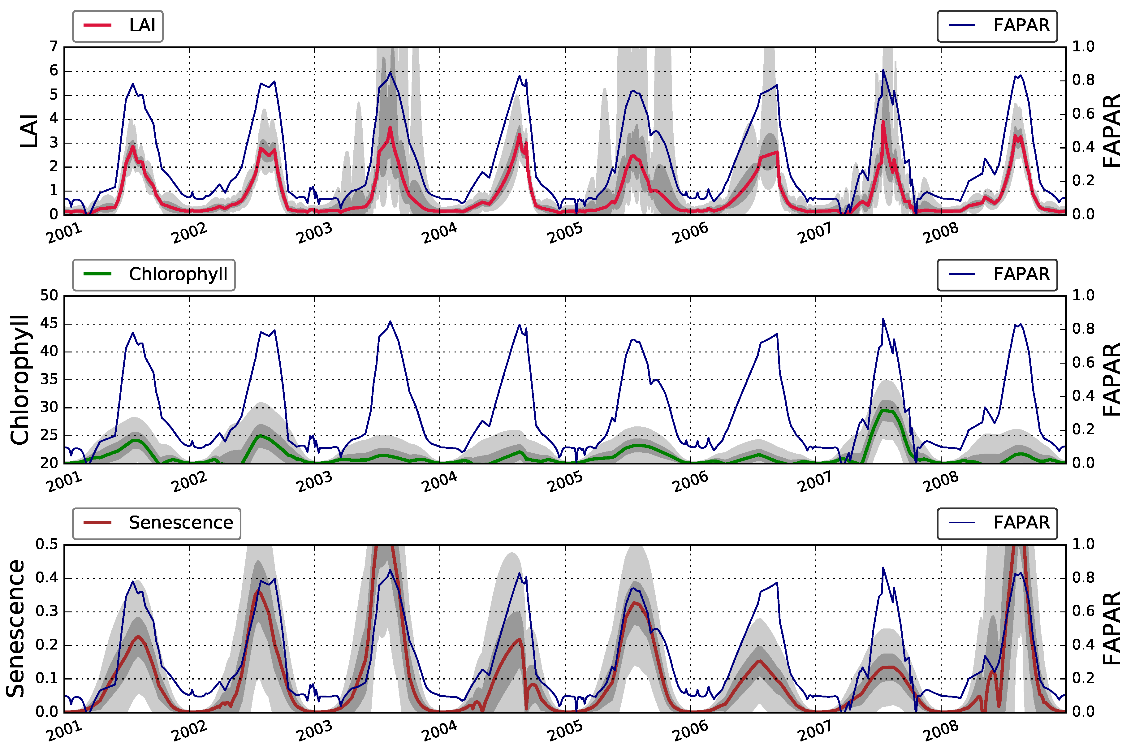
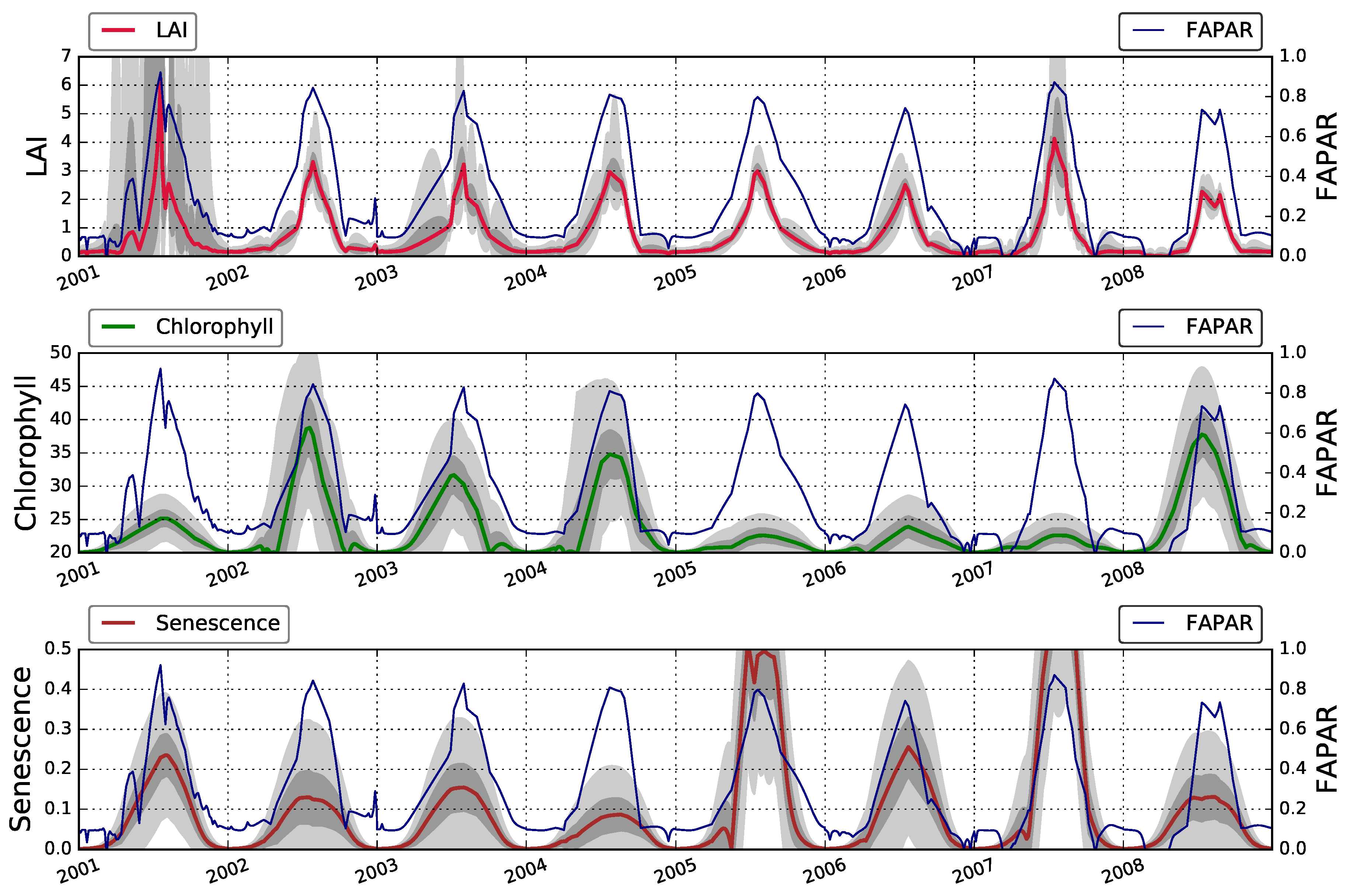
Figure 3, Figure 4 and Figure 5 show the evolution of LAI, leaf chlorophyll content, proportion of senescent material and FAPAR retrieved by EO-LDAS over the US-Ne1, US-Ne2 and US-Ne3 sites, respectively, between 2001 and 2008.

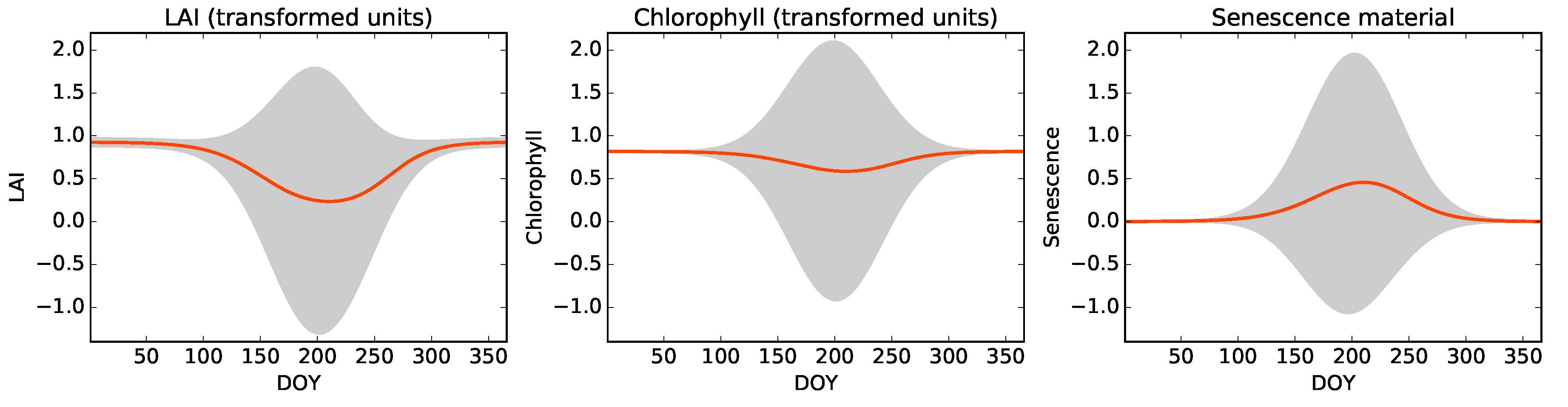
Figure 3 shows that the temporal trajectories of LAI, FAPAR, leaf chlorophyll content and the fraction of senescent leaves all broadly follow an annual pattern, with peaks in the summer months (around July-September). For LAI, the growing season is characterised by high uncertainties, a consequence of the saturation of reflectance for high LAI values and the small contribution of the prior term in this period (characterised by a large uncertainty). The temporal trajectories of the leaf pigments (chlorophyll and senescence) are characterised by large uncertainties, but the posterior mean shows a clear annual cycle, with chlorophyll leading senescence, as expected. This is a significant observation, as the temporal dynamics are not fixed by the prior term (the same functional form is used for all three parameters). The value of the proportion of senescent material does not go above 0.1, whereas at the end of the growing cycle one would expect there to be no senescent leaves. Large uncertainties in the parameters are due to complex interactions in how the parameters interact (with LAI and optical properties compensating each other). 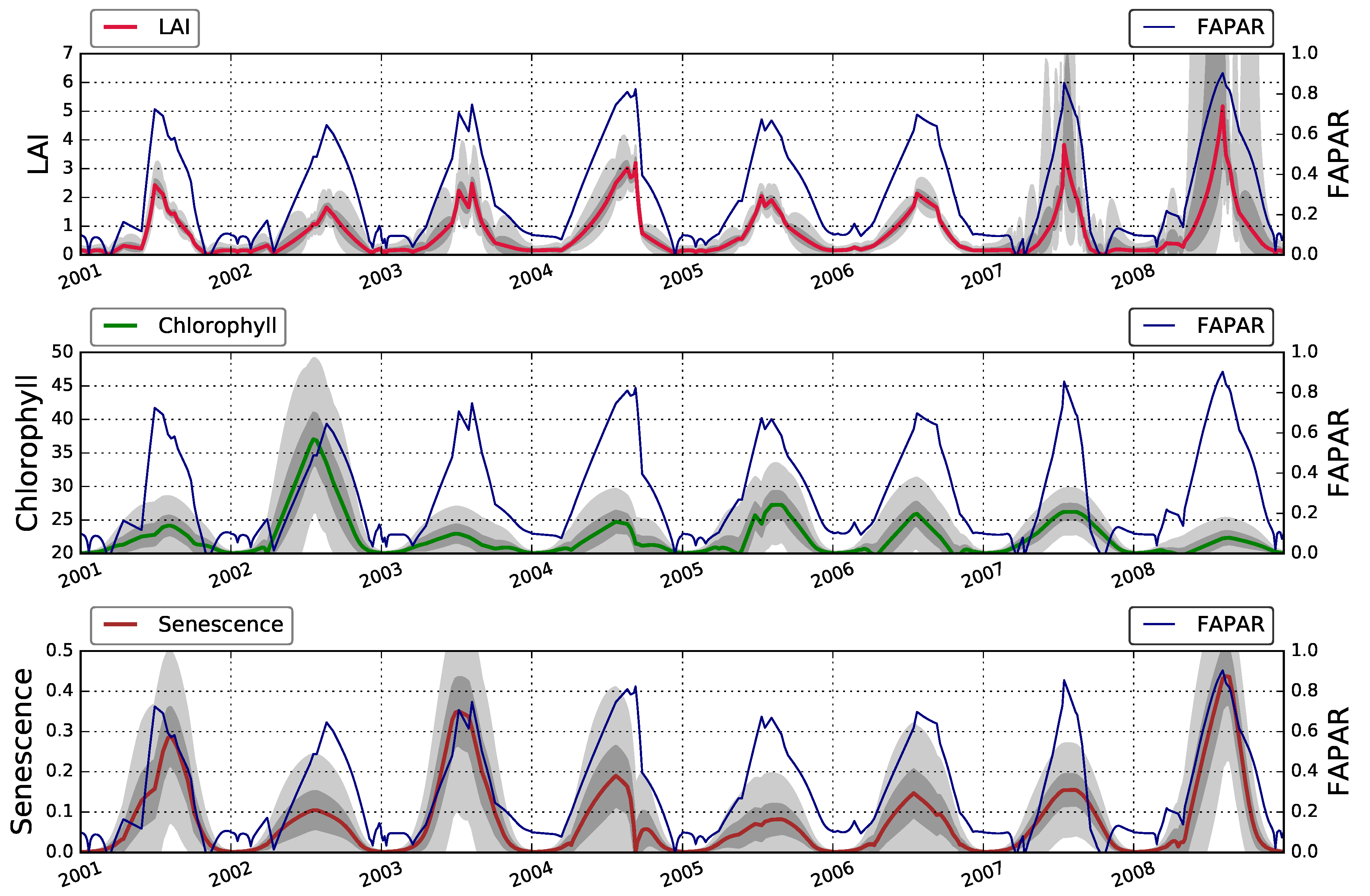It is important to note that the dynamic model used in the eoldas_ng inversion results in temporal continuous inferences, even though no observations might be available on a particular date. The results from the other two fields (Figure 4 and Figure 5) show a very similar behaviour, with both sites showing clear seasonalities for all retrieved parameters.

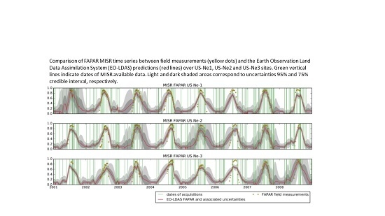
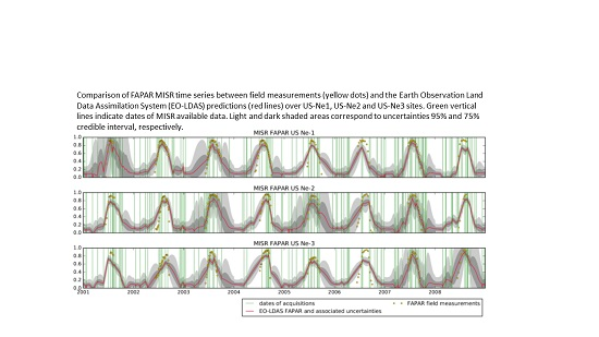
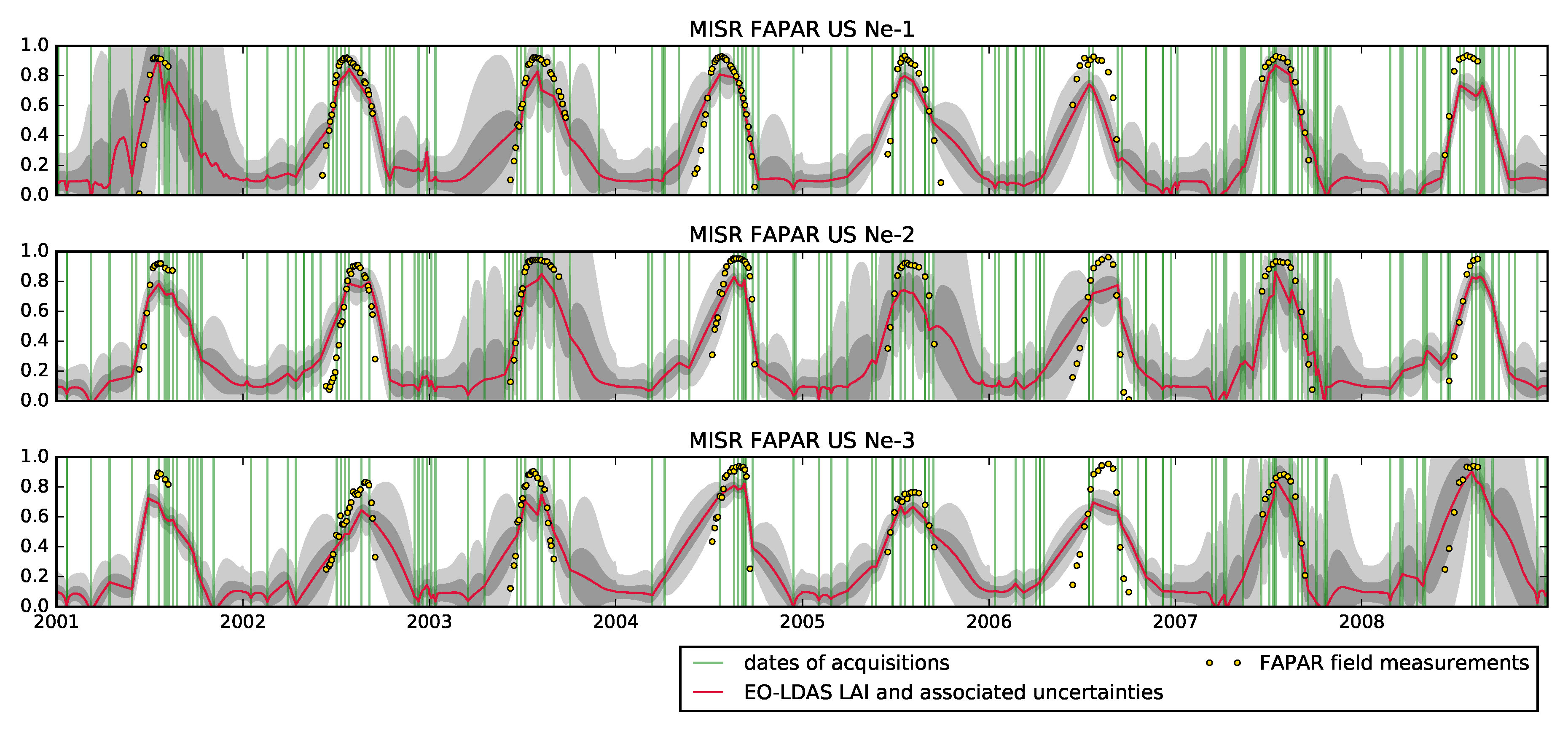
The parameters retrieved and shown in Figure 3 were then combined with the parameters in Table 2 and used to run the semi-discrete model and predict FAPAR. The MISR time series of EO-LDAS derived FAPAR are compared to ground-based measurements over US-Ne1, US-Ne2 and US-Ne3 sites (see Figure 6). The retrieved FAPAR tends to track the ground observations, with most of the ground observations being within the uncertainty bounds during the peak vegetation period. The inferences tend to overestimate the start and end of the growing season, and to slightly underestimate at peak LAI. The reason for the underestimate at the start of the growing season is that there is a paucity of observations at this time, and the retrieval is governed by the dynamic model interpolating between the observation-rich high LAI period and the prior-driven period with no vegetation at the beginning of the year. Towards the end of the growing season, the dynamic model sometimes fails to track the fast changes in FAPAR, again due to poor observation availability. Uncertainties are much larger when observations are not available and dynamic model restores the data. This is especially noticeable when temporal gaps are larger than one month. For example at the beginning and end of year 2002 (Ne-1), beginning of year 2003 (Ne-1), end of year 2004 (Ne-3), etc. 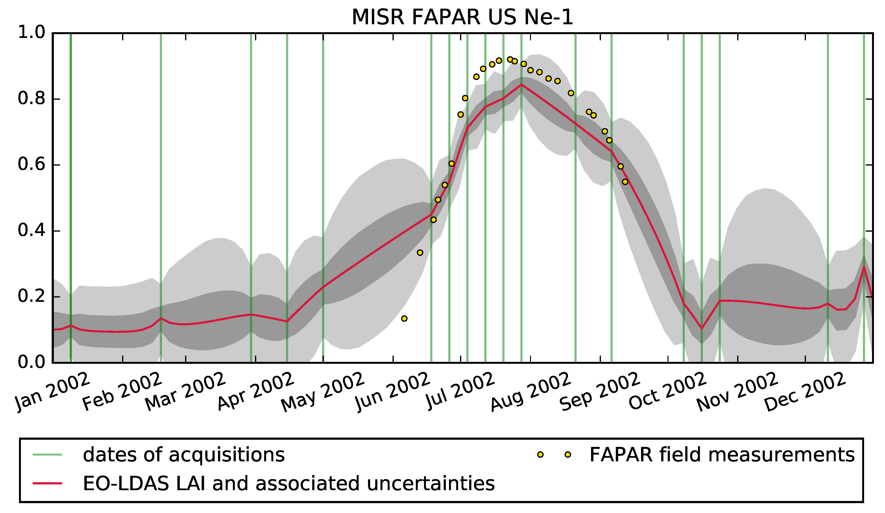In Figure 7 we show the retrieved FAPAR, uncertainties as well as ground measurements for US-Ne1 for 2002 only. It is clear that there are no observations available between the beginning of May and mid-July, and so the regularisation results in an overestimation over that period. Note, however, that the paucity of observations results in a noticeable increase in uncertainty, which results in the ground measurements actually being within the 95% credible interval.

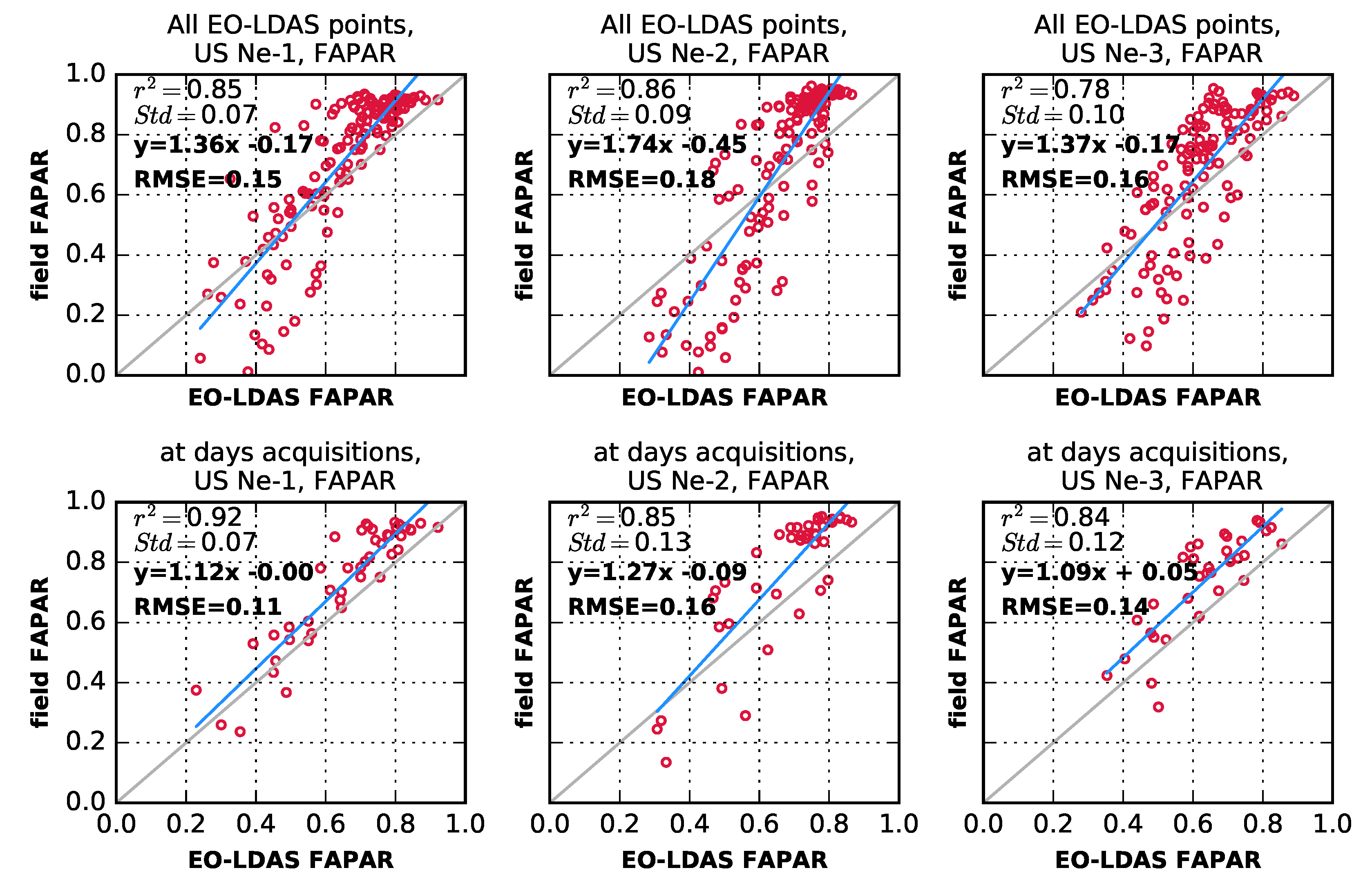
Figure 8 shows linear correlations between the retrieved FAPAR and the ground measurements for the three fields and all days for which ground measurements are available (top row) and also only for the dates where there are ground observations and coincident MISR overpasses (bottom row). It is clear from the top row in Figure 8 that the retrievals for low FAPAR are overestimated, and that this is caused by the interpolation provided by the dynamic model. When only points with observations are considered, the correlation increases, and the bias, slope and intercept all decrease, suggesting that the inversion works well where observations are available and the quality of the inferences drops as one moves away from the observations, with the dynamic model being too simple to track the changes in the rates of the process (as shown in Figure 7. In summary, we see that the correlation between retrieved and in situ FAPAR is high ($r^2>0.8$ for all dates, increasing to $r^2>0.85$ for retrievals coincidental with ground measurements) and the average $RMSE$ is 0.14 (only at days of satellite acquisitions). The slope of the retrieved FAPAR is consistent with an overestimation of FAPAR at the start and end of the growing season, and a slight underestimate in summer. When MISR observations are coincident with ground measurements, the slope becomes closer to the 1:1 line and the bias in the linear model tends to vanish.

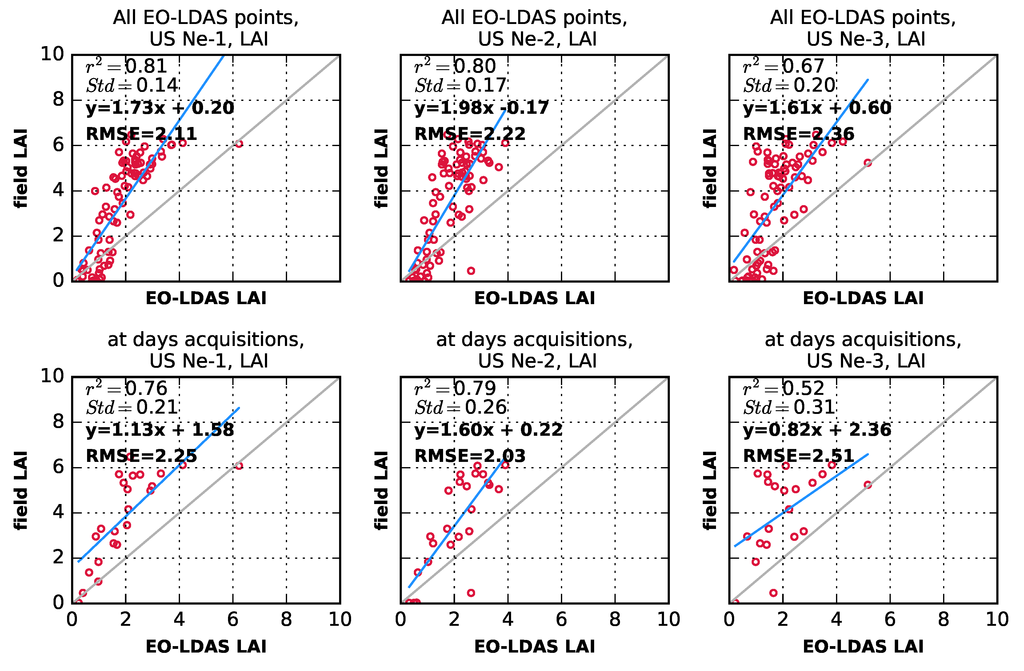
In Figure 9, we show the results of comparing ground-measured and retrieved LAI. The comparisons show that there is a strong correlation between retrieved and in situ LAI, but an important underestimation. One has to recall that any retrieval LAI from space or ground-based data correspond to an effective value which depends on the RT used during the retrieval or protocol in the case of in situ [68]. In general, retrieved effective LAI is close to the in situ measurements when LAI is low (≤2). After that, the retrieved LAI is lower than the in situ measurements. As the canopy becomes optically thicker, the sensitivity of the MISR observations decreases. This is expected as the value is close to the theoretical limit of retrieval of LAI as described in [69]. This is accompanied by an increase in uncertainty in the retrieved LAI estimate (see Figure 3). The summary statistics show that there is ample room for improvement: the correlations are 0.86, 0.80 and 0.68 (for US-Ne1, US-Ne2 and US-Ne3, respectively), slopes are 1.79, 1.86 and 1.55 (same order), and intercepts are −0.26, −0.36 and 0.28. $RMSE$ values are 1.92, 2.03 and 2.16.

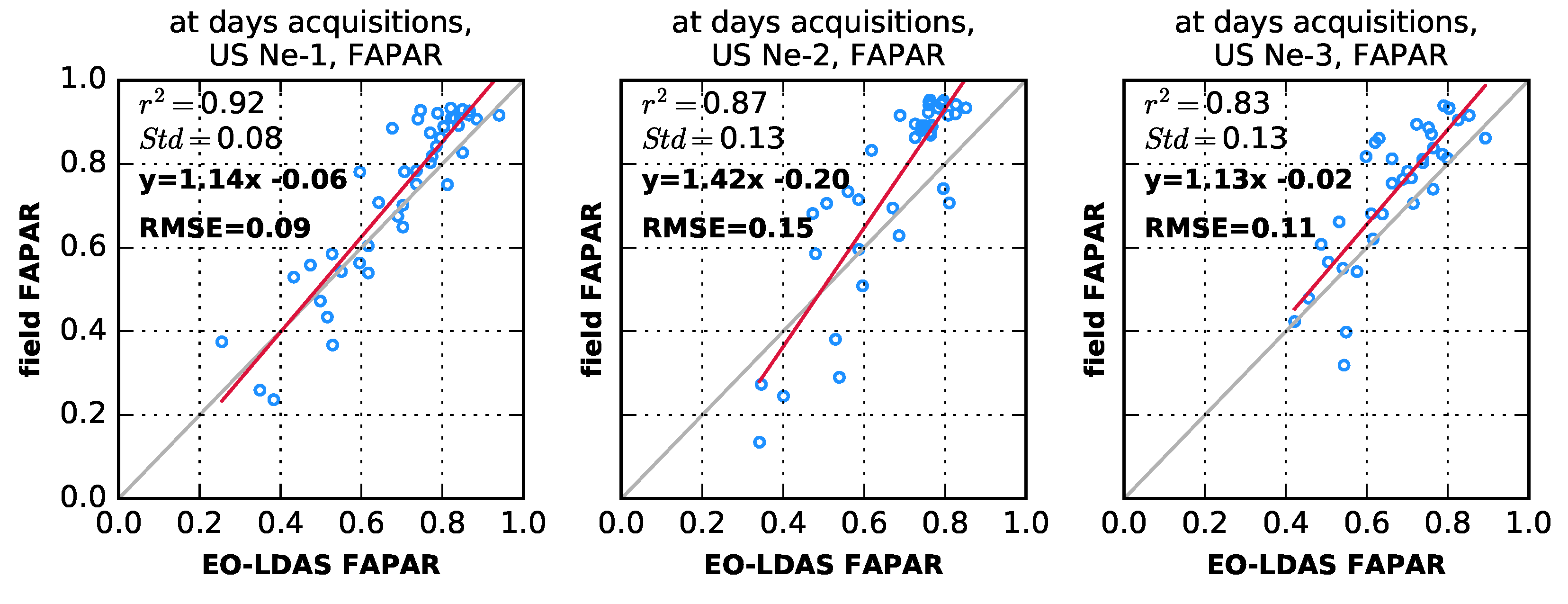
Although we have stated that the impact of the prior term should only be to tighten the retrieval in the period with no vegetation and few observations, this has not been demonstrated. In Figure 10, we show the comparison of retrieved FAPAR for the days of coincident satellite overpasses, where the prior is just set to a constant mean and uninformative (i.e., large) variance. The results are virtually the same as those shown in Figure 8, which demonstrates that the effect of the prior is minimal in the retrievals, as expected.

4.1. The JRC-TIP Results

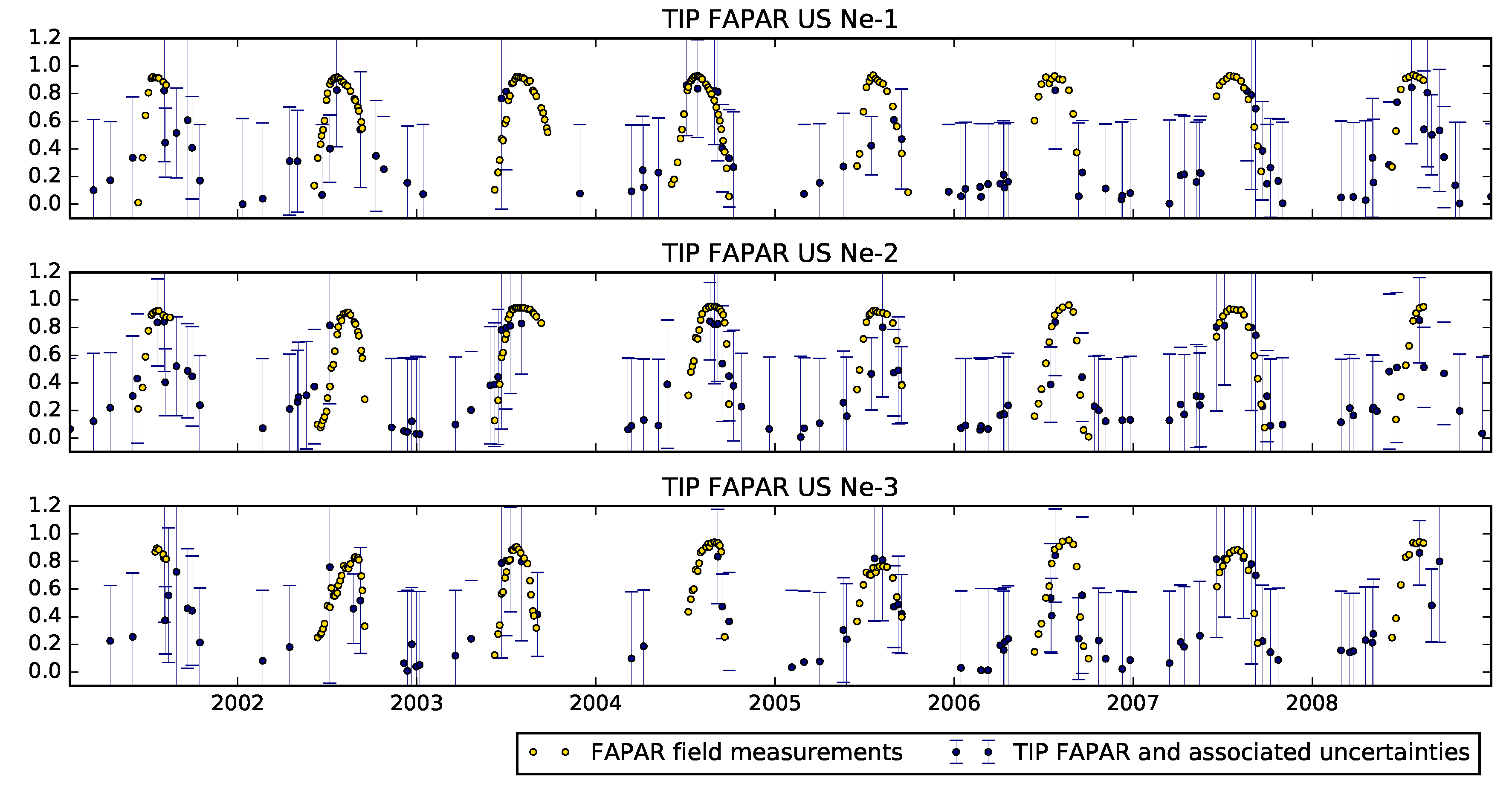
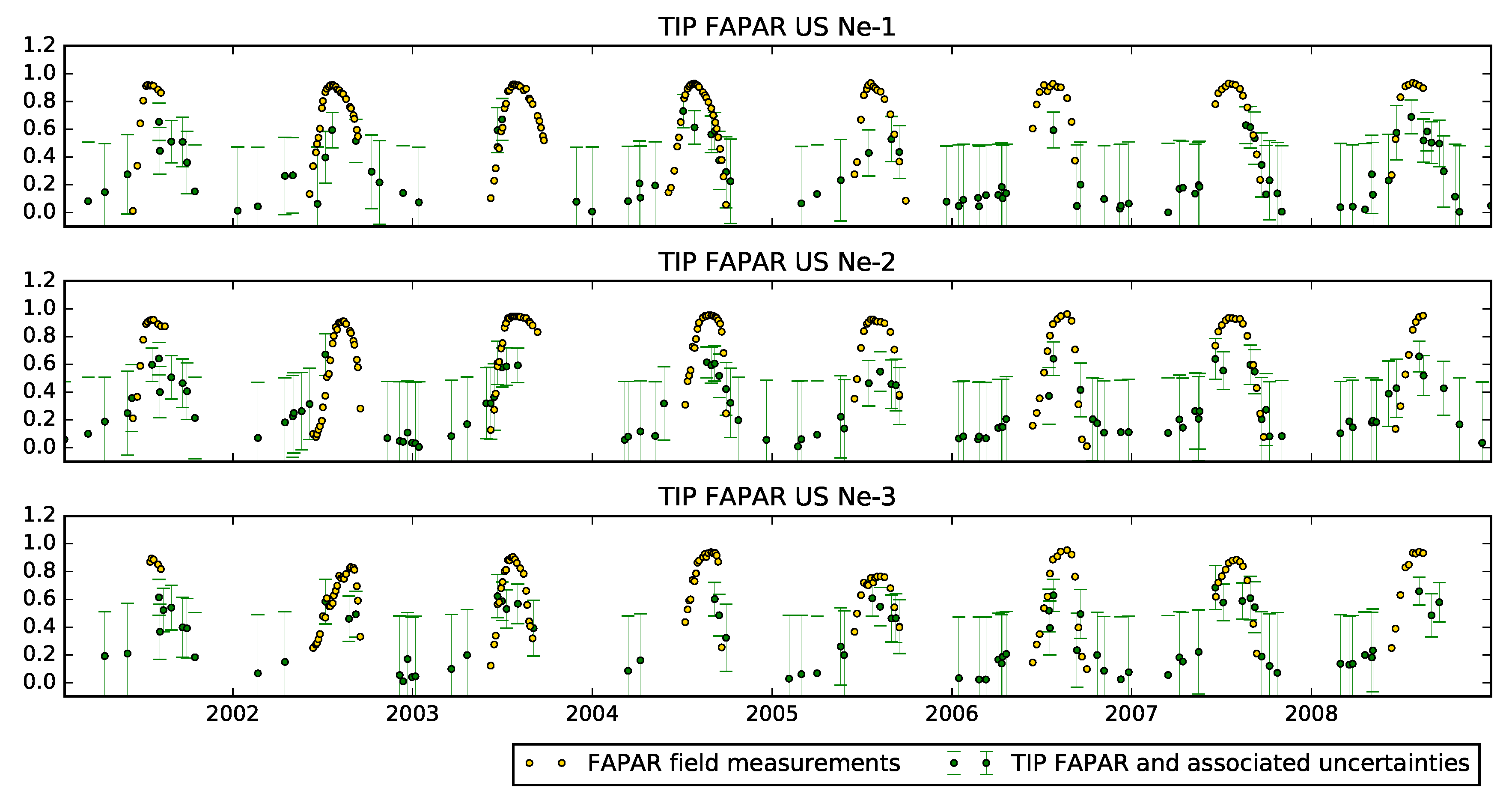
The results of FAPAR from the JRC-TIP product is shown in Figure 11. We note that this product is only able to provide an estimate of FAPAR when satellite observations are available. Furthermore, we note that for a number of years, the JRC-TIP FAPAR results in a more peaky growing season, which often peaks earlier than the ground measurements.

Figure 12 shows the results from the JRC-TIP product assuming green leaves (in effect, a tighter prior on the leaf single scattering albedo). The results show a clear underestimate of FAPAR compared to the in situ measurements.

We have also carried out a comparison between ground LAI and retrieved LAI, but we know that the retrieved LAI is effective [34,70]. The RT model used in this retrieval has indeed been developed for climate modelling assimilation of space land products; therefore it is based on a two-stream theory and retrieval values from surface broadband albedo. In [34] is recalled the need for a correction of a structure factor at the pixel resolution associated with the heterogeneous nature of the canopy volume. In general, the correlation coefficient is low (0.21–0.64), and there is a large bias (>1.3), as well as a scatter of around 2. The large bias is due to the JRC-TIP saturating at around three, as explained in [17].

4.2. The JRC MERIS Product

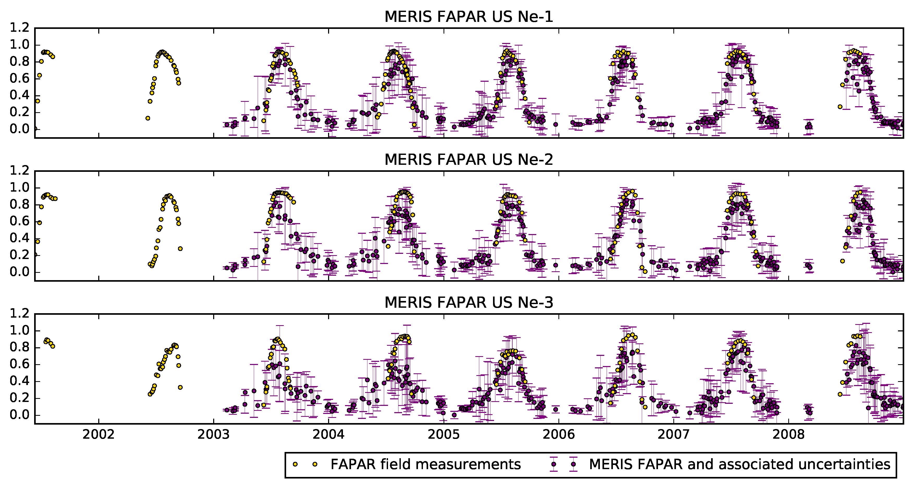
Figure 13 shows a comparison of the JRC MERIS FAPAR product and the in situ measurements. In general, the MERIS product provides an accurate description of the FAPAR annual trajectory, although with some underestimation of FAPAR at the peak of the growing season, as well as some overestimates of the very low FAPAR values at the beginning and end of the growing season.

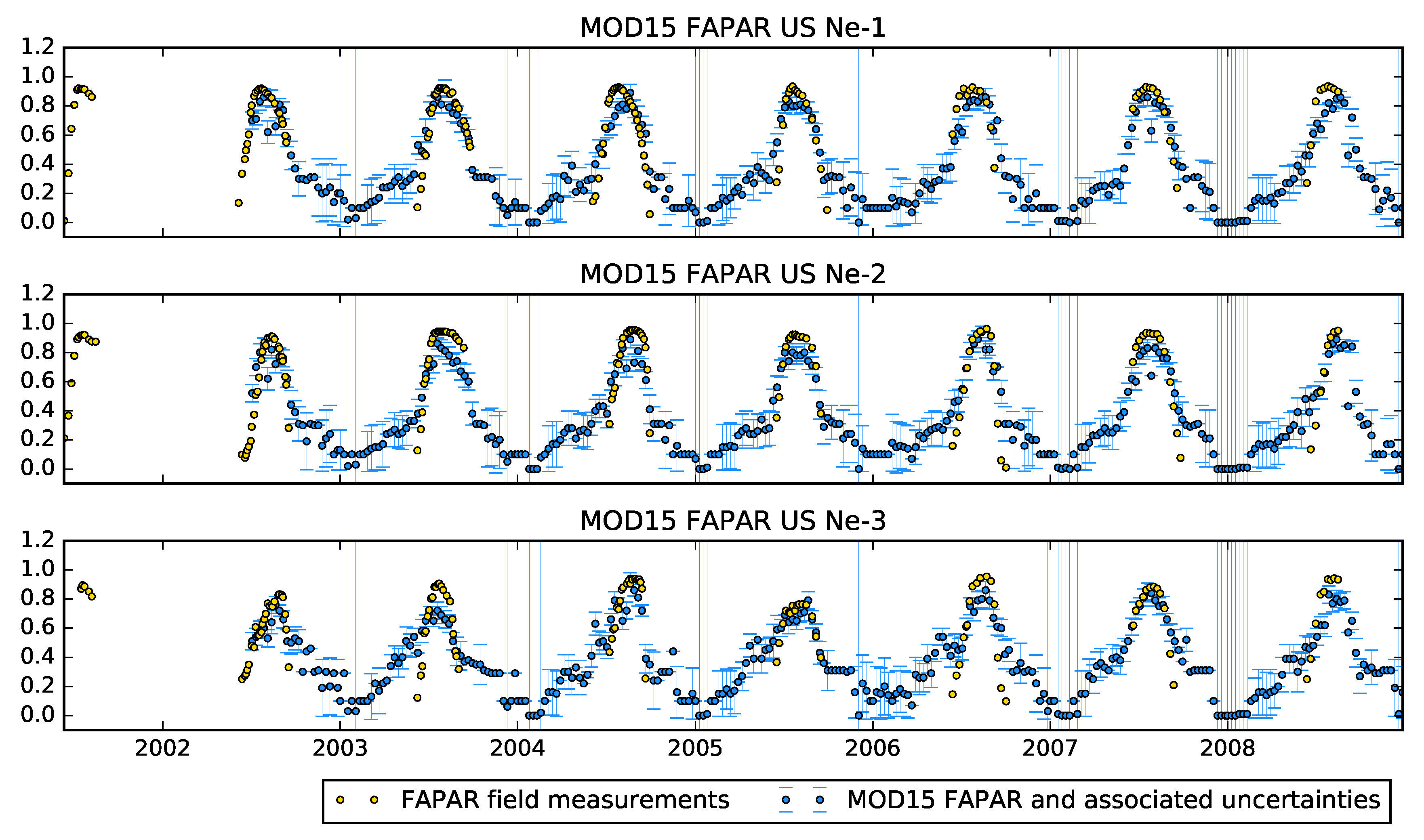
4.3. The MODIS FAPAR/LAI Product

Figure 14 shows FAPAR from the standard MODIS product MCD15A2H Collection 6. The results are generally good, the fine temporal sampling of using the two MODIS sensors resulting in a good coverage of the annual period. The estimates, however, tend to undershoot the peak FAPAR value consistently, and to overestimate the leading and trailing edges of the growing season.

The MODIS LAI product has a similar behaviour to the EO-LDAS LAI retrievals: with reasonably high correlations 0.84, 0.71 and 0.60 for US-Ne1, US-Ne2 and US-Ne3, respectively, but, again, resulting in an underestimate, particularly when the LAI is high.

5. Discussion

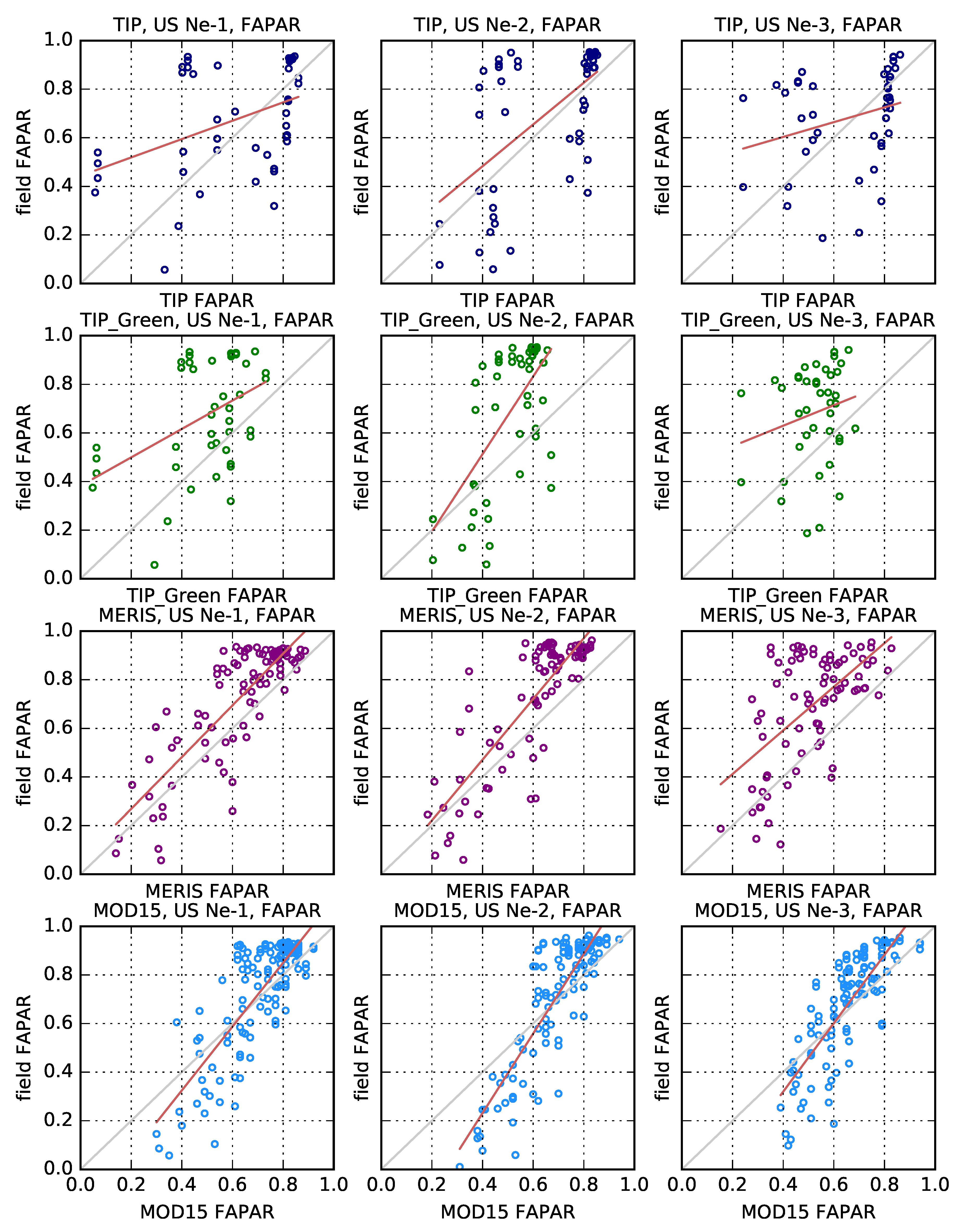
Comparisons of FAPAR retrievals for all products with ground-based data are shown in Figure 15 and

Table 3. Summary statistics derived from the comparison of FAPAR field measurements (2001–2008) collected on the US Ne-1 site with all corresponding EO-LDAS derived values (EO-LDAS all), EO-LDAS derived values at days of satellite acquisitions (EO-LDAS Obs.) and values obtained from JRC-TIP, JRC-TIP green, JRC MERIS and MODIS MCD15A2H products.

Stat. Param	EO-LDAS All	EO-LDAS Obs.	TIP	TIP Gr.	MERIS	MCD15
$r^2$	0.85	0.92	0.41	0.45	0.83	0.80
$\sigma$	0.07	0.07	0.13	0.18	0.08	0.09
$slope$	1.36	1.12	0.38	0.58	1.06	1.31
$intercept$	−0.17	−0.00	0.44	0.38	0.06	−0.20
$RMSE$	0.15	0.11	0.26	0.28	0.16	0.14

,

Table 4. Summary statistics derived from the comparison of FAPAR field measurements (2001–2008) collected on the US Ne-2 site with all corresponding EO-LDAS derived values (EO-LDAS all), EO-LDAS derived values at days of satellite acquisitions (EO-LDAS Obs.) and values obtained from JRC-TIP, JRC-TIP green, JRC MERIS and MODIS MCD15A2H products.

Stat. Param	EO-LDAS All	EO-LDAS Obs.	TIP	TIP Gr.	MERIS	MCD15
$r^2$	0.86	0.85	0.59	0.64	0.83	0.86
$\sigma$	0.09	0.13	0.17	0.27	0.09	0.09
$slope$	1.74	1.27	0.86	1.60	1.25	1.64
$intercept$	−0.45	−0.09	0.14	−0.13	−0.03	−0.42
$RMSE$	0.18	0.16	0.24	0.29	0.19	0.16

and

Table 5. Summary statistics derived from the comparison of FAPAR field measurements (2001–2008) collected on the US Ne-3 site with all corresponding EO-LDAS derived values (EO-LDAS all), EO-LDAS derived values at days of satellite acquisitions (EO-LDAS Obs.), and values obtained from JRC-TIP, JRC-TIP green, JRC MERIS and MODIS MCD15A2H products.

Stat. Param	EO-LDAS All	EO-LDAS Obs.	TIP	TIP Gr.	MERIS	MCD15
$r^2$	0.78	0.84	0.28	0.21	0.59	0.80
$\sigma$	0.10	0.12	0.17	0.31	0.14	0.10
$slope$	1.37	1.09	0.30	0.42	0.90	1.41
$intercept$	−0.17	0.05	0.48	0.46	0.23	−0.24
$RMSE$	0.16	0.14	0.23	0.26	0.26	0.14

. The EO-LDAS results have the highest linear correlation among all the compared products, as well as the lowest root mean square error. There is a positive slope, in line with the comments made in the last section about underestimates of FAPAR during the start and end of the vegetation period. If only dates where MISR observations are available are taken into account (remember that of all these products, EO-LDAS is the only one that will produce estimates for the entire time series), then the correlation increases, the slope approaches unity, and the bias disappears. These are remarkable results since MISR has far fewer observations per year (around 18) than MODIS (around 200) or MERIS (around 50), and yet the retrieved EO-LDAS MISR FAPAR performance is better than the other products (

Table 6. Average number of observations over all available years.

Field	MISR	MODIS	MERIS
US-Ne1	$16\pm 4$	$207\pm 37$	$50\pm 9$
US-Ne2	$18\pm 3$	$203\pm 34$	$50\pm 9$
US-Ne3	$14\pm 3$	$122\pm 18$	$51\pm 10$
Years	2001–2008	2001–2008	2003–2008

). The small number of observations and the very different temporal sampling of the MISR data affect the values of the regularisation parameter $\gamma$ retrieved by cross validation. In years with sparse observations, this can affect the impact of the dynamic model on the retrieved parameter trajectories. For example for US Ne-1, in 2001 (Figure 6), the regularisation parameter was found to be 3.6, in contrast to regularisation values around two orders of magnitude higher. This means that the character of the solution is likely to be less smooth and have higher associated uncertainties [48].

The poorest results in this comparison are with the JRC-TIP with green leaves, followed closely by the JRC-TIP with polychromatic leaves. The MERIS and MODIS products are comparable, with MERIS showing a slight negative bias. In general, all the tested products struggle to reach the highest in situ measured FAPAR, with a significant underestimate of FAPAR when in situ FAPAR is over 0.8. For EO-LDAS, this limitation can be traced back to the inability of the system to reach high values of LAI, a problem which is also expected with the JRC-TIP, where LAI is basically unconstrained whereas the optical properties of the leaves and soil are heavily constrained by priors. The other common striking feature of the comparisons is how the retrievals result in an overestimation of FAPAR when the in situ FAPAR is low (less than 0.3). This is a common feature of all products, but it is perhaps more exaggerated with the MODIS observations, which produce an overestimation of FAPAR where in situ values are below 0.6. In the case of the EO-LDAS retrievals, the effect is quite strong when all the in situ observations are considered, but the effect is attenuated when only the dates that have coincident observations are considered. By referring back to Figure 6, we explain this behaviour by pointing out that the low FAPAR values are usually in periods of very sparse MISR data (this is common to all years/sites), so that the effect is that of the system interpolating between two widely separated observations.

An important feature of the EO-LDAS approach is the use of a dynamic model for the retrievals. As the uncertainty in the dynamic model ($\gamma$ in Equation (14)) is constant, the trajectory of the state will tend to change not as rapidly as the observations on the ground, and this can lead to solutions that are too smooth in periods where the dynamics of the state are very fast. In our EO-LDAS results, the regularisation results in an increase in uncertainty, that although the MAP estimate overshoots the ground measurements, most of the measurements are within the uncertainty boundaries (except for a couple of cases of the earliest and latest stage of the growing season). Having more observations over those highly dynamic periods would alleviate this problem. In observation-sparse periods (e.g., 2001 for LAI in US-Ne1, Figure 3), observations produce a discontinuity in parameter trajectories, which is noticeable in the MAP solution, but small in terms of the total uncertainty. This artefact could be caused by locally defective convergence of the optimisation. In the case of abrupt changes, different techniques would need to be used, such as those presented in [71].

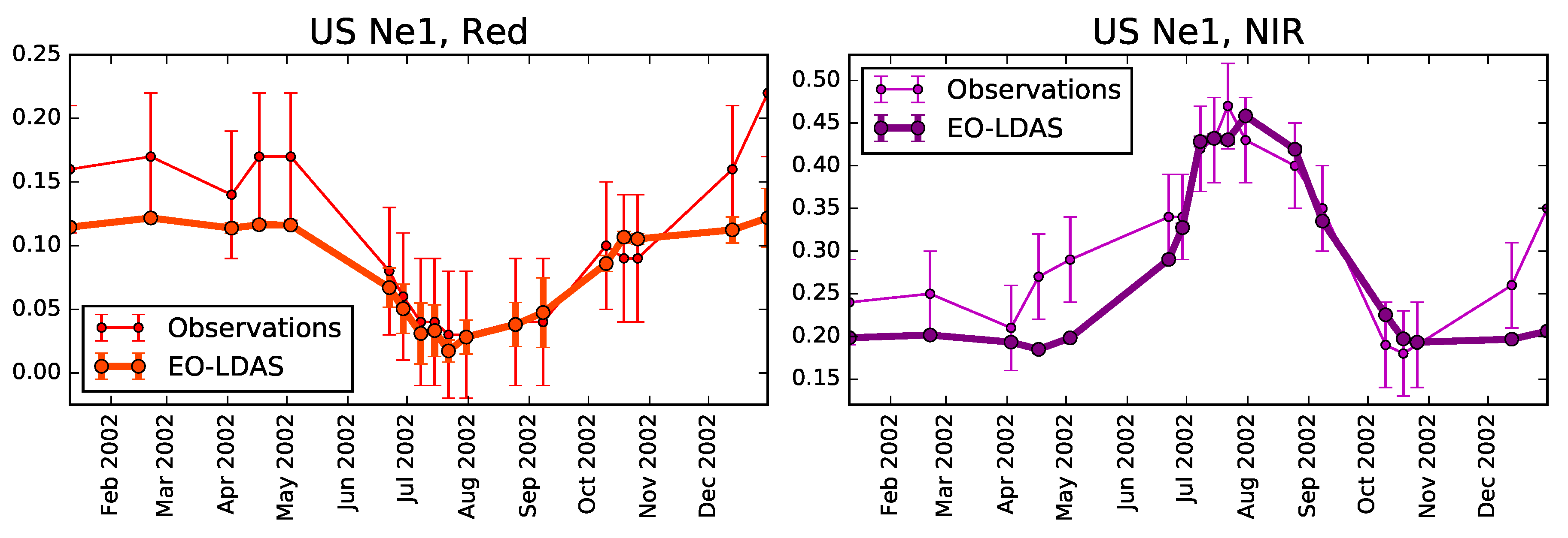
A further observation is that in the case at hand, we are using surface directional reflectance. The non-vegetative period is characterised by a rough soil surface with crop residue. The simple soil model is unable to properly model this period, for example being unable to, model BRDF effects present in the observations. The only freedom allowed by the model in this period is to modify canopy parameters to account for this, which is what causes the departure from zero of LAI in Figure 3 and the oscillations of $C_{ab}$ in the non-vegetative period. We can demonstrate this by running the following experiment: by fixing the leaf optical properties to sensible values and setting the LAI to be the (temporally interpolated) in situ LAI, we can then predict the observations. We can see the predictions and observations in the red and near-infra-red bands for 2002 and the US-Ne1 site in Figure 16. It is clear that the model fits the growing season reasonably well, but struggles with the bare soil period, indicating that here the RT model has problems replicating the data. Extending the RT model to have proper treatment of BRDF (for example, adding a Walthall [72] or Hapke [73,74] soil model) would alleviate this problem. Another approach would be to consider in the uncertainty budget in Equation (7) the model uncertainty. Under the assumption that the model uncertainty is (i) independent of the measurement uncertainty and (ii) normally distributed, we have that the observational constraint is given by:

$$J_{obs}\left(\overrightarrow{x}\right)=-\frac{1}{2}{(\overrightarrow{R}-H\left(\overrightarrow{x}\right))}^{\top }\left[{\mathbf{C}}_o^{-1}+{\mathbf{C}}_m^{-1}\right](\overrightarrow{R}-H\left(\overrightarrow{x}\right)),$$

(15)

a case that is readily implemented in eoldas_ng, but where the model uncertainty encoded in ${\mathbf{C}}_m$ might not be straightforward to assess. The effect of the prior introduced in this study goes somewhat to soften this problem, but leads to a dampening the contribution of $J_{obs}\left(\overrightarrow{x}\right)$ to the minimisation.

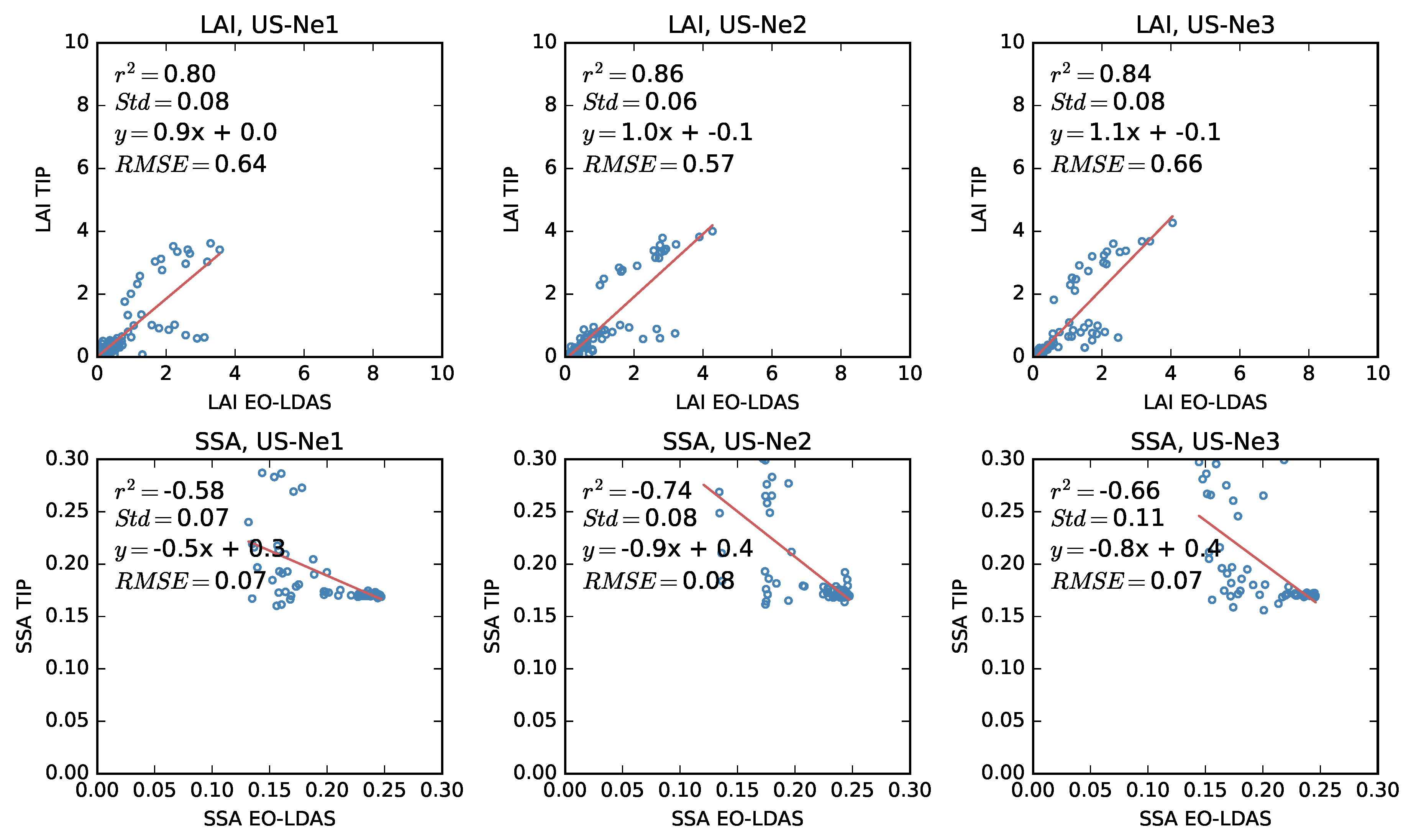
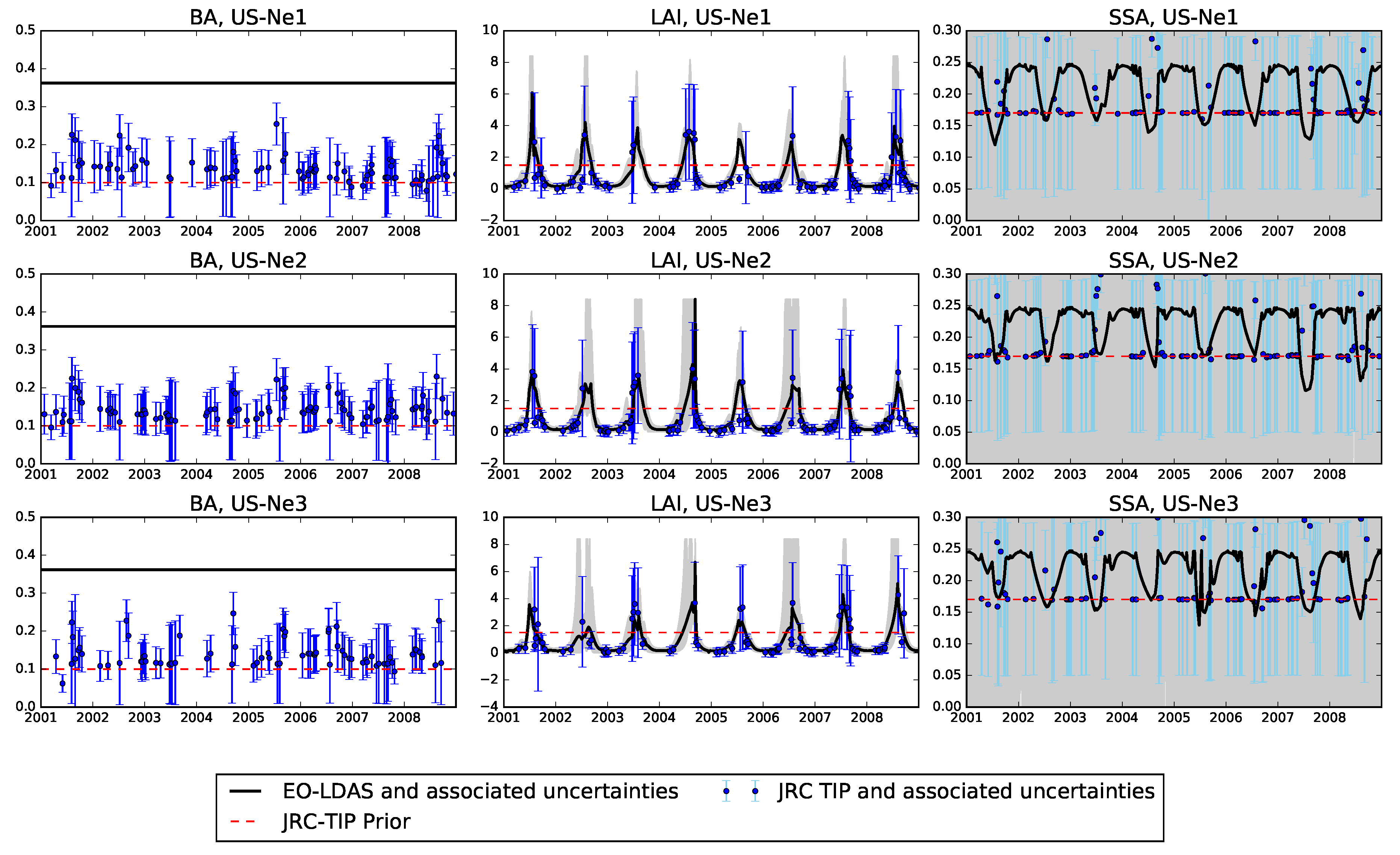
It is instructive to compare retrievals from the JRC-TIP product and EO-LDAS. Both approaches share the philosophy of calculating FAPAR by running a RT model with a parametrisation of the land surface state derived from inverting observations. In Figure 17, it is clear that there is a strong correlation between the LAI value retrieved from both approaches (taking into account that the retrieved effective LAI), but it is also apparent that the Single Scattering Albedo (SSA) estimates from both approaches is anti-correlated. In Figure 18, we can see that the JRC-TIP estimation for the soil background albedo in the visible changes throughout the year, whereas in the EO-LDAS case we have just fixed a particular soil spectral model. LAI (middle panel in Figure 18) shows some agreement, with EO-LDAS providing a more realistic trajectory due to the interpolation. The uncertainties from both products have similar trends with low values when LAI is low and high values in summer. The temporal evolution of the SSA in interesting: the JRC-TIP solution barely shifts from the prior, whereas the EO-LDAS version has a clear seasonality as a consequence of leaf chlorophyll content and fraction of senescent leaves changing throughout the growing period. In this case, the use of spectrally-resolved observations results in a richer interpretation of the EO data, rather than working from an spectrally integrated broad band, as is the case with the inputs to the JRC-TIP product.

The relatively good performance of the MERIS FAPAR algorithm is probably caused by its simplicity. Rather than targeting inference of a full set of land surface parameters, an equation is used to map from top of atmosphere reflectance to FAPAR, making strong assumptions on leaf single scattering albedo and soil background. Going through the EO-LDAS or JRC-TIP approaches needs the inference of a larger set of parameters, which necessarily results in larger uncertainties. However, a limitation of the MERIS algorithm is that it only produces an estimation where observations are present, and would need to be extended to cover different sensors simultaneously to produce a consistent FAPAR value. The method also does not estimate the underlying land surface parameters (e.g., LAI) which, if required for a particular application, would need to be obtained from a different product, potentially introducing inconsistencies e.g., due to different choices in the underlying RT model used for inversion.

The results from comparing the products that provide LAI estimates with ground LAI measurements show a common trend: all products underestimate LAI substantially. For the JRC-TIP, we note that this is expected as the LAI is effective [34], so this is not an entirely fair comparison. For the EO-LDAS MISR and MODIS products, we see an important underestimate of LAI when the ground value is high and effective LAI reach the saturation limits.. The different spatial scales of the satellite and ground measurements can result in very different LAI values [70,75,76]. It is interesting to note that the uncertainties in the retrieval of LAI with EO-LDAS MISR show a strong asymmetry (e.g., the uncertainty region above the posterior mean is much larger than the uncertainty region below the posterior mean) for high LAI (see Figure 3 and Figure 4), which is a statement of the limited sensitivity of the observations to high LAI.

6. Concluding Remarks

The main focus of this study is the estimation of daily FAPAR values by using EO-LDAS on MISR data. The evaluation of results against JRC-TIP, MERIS FR, MODIS MCD15 and in situ measured `green’ FAPAR was carried out for single pixels covering three agricultural FLUXNET sites over eight years. We have compared results from a number of different approaches and sensors: the EO-LDAS and JRC-TIP approaches both use MISR data (surface directional reflectance for the former and broadbands bi-hemispherical reflectance for the latter). These two methods rely on the inversion of an RT model, auxiliated by prior parameter distributions, and in the case of EO-LDAS, a dynamic regularisation model that allows the inference even at times where no satellite observations are present. The JRC MERIS FAPAR product uses MERIS top of the atmosphere reflectance and a polynomial that maps these measurements to FAPAR, and the MODIS product uses a Lookup Table (LUT) that maps red and near-infrared surface reflectance to FAPAR. It is important to point out that the difference in temporal sampling between the three instruments: MISR has a much lower number of observations than MERIS, and MERIS has a much lower number of observations than MODIS.

We have compared the different products with in situ ground measurements, and these indicate that FAPAR is retrieved with reasonable accuracy for three products: EO-LDAS ($r^2>0.8$, $RMSE<0.18$ in units of FAPAR), MERIS ($r^2>0.6$, $RMSE<0.2$) and MODIS ($r^2>0.8$, $RMSE<0.16$). The JRC-TIP results show a poor performance, with $r^2$ values between 0.3 and 0.6 and $RMSE$ in excess of 0.26. If only dates with MISR overpasses are considered for EO-LDAS, the estimates from EO-LDAS improve to an $r^2$ between 0.85 and 0.94, an $RMSE<0.14$ and with a bias that is between 2 and 7%.

All products have problems tracking the high FAPAR peak of the growing season, resulting in all products underestimating FAPAR at this point by 10–20%. Additionally, all products tend to overestimate FAPAR for the flanks of the growing season.

Three products (EO-LDAS, JRC-TIP and MODIS) also retrieve LAI (or effective LAI). The results all indicate that high LAI is underestimated. We propose that two processes are having an effect here: first, as the canopy becomes optically thicker, underestimation of LAI is expected [17], and secondly, the comparison of coarse resolution observations with point measurements introduces the effects of sub-pixel landscape heterogeneity [75,76]. In the literature [77,78], the use of empirical methods that have been trained with ground observations of the same area limits the generality of the methods for global applications. Additionally, no simultaneous inferences on FAPAR are presented in either of these two references. For the three coarse-resolution products that we considered in this study, comparisons with in situ LAI result in ($r^2>0.7$, $RMSE<2.2$) for EO-LDAS, ($r^2>0.6,RMSE<2.4$) for MODIS and $r^2$ between 0.4 and 0.6, $RMSE<2.3$ for the JRC-TIP (but again, note that LAI for the JRC-TIP is effective). The RMSE between all products and the ground observations is of the order of two units of LAI. In this study, we have used point measurements of LAI as a comparison. The recommended best practice is to use these measurements to provide a spatially explicit map, i.e., the minimum size of a validation site has to be compatible with resolution of satellite data [79,80].

Additionally, the MISR EO-LDAS approach also estimates the daily evolution of leaf chlorophyll content and fraction of senescent leaves. Both of these parameters show a credible temporal trajectory (although they have not been compared with any in situ measurements), with a clear arch for both when LAI is high, but showing leaf chlorophyll dropping off earlier than senescence and senescence growing later than leaf chlorophyll. This is a very encouraging result, as no timing information on these two parameters as provided in the priors pdf used, and only observations from four spectral bands in the visible-NIR region were available.

The MISR EO-LDAS approach is characterised by large uncertainties in both land surface parameters (LAI, $C_{ab}$, $C_{brown}$), as well as fluxes (FAPAR). This is inevitable due to the poor temporal sampling. We note that high uncertainty in LAI during periods of high LAI is to be expected, and we note that this uncertainty (see Figure 3) is asymmetric: high above the MAP estimate and low below, encoding the inability of the RT model of interpreting the reflectance as a clear high value of LAI, but quite certain that it is larger than e.g., two. This is in marked contrast to the uncertainties in LAI for the JRC-TIP product (see Figure 18). The advantage of EO-LDAS is obtained by using the quasi-linearising transformations in Table 2.

In this paper, we deliberately only compare EO-derived estimates of FAPAR from approaches that rely on the inversion of RT models (and hence, ought to show some level of consistency and physical accuracy). However, we also note that there is a long history of exploiting the relationship between empirical vegetation indices (such as NDVI) and FAPAR. Recent work by [22] has used ground spectral measurements, as well as MODIS 250-m NDVI data to revisit these relationships for the sites that are considered in this study. In [22], different regressions relating NDVI to FAPAR are shown to produce a very large spread of possible values of FAPAR. The authors also derive a set of equations that can be applied to the site, but note that they need to be split by crop type (maize and soya) and by development (vegetative and reproductive) stage. The resulting correlations are similar to those reported in the present study, whereas other non-specific formulations of the mapping between NDVI and FAPAR show a large scatter, indicating that significant effort is required for local calibration to provide useful results. In [22], additional understanding of the crop type and phenology are required for optimal performance. Using the EO-LDAS approach, we have only used very generic priors detailing vegetation structure and leaf optical properties, although of course, more informative priors could be used, if they were available. As part of the process, estimates of widely-used land surface parameters have also been retrieved, along with well-quantified uncertainty. This is a particular feature of the EO-LDAS approach, which provides an important benefit over other methods. In particular, LAI has been retrieved with an error that is in the range of other typical global LAI products for this site, and more generally [81]. The EO-LDAS approach also exploits temporal regularisation to provide a consistently gap-filled estimate of parameters even when no observations are available. The use of radiative transfer models within this regularisation framework allows for simple inclusion of observations from other sensors, as these are interpreted and assimilated in terms of common descriptions of the land surface. These are important advantages of the EO-LDAS approach presented here, and they have been proven to be useful: having a much poorer temporal sampling regime, results from the EO-LDAS MISR approach are in line with the JRC MERIS and MODIS FAPAR products. LAI retrievals are also in line with the other products, indicating that the approach based on interpretation of the observations using physical models succeeds in providing consistent estimates of FAPAR and other land surface parameters.

An additional important consideration is that the EO-LDAS retrieved parameters are self-consistent, i.e., the same physical (RT) model assumptions are made to retrieve e.g., both LAI and FAPAR. This is important if such parameter estimates are then used to drive models [8]. Inconsistencies across suites of parameters can result in hard-to-trace model deviations and uncertainties in model predictions. Parameter consistency is hard, if not impossible, to ensure when using locally-calibrated empirical relationships where different parts of the state vector (e.g., LAI, leaf chlorophyll concentration or FAPAR) are derived separately. Further, the incorporation of priors makes explicit the assumption that both the chosen physical model and sets of priors are adequate for the task at hand. The use of Bayesian approaches with physical models necessitates clear statements about observational uncertainty [82,83]. These ought to be provided as the standard with EO-derived surface reflectance products, but rarely are in practice due to the limitations of retrieval processes. Finally, although in this study we have ignored the uncertainty associated with using an RT model, this can be readily introduced in the EO-LDAS formalism, if information on the properties of this error were available. Unacknowledged model error can result in biases in the solution.

We demonstrate that at least for the particular sites shown here, EO-LDAS is able to estimate absorbed fluxes, other biophysical parameters and associated uncertainties relying on multi-angular surface reflectance observations. The EO-LDAS scheme also allows for a simple combination of other available observations, thus opening the door to multi-sensor estimates of fluxes and/or biophysical parameters. The estimation of uncertainties, as well as the retrieval of a complete set of ground biophysical parameters is also an important tool in providing data that allows us to learn more about the land surface.

References

1. Global Terrestrial Observing System (GTOS). Terrestrial Essential Climate Variables for Climate Change Assessment, Mitigation and Adaptation; Technical Report; Food and Agriculture Organization (FAO): Rome, Italy, 2008. [Google Scholar]
2. Gower, S.T.; Kucharik, C.J.; Norman, J.M. Direct and Indirect Estimation of Leaf Area Index, fAPAR, and Net Primary Production of Terrestrial Ecosystems. Remote Sens. Environ. 1999, 70, 29–51. [Google Scholar] [CrossRef]
3. Gobron, N.; Pinty, B.; Mélin, F.; Taberner, M.; Verstraete, M.M.; Belward, A.; Lavergne, T.; Widlowski, J. The state of vegetation in Europe following the 2003 drought. Int. J. Remote Sens. 2005, 26, 2013–2020. [Google Scholar] [CrossRef]
4. Senna, M.; Costa, M.; Shimabukuro, Y. Fraction of photosynthetically active radiation absorbed by Amazon tropical forest: A comparison of field measurements, modeling, and remote sensing. J. Geophys. Res. Biogeosci. 2005, 110, G01008. [Google Scholar] [CrossRef]
5. Verstraete, M.M.; Gobron, N.; Aussedat, O.; Robustelli, M.; Pinty, B.; Widlowski, J.L.; Taberner, M. An automatic procedure to identify key vegetation phenology events using the JRC-FAPAR products. Adv. Space Res. 2008, 41, 1773–1783. [Google Scholar] [CrossRef]
6. Coops, N.; Wulder, M.; Duro, D.; Han, T.; Berry, S. The development of a Canadian dynamic habitat index using multi-temporal satellite estimates of canopy light absorbance. Ecol. Indic. 2008, 8, 754–766. [Google Scholar] [CrossRef]
7. Kaminski, T.; Rayner, P.J.; Voßbeck, M.; Scholze, M.; Koffi, E. Observing the continental-scale carbon balance: Assessment of sampling complementarity and redundancy in a terrestrial assimilation system by means of quantitative network design. Atmos. Chem. Phys. 2012, 12, 7867–7879. [Google Scholar] [CrossRef]
8. Loew, A.; van Bodegom, P.M.; Widlowski, J.L.; Otto, J.; Quaife, T.; Pinty, B.; Raddatz, T. Do we (need to) care about canopy radiation schemes in DGVMs? Caveats and potential impacts. Biogeosciences 2014, 11, 1873–1897. [Google Scholar] [CrossRef]
9. Weiss, M.; Baret, F.; Garrigues, S.; Lacaze, R. LAI and fAPAR CYCLOPES global products derived from VEGETATION. Part 2: Validation and comparison with MODIS collection 4 products. Remote Sens. Environ. 2007, 110, 317–331. [Google Scholar] [CrossRef]
10. Román, M.O.; Schaaf, C.B.; Lewis, P.; Gao, F.; Anderson, G.P.; Privette, J.L.; Strahler, A.H.; Woodcock, C.E.; Barnsley, M. Assessing the coupling between surface albedo derived from MODIS and the fraction of diffuse skylight over spatially-characterized landscapes. Remote Sens. Environ. 2010, 114, 738–760. [Google Scholar] [CrossRef]
11. D’Odorico, P.; Gonsamo, A.; Pinty, B.; Gobron, N.; Coops, N.; Mendez, E.; Schaepman, M.E. Intercomparison of fraction of absorbed photosynthetically active radiation products derived from satellite data over Europe. Remote Sens. Environ. 2014, 142, 141–154. [Google Scholar] [CrossRef]
12. Global Climate Observing System (GCOS). The Second Report on the Adequacy of the Global Observing Systems for Climate in Support of the UNFCCC. Available online: https://www.wmo.int/pages/prog/gcos/Publications/gcos-822AR.pdf (accessed on 26 June 2017).
13. Kimes, D.; Knyazikhin, Y.; Privette, J.; Abuelgasim, A.; Gao, F. Inversion methods for physically based models. Remote Sens. Rev. 2000, 18, 381–439. [Google Scholar] [CrossRef]
14. Hadamard, J. Sur les problèmes aux dérivées partielles et leur signification physique. Princet. Univ. Bull. 1902, 13, 49–52. [Google Scholar]
15. Combal, B.; Baret, F.; Weiss, M.; Trubuil, A.; Mace, D.; Pragnere, A.; Myneni, R.; Knyazikhin, Y.; Wang, L. Retrieval of canopy biophysical variables from bidirectional reflectance using prior information to solve the ill-posed inverse problem. Remote Sens. Environ. 2002, 84, 1–15. [Google Scholar] [CrossRef]
16. Lewis, P.; Gómez-Dans, J.; Kaminski, T.; Settle, J.; Quaife, T.; Gobron, N.; Styles, J.; Berger, M. An Earth Observation Land Data Assimilation System (EO-LDAS). Remote Sens. Environ. 2012, 120, 219–235. [Google Scholar] [CrossRef]
17. Pinty, B.; Jung, M.; Kaminski, T.; Lavergne, T.; Mund, M.; Plummer, S.; Thomas, E.; Widlowski, J.L. Evaluation of the JRC-TIP 0.01° products over a mid-latitude deciduous forest site. Remote Sens. Environ. 2011, 115, 3567–3581. [Google Scholar] [CrossRef]
18. Kaminski, T.; Mathieu, P.P. Reviews and syntheses: Flying the satellite into your model: On the role of observation operators in constraining models of the Earth system and the carbon cycle. Biogeosciences 2017, 14, 2343–2357. [Google Scholar] [CrossRef]
19. Kaminski, T.; Pinty, B.; Voßbeck, M.; Lopatka, M.; Gobron, N.; Robustelli, M. Consistent retrieval of land surface radiation products from EO, including traceable uncertainty estimates. Biogeosciences 2017, 14, 2527–2541. [Google Scholar] [CrossRef]
20. Lewis, P.; Gomez-Dans, J.; Kaminski, T.; Settle, J.; Quaife, T.; Gobron, N.; Styles, J.; Berger, M. Data assimilation of Sentinel-2 observations: Preliminary results from EO-LDAS and outlook. In Proceedings of the First Sentinel-2 Preparatory Symposium, Frascati, Italy, 23–27 April 2012; Volume ESA SP-707. [Google Scholar]
21. Gómez-Dans, J.L.; Lewis, P.E.; Disney, M. Efficient Emulation of Radiative Transfer Codes Using Gaussian Processes and Application to Land Surface Parameter Inferences. Remote Sens. 2016, 8, 119. [Google Scholar]
22. Gitelson, A.A.; Peng, Y.; Huemmrich, K.F. Relationship between fraction of radiation absorbed by photosynthesizing maize and soybean canopies and NDVI from remotely sensed data taken at close range and from MODIS 250 m resolution data. Remote Sens. Environ. 2014, 147, 108–120. [Google Scholar] [CrossRef]
23. Myneni, R.; Knyazikhin, Y.; Park, T. MCD15A2H MODIS/Terra+Aqua Leaf Area Index/FPAR 8-day L4 Global 500 m SIN Grid V006. NASA EOSDIS Land Processes DAAC, 2015. Available online: https://doi.org/10.5067/MODIS/MCD15A2H.006 (acccessed on 26 June 2017).
24. Pinty, B.; Widlowski, J.L.; Gobron, N.; Verstraete, M.M.; Diner, D.J.; Member, A. Uniqueness of Multiangular Measurements—Part I: An Indicator of Subpixel Surface Heterogeneity From MISR. IEEE Trans. Geosci. Remote Sens. 2002, 40, 1560–1573. [Google Scholar] [CrossRef]
25. Deschamps, P.Y.; Breon, F.M.; Leroy, M.; Podaire, A.; Bricaud, A.; Buriez, J.C.; Seze, G. The POLDER mission: Instrument characteristics and scientific objectives. IEEE Trans. Geosci. Remote Sens. 1994, 32, 598–615. [Google Scholar] [CrossRef]
26. SLSTR Instrument. Available online: https://sentinel.esa.int/web/sentinel/technical-guides/sentinel-3-slstr/instrument/description (accessed on 20 June 2017).
27. Diner, D.J.; Beckert, J.C.; Reilly, T.H.; Bruegge, C.J.; Conel, J.E.; Kahn, R.A.; Martonchik, J.V.; Ackerman, T.P.; Davies, R.; Gerstl, S.A.W.; et al. Multi-angle Imaging SpectroRadiometer (MISR) instrument description and experiment overview. IEEE Trans. Geosci. Remote Sens. 1998, 36, 1072–1087. [Google Scholar] [CrossRef]
28. Knyazikhin, Y.; Martonchik, J.V.; Myneni, R.B.; Diner, D.J.; Running, S.W. Synergistic algorithm for estimating vegetation canopy leaf area index and fraction of absorbed photosynthetically active radiation from MODIS and MISR data. J. Geophys. Res. 1998, 103, 32257. [Google Scholar] [CrossRef]
29. Gobron, N.; Pinty, B.; Verstraete, M.M.; Martonchik, J.V.; Knyazikhin, Y.; Diner, D.J. Potential of multiangular spectral measurements to characterize land surfaces: Conceptual approach and exploratory application. J. Geophys. Res. 2000, 105, 17539. [Google Scholar] [CrossRef]
30. Widlowski, J.L.; Pinty, B.; Gobron, N.; Verstraete, M.M.; Diner, D.J.; Davis, A.B. Canopy structure parameters derived from multi-angular remote sensing data for terrestrial carbon studies. Clim. Chang. 2004, 67, 403–415. [Google Scholar] [CrossRef]
31. Laurent, V.C.; Verhoef, W.; Clevers, J.G.; Schaepman, M.E. Inversion of a coupled canopy-atmosphere model using multi-angular top-of-atmosphere radiance data: A forest case study. Remote Sens. Environ. 2011, 115, 2603–2612. [Google Scholar] [CrossRef]
32. Pinty, B.; Lavergne, T.; Voßbeck, M.; Kaminski, T.; Aussedat, O.; Giering, R.; Gobron, N.; Taberner, M.; Verstraete, M.M.; Widlowski, J.L. Retrieving surface parameters for climate models from Moderate Resolution Imaging Spectroradiometer (MODIS)-Multiangle Imaging Spectroradiometer (MISR) albedo products. J. Geophys. Res. 2007, 112, D10116. [Google Scholar] [CrossRef]
33. Verstraete, M.M.; Member, S.; Hunt, L.A.; Scholes, R.J.; Clerici, M.; Pinty, B.; Nelson, D.L. Generating 275-m Resolution Land Surface Products From the Multi-Angle Imaging SpectroRadiometer Data. IEEE Trans. Geosci. Remote Sens. 2012, 50, 3980–3990. [Google Scholar] [CrossRef]
34. Pinty, B.; Lavergne, T.; Dickinson, R.E.; Widlowski, J.L.; Gobron, N.; Verstraete, M.M. Simplifying the Interaction of Land Surfaces with Radiation for Relating Remote Sensing Products to Climate Models. J. Geophys. Res. Atmos. 2006, 111, D02116. [Google Scholar] [CrossRef]
35. Pinty, B.; Clerici, M.; Andredakis, I.; Kaminski, T.; Taberner, M.; Verstraete, M.M.; Gobron, N.; Plummer, S.; Widlowski, J.L. Exploiting the MODIS albedos with the Two-stream Inversion Package (JRC-TIP): 2. Fractions of transmitted and absorbed fluxes in the vegetation and soil layers. J. Geophys. Res. Atmos. 2011, 116, D09106. [Google Scholar] [CrossRef]
36. Viña, A.; Gitelson, A.A. New developments in the remote estimation of the fraction of absorbed photosynthetically active radiation in crops. Geophys. Res. Lett. 2005, 32, L17403. [Google Scholar]
37. MISR Web Site. Available online: http://www-misr.jpl.nasa.gov/ (accessed on 27 January 2017).
38. Giering, R.; Kaminski, T. Recipes for adjoint code construction. ACM Trans. Math. Softw. 1998, 24, 437–474. [Google Scholar] [CrossRef]
39. Gobron, N.; Pinty, B.; Verstraete, M.; Widlowski, J.L. Advanced vegetation indices optimized for up-coming sensors: Design, performance, and applications. IEEE Trans. Geosci. Remote Sens. 2000, 38, 2489–2505. [Google Scholar]
40. Gobron, N.; Pinty, B.; Verstraete, M.; Govaerts, Y. The MERIS Global Vegetation Index (MGVI): Description and preliminary application. Int. J. Remote Sens. 1999, 20, 1917–1927. [Google Scholar] [CrossRef]
41. Gobron, N.; Pinty, B.; Aussedat, O.; Taberner, M.; Faber, O.; Mélin, F.; Lavergne, T.; Robustelli, M.; Snoeij, P. Uncertainty estimates for the FAPAR operational products derived from MERIS—Impact of top-of-atmosphere radiance uncertainties and validation with field data. Remote Sens. Environ. 2008, 112, 1871–1883. [Google Scholar] [CrossRef]
42. Gobron, N. Uncertainties assessment for MERIS/OLCI FAPAR. In Proceedings of the 2015 ESA Sentinel-3 for Science Workshop, Venice, Italy, 2–5 June 2015. [Google Scholar]
43. Yang, W.; Tan, B.; Huang, D.; Rautiainen, M.; Shabanov, N.V.; Wang, Y.; Privette, J.L.; Huemmrich, K.F.; Fensholt, R.; Sandholt, I.; et al. MODIS leaf area index products: From validation to algorithm improvement. IEEE Trans. Geosci. Remote Sens. 2006, 44, 1885–1898. [Google Scholar] [CrossRef]
44. Zupanski, D. A general weak constraint applicable to operational 4DVAR data assimilation systems. Mon. Weather Rev. 1997, 125, 2274–2292. [Google Scholar] [CrossRef]
45. Gómez-Dans, J. The eoldas_ng Python Library. Available online: http://github.com/jgomezdans/eoldas_ng (accessed on 19 March 2017).
46. Verhoef, W.; Bach, H. Coupled soil—Leaf-canopy and atmosphere radiative transfer modeling to simulate hyperspectral multi-angular surface reflectance and TOA radiance data. Remote Sens. Environ. 2007, 109, 166–182. [Google Scholar] [CrossRef]
47. Quaife, T.; Lewis, P. Temporal Constraints on Linear BRDF Model Parameters. IEEE Trans. Geosci. Remote Sens. 2010, 48, 2445–2450. [Google Scholar] [CrossRef]
48. Gomez-Dans, J.L.; Lewis, P. EOLDAS Users’ Documentation. Available online: http://jgomezdans.github.io/eoldasrelease/EOLDASUsersGuide.pdf (accessed on 26 June 2017).
49. Atzberger, C.; Richter, K. Spatially constrained inversion of radiative transfer models for improved LAI mapping from future Sentinel-2 imagery. Remote Sens. Environ. 2012, 120, 208–218. [Google Scholar] [CrossRef]
50. Atzberger, C. Object-based retrieval of biophysical canopy variables using artificial neural nets and radiative transfer models. Remote Sens. Environ. 2004, 93, 53–67. [Google Scholar] [CrossRef]
51. Wang, Y.; Yang, C.; Li, X. Regularizing kernel-based BRDF model inversion method for ill-posed land surface parameter retrieval using smoothness constraint. J. Geophys. Res. 2008, 113, D13101. [Google Scholar] [CrossRef]
52. Laurent, V.C.; Verhoef, W.; Damm, A.; Schaepman, M.E.; Clevers, J.G. A Bayesian object-based approach for estimating vegetation biophysical and biochemical variables from APEX at-sensor radiance data. Remote Sens. Environ. 2013, 139, 6–17. [Google Scholar] [CrossRef]
53. Chernetskiy, M.; Gomez-Dans, J.; Lewis, P. Validation of the Earth Observation Land Data Assimilation System by the field data of ESA SPARC field campaign. In Proceedings of the 2013 ESA Living Planet Symposium, Edinburgh, UK, 9–13 September 2013; Volume ESA SP-722, pp. 1–5. [Google Scholar]
54. Mousivand, A.; Menenti, M.; Gorte, B.; Verhoef, W. Multi-temporal, multi-sensor retrieval of terrestrial vegetation properties from spectral–directional radiometric data. Remote Sens. Environ. 2015, 158, 311–330. [Google Scholar] [CrossRef]
55. Quaife, T.; Lewis, P.; De Kauwe, M.; Williams, M.; Law, B.; Disney, M.; Bowyer, P. Assimilating canopy reflectance data into an ecosystem model with an Ensemble Kalman Filter. Remote Sens. Environ. 2008, 112, 1347–1364. [Google Scholar] [CrossRef]
56. Thacker, W.C. The role of the Hessian matrix in fitting models to measurements. Geophys. Res. 1989, 94, 6177–6196. [Google Scholar] [CrossRef]
57. Weiss, M.; Baret, F.; Myneni, R.; Pragnère, A.; Knyazikhin, Y. Investigation of a model inversion technique to estimate canopy biophysical variables from spectral and directional reflectance data. Agronomie 2000, 20, 3–22. [Google Scholar] [CrossRef]
58. Gobron, N.; Pinty, B.; Verstraete, M.M.; Govaerts, Y. A semidiscrete model for the scattering of light by vegetation. J. Geophys. Res. 1997, 102, 9431–9446. [Google Scholar] [CrossRef]
59. Jacquemoud, S.; Baret, F. PROSPECT: A model of leaf optical properties spectra. Remote Sens. Environ. 1990, 34, 75–91. [Google Scholar] [CrossRef]
60. Price, J. On the information content of soil reflectance spectra. Remote Sens. Environ. 1990, 33, 113–121. [Google Scholar] [CrossRef]
61. Beck, P.S.A.; Atzberger, C.; Høgda, K.A.; Johansen, B.; Skidmore, A.K. Improved monitoring of vegetation dynamics at very high latitudes: A new method using MODIS NDVI. Remote Sens. Environ. 2006, 100, 321–334. [Google Scholar] [CrossRef]
62. Shunlin, L.; Zhiqiang, X. Global Land Surface Products: Leaf Area Index Product Data Collection (1985–2010). 2012. Available online: http://glcf.umd.edu/data/lai/ (accessed on 26 June 2017).
63. Zarco-Tejada, P.J.; Rueda, C.; Ustin, S. Water content estimation in vegetation with MODIS reflectance data and model inversion methods. Remote Sens. Environ. 2003, 85, 109–124. [Google Scholar] [CrossRef]
64. Verrelst, J.; Camps-Valls, G.; Muñoz-Marí, J.; Rivera, J.P.; Veroustraete, F.; Clevers, J.G.; Moreno, J. Optical remote sensing and the retrieval of terrestrial vegetation bio-geophysical properties—A review. ISPRS J. Photogramm. Remote Sens. 2015, 108, 273–290. [Google Scholar] [CrossRef]
65. Camps-Valls, G.; Verrelst, J.; Munoz-Mari, J.; Laparra, V.; Mateo-Jimenez, F.; Gomez-Dans, J. A Survey on Gaussian Processes for Earth-Observation Data Analysis: A Comprehensive Investigation. IEEE Geosci. Remote Sens. Mag. 2016, 4, 58–78. [Google Scholar] [CrossRef]
66. Gómez-Dans, J.; Lewis, P. gp_emulator: A Python Library for Emulating Radiative Transfer Codes. 2016. Available online: http://jgomezdans.github.io/gp_emulator/ (accessed on 26 June 2017).
67. Earth System Research Laboratory: Solar Calculation Details. Available online: http://www.esrl.noaa.gov/gmd/grad/solcalc/calcdetails.html (accessed on 30 January 2017).
68. Weiss, M.; Baret, F.; Smith, G.J.; Jonckheere, I.; Coppin, P. Review of methods for in situ leaf area index (LAI) determination Part II. Estimation of LAI, errors and sampling. Agric. For. Meteorol. 2004, 121, 37–53. [Google Scholar] [CrossRef]
69. Gobron, N.; Pinty, B.; Verstraete, M.M. Theoretical limits to the estimation of the leaf area index on the basis of visible and near-infrared remote sensing data. IEEE Trans. Geosci. Remote Sens. 1997, 35, 1438–1445. [Google Scholar] [CrossRef]
70. Disney, M.; Muller, J.P.; Kharbouche, S.; Kaminski, T. A New Global fAPAR and LAI Dataset Derived from Optimal Albedo Estimates: Comparison with MODIS Products. Remote Sens. 2016, 8, 275. [Google Scholar] [CrossRef]
71. Gomez-Dans, J.; Lewis, P.; Disney, M.; Roy, D.; Quaife, T.; Wooster, M. Edge-Preserving Data Assimilation for Fire Monitoring Using Optical Data. Available online: https://ftp.space.dtu.dk/pub/Ioana/papers/s252gome.pdf (accessed on 26 June 2017).
72. Walthall, C.L.; Norman, J.M.; Welles, J.M.; Campbell, G.; Blad, B.L. Simple equation to approximate the bidirectional reflectance from vegetative canopies and bare soil surfaces. Appl. Opt. 1985, 24, 383. [Google Scholar] [CrossRef] [PubMed]
73. Hapke, B. Bidirectional reflectance spectroscopy: 1. Theory. J. Geophys. Res. 1981, 86, 3039–3054. [Google Scholar] [CrossRef]
74. Liang, S.; Townshend, J.R. A modified hapke model for soil bidirectional reflectance. Remote Sens. Environ. 1996, 55, 1–10. [Google Scholar] [CrossRef]
75. Liang, S. Numerical experiments on the spatial scaling of land surface albedo and leaf area index. Remote Sens. Rev. 2000, 19, 225–242. [Google Scholar] [CrossRef]
76. Pfeifer, M.; Disney, M.; Quaife, T.; Marchant, R. Terrestrial ecosystems from space: A review of earth observation products for macroecology applications. Glob. Ecol. Biogeogr. 2012, 21, 603–624. [Google Scholar] [CrossRef]
77. Kira, O.; Nguy-Robertson, A.L.; Arkebauer, T.J.; Linker, R.; Gitelson, A.A. Toward Generic Models for Green LAI Estimation in Maize and Soybean: Satellite Observations. Remote Sens. 2017, 9, 318. [Google Scholar] [CrossRef]
78. Nguy-Robertson, A.L.; Gitelson, A.A. Algorithms for estimating green leaf area index in C3 and C4 crops for MODIS, Landsat TM/ETM+, MERIS, Sentinel MSI/OLCI, and Venμs sensors. Remote Sens. Lett. 2015, 6, 360–369. [Google Scholar] [CrossRef]
79. Morisette, J.T.; Baret, F.; Privette, J.L.; Myneni, R.B.; Nickeson, J.E.; Garrigues, S.; Shabanov, N.V.; Weiss, M.; Fernandes, R.A.; Leblanc, S.G.; et al. Validation of global moderate-resolution LAI products: A framework proposed within the CEOS land product validation subgroup. IEEE Trans. Geosci. Remote Sens. 2006, 44, 1804–1814. [Google Scholar] [CrossRef]
80. Baret, F.; Weiss, M.; Allard, D.; Garrigue, S.; Leroy, M.; Jeanjean, H.; Fernandes, R.; Myneni, R.; Privette, J.; Morisette, J.; et al. VALERI: A network of sites and a methodology for the validation of medium spatial resolution land satellite products. Remote Sens. Environ. 2005, 76, 36–39. [Google Scholar]
81. Garrigues, S.; Lacaze, R.; Baret, F.; Morisette, J.T.; Weiss, M.; Nickeson, J.E.; Fernandes, R.; Plummer, S.; Shabanov, N.V.; Myneni, R.B.; et al. Validation and intercomparison of global Leaf Area Index products derived from remote sensing data. J. Geophys. Res. 2008, 113, G02028. [Google Scholar] [CrossRef]
82. Povey, A.C.; Grainger, R.G. Known and unknown unknowns: uncertainty estimation in satellite remote sensing. Atmos. Meas. Tech. 2015, 8, 4699–4718. [Google Scholar] [CrossRef]
83. Pinnington, E.M.; Casella, E.; Dance, S.L.; Lawless, A.S.; Morison, J.I.L.; Nichols, N.K.; Wilkinson, M.; Quaife, T.L. Investigating the role of prior and observation error correlations in improving a model forecast of forest carbon balance using Four-dimensional Variational data assimilation. Agric. For. Meteorol. 2016, 228–229, 299–314. [Google Scholar] [CrossRef]
Figure 1. Map of the test site (Landsat). Red crosses are the points of ground measurements.
Remotesensing 09 00656 g001
Figure 2. Prior information for LAI (transformed units), leaf chlorophyll content (transformed units) and proportion of senescent material. The shaded region represents the uncertainty range in each case. Parameter transformations are shown in Table 2.
Remotesensing 09 00656 g002
Figure 3. State parameters on US-Ne1 (2001–2008) retrieved from the Multi-angle Imaging SpectroRadiometer(MISR) data with Earth Observation Land Data Assimilation System (EO-LDAS). Dark and light shaded areas correspond to 75% and 95% credible intervals, respectively.
Remotesensing 09 00656 g003
Figure 4. State parameters on US-Ne2 (2001–2008) retrieved from the MISR data with EO-LDAS. Dark and light shaded areas correspond to 75% and 95% credible intervals, respectively.
Remotesensing 09 00656 g004
Figure 5. State parameters on US-Ne3 (2001–2008) retrieved from the MISR data with EO-LDAS. Dark and light shaded areas correspond to 75% and 95% credible intervals, respectively.
Remotesensing 09 00656 g005
Figure 6. Comparison of FAPAR MISR time series between field measurements (yellow dots) and EO-LDAS predictions (red lines) over US-Ne1, US-Ne2 and US-Ne3 sites. Green lines indicate dates of MISR surface available data. Light and dark shaded areas correspond to uncertainties 95% and 75% credible interval, respectively.
Remotesensing 09 00656 g006
Figure 7. Comparison of FAPAR MISR time series between field measurements (yellow dots) and EO-LDAS predictions (red lines) over the US-Ne1 site for year 2002. Green lines indicate dates of MISR surface available data. Light and dark shaded areas correspond to uncertainties 95% and 75% credible interval, respectively.
Remotesensing 09 00656 g007
Figure 8. Scatter-plots of all available data pairs of in situ measured and MISR EO-LDAS derived FAPAR and field FAPAR for the investigated time period from 2001–2008. (Top panels) all available EO-LDAS data points; (bottom panels) only at days of satellite acquisitions. Blue lines were derived from least square regression, while 1:1 lines are depicted in grey.
Remotesensing 09 00656 g008
Figure 9. Scatter-plots of ground-based estimated and MISR EO-LDAS derived effective LAI. (Top panels) all available EO-LDAS data points; (bottom panels) only at days of satellite acquisitions. Blue lines were derived from least square regression, while 1:1 lines are depicted in grey.
Remotesensing 09 00656 g009
Figure 10. Scatter-plots of data pairs of in situ measured and MISR EO-LDAS derived FAPAR without dynamical prior for the investigated time period from 2001 to 2008. Only data from days of satellite acquisitions are shown. Red lines were derived from least square regression, while 1:1 lines are depicted in grey.
Remotesensing 09 00656 g010
Figure 11. Time series of Joint Research Centre Two-stream Inversion Package (JRC-TIP) FAPAR from 2001–2008. Error bars correspond to 95% credible intervals.
Remotesensing 09 00656 g011
Figure 12. Time series of JRC-TIP Green FAPAR from 2001–2008. Error bars correspond to 95% credible intervals.
Remotesensing 09 00656 g012
Figure 13. Time series of JRC MERIS FAPAR from 2002–2008. Error bars correspond to 95% credible intervals.
Remotesensing 09 00656 g013
Figure 14. Time series (2002–2008) of MODIS MCD15A2H Collection 6. Error bars correspond to 95% credible intervals.
Remotesensing 09 00656 g014
Figure 15. Relationship between field measurements and JRC-TIP FAPAR for standard leaf (top panels), JRC-TIP Green FAPAR (second row of panels), 3 × 3 MERIS FR (third row) and MODIS MCD15A2H (bottom panels), the period between 2001 and 2008. Red lines were derived from least square regression, while 1:1 lines are depicted in grey.
Remotesensing 09 00656 g015
Figure 16. Comparison of reflectance from MISR observations (An camera, US Ne1 site, 2002) and reflectance obtained from a forward run of the model with LAI fixed to the ground reference data.
Remotesensing 09 00656 g016
Figure 17. MISR: Comparison between EO-LDAS and JRC-TIP Leaf Area Index (LAI; upper panels) and leaf Single Scattering Albedo (SSA; lower panels) in the case of polychrome leaf assumption for the JRC-TIP. Red lines were derived from least square regression.
Remotesensing 09 00656 g017
Figure 18. Times series of state parameters derived from MISR observations: Background Albedo (BA; left column), Leaf Area Index (LAI; central column) and Single Scattering Albedo (SSA; right column) for EO-LDAS retrieval (black line) and JRC-TIP (blue line).
Remotesensing 09 00656 g018