Developing the Remote Sensing-Gash Analytical Model for Estimating Vegetation Rainfall Interception at Very High Resolution: A Case Study in the Heihe River Basin

Abstract

Accurately quantifying the vegetation rainfall interception at a high resolution is critical for rainfall-runoff modeling and flood forecasting, and is also essential for understanding its further impact on local, regional, and even global water cycle dynamics. In this study, the Remote Sensing-based Gash model (RS-Gash model) is developed based on a modified Gash model for interception loss estimation using remote sensing observations at the regional scale, and has been applied and validated in the upper reach of the Heihe River Basin of China for different types of vegetation. To eliminate the scale error and the effect of mixed pixels, the RS-Gash model is applied at a fine scale of 30 m with the high resolution vegetation area index retrieved by using the unified model of bidirectional reflectance distribution function (BRDF-U) for the vegetation canopy. Field validation shows that the RMSE and R² of the interception ratio are 3.7% and 0.9, respectively, indicating the model’s strong stability and reliability at fine scale. The temporal variation of vegetation rainfall interception and its relationship with precipitation are further investigated. In summary, the RS-Gash model has demonstrated its effectiveness and reliability in estimating vegetation rainfall interception. When compared to the coarse resolution results, the application of this model at 30-m fine resolution is necessary to resolve the scaling issues as shown in this study.

1. Introduction

As a key component of the ecosystem water budget, vegetation rainfall interception largely influences runoff simulations and flood forecasts, and hence is an essential part of hydrological models and land surface process models [1]. Site-level observations have shown that the percentage of rainfall interception loss to gross rainfall is 25–50%, 10–50%, and ~10% for coniferous forests, broadleaved forests, and crops, respectively [2,3,4]. The intercepted water is evaporated into atmosphere eventually. However, how these large amounts of evaporated water affect the local climate and water balance is still, to a large degree, not clear due to the lack of knowledge on the temporally-dynamic distribution of interception loss over large spatial scales.

In situ measurement has been widely used to obtain the vegetation rainfall interception [5]. However, unlike other water cycle variables, there is still much uncertainty in measuring rainfall interception, due to wind and evaporation for the intercepted water by the vessel, and the heterogeneity of precipitation and vegetation, etc. Limited by computational efficiency, hydrological models and land surface process models cannot simulate vegetation rainfall interception over a large scale at very high resolution; a number of models even neglect the water evaporation during rainfall, leading to an underestimated value [6]. Hence, the remote sensing-based method provides an alternative method to obtain the vegetation rainfall interception. However, due to the impact from mixed pixels and the varying intercepting abilities of different vegetation types, there is still much uncertainty for calculating vegetation rainfall interception at coarse resolution. Hence, it is necessary to improve the resolution of vegetation rainfall interception products based on the remote sensing datasets.

The Remote Sensing-based Gash model (hereafter called RS-Gash model), is a modified Gash model [7] for vegetation rainfall interception estimation using remote sensing observations at regional scale [8]. In addition, the model has been applied and validated in the Heihe River Basin of China for multiple vegetation types [9]. However, limited by the resolution of the land cover map and vegetation structural parameters, the ratio of interception loss to the gross rainfall (hereafter referred to as interception ratio) at the pixel scale are always different from the field measurements due to the existence of mixed pixels. Hence, there is a pressing need to estimate very high resolution vegetation rainfall interception in order to understand its role in the water cycle and the ecosystem. Vegetation area index (VAI, the one-sided area of all parts of vegetation, such as green leaves, dry leaves, branches, stem, and trunk) is a key variable for the RS-Gash model that is used to parameterize the rainfall storage ability for a certain vegetation type. There are several green leaf area index (LAI) products, such as MODerate resolution Imaging Spectroradiometer (MODIS), but no VAI product. Even though there are empirical methods that link LAI to VAI, caution should be exercised when applying these models to different regions. An alternative way is to retrieve VAI at a very high resolution based on the model according to the remote sensing principle.

2. Study Area and Data

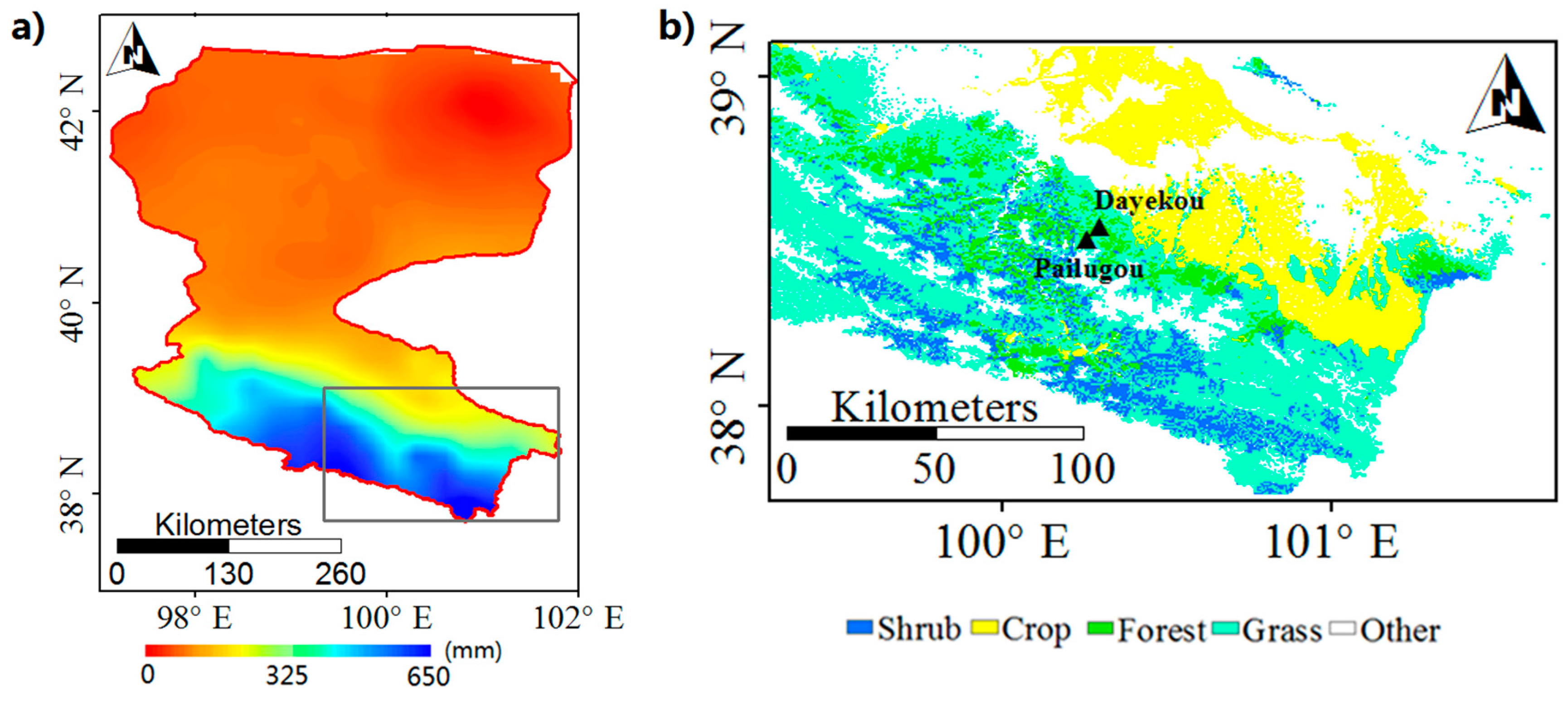
2.1. Study Area

The study area (37.71°N–39.11°N, 99.29°E–101.68°E) is located in the upper reach of the Heihe River Basin in the Northwestern China (Figure 1). This is an arid region characterized by a dry continental climate with the annual mean temperature about 2.0 °C. The annual precipitation varies from 400 to 600 mm [10], compared with a high annual potential evaporation of more than 2000 mm. This area is at approximately 1500 m above sea level and has a rugged terrain. The landscapes are diverse and the main vegetation types are forest, shrub, crop, and grass.

2.2. Data

The aim of this study is to estimate vegetation rainfall interception at very high resolution using the RS-Gash model. Forcing data and remote sensing data, such as precipitation, are required inputs into the model. In addition, filed measurements are also needed to evaluate model performance.

2.2.1. In Situ Measurements of Vegetation Rainfall Interception

Rainfall interception was measured from June to September in 2008 at Dayekou (38.507°N, 100.258°E) and Pailugou (38. 543°N, 100.295°E) forest experimental sites [1] in the upper reach of the Heihe River Basin (locations of both sites are denoted in Figure 1b). During the experiment, rainfall, throughfall, and stemflow were measured. Gross rainfall is measured on the open ground beside the tree canopy. Throughfall is measured under trees in the forest using several troughs. Stemflow collected from several trees using coiled pipes randomly selected and calculated by taking the average tree density of the sites into account [8], and the interception loss for every rainfall event was estimated as the residual of the gross rainfall, throughfall, and stemflow. Interception ratio (%) is also calculated to evaluate the model performance.

2.2.2. Forcing Data

In this study, the hourly forcing data from the Weather Research and Forecasting model (WRF) simulation [11], provided by the Heihe Plan Science Data Center, is used to drive the RS-Gash model. The forcing data includes wind speed at 10 m height, air temperature, specific humidity, air pressure, as well as downward short-wave and long-wave radiation fluxes at 2 m height with a spatial resolution of 5 km. Field validation shows that the average mean bias error (MBE) of the hourly surface temperature, surface pressure, relative humidity, wind speed, downward shortwave radiation and downward longwave are −0.16 °C, −6.62 hPa, −5.14%, 0.26 m/s, 33.0 W/m², and −6.44 W/m², and the average correlation coefficients (R) of them are 0.96, 0.97, 0.70, 0.26, 0.91, and 0.60, respectively [12]. The spatial resolution of 5 km was downscaled to 30 m using the bilinear resampling method for all variables.

2.2.3. Remote Sensing Data

Tropical Rainfall Measuring Mission (TRMM) 3B42 Version 7 precipitation with a spatial resolution of 0.25° and a temporal resolution of 3 h, is used in this study. The TRMM 3B42 V7 precipitation product provides an estimate of precipitation from merged precipitation radar (PR), TRMM Microwave Imager (TMI), Special Sensor Microwave Imager (SSM/I), and Geostationary Orbiting Environmental Satellite (GOES) infrared (IR) measurements. The TRMM product covering the latitude band 50°N–50°S was provided by the TRMM Multi-satellite Precipitation Analysis by combining precipitation estimates from multiple satellites and rain gauge analyses since 1998 [13,14]. The daily precipitation is obtained by summing up all eight sets of three-hourly TRMM precipitation in one day. Some studies show that TRMM monthly product has higher reliability than at three-hourly and daily products [14]. Reprojection and bilinear interpolation method were also used to obtain data at a spatial resolution of 30 m and temporal resolution of 1 h.

The VAI at 30 m resolution every 16 days was retrieved from Landsat ETM+ images every 16 days using the hybrid model of canopy reflectance to be described in Section 3.2. The raw data in each ETM+ band (except thermal and panchromatic) was converted to reflectance using an atmospheric model prior to the VAI calculation. The ETM+ sensor has been calibrated vicariously using Earth targets, such as Railroad Valley (Thome, 2001; Thome et al., 2004), and cross-calibrated with multiple sensors (Teillet et al., 2001, 2006, 2007; Thome et al., 2003; Chander et al., 2004b, 2007b, 2008). Daily values of VAI were obtained using the bilinear resampling method for time series.

The land cover map (Figure 1b) at 30 m resolution used in this study is also based on Landsat ETM+ images using the decision tree method.

3. Methods

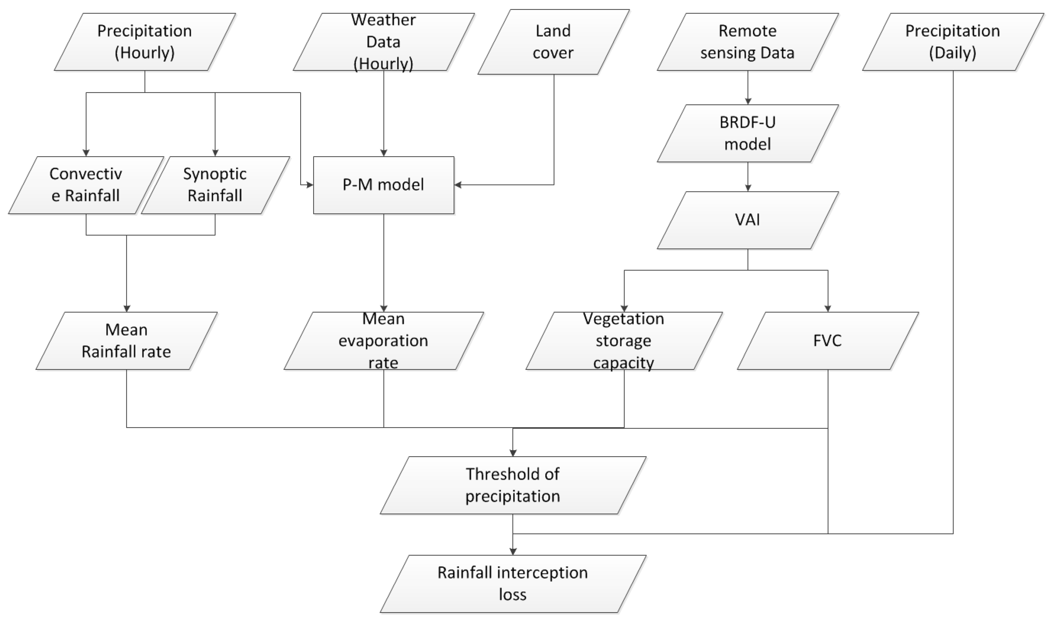
3.1. RS-Gash Analytical Model

To calculate vegetation rainfall interception (I, mm) at the regional scale, the RS-Gash model [8,9]) was used. RS-Gash model was a modified Gash model [7] using remote sensing products as inputs, making it applicable at regional and daily scales. At the coarse scale (such as 1 km), the RS-Gash model describes the heterogeneity of vegetation distribution on the sub-pixel scale by the Poisson distribution, for the vegetation structural parameter can significantly affect the vegetation rainfall interception. However, it is reasonable that the impact of vegetation heterogeneity can be neglected at the fine spatial scale (such as 30 m), considering that it is reasonable to treat a pixel in such a fine spatial scale as a pure pixel. Hence, the RS-Gash model applied at the very high resolution, can be simplified as follows:

$$\{\begin{array}{c}\mathrm{I}=\mathrm{FVC}·{\mathrm{P}}_{G}for\left({\mathrm{P}}_G<P_G^{\prime }\right)\\ I=\mathrm{FVC}·P_G^{\prime }+\left(\mathrm{FVC}·\overline{E_V}/\overline{R}\right)\left({\mathrm{P}}_G-P_G^{\prime }\right)for\left({\mathrm{P}}_G>P_G^{\prime }\right)\end{array}$$

(1)

where $\overline{E_V}$ (mm h⁻¹) is the mean evaporation rate per unit vegetation coverage area from saturated vegetation surfaces, including evaporation rate from canopy and stem; $\overline{R}$ (mm h⁻¹) is the mean rainfall rate which is high enough to make the vegetation saturated; the ratio of $\overline{E_V}$ over $\overline{R}$ is the monthly mean (one per month), and is assumed to be equal for all storms during one month; FVC is the Fractional Vegetation Cover; ${\mathrm{P}}_G$ (mm) is the gross rainfall; $P_G^{\prime }$ (mm) is the threshold value of precipitation required to saturate the vegetation, and is given by:

$$P_G^{\prime }=-\frac{\overline{R}}{\overline{E_V}}·\frac{S_{veg}}{\mathrm{FVC}}·\ln \left(1-\frac{\overline{E_V}}{\overline{R}}\right)$$

(2)

$$S_{veg}=S_V·VAI$$

(3)

where $S_{veg}$ (mm) is vegetation storage capacity, including canopy and stem storage capacity, which is assumed linearly related with vegetation area; $S_V$ (mm) is the specific vegetation storage, defined as the depth of water retained by vegetation per unit vegetation area. The values of $S_V$ is set to 0.25, 0.15, 0.55, 0.06, and 0.06 for the needleleaf forest, broadleaf forest, shrub, grass and crop, respectively [9]; VAI (m² m⁻²) is calculated using a hybrid model of canopy reflectance propose Xu, et al. [15]. All the rainfall intercepted by vegetation is assumed to be evaporated into atmosphere, and there are several evaporation components in the whole process that are described by Equation (1): (1) the $\mathrm{FVC}·{\mathrm{P}}_G$ part is for small storms insufficient to saturate the vegetation; (2) the $\mathrm{FVC}·P_G^{\prime }$ part is the interception from rainfall beginning to the vegetation saturated, which could be separated into evaporation during vegetation wetting up (including leaves and trunks), and vegetation storage after saturation, which will evaporate after rainfall ceases; and (3) the $\left(\mathrm{FVC}·\overline{E_V}/\overline{R}\right)\left({\mathrm{P}}_G-P_G^{\prime }\right)$ part is the evaporation from saturation until rainfall cessation (including from leaves and trunks).

Figure 2 illustrates the process of calculating rainfall interception loss in the RS Cash model and is described in details as follows.

(1)

Divide rainfall events into convective (high intensity) and synoptic (low intensity) ones using a threshold of rainfall rate of 2 mm h⁻¹ [5,9]; and calculate their monthly mean rainfall rate separately;

(2)

Calculate evaporation using the Penman-Monteith model [16] using the hourly forcing data from WRF model:

λE = (∆R_n + ρc_pD/r_a)(∆ + γ)⁻¹

(4)

where E (kg m⁻² s⁻¹) is the evaporation rate; λ (J kg⁻¹) is the latent heat of vaporization; r_a (s m⁻¹) is the aerodynamic resistance; R_n (W m⁻²) is the net radiation; c_p (J kg⁻¹ K⁻¹) is the specific heat capacity of air at constant pressure; D (Pa) is the vapor pressure deficit; γ (Pa K⁻¹) is the psychrometric constant; ∆ (Pa K⁻¹) is the slope of the saturation vapor pressure curve at air temperature; and ρ (kg m⁻³) is the density of air;

(3)

The vegetation storage capacity and FVC are obtained based on VAI retrieved from very high resolution remote sensing image (see Section 3.2);

(4)

Finally, the vegetation rainfall interception is calculated from the RS-Gash model with parameters and input variables acquired in the previous several steps.

3.2. VAI Retrieval Model and FVC

The VAI was retrieved using the unified model of bidirectional reflectance distribution function for the vegetation canopy (BRDF-U model) proposed by Xu et al. (2017). Different from other BRDF models, the BRDF-U model considers the reflectance from all parts of vegetation. Hence, it can be used to retrieve the VAI. In the BRDF-U model, the canopy reflectance (from green leaves, dry leaves, branches, stem, and trunk) is approximated as the sum of the single scattering reflectance arising from the sun, ${\rho }^1$, and the multiple scattering reflectance arising from the canopy, ${\rho }^m$. According to the geometrical optical model and the recollision probability theory, a new analytical expression of ${\rho }^1$ and ${\rho }^m$ is obtained, respectively. The model was validated using ground measurements of maize and black spruce forest and the reliability of the model was proved [15]. After the model built, the look-up-tables (LUT) method can be used to retrieve the VAI [17].

The FVC is calculated as:

$$\mathrm{FVC}=1-e^{-{\lambda }_0\frac{G}{\mu }VAI}$$

(5)

where λ₀ is the Nilson parameter considering vegetation clumping effect, G is the mean projection of a unit of vegetation area onto the plane perpendicular to the incident beam direction, μ is the cosine of the observation zenith angle. And μ can be calculated by the satellite observing angle. G and λ₀ can be inferred from the prior knowledge [18].

4. Results

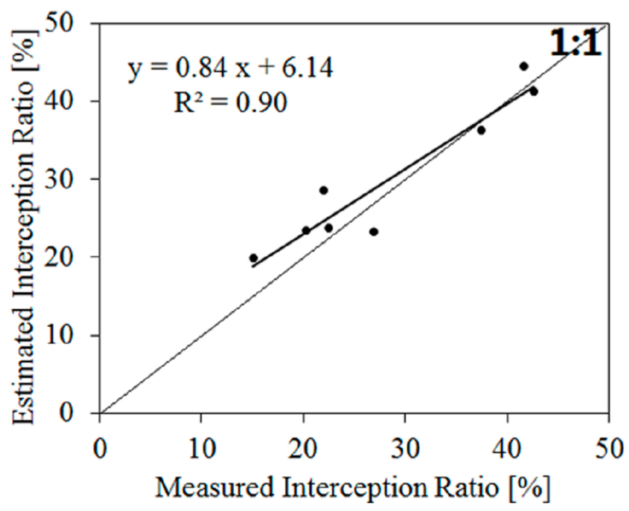
4.1. Field Validation

At 30 m resolution grid cells, it is reasonable to treat most pixels as pure pixels that are covered by a single type of vegetation entirely. Hence, the vegetation rainfall interception has little effect from mixed pixels and the validation can performed reasonably. The statistics of estimated and measured monthly interception ratio (%) at the two sites in 2008 are summarized in

Table 1. Statistics of estimated and measured monthly interception ratio (%) of the two forest sites from June to September of 2008.

Month/Year	Dayekou		Pailugou
	Estimated	Measured	Estimated	Measured
June 2008	26.9	23.2	41.7	44.5
July 2008	20.3	23.4	37.5	36.3
August 2008	15.1	19.9	42.6	41.3
September 2008	22.5	23.7	22.0	28.5
Mean	21.2	22.6	35.9	37.7
STD	4.9	1.8	9.6	7.0
RMSE	3.46		3.65

. For both sites, the difference of the mean interception ratio between the estimated and measured values is less than 2%. The STD (standard deviation) is less than 10%, and the RMSE is less than 3.7%, indicating the model’s strong stability and reliability. The estimated and measured interception ratios agreed well with each other, with R² of 0.9 (Figure 3). Due to the factor that more than 95% rainfall and more than 95% precipitation (rainfall and snowfall) occur from May to October, making the total interception during this period approximately equal to the annual one. Therefore, in this study we treat the accumulated interception of these months as its annual value. Figure 4 shows the spatial distribution of the annual interception loss and interception ratio. A comparison of this spatial pattern with that of precipitation and land cover types (Figure 1a,b) suggests that the south/north contrast is mainly caused by the precipitation, and the west/east contrast is mainly controlled by land cover types. Limited to in situ measurements in the study area, the performance for other vegetation types cannot be verified directly. We want to state that the Gash model has been successfully used in different types of vegetation, including rainforest, conifers, mixed conifer, shrubs, and crops [19]. Hence, it is reasonable to assume that the RS-Gash model is also suitable for estimating the interception loss of shrub, grass, and crop for which is a modification of the Gash model for estimating interception loss at the regional scale.

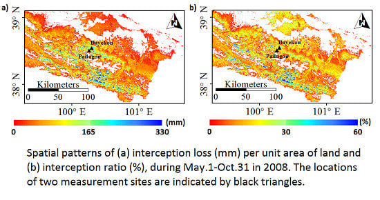
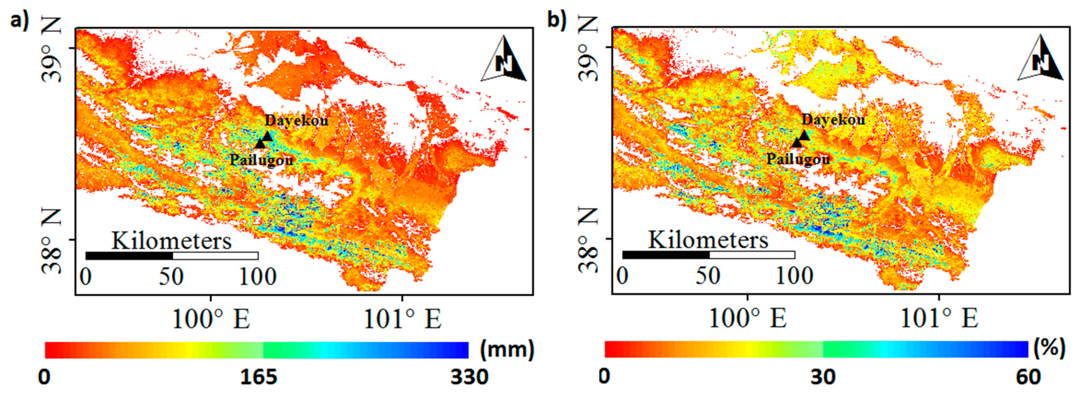
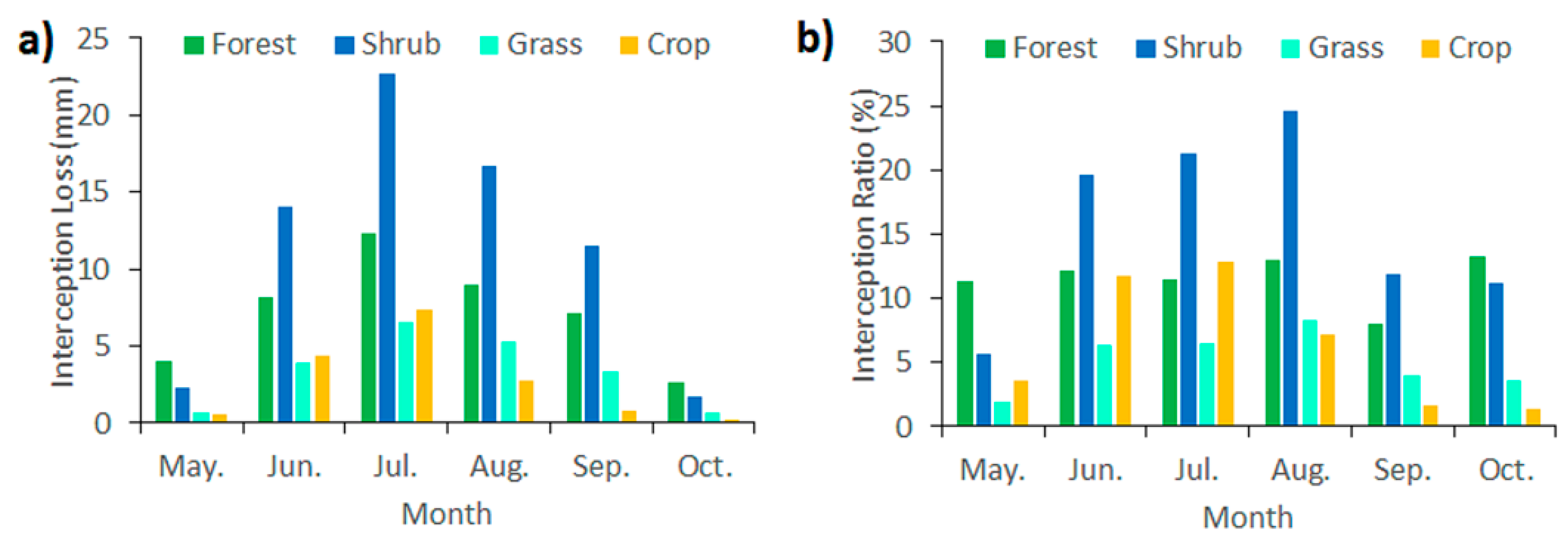
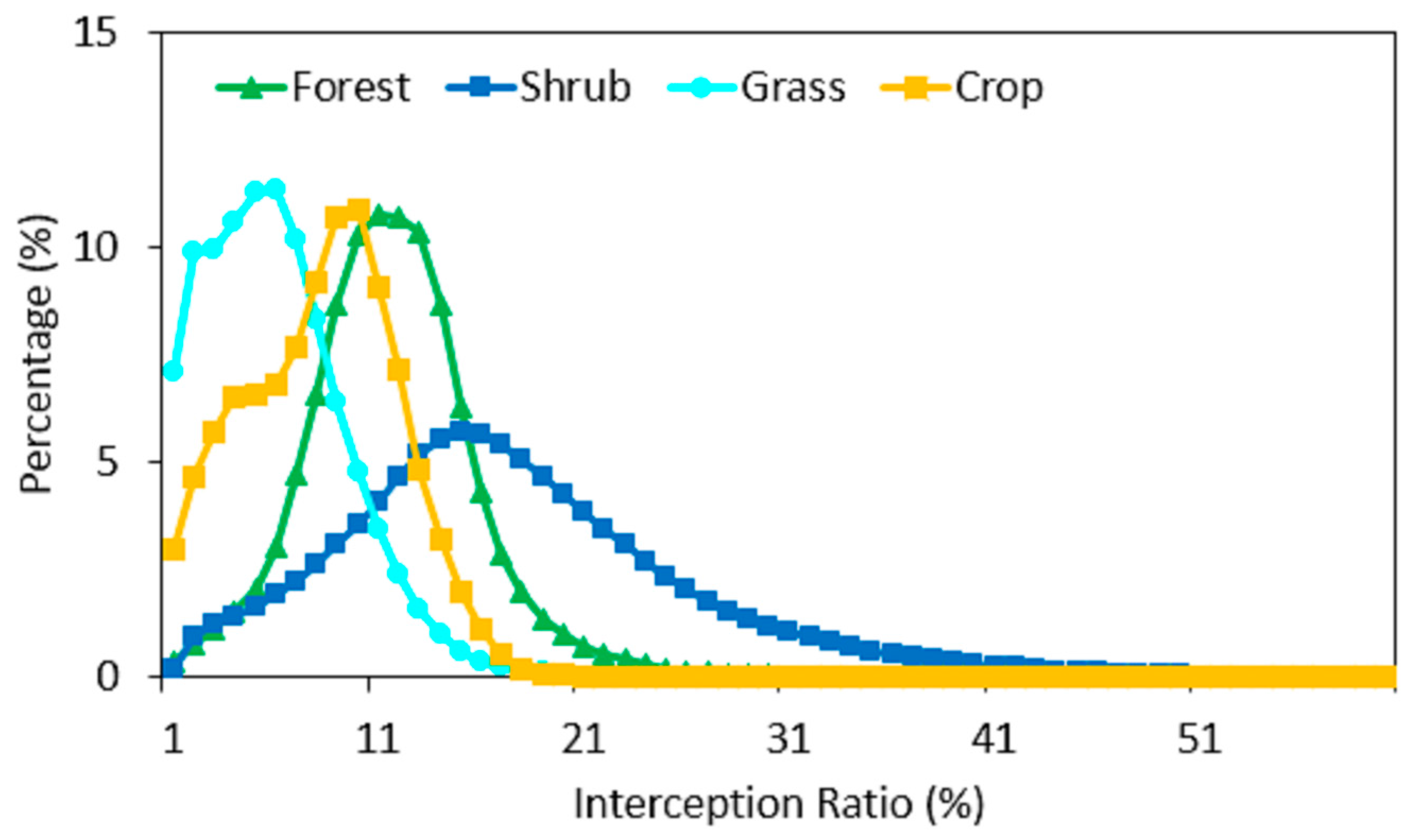
4.2. The Variation of Interception across Different Vegetation Types

Forest, shrub, grass, and crop are chosen to demonstrate the difference of interception by different types of vegetation. Monthly interception loss and interception ratio of the four vegetation types show the similar variation (Figure 5). We take the interception ratio as the example. The interception ratio is much higher in summer than in spring and fall for all vegetation types, due to the higher VAI and higher potential evapotranspiration in summer. The interception ratios of forest and shrub are much higher than those of grass and crop, due to their higher ability to hold water resulting from the higher vegetation storage capacity for a certain rainfall event. The interception ratio for shrub is higher than for forest from June to September, however, in May and October it is just the inverse. The reason is that the evergreen forest has much larger VAI than shrub in these months. Due to the harvest for crop, the crop interception ratio is higher first and then becomes lower than grass. In summary, the results show that the VAI, potential evapotranspiration and precipitation are the main controlling factors of interception. The probability density function of the interception ratio is shown in Figure 6. As shown in

Table 2. The averaged interception loss and interception ratio of different vegetation at fine and coarse resolution for the whole study area.

	Interception Loss (mm, Fine)	Interception Loss (mm, Coarse)	Interception Ratio (%, Fine)	Interception Ratio (%, Coarse)
Forest	43.41	55.90	11.17	14.63
Shrub	69.06	60.65	17.31	15.33
Crop	20.49	13.30	5.61	4.37
Grass	16.11	10.47	7.48	4.79

, magnitude order of the interception loss per unit area of different vegetation types from high to low is: shrub (69.06 mm), forest (43.41 mm), crop (20.49 mm), and grass (16.11 mm). The averaged interception ratios are: 17.31%, 11.17%, 7.48%, and 5.61%, for shrub, forest, crop, and grass, respectively.

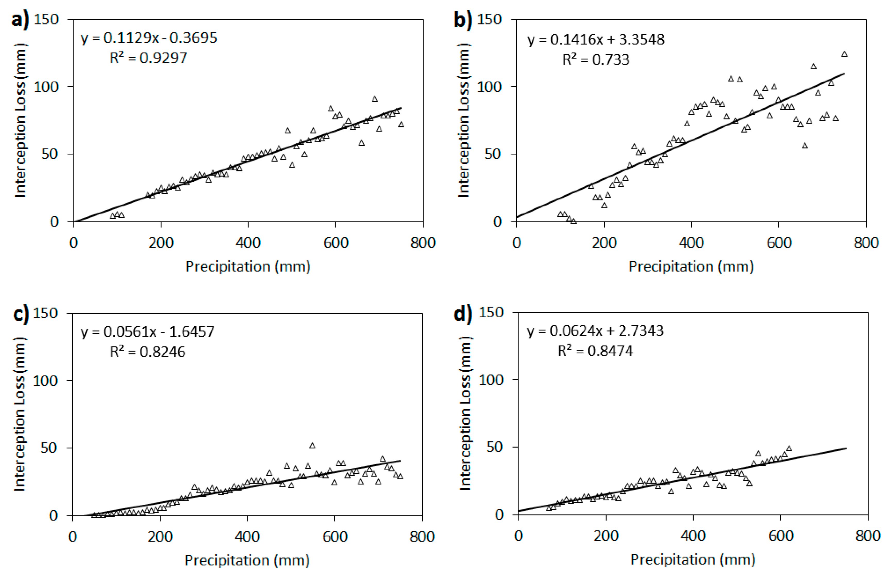
4.3. The Relationship between Interception and Precipitation

The relationship between the interception loss and the precipitation from May to October for different vegetation types are shown in Figure 7. The interception loss and precipitation are averaged, hence the figure could show the relationship at regional (about 1050 km²) and annual scales. All of the R² higher than 0.7 shows that there are a significant linear relationship between interception loss and precipitation at regional and annual scales. However, the relationship between the annual interception ratio and precipitation is not very obvious (figure not shown). The linear relationship is strongest for the forest, followed by the crop and the grass, with the shrub is the weakest, indicating that the change of daily VAI and difference of vegetation storage capacity are the main factors affecting the relationship between interception and precipitation, for that the forest has smoother VAI change, and shrub has much larger vegetation storage capacity. These empirical relationship might be useful for calculating the interception loss under different precipitation inputs for hydrological model simulation in the Heihe River Basin of China. However, caution is needed when applying this relationship beyond the Heihe River Basin.

5. Discussion

This study only focused on the vegetation rainfall interception, since the snowfall interception is very low in our study area and is beyond the scope of this paper. We had two in situ measurements in the forest sites from June to September in 2008 to validate our model. The validation was performed based on the two datasets. Meanwhile, we only validate the interception ratio at the monthly scale in this study, since the TRMM precipitation is comparable with the field measurements at this scale and the ratio is helpful to minimize the discrepancy between TRMM and field precipitation. Hence, the absolute magnitude of interception loss at event timescale or the value of interception loss is difficult to validate directly, as it largely depends on the accuracy of the input precipitation data.

To understand the scale effect of the vegetation rainfall interception, the rainfall interception products with fine resolution of 30 m is reprojected and resampled to 1 km and compared with the results from MODIS data derived at 1 km resolution (called the coarse product, and the product at 30 m is called the fine product). The MODIS coarse product was downloaded from the Cold and Arid Regions Science Data Center (http://westdc.westgis.ac.cn/data/), and produced from the RS-Gash model as used in this paper, with the same forcing data and precipitation data as in this study, except the VAI that was calculated from the MODIS product using an empirical method. Figure 8 shows that the rainfall interception loss and interception ratio at high resolution are spatially consistent with the coarse one (see: Figure 8a,b,d,e). The difference in spatially-averaged values between the two spatial scales are less than 5 mm and 3% for the interception loss and interception ratio, respectively, indicating that the RS-Gash model has strong flexibility across various spatial scales. However, there are still some regions showing low consistency, especially in the southern portion of the study area. Table 2 shows the averaged interception loss and interception ratio of different vegetation with fine and coarse resolutions for the whole study area. At either fine or coarse scale, the magnitude of the interception loss and interception ratio show the same order. In addition, except for the forest, the averaged interception loss and interception ratio of other vegetation types are higher at the fine scale than at the coarse scale (Table 2). Normally, the rainfall interception are affected by saturated evapotranspiration, gross of rainfall, structural parameters of vegetation (such as: VAI) and the land cover. Under different scales, the saturated evapotranspiration and gross rainfall have little difference. Hence, the difference is caused by that of VAI and land cover. Comparison of the original and reconstructed MODIS optical products are shown in Figure 8.

Compared with the estimation at coarse resolution, the estimated vegetation rainfall interception at very high resolution using the RS-Gash model could reduce the uncertainties significantly. As a remote sensing-based model, the RS-Gash model has better computational efficiency of hydrological models which have many complex models to describe the process. Hence, it will be very useful to obtain rainfall interception with high reliability at a large scale. As meteorology and vegetation parameters are considered, the model has good applicability under different climates and land cover.

6. Conclusions

In this study, an analytical interception model named RS-Gash model was used to obtain the high-resolution vegetation interception. To improve the performance of the model, the BRDF-U model based on remote sensing was used to retrieve the VAI, which is a key variable for the RS-Gash model, instead of the empirical methods. The rainfall interception for four types of vegetation were estimated and validated in the upper reach of the Heihe River Basin of China. This study is the first to try to obtain the vegetation rainfall interception at very high resolution. The RMSE and R² of the interception ratio are 3.7% and 0.9, respectively, showing that the model has strong stability and reliability at this scale. We found that the magnitude order of the interception loss per unit area of different vegetation types from high to low is: shrub (69.06 mm), forest (43.41 mm), crop (20.49 mm), and grass (16.11 mm) in the Heihe River Basin. The regression shows that there are strong linear relationships between vegetation rainfall interception and the gross rainfall, with the strongest for the forest, followed by the crop and the grass, and the weakest for the shrub. However, this relationship might be different at different zones. There are four factors affecting the vegetation rainfall interception: saturated evapotranspiration, gross rainfall, VAI, and the land cover. In addition, there are strong scale effects for VAI and land cover. To obtain reliable vegetation rainfall interception, the RS-Gash model applied at fine scale is necessary. The knowledge of the interception is of great importance for the runoff simulating and the flood forecasting. Satellite-based analytical methods could hold considerable potential in providing reliable relevant information at high spatial resolution, as shown in this study. In the future, we plan to use this model to drive the hydrological model in simulating runoff and to investigate long-term changes in the vegetation rainfall interception based on a longer record of years using this model.

References

1. Li, X.; Li, X.; Li, Z.; Ma, M.; Wang, J.; Xiao, Q.; Liu, Q.; Che, T.; Chen, E.; Yan, G.; et al. Watershed Allied Telemetry Experimental Research. Watershed Allied Telemetry Experimental Research. J. Geophys. Res. Atmos. 2009, 114. [Google Scholar] [CrossRef]
2. Herbst, M.; Rosier, P.T.W.; McNeil, D.D.; Harding, R.J.; Gowing, D.J. Seasonal variability of interception evaporation from the canopy of a mixed deciduous forest. Agric. For. Meteorol. 2008, 148, 1655–1667. [Google Scholar] [CrossRef]
3. Van Dijk, A.I.J.M.; Bruijnzeel, L.A. Modelling rainfall interception by vegetation of variable density using an adapted analytical model. Part 2. Model validation for a tropical upland mixed cropping system. J. Hydrol. 2001, 247, 239–262. [Google Scholar] [CrossRef]
4. Levia, D.F.; Frost, E.E. Variability of throughfall volume and solute inputs in wooded ecosystems. Prog. Phys. Geogr. 2006, 30, 605–632. [Google Scholar] [CrossRef]
5. Miralles, D.G.; Gash, J.H.; Holmes, T.R.H.; de Jeu, R.A.M.; Dolman, A.J. Global canopy interception from satellite observations. J. Geophys. Res. Atmos. 2010, 115. [Google Scholar] [CrossRef]
6. Mo, X.G.; Liu, S.X.; Lin, Z.H.; Zhao, W.M. Simulating temporal and spatial variation of evapotranspiration over the Lushi basin. J. Hydrol. 2004, 285, 125–142. [Google Scholar] [CrossRef]
7. Gash, J.H.C.; Lloyd, C.R.; Lachaud, G. Estimating Sparse Forest Rainfall Interception with an Analytical Model. J. Hydrol. 1995, 170, 79–86. [Google Scholar] [CrossRef]
8. Cui, Y.; Jia, L. A Modified Gash Model for Estimating Rainfall Interception Loss of Forest Using Remote Sensing Observations at Regional Scale. Water 2014, 6, 993–1012. [Google Scholar] [CrossRef]
9. Li, X.; Cheng, G.D.; Liu, S.M.; Xiao, Q.; Ma, M.G.; Jin, R.; Che, T.; Liu, Q.H.; Wang, W.Z.; Qi, Y.; et al. Heihe Watershed Allied Telemetry Experimental Research (HiWATER): Scientific Objectives and Experimental Design. Bull. Am. Meteorol. Soc. 2013, 94, 1145–1160. [Google Scholar] [CrossRef]
10. Cui, Y.K.; Jia, L.; Hu, G.C.; Zhou, J. Mapping of Interception Loss of Vegetation in the Heihe River Basin of China Using Remote Sensing Observations. IEEE Geosci. Remote Sens. Lett. 2015, 12, 23–27. [Google Scholar]
11. Pan, X.D.; Li, X.; Shi, X.K.; Han, X.J.; Luo, L.H.; Wang, L.X. Dynamic downscaling of near-surface air temperature at the basin scale using WRF-a case study in the Heihe River Basin, China. Front. Earth Sci. 2012, 6, 314–323. [Google Scholar] [CrossRef]
12. Pan, X.D.; Li, X. Validation of WRF model on simulating forcing data for Heihe River Basin. Sci. Cold Arid Reg. 2011, 03, 344–357. [Google Scholar]
13. Kummerow, C.; Simpson, J.; Thiele, O.; Barnes, W.; Chang, A.T.C.; Stocker, E.; Adler, R.F.; Hou, A.; Kakar, R.; Wentz, F.; et al. The status of the Tropical Rainfall Measuring Mission (TRMM) after two years in orbit. J. Appl. Meteorol. 2000, 39, 1965–1982. [Google Scholar] [CrossRef]
14. Huffman, G.J.; Adler, R.F.; Bolvin, D.T.; Gu, G.J.; Nelkin, E.J.; Bowman, K.P.; Hong, Y.; Stocker, E.F.; Wolff, D.B. The TRMM multisatellite precipitation analysis (TMPA): Quasi-global, multiyear, combined-sensor precipitation estimates at fine scales. J. Hydrometeorol. 2007, 8, 38–55. [Google Scholar] [CrossRef]
15. Xu, X.; Fan, W.; Li, J.; Zhao, P.; Chen, G. A unified model of bidirectional reflectance distribution function for the vegetation canopy. Sci. China Earth Sci. 2017, 60, 463–477. [Google Scholar] [CrossRef]
16. Monteith, J.L. Evaporation and environment. Symp. Soc. Exp. Biol. 1965, 19, 205–223. [Google Scholar] [PubMed]
17. Liao, Y.; Fan, W.; Xu, X. Algorithm of Leaf Area Index Product for HJ-CCD over Heihe River Basin. In Proceedings of the 2013 IEEE International Geoscience and Remote Sensing Symposium (IGARSS), Melbourne, Australia, 21–26 July 2013; pp. 169–172. [Google Scholar]
18. Cui, Y.K.; Zhao, K.G.; Fan, W.J.; Xu, X.R. Retrieving crop fractional cover and LAI based on airborne Lidar data. J. Remote Sens. 2011, 15, 1276–1288. [Google Scholar]
19. Muzylo, A.; Llorens, P.; Valente, F.; Keizer, J.J.; Domingo, F.; Gash, J.H.C. A review of rainfall interception modelling. J. Hydrol. 2009, 370, 191–206. [Google Scholar] [CrossRef]
Figure 1. Location of the study area: (a) the distribution of mean annual precipitation from TRMM during 2008–2011 in the Heihe River Basin; and (b) land cover types at 30 m resolution with two measurement sites (Dayekou and Pailugou) indicated by black triangles.
Remotesensing 09 00661 g001
Figure 2. Flowchart of the RS-Gash model.
Remotesensing 09 00661 g002
Figure 3. Estimated versus measured interception ratio.
Remotesensing 09 00661 g003
Figure 4. Spatial patterns of (a) interception loss (mm) per unit area of land and (b) interception ratio (%), during 1 May–31 October 2008. The locations of two measurement sites are indicated by black triangles.
Remotesensing 09 00661 g004
Figure 5. The monthly value of: (a) interception loss (mm), and (b) interception ratio (%) for four different vegetation types in the study area.
Remotesensing 09 00661 g005
Figure 6. The probability density function of the interception ratio. Values are averaged from May to October in 2008.
Remotesensing 09 00661 g006
Figure 7. The relationship between annual interception loss and precipitation at regional scale for (a) forest, (b) shrub, (c) grass, and (d) crop.
Remotesensing 09 00661 g007
Figure 8. Comparison of the two rainfall interception products. (ac) are the interception loss (mm) resampled from 30 m to 1 km, the interception loss (mm) at 1 km from MODIS product, and the histogram of the difference between (a) and (b), respectively; (df) are the interception ratio (%) resampled from 30 m to 1 km, the interception ratio (%) at 1 km from the MODIS product, and the histogram of the difference between (d) and (e), respectively.
Remotesensing 09 00661 g008