Urban Area Extraction by Regional and Line Segment Feature Fusion and Urban Morphology Analysis


1
Department of Computer Science and Technology, East China Normal University, Shanghai 200241, China
2
School of Remote Sensing and Information Engineering, Wuhan University, Wuhan 430079, China
3
State Key Laboratory of Information Engineering in Surveying, Mapping and Remote Sensing, Wuhan University, Wuhan 430079, China
*
Authors to whom correspondence should be addressed.
Remote Sens. 2017, 9(7), 663; https://doi.org/10.3390/rs9070663
Submission received: 26 April 2017
/
Revised: 7 June 2017
/
Accepted: 26 June 2017
/
Published: 28 June 2017
Abstract
:Urban areas are a complex combination of various land-cover types, and show a variety of land-use structures and spatial layouts. Furthermore, the spectral similarity between built-up areas and bare land is a great challenge when using high spatial resolution remote sensing images to map urban areas, especially for images obtained in dry and cold seasons or high-latitude regions. In this study, a new procedure for urban area extraction is presented based on the high-level, regional, and line segment features of high spatial resolution satellite data. The urban morphology is also analyzed. Firstly, the primitive features—the morphological building index (MBI), the normalized difference vegetation index (NDVI), and line segments—are extracted from the original images. Chessboard segmentation is then used to segment the image into the same-size objects. In each object, advanced features are then extracted based on the MBI, the NDVI, and the line segments. Subsequently, object-oriented classification is implemented using the above features to distinguish urban areas from non-urban areas. In general, the boundaries of urban and non-urban areas are not very clear, and each urban area has its own spatial structure characteristic. Hence, in this study, an analysis of the urban morphology is carried out to obtain a clear regional structure, showing the main city, the surrounding new development zones, etc. The experimental results obtained with six WorldView-2 and Gaofen-2 images obtained from different regions and seasons demonstrate that the proposed method outperforms the current state-of-the-art methods.
1. Introduction
Urban areas are the main areas of human activity, and they have a great impact on the Earth’s land-surface change and the ecological environment. An urban distribution map can reflect the degree of regional urbanization, and is also the most basic geographic data source for urban planning, development, and change monitoring [1]. In recent decades, remote sensing has been the main approach to efficient urban land-cover mapping. Considerable efforts have been made to improve the accuracy of urban land-cover mapping [2,3,4,5,6,7,8]. A number of different approaches have been proposed in recent years for automatically detecting urban areas from remotely sensed images [9,10].
In the early years, only low or medium spatial resolution images were available to the general public and researchers [11,12]. In these images, the characteristics of urban areas are mainly identified by impervious surfaces [9] or built-up areas [10]. In previous research, the traditional pattern recognition and classification methods, such as spectral unmixing [13], artificial neural networks [14], support vector machine, random forest [15,16,17], and so on. However, the results of these (supervised) methods depend on the quality of the selected training samples. Furthermore, their collection is a time-consuming task.
Many different indices for impervious surfaces and built-up areas have been presented, including the urban index (UI) [18], the normalized difference built-up index (NDBI) [19], the normalized difference impervious surface index (NDISI) [20], the enhanced built-up and bareness index (EBBI) [21], and the combinational build-up index (CBI) [9]. These indices are quick, simple, and convenient in practical applications. However, these indices face a variety of challenges. For example, they are subject to seasonal variation, and it can be difficult to distinguish between built-up and bare land areas. These indices may also require special bands, or they may be sensor-dependent [9]. In [22], multitemporal synthetic aperture radar (SAR) data were used to define the built-up index.
With the increase of the spatial resolution of images, the significant spatial structure information of the land surface can be used to improve the accuracy of urban area extraction [23,24,25]. Urban scenes have unique textures when compared to natural scenes, and this can be exploited to classify, i.e., gray-level co-occurrence matrix (GLCM) [26], the normalized gray-level histogram [27], and the Gabor wavelet [28]. Pesaresi et al. [10] proposed a robust built-up area presence index, namely, the PanTex index, which is an anisotropic rotation-invariant textural measure derived from panchromatic satellite data. In [29], morphological multiscale operators were used to undertake urban texture recognition.
In all the references reviewed, it was found that most of the image resolutions (e.g., Moderate Resolution Imaging Spectroradiometer (MODIS), Landsat 8, Landsat Thematic Mapper (TM), and SPOT-5) used for urban area extraction are lower than 5 m [9,11]. In addition, with the increase of the resolution, the extraction accuracy of urban areas is reduced [10], for the following reasons. Urban areas are a complex combination of various land-cover types (vegetation, buildings with different colors, roads, water, parking lots, etc.), and they show a variety of land-use structures and spatial layouts. Furthermore, impervious surfaces (buildings, roads, parking lots, and so on) dominate urban areas. Thus, in low- and medium-resolution images, urban areas are mainly manifested by impervious surfaces with similar spectral information. With the increase of the image resolution, the small objects of the non-impervious surface land-cover types, such as vegetation, water, grass, soil, and so on, are clearly displayed in the images, which brings great challenges to the urban area extraction, especially for high-resolution remote sensing images containing only four channels (red (R), green (G), blue (B), and near-infrared (NIR)).
An urban place can be regarded as a spatial concentration of people whose lives are organized around nonagricultural activities [30]. Urban areas are created through urbanization, and are categorized by urban morphology as cities, towns, conurbations, or suburbs. “Built-up area” is a term used primarily in urban planning, real estate development, building design, and the construction industry. It encompasses the following: firstly, a developed area, i.e., any land on which buildings are present, normally as part of a larger development; and, secondly, a “gross building area” (construction area). Impervious surfaces are mainly artificial structures (pavements, roads, sidewalks, driveways, and parking lots) that are covered by impenetrable materials such as asphalt, concrete, brick, and stone. It is clear that urban areas partly equate to built-up areas, and impervious surfaces are not equivalent to urban areas, which also contain green spaces. Due to one pixel covering a large area of ground in low- and medium-resolution images, and the fact that impervious surfaces dominate urban zones, urban areas and impervious surfaces have similar spectral information. The extraction of urban areas, built-up areas, and impervious surfaces is indistinguishable when using low- and medium-resolution images. However, in all the references reviewed, we found that these concepts of urban areas, built-up areas, and impervious surface are usually not distinguished in high spatial resolution imagery [10,31].
The aim of this paper is to extract urban areas from high spatial resolution images, and to simultaneously analyze the spatial structure distribution of the urban areas. This task is faced with many challenges:
Firstly, urban areas contain various land-cover types (vegetation, buildings, roads, water bodies, parking lots, green spaces, bare soil, shadow, etc.) at microscopic (local spatial units) spatial extent, and complex combinations of the many land-cover types can be clearly seen in high spatial resolution images.
Secondly, many of the impervious land-cover types of urban areas, such as buildings, have similar spectral information to the impervious land-cover types of non-urban areas, such as bare land, sand, or rock, especially for the images obtained in dry and cold seasons or high-latitude regions.
Thirdly, urban morphology shows diversity in the macroscopic spatial extent. Urban areas are categorized by urban morphology as cities, towns, conurbations, or suburbs, which show a wide variety of land-use structures and spatial layouts. Furthermore, with the development of urban planning, the greening of urban areas is becoming more common, which can result in confusion with rural areas.
Wilkinson [32] and Li et al. [33] demonstrated that new algorithms can improve the accuracy of land-cover and land-use mapping, but the improvement is limited. Gong et al. [34] suggested that more effort should be made to include new features to improve the accuracy of land-cover mapping. In addition, recent studies of deep learning have demonstrated that a combination of low-level features can form a more abstract high-level representation of the attribute categories or characteristics, and can significantly improve the recognition accuracy [35,36].
The aim of this study is to extract the urban areas from high spatial resolution images. In order to solve the above problems, a new approach is proposed based on small spatial units and high-level features extracted from the primitive features, such as regional features and line segments. This approach is much easier than the fusion of features at the land-use level. Classification and urban spatial structure analysis are then performed for all the non-overlapping small spatial units of the entire image (the flow chart of the proposed approach is shown in Section 3). The contributions of this paper are as follows:
- (1)
- The proposed method has the advantage of strong fault tolerance. The multiple high-level features, which are extracted from the primitive features in microscopic spatial extents, are used to describe the complex spectral and spatial properties of urban areas.
- (2)
- Line segments and their spatial relationship with regional features are used to describe the urban area.
- (3)
- Urban morphology analysis is undertaken at a macroscopic spatial extent, based on morphological spatial pattern analysis (MSPA).
The rest of this paper is organized as follows. The study areas and remotely sensed data are introduced in Section 2. Section 3 introduces the proposed method, including the low-level feature extraction, the chessboard segmentation of the entire image into non-overlapping small spatial units, the high-level feature extraction, the random forest classification, and the spatial structure analysis. The results of the experiments are reported in Section 4. Finally, a discussion and conclusions are provided in Section 5 and Section 6.
2. Study Areas and Data
In order to test the robustness of the proposed method, six different test sites in China were selected, for which the data were obtained by different satellites and in different seasons. The images are denoted as R1–R6, and are shown in Table 1 and Figure 1. The images comprise two WorldView-2 images with a 2-m resolution (R1 and R2) and four Gaofen 2 (GF-2) images with a 4-m resolution (R3–R6). All the images have four bands, namely, R, G, B, and NIR.
The two WorldView-2 (WV-2) images, denoted as R1 and R2, cover Harbin, Heilongjiang province, and were acquired in September 2011 during the autumn (Figure 1a,b). Harbin features the highest latitude and the lowest temperature of all of China’s big cities, and has a temperate continental monsoon climate. There is less than 5% overlap between the R1 and R2 images. The vegetation in the R1 and R2 images is very lush. The R1 image mainly contains city center and the surrounding towns, regions under development, and some rural areas. A small area of urban area, sparsely scattered villages, and large tracts of farmland comprise image R2.
Image R3 (Figure 1c) mainly covers the Tianhe and Huangpu districts of Guangzhou, Guangdong province, and was acquired in January 2015, during the winter. Guangzhou is a rapidly developing city, and image R3 contains many bright patches of bare land that have been prepared for building. Guangzhou is a hilly area that is located on the coast. The climate is subtropical monsoon.
Images R4 and R5 (Figure 1d,e) are of Wulumuqi and Lhasa, Xinjiang province. Urumqi is the world’s farthest city from the ocean, and features a temperate continental arid climate. Image R4 was obtained in May 2015, during the early spring, and both the farmland and hills feature bright dry soil with sparse vegetation, which is difficult to separate from the Urumqi city areas. The bare hills feature a distinctive and unique texture characteristic, as shown in the right part of Figure 1d. Image R5 covers the city of Lhasa and its surrounding hills. The climate in this area is temperate semi-arid monsoon. Image R5 was obtained in November 2014, during the winter. As a result, the image contains bare vegetation, gravel, and dry soil, which have similar spectral characteristics to the buildings and roads in the city areas.
Image R6 is of Wuhan, China. The image was obtained in February 2015, during the winter. Wuhan is a humid subtropical monsoon climate zone. The Yangtze River and the Han River intersect in the center of the city of Wuhan, and many lakes and water bodies are found on both sides of the Yangtze River. It can be seen from Figure 1f that this image is very challenging and contains very complex and diverse land-cover types, e.g., water, river, old city with dense old buildings, newly developed areas, blocks of paddy fields, bare land, vegetation, areas to be developed with bright bare soil, and so on.
In general, images R3 and R6 contain much more complex land-cover and land-use types than the other test images. Clearly, images R4 and R5 are similar, containing large areas of bare mountain and bare soil, covered with very little vegetation. Lush vegetation is found on most of the non-built-up areas of images R1, R2, R3, and R6. The many patches of bright bare land with bright soil found in images R1, R2, R3, and R6 have a negative impact on the urban area extraction.
3. Methodology
Urban areas are complex compositions of multiple objects of multiple material types, especially in the impervious areas, which often leads to confusion with non-urban areas. This complexity of the urban areas not only refers to the spectra of the urban objects, but also the size, spatial structure, and layout, especially in high spatial resolution images. The spatial layout and the relationship between buildings and vegetation reflect the essential characteristics of the city.
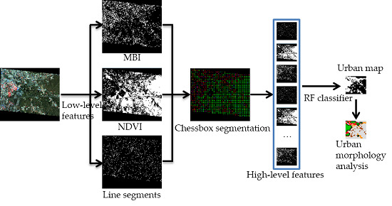
Therefore, in this study, a new approach is proposed to extract urban areas in high spatial resolution images. The flow chart of the proposed approach is shown in Figure 2. The primitive features reflecting the characteristics of buildings (building regions), vegetation, and line segments are first extracted.
In this study, the morphological building index (MBI) and the NDVI are used to represent the regional features of buildings and vegetation. However, the NDVI cannot always detect vegetation areas correctly, due to seasonal variations. The bare land is then mistakenly extracted as buildings, and is considered as an urban area. The line segments are used to solve this problem. The line segment characteristics of urban areas are significant, due to the dominant urban objects, such as buildings and roads, having regular shapes. Because it is quick and easy to implement, a chessboard segmentation algorithm is used to segment the entire image to obtain non-overlapping small spatial units. In each spatial unit, high-level features are abstracted from the MBI, the NDVI, and the line segment map. The random forest (RF) classifier is then employed for the classification of each spatial unit. Then, based on the spatial units, the spatial structure of the urban area is analyzed. The following sections describe the details.
3.1. Morphological Building Index (MBI)
The state-of-the-art MBI [37,38] building extraction method is used because it is free of parameters, multiscale, multidirectional, and unsupervised. The MBI has also been proved to be effective for automatic building extraction from high spatial resolution images [39,40]. The basic principle of the MBI is that buildings are brighter than their surroundings (especially building shadow). The MBI uses a set of morphological operators (e.g., top-hat by reconstruction, granulometry, and directionality) to represent the spectral–spatial regional properties of buildings (e.g., brightness, size, contrast, directionality, and shape). The calculation of the MBI is briefly described as follows.
Step 1: Brightness image. The maximum value for each pixel in the visible bands is kept as the brightness, since the visible bands make the most significant contribution to the spectral property of buildings.
Step 2: Top-hat morphological profiles. The differential morphological profiles of the top-hat transformation (DMPTH) represent the spectral–structural property of the buildings:
where TH represents the top-hat by reconstruction of the brightness image; s and d indicate the scale and direction of a linear structural element (SE), respectively; S and D represent the sets of scales and directions, respectively; and s is the interval of the profiles. The top-hat transformation can highlight the locally bright structures with a size up to a predefined value, and is used to measure the contrast.
Step 3: Calculation of the MBI. The MBI is defined by Equation (2):
where Nd and Ns are the number of directions and scales, respectively. The building index is defined as the average of the multiscale and multidirectional DMPTH, since building structures have larger feature values in most of the scales and directions in the morphological profiles, due to their local contrast and isotropy.
3.2. Normalized Difference Vegetation Index (NDVI)
The NDVI is used to represent the vegetation components, such as the grass and trees of urban areas, and farmland and forest in non-urban areas. Its calculation is based on the physical–chemical characteristic of vegetation, which has a strong reflectance in the NIR channel, but strong absorption in the red channel:
The vegetation map is obtained by applying Otsu thresholding [41] to the NDVI index.
3.3. Line Segments
The linear features are one of the most important characteristics of buildings, and are a good indicator of the existence of candidate buildings. Many studies have considered shadow as the proof of the existence of buildings [42,43]. Unfortunately, there are many factors that are beyond the control of the data user in very high resolution (VHR) satellite image acquisition, such as the sensor viewing angle, the solar angles, the season, the time, and the atmospheric conditions. Consequently, the shadow characteristics, such as size, shape, width, and length, are different in different images. Furthermore, in addition to buildings, many other objects, such as trees, vehicles, garden walls, pools, and bridges, cast shadows. Thus, the process of building shadow detection and extraction is time-consuming, and the accuracy of the results is not guaranteed.
Figure 3b shows the MBI and line segment features of Figure 3a. The line segments of the built-up areas are very different to those of the bare land. Because the bare land spectrum changes slowly, the MBI features of bare land are generally far away from the line segments. However, due to the relatively high luminance contrast between buildings and shadow, straight lines always appear on the sides of buildings in the immediate vicinity of shadow, as shown in Figure 3b. Such a line is called a dominant line (DL). In general, the length of the DL is similar to the length of the real building, and its inclination angle is also similar to the orientation of the real building.
In this study, the line segments are extracted by a fast, parameterless line segment detector named EDLines [44], based on the grayscale image. The grayscale image is obtained by forming a weighted sum of the R, G, and B bands of the original image (0.2989 × R + 0.5870 × G + 0.1140 × B [45]). The process consists of three steps: edge segment detection, line segment extraction, and line validation.
Step 1: Edge segments. Clean, contiguous chains of pixels are extracted by the edge drawing (ED) algorithm [46], based on the gradient magnitude and direction. The ED algorithm is very quick and accurate compared to the other existing edge detectors (e.g., Hough transform). The ED algorithm comprises four steps: denoising and smoothing of the images by a Gaussian filter, gradient magnitude and direction extraction for each pixel, detecting anchors which have the local maximum gradient values, and connecting anchors to obtain edge segments.
Step 2: Line segments. The least-squares line fitting method is used as the straightness criterion to extract line segments from the edge segments produced in the first step.
Step 3: Line validation. Line validation is adopted based on the Helmholtz principle to eliminate the false line segments.
Figure 3c–e shows an example of EDLines extraction. Figure 3d shows the ED results of Figure 3c, where the boundaries of the image are extracted. The boundaries of the interior of building objects are extracted, and the boundaries are not smooth and neat. Figure 3e shows the final result of the EDLines algorithm, where it can be seen that the line segments are much smoother than the edge segments (Figure 3d), and many of the trivial short boundaries are removed.
3.4. Chessboard Segmentation
Chessboard segmentation is the simplest segmentation method as it involves splitting the image into non-overlapping square objects with a size predefined by the user. Chessboard segmentation does not consider the underlying data (e.g., the MBI, the NDVI, and the line segment feature maps in this study) and, therefore, the features within the data are not delineated. This method is very suitable for segmenting complex urban areas.
3.5. High-Level Feature Extraction
High-level features reflecting the intrinsic characteristics of the urban areas are extracted from the primitive features for each spatial unit obtained by the chessboard segmentation. Figure 4 is the combination of the MBI, the NDVI, and the line segment feature maps of Figure 3a. The line segments of the built-up areas are very different to those of the bare land. Clearly, the MBI feature is the main factor to distinguish urban and non-urban areas. However, some bare soil is detected by the MBI, and some blue buildings are detected by both the MBI and the NDVI.
In each spatial unit, the high-level features of the three primitive feature maps of the MBI, the NDVI, and the line segments are extracted, respectively. In addition, the relationship between the MBI, the NDVI, and the line segments is also considered. In total, 24 high-level features are extracted from each spatial unit, as listed in Table 2.
For the MBI and the NDVI, the sum of the area percentage of the MBI and the NDVI is calculated. In general, water bodies, shadow, and some bare land (semi-arid and sub wetness land) belong to the black in Figure 4. Usually, in urban areas, buildings are distributed densely. Thus, in the MBI feature map, both the total and four quadrants of the area percentage are calculated. To distinguish the large and small areas of bare soil detected by the MBI, the number plot and area percentage of the MBI plot with different areas are calculated. The large-area MBI plot is larger than 500 pixels in this study, which is determined by the resolution of the images and the average areas of the buildings. In the NDVI feature map, the total area percentage is calculated. In general, urban area vegetation distribution is fragmented, and non-urban-area vegetation usually occurs in large-area blocks. Thus, the number and area percentage of the NDVI plot (area >500 pixels) are calculated.
In the line segment map, the number of line segments and the mean and variance of all the line segments lengths are calculated. It can be seen in Figure 3b and Figure 4 that the directional distribution of the line segments is significantly different between the urban and non-urban areas. In this study, the direction of the line segments is defined as 0–180° with a step of 30°, namely, six directions. The histogram is sorted in descending order according to the number of line segments. The direction with the maximum number of line segments, namely, the first direction, is called the dominant direction. Three features are extracted from the direction histogram of the line segments, namely, the percentage of dominant direction line segments (DLR), the angle difference between the top two dominant directions (difv), and the percentage of the top two dominant direction line segments.
Many bright non-building areas are detected as buildings by the MBI, especially the large areas of bare land and bare mountain, which seriously hinders the urban area extraction accuracy. Through observation of the experimental data, it can be seen that the spatial relationships between the MBI, the NDVI, and the line segments are different in different spatial contexts. In general, the MBI features of buildings overlap or are in close proximity to the line segments, due to the sudden significant spectral change between buildings and their surroundings (especially building shadow). However, the MBI features of bare land are generally far away from the line segments. This is because the bare land spectrum changes slowly (as shown in Figure 3b). Thus, the spatial relationships between the MBI, the NDVI, and the line segments are extracted in the neighborhood of the line segments, namely, the percentage of the MBI, the NDVI, and others (water, shadow, and so on) in the line segment buffer with a 1-pixel width.
The values of all the 24 features are greater than or equal to zero. The scales of all the features’ values are similar, i.e., 0–100, except for features 16, 17, 20, and 21.
3.6. Classification
High-dimensionality features extracted for recognizing urban areas are a binary classification problem. Hence, a nonparametric classifier is required, i.e., a classifier that does not assume any peculiar statistical distribution for the input. The classifier also has to be able to handle high-dimensional feature spaces, since the high-level features are composed of 24 bands. Although the high-dimensional features are artificially selected for the urban area extraction, they may contain redundancies in the feature space. It is also important to understand the importance of each feature. Therefore, the random forest (RF) classifier is used in this study for the urban area mapping, and to analyze the importance of each feature. The RF classifier can manage a high-dimensional feature space, and is both quick and robust [16].
The RF classifier constructs a multitude of decision trees, and is an approach that has been shown to perform very well [15,16]. A large number of trees (classifiers) are generated, and majority voting is finally used to assign an unknown model to a class. Each decision tree of RF chooses a subset of features randomly, and creates a classifier with a bootstrap sample from the original training samples. After the training, RF can assign a quality measure to each feature. In this study, the Gini index [12] is used as the feature selection measure in the decision tree design. The Gini index measures the impurity of a feature with respect to the classes:
where T represents the training set, and Ci represent a class. f(Ci, T)/|T| is the probability of the selected pixel belonging to class Ci.
At each node of the decision tree, the feature with the lowest Gini index value is selected from the randomly selected features as the best split, and is used to split the corresponding node. About one-third of the observed training samples (the “out-of-bag” samples) are not used when growing a tree, due to each tree of RF being grown from a bootstrapped sample. The variable importance is represented by the decrease in accuracy using the out-of-bag observations when permuting the values of the corresponding variables.
3.7. Morphological Spatial Pattern Analysis (MSPA)
Urban areas are created through urbanization and are categorized by urban morphology as cities, towns, conurbations, or suburbs. In general, conurbations and suburbs are interconnected with cities or towns, and the remote, sparse villages are not part of the urban areas. The RF classification map cannot clearly distinguish between villages and urban areas based on the local spatial and spectral information. Furthermore, some bare land with rich texture information can be misclassified as urban areas. MSPA [3,47,48] is therefore introduced to refine the urban map, and to further analyze the urban morphology.
In the binary or thresholded map (foreground and background), MSPA is used to analyze the shape, form, geometry, and connectivity of the map components. This consists of a series of sequential mathematical morphological operators such as erosion, geodesic dilation, reconstruction by dilation, and anchored skeletonisation. MSPA borrows the notion of path connectivity to determine the eight-connected or four-connected regions of the foreground. Each foreground pixel is classified as one of a mutually exclusive set of structural classes, i.e., Core, Islet, Edge, Loop, Perforation, Bridge, or Branch. In different applications, the corresponding objects in the generic MSPA categories are different [3,49]. There are two key parameters in MSPA, i.e., the foreground connectivity (FGconn) and the size parameter (Ew). Parameter Ew defines the width or thickness of the non-core classes in the pixels. In this study, FGconn is set to four-connected, and Ew is set to 1 pixel.
As shown in Figure 5, the urban map of the test image R2 (Figure 5a) is input into MSPA. All the pixels of urban areas are foreground, and the others are background. Figure 5b shows the MSPA result. The output classes of MSPA are as follows: Core, the interior of the urban areas, city or town, excluding the urban perimeter edge; Islet, disjoint cities or towns that are too small to contain Core, which are mainly sparse villages; Loop, connected at more than one end to the same Core area cities, which occurs due to a river or wide road splitting the city or town; Bridge, connected at more than one end to different Core areas; and Branch, connected at one end to Edge, Bridge, or Loop, and it shows the trail of the conurbations or suburbs that link the cities or towns. In this paper, for urban area extraction and urban morphology analysis, some of the Islets need to be abandoned. These Islets are mainly small villages far away from the city or built-up areas.
4. Experiments and Results
4.1. Experimental Design and Setup
The proposed method was validated on six complex and challenging high-resolution remote sensing images (as shown in Table 1 and Figure 1). In this section, the classification results of the proposed method are first compared with those of the other methods, namely, PanTex [10] and support vector machine (SVM) [50]. The sensitivity of the features and parameters of the proposed method is then analyzed. Finally, the spatial structure analysis of the urban areas is performed based on the urban area classification map.
The PanTex method is a robust built-up area presence index. The index is based on fuzzy rule-based composition of anisotropic textural co-occurrence measures derived from the satellite data by the GLCM [10]. Thus, in this study, the PanTex index is used as a comparison method for the urban area extraction. There are two parameters in PanTex: the window size (i.e., scale) and the threshold of the PanTex feature. The traditional PanTex method is a pixel-based method, and the PanTex feature of each pixel is extracted from the pixel-centered window. The threshold of the PanTex feature is then used to separate foreground (built-up areas or urban areas) and background (non-built-up areas or non-urban areas). All the test images in this study showed that the traditional PanTex method obtains very poor results, from both the visual effect and quantitative evaluation. Thus, in this experiment, the PanTex method was used as an object-based method, in order to obtain a fair comparison, and the window size was set as equal to the window size of the proposed method (i.e., 80–180, with a step size of 20). The threshold of PanTex was varied from the minimum to the maximum of PanTex, with a step size of 0.2. At each scale, the best PanTex result with the optimal threshold was selected for the comparison.
SVM is a widely used classification method for multi-dimensional datasets, and all 24 features were input into the SVM classifier in this study. The LIBSVM [50] toolbox was used, with a radial basis function (RBF) kernel. The LIBSVM toolbox has very sensitive parameters c and g. After several tests, the value of parameter g was varied from 7 × 10⁻⁸ to 9 × 10⁻⁵ with a step size of 2 × 10⁻⁸, and parameter c was varied from 0.5 to 15 with a step size of 0.5. The best result with the optimal parameter settings for c and g was selected to ensure a fair comparison.
The parameter settings in the experiments were as listed below.
- (1)
- MBI: Line-shaped SEs ranging from 2 to 32 with four directions.
- (2)
- NDVI threshold: The threshold of the NDVI was set according to the content of each image. The NDVI feature images were stretched to 0–255, and the NDVI thresholds of R1–R6 were set as 140, 150, 120, 155, 120, and 167, respectively.
- (3)
- Segmentation: Multiple scales of chessboard segmentation were tested in the experiments, from 80 to 180, with a step size of 20.
- (4)
- RF classification: Random forest was used for the feature selection and classification with 400 decision trees. RF was repeated nine times with different starting training samples, and the average accuracies are reported.
- (5)
- Accuracy assessment: The overall accuracy (OA) computed from the confusion matrix [51] was used to evaluate the classification accuracies. The accuracy assessment was performed on the original image sizes, and the numbers of ground-truth samples are listed in the fourth and fifth columns of Table 3.
Training: the classification training and testing was performed on the segmentation blocks. All of the pixels of one segmentation block have the same feature value, and the block number of each segmented image is small. Thus, the numbers of training samples are also small, as listed in Table 3.
In order to test and reduce the impact of the small numbers of training samples, three schemes of classifier training were tested:
- (1)
- Scheme 1: The training samples of each image were used to train one RF classifier.
- (2)
- Scheme 2: Training two RF classifiers for all the images. One classifier was obtained with the training samples of images R4 and R5, which feature barren vegetation. The other classifier was trained from all the training samples of images R1, R2, R3, and R6, which contain a lot of vegetation.
- (3)
- Scheme 3: Training one RF classifier for all six images. All the training samples of the six test images were used to train one RF classifier.
The above three schemes of classifier training were applied to the SVM classifier, and are denoted as SVM1, SVM2, and SVM3.
4.2. Comparison with Other Methods
Test R1: The classification accuracies of image R1 (WorldView-2 Harbin, Heilongjiang) based on the classification methods of PanTex, SVM, and the proposed method with the RF classifier are presented in Table 4. The classification maps of the RF1, PanTex, and SVM2 methods at scales of 80, 120, and 160 are displayed in Figure 6 to allow a visual comparison.
The RF1-based method shows an outstanding performance at all scales. The bottom left part of image R1 is bare land to be developed, and shows strong textural characteristics (as shown in Figure 1a), resulting in a relatively low OA (<91%) for PanTex in all the scales, as shown in Figure 6, second column. The OAs of RF1 are about 3–7% higher than those of PanTex at the same scale. At the same scale, the RF and SVM-based methods perform better than PanTex, except for RF3 at a scale of 80–100. It can be seen from Figure 6, third column, that many blocks in the middle of image R1 are labeled as non-urban areas by SVM.
Different training programs have a great impact on RF and SVM. The RF1 method shows the best performance (average OA = 94.3–95.7%), followed by RF2 (average OA = 92.3–94.9%), and finally RF3 (average OA = 86.5–92.2%). The RF1 and RF2 methods (average OA = 92.3–95.7%) are clearly better than RF3 (average OA = 86.5–92.2%). However, for the SVM-based methods, SVM2 is superior to SVM1 and SVM3. It can be seen from Table 4 that almost all the best accuracies of RF are superior to those of SVM in training schemes 1 and 2 at the same scale. The scale has a significant influence on image R1, and the optimal scale is different for the different methods. With the increase of the scale, the overall trend of the OA of RF2, RF3, SVM2, and SVM3 increases, while the trend of the OA of PanTex decreases.
Test R2: The classification accuracies of image R2 (WorldView-2, Harbin, Heilongjiang) based on the classification methods of PanTex, SVM, and the proposed method with the RF classifier are presented in Table 5. The classification maps of RF3, PanTex, and SVM3 at scales of 80,120, and 160 are displayed in Figure 7 for a visual comparison.
Almost all of the OAs of RF (average OAs of RF = 90.1–93.5%) and SVM (OAs of SVM1 and SVM2 = 91.3–94.1%) are higher than those of PanTex (OA = 88.5–91.4%) at the same scale, except for SVM1 (OA = 88.5–90.3%) and RF1 at a scale of 120. As shown in Figure 7, second column, the sparse vegetation covered fields are detected as urban areas by PanTex. Furthermore, the bright green grid-like vegetation area in the middle and lower right region of image R2 is also detected as urban area by PanTex. Thus, the OA of PanTex is relatively low at all scales. The scale has a regular impact on PanTex, i.e., the OA of PanTex decreases with the increase of the scale. However, for SVM and RF, the training programs have a greater impact than the scale. In addition, the different training programs have a greater impact on SVM than RF. The average OA differences between RF1 (90.1–92.6%, except for 89.0% at scale 120), RF2 (91.1–93.8%), and RF3 (91.5–93.5%) are small. The OA of SVM1 (88.5–90.3%) is lower than that of PanTex at the same scale. The OA of SVM2 (91.6–94.0%) shows a significant increase compared with SVM1. On the whole, SVM3 (OA = 91.3–94.1%) performs the best at all scales.
Test R3: The classification accuracies of image R3 (Gaofen-2, Guangzhou, Guangdong) based on the classification methods of PanTex, SVM, and the proposed method with the RF classifier are presented in Table 6. The classification maps of RF2, PanTex, and SVM2 at scales of 80, 120, and 160 are displayed in Figure 8 for a visual comparison.
It can be seen in Figure 1c that the upper right region of image R3 contains many small patches of dry soil, which show a strong texture characteristic when combined with the surrounding objects (buildings, roads, vegetation, etc.) In addition, the bottom right region contains a lot of scattered noise blocks covered with sparse vegetation. As shown in Figure 8, second column, the above two areas are detected as urban areas by PanTex, resulting in the low OA (87.8–88.0%) of PanTex at all scales. All the OAs of RF and SVM are higher than those of PanTex, and the RF performance is superior to SVM at the same scales, except for SVM1 at a scale of 80. Comparing images R1 and R2, it can be seen that the impact of the training programs in image R3 is smaller. The RF2 method (93.0–94.3%) shows the best performance, and the OA of RF2 is >5% higher than that of PanTex.
Test R4: The classification accuracies of image R4 (Gaofen-2, Guangzhou, Guangdong) based on the classification methods of PanTex, SVM, and the proposed method with the RF classifier are presented in Table 7. The classification maps of RF3, PanTex, and SVM3 at scales of 80, 120, and 160 are displayed in Figure 9 for a visual comparison.
As shown in Figure 1d, this image contains two types of bare land, namely, flat bare land (bottom left of R4) and bare mountain (right of R4), and both of these areas are large and have very little vegetation cover. PanTex (OA = 92.9–94.6%) shows a good performance in both types of bare land at small scales of 80–140, although the bare mountain areas contain distinctive texture features, as shown in Figure 9, second column, and Table 7. In general, the performance of RF (average OA = 90.3–93.6%) is better than SVM (OA = 87.5–93.6%). The training programs have less influence on RF than SVM. The differences in OA between the training programs are less than 1.6% at the same scale. The scale has a great influence on both RF and SVM, and RF3 (average OA = 93.1–93.6%) performs better than PanTex (OA = 92.9–93.4%) at large scales (e.g., 160–180). As shown in Figure 10c, these large areas of bare land are detected as buildings by the MBI due to the bright, dry soil. The distribution of the line segments and the MBI shows a distinct difference in Figure 10c,d. Although the line segment features can partially compensate for MBI’s erroneous detection, the performances of RF and SVM are still slightly degraded compared with PanTex at small scales (<160).
Test R5: The classification accuracies of image R5 (Gaofen-2, Guangzhou, Guangdong) based on the classification methods of PanTex, SVM, and the proposed method with the RF classifier are presented in Table 8. The classification maps of RF3, PanTex, and SVM3 at scales of 80, 120, and 160 are displayed in Figure 11 for a visual comparison.
There are large areas of bare land in this image, as shown in Figure 1e. The urban areas show distinctive texture characteristics compared with the bare land. PanTex makes a good distinction between the urban and non-urban areas, as shown in Table 8 and Figure 11, second column. PanTex obtains a higher OA than RF and SVM at all scales, except for the scale of 180. In addition, both the quantitative comparison and visual effect show that the scale has a relatively low impact for PanTex (OA = 93.3–95.0%).
The bare land contains many small, bright patches of dry soil, which are detected by the MBI as buildings, as shown in Figure 12b, thus degrading the performance of RF and SVM. However, with the increase of the scale, the adverse influence of the dry soil patches becomes smaller, as shown in Figure 11g,i (OA = 93.3% and 94.9%, respectively).
The OA differences between RF3 (SVM3) and PanTex become smaller (e.g., 4.4–1.8% (6.4–0.1%)). Furthermore, for RF and SVM, the influence of the scale is much greater than the influence of the training schemes. Overall, the OA of RF and SVM improves with the increase of the scale (e.g., the average OA of RF3 = 89.1–93.1% and the OA of SVM3 = 87.6–94.9%).
Test R6: The classification accuracies of image R6 (Gaofen-2, Guangzhou, Guangdong) based on the classification methods of PanTex, SVM, and the proposed method with the RF classifier are presented in Table 9. The classification maps of RF1, PanTex, and SVM2 at scales of 80, 120, and 160 are displayed in Figure 13 for a visual comparison.
This image is the most challenging test image. The image contains old city center, newly developed areas, areas to be developed, and open spaces. In the old city center, the buildings are very dense, small, and dark in color. As a result, its texture is not prominent. The surrounding newly developed areas contain relatively sparse, large, and bright buildings. The areas to be developed contain large areas of bare soil, very few buildings, and bright roads, as shown in the right bottom area of Figure 1f, which has obvious texture features. Meanwhile, the open spaces contain more types of land cover, e.g., small patches of bare soil, irregular paddy fields and farmland, and rivers and lakes. This type of area shows outstanding texture features. The above situation results in PanTex obtaining a relatively low OA (90.3–92.8%), as shown in Table 9 and Figure 13, second column.
Because this is the most challenging test image, the training scheme has a great influence, especially when the scale is relatively small. The results of RF are better than those of SVM at the same scale. RF1 obtains the best results (average OA = 93.4–95.2%), followed by RF2 (average OA = 92.5–94.8%), and finally RF3 (average OA = 89.2–94.1%). Among the SVM-based methods, SVM2 obtains the best results (maximum OA = 90.7–94.3%).
4.3. Parameter Sensitivity Analysis
From the accuracies of test images R1–R6, as shown in Table 4, Table 5, Table 6, Table 7, Table 8 and Table 9, the following conclusions can be drawn: Firstly, the training schemes have a significant impact on RF and SVM due to the fact that the test image size is limited, and thus the training samples are not sufficient, especially for a complex image. In all six test images, the scale has a greater influence than the training scheme. Secondly, the influence of scale for PanTex is less than for RF and SVM. The optimal scale is different for the different methods. The optimal scale for one image is affected by both the image resolution and the complexity of the image. For example, the optimal scales for PanTex are 80, 80, 140, 80, 140, and 80 for R1–R6, respectively; the optimal scales for RF2 are 160, 80, 160, 120, 180, and 180 for R1–R6, respectively; and the optimal scales for SVM2 are 180, 100, 120, 140, 180, and 180 for R1–R6, respectively.
The bars of Figure 14 represent the average (Ave) OA (%) of the test images at all scales obtained by the RF-based methods (RF1, RF2, and RF3), the SVM-based methods (SVM1, SVM2, and SVM3), and the PanTex (OA = 91.2%) method. The black and red lines are, respectively, the average and standard deviation (SD) of the OA (%) (denoted as OA Ave and OA SD) of RF1, RF2, RF3, PanTex, SVM1, SVM2, and SVM3 obtained from all the test images at all scales.
The black line in Figure 14 shows that RF has obvious overall advantages compared with PanTex and SVM, and RF2 obtains the best results (OA = 92.8%), followed by RF1 (OA = 92.6%) and RF3 (OA = 92.0%). The SVM1 OA (90.2%) is the most stable (SD = 0.9) and is also the lowest, followed by SVM3 (91.8%) and SVM2 (91.9%). It can be seen from the black line in Figure 14 that training scheme 2 achieves the best results for both RF and SVM. Training scheme 1 has a much smaller sample size than scheme 2, and SVM1 is not adequately trained, thereby obtaining the worst result. However, RF1 obtains a much better result, even when the sample size is very small, because RF has the ability to select features. It can be seen that when the training samples are sufficient and correct, the classifier can reach its potential [52]. Furthermore, the optimal value of the RF parameter can be easily found. However, the ranges of suitable values for parameters g and c of SVM are very difficult to determine.
It can be seen in Table 4, Table 5, Table 6, Table 7, Table 8 and Table 9 that, for the same test image, PanTex is less scale-sensitive than RF and SVM. However, Figure 14 indicates that the PanTex OA shows a very large fluctuation between the different images. Furthermore, the red line in Figure 14 clearly shows that the SD of PanTex is larger (SD = 2.4) than the SD of RF and SVM. Thus, it is concluded that PanTex is much more sensitive to the image content, and is not robust compared with RF and SVM.
4.4. Feature Analysis
In this study, 24 features are used, including the primary regional and line segment features, and advanced-level features, which reflect the spatial relationship of the primary-level features. In this section, the importance of each feature in the RF training is analyzed. Three training programs are observed and analyzed, as shown in Figure 15, Figure 16 and Figure 17. The height of the bars indicates the degree to which the accuracy or Gini coefficient decreases when this feature is not used. The upper bar graph is the mean decrease in accuracy over all classes; the lower bar graph is the mean decrease in Gini index.
Figure 15 shows the importance of the 24 features in each of the RF1 classifiers (one test image is training one RF1 classifier), training at a scale of 160. Clearly, the importance of each feature is very different for each image, as shown in Figure 15. Some features have a significant influence in some of the test images; for example, features 13 (A_NDVI) and 15 (the second feature of big_NDVI) in Figure 15a,b and features 16 (num_EDline), 18 (DLR), and 19 (DLR2) in Figure 15e. In general, features 2–7 (A_MBI, Qua_MBI, and num_MBI (area >500 pixels)) and 22–23 (the first two features of L_nb) play a significant role in improving the classification accuracy in all the test images, compared to the other features. However, some features have a negative impact on the classification accuracy; for example, features 16, 17, 19, and 20 in Figure 15c (the mean decreases in accuracy over all classes are −1.6 × 10⁻⁴%, −1.7 × 10⁻⁴%, −2.5 × 10⁻⁴%, and −7.2 × 10⁻⁴%).
Figure 16 shows the importance of the 24 features in each of the RF2 classifiers at scales of 80, 120, and 160, where one RF2 classifier is trained from test images R1, R2, R3, and R6, and another is trained from test images R4 and R5. In general, the feature importance for RF2 is consistent with RF1, i.e., features 2–7 and 22–23 play a significant role in improving the classification accuracy, as shown in Figure 16. In addition, at the different scales, the feature importance is similar for both RF2 classifiers. In Figure 16a–c, where the RF2 classifier is trained from test images R1, R2, R3, and R6, features 2–7, 10 (the first feature of area_MBI), 13 (A_NDVI), 15 (the second feature of big_NDVI), and 22–23 have a relatively large influence at all three scales (80, 120, and 160), compared with the other features. In Figure 16d–f, features 2–7, 16 (num_EDline), 18–19 (DLR and DLR2), and 22–23 have a relatively large influence at all three scales. However, several features play a very different role in the RF2 classifiers. For example, in the first row, features 13 and 15 have an obvious positive effect on the accuracy improvement compared with the second row. However, in the second row, features 16, 18, and 19 have an obvious positive effect on the accuracy improvement compared with the first row.
Figure 17 shows the importance of the 24 features in the RF3 classifiers (all six test images R1–R6 training one RF3 classifier), training at scales of 80, 120, and 160. At the different scales, the features that play a significant role in improving the RF3 classification accuracy are consistent, namely, features 2–7 and 22–23, as shown in Figure 17.
Overall, the importance of the basic features extracted from the line segments is not significant. However, all three training schemes for all the test images show that the neighborhood of the line segment features plays a significant positive role in improving the classification accuracy, i.e., the features extracted from the line segments play an important role.
4.5. Spatial Structure Analysis of Urban Areas
The urban morphology was also extracted and analyzed by MSPA using the best results of the RF-based method of each test image. MSPA was executed on the urban classification map, each pixel of which corresponds to a segment block of the original image. Thus, parameter Ew of MSPA was set to the smallest value, namely, 1 pixel. Figure 18, second column, shows the urban morphology categorized by MSPA. Each of the urban blocks extracted by the RF-based methods (the first column of Figure 18) is allocated to one of a mutually exclusive set of structural classes: Core, Islet, Loop, Bridge, Perforation, Edge, and Branch, where the category Edge is the edge of Core.
Test R1: Figure 18a was obtained by the RF-based method at a scale of 160, and Figure 18b is the corresponding MSPA category map. Clearly, Core is the largest area of the main city of this region. The newly developed area (on the left of R1) and the small town outside the main city (on the right of R1) are labeled as Branch, linked to the main city. The large areas of green space in the city (Core) are classified as Perforation, or are enclosed by Loop or Edge, as shown in Figure 18b. In this test image R1, the Islets are adjoined to the main city and are mainly the surrounding towns, so they are part of the urban area.
Test R2: Figure 18c was obtained by the RF-based method at a scale of 100, and Figure 18d is the corresponding MSPA category map. Clearly, the Cores are the regions of towns, which are split by roads and green areas (classified as Bridge). The small and scattered sparse villages or small towns, which are far away from the city (Core), are detected as Islets, as shown in Figure 1b. Thus, the Islets are not part of the urban area in test image R2, and can be removed based on their size and distance from the main city.
Test R3: Figure 18e was obtained by the RF-based method at a scale of 120, and Figure 18f is the corresponding MSPA category map. It can be seen from Figure 18f that the categories of Branch and Bridge account for a large proportion compared with the other test images. This is consistent with the visual interpretation of the original image. It can be seen from Figure 1c that the main old city is mainly distributed in the middle region of test image R3, and is labeled as Core. The main old city is surrounded by a wide range of new development zones, which are detected as small-area Core links with many branches, and the connection area is classified as Bridge. Some small-area built-up regions split by river or vegetation are classified as Islet.
Test R4: Figure 18g was obtained by the RF-based method at a scale of 160, and Figure 18h is the corresponding MSPA category map. Clearly, the main city features two large areas of Core. The surrounding towns are connected with the main city by roads (labeled as Bridge), and are labeled as Branch or Core (small area). Most of the Islets are the small towns outside the main city. However, the three Islets in the right middle of Figure 18h are a bare mountain area that has been misclassified as urban area. The misclassified Islets can be removed according their size (<2 pixels).
Test R5: Figure 18i was obtained by the RF-based method at a scale of 160, and Figure 18j is the corresponding MSPA category map. The building-intensive large area of the main city is classified as Core, and its surrounding conurbations or suburbs linked to the main city are labeled as Branch. The left part of test image R5 is mainly conurbations or suburbs, which contain relatively sparse buildings and several patches of bare soil. The Islets are small built-up regions not far from the main city, and are part of the urban area.
Test R6: Figure 18k was obtained by the RF-based method at a scale of 180, and Figure 18l is the corresponding MSPA category map. Large areas of connected built-up area are labeled as Core, and the surrounding towns are also labeled as small-area Core. Many of the smaller regions are labeled as Branch or Bridge. The Islets in test image R6 are part of the urban area, because they are relatively close to the city.
In general, the MSPA results are consistent with the visual interpretation. The urban morphology, i.e., the main cities, towns, conurbations, suburbs, and villages, are accurately distinguished by MSPA. In addition, according to the results of MSPA, the urban area mapping can be further refined. Except for a few small and long-distance Islets, all the remaining foreground areas are urban areas, i.e., Edge, Core, Loop, Branch, and Bridge.
5. Discussion
In this study, experiments were conducted with six very challenging images acquired by different satellites and different seasons. According to the results of the experiments, the following conclusions can be made:
(1) The low-level primitive features used are the MBI, the NDVI, and line segments. The MBI and the NDVI are efficient proxies of regional features of buildings and vegetation, and the line segments are very different between urban and non-urban areas.
(2) The fast chessboard segmentation method is used to split the image into non-overlapping square objects, and does not consider the underlying data. This approach is very suitable for segmenting complex urban areas.
(3) The high-level feature extraction is conducted in the segmented square objects. The results of the experiments proved that the advanced features are well described and can reflect the characteristics of urban and non-urban areas. The feature analysis experiments with all six test images showed that the spatial relationship between the MBI, the NDVI, and the neighborhood of the line segments has a great effect on the improvement of the classification accuracy.
(4) The proposed urban area extraction framework was compared with the state-of-the-art PanTex method. The proposed framework was also tested using SVM methods. The experiments proved that the proposed urban area extraction framework is much more robust than PanTex. In general, both the RF- and SVM-based methods can obtain much higher OAs than PanTex, especially when the image is complex and challenging. However, PanTex can obtain better results when the image is simple and the scale is smaller. Overall, the RF-based method performs better than the SVM-based method. Furthermore, the optimal value of the RF parameter is much easier to find than those of SVM. In addition, the training schemes proved that when the training samples are sufficient and accurate, RF and SVM can reach their full potential. This study also proved that the number and abstraction level of the features play a very important role for object recognition, which will be further studied in our follow-up research.
(5) The urban morphology is well recognized, and is consistent with the visual interpretation. In this study, the MSPA was proven to be a very effective tool for the analysis of urban morphology at a macroscopic spatial extent.
6. Conclusions
In this study, a new object-oriented approach based on the fusion of regional and line segment features has been proposed for urban area extraction from high spatial resolution remote sensing images, and then urban morphology analysis. The proposed workflow incorporates two levels of spatial information, i.e., microscopic (local spatial units) and macroscopic spatial extents. After primitive feature extraction and segmentation, the urban area characteristics are described by the high-level features extracted from the low-level regional and line segment features in the local spatial units. Subsequently, RF is used for urban area extraction and feature analysis. Finally, MSPA is used at a macroscopic spatial extent to analyze the urban area morphology and refine the urban mapping results.
According to the experimental results, the urban area extraction method proposed effectively overcomes the difficult problem of distinguishing urban area from bare land, and is more robust than the state-of-the-art PanTex method, especially when the image is complex and challenging. In this study, the line features played a very positive role, especially the spatial relationship features between line segments and the MBI and the NDVI. This will be further studied in our follow-up research. Although 24 high-level features were extracted and analyzed in this study, the results proved that the number and abstraction level of the features play a very important role for urban area object recognition [35,36], which will also be further studied in our follow-up research. Meanwhile, the urban morphology reflects the macroscopic characteristic of the urban areas [53,54]. Thus, our future work will also focus on urban morphology analysis.
Acknowledgments
This work was supported in part by the National Natural Science Foundation of China under grants 41301472, and 61372147; the China National Science Fund for Excellent Young Scholars under grant 41522110; and the Foundation for the Author of National Excellent Doctoral Dissertation of China under grant 201348.
Author Contributions
Qian Zhang designed the proposed model, implemented the experiments, and drafted the manuscript. Xin Huang and Guixu Zhang provided overall guidance to the project, and reviewed and edited the manuscript.
Conflicts of Interest
The authors declare no conflict of interest.
References
- Tang, Y.; Zhang, L. Urban change analysis with multi-sensor multispectral imagery. Remote Sens. 2017, 9, 252. [Google Scholar] [CrossRef]
- Trianni, G.; Lisini, G.; Angiuli, E.; Moreno, E.; Dondi, P.; Gaggia, A.; Gamba, P. Scaling up to national/regional urban extent mapping using Landsat data. IEEE J. Sel. Top. Appl. Earth Obs. Remote Sens. 2015, 8, 3710–3719. [Google Scholar] [CrossRef]
- Suarez-Rubio, M.; Lookingbill, T.R.; Elmore, A.J. Exurban development derived from landsat from 1986 to 2009 surrounding the district of Columbia, USA. Remote Sens. Environ. 2012, 124, 360–370. [Google Scholar] [CrossRef]
- Ferreira, R.S.; Bentes, C.; Costa, G.A.; Oliveira, D.A.; Happ, P.N.; Feitosa, R.Q.; Gamba, P. A set of methods to support object-based distributed analysis of large volumes of earth observation data. IEEE J. Sel. Top. Appl. Earth Obs. Remote Sens. 2017, 10, 681–690. [Google Scholar] [CrossRef]
- Salentinig, A.; Gamba, P. A general framework for urban area extraction exploiting multiresolution sar data fusion. IEEE J. Sel. Top. App. Earth Obs. Remote Sens. 2016, 9, 2009–2018. [Google Scholar] [CrossRef]
- Tuia, D.; Camps-Valls, G. Urban image classification with semisupervised multiscale cluster kernels. IEEE J. Sel. Top. App. Earth Obs. Remote Sens. 2011, 4, 65–74. [Google Scholar] [CrossRef]
- Esch, T.; Thiel, M.; Schenk, A.; Roth, A.; Muller, A.; Dech, S. Delineation of urban footprints from TerraSAR-X data by analyzing speckle characteristics and intensity information. IEEE Trans. Geosci. Remote Sens. 2010, 48, 905–916. [Google Scholar] [CrossRef]
- Dell’Acqua, F.; Gamba, P. Texture-based characterization of urban environments on satellite SAR images. IEEE Trans. Geosci. Remote Sens. 2003, 41, 153–159. [Google Scholar] [CrossRef]
- Sun, G.; Chen, X.; Jia, X.; Yao, Y.; Wang, Z. Combinational build-up index (CBI) for effective impervious surface mapping in urban areas. IEEE J. Sel. Top. Appl. Earth Obs. Remote Sens. 2016, 9, 2081–2092. [Google Scholar] [CrossRef]
- Pesaresi, M.; Gerhardinger, A.; Kayitakire, F. A robust built-up area presence index by anisotropic rotation-invariant textural measure. IEEE J. Sel. Top. Appl. Earth Obs. Remote Sens. 2008, 1, 180–192. [Google Scholar] [CrossRef]
- Schneider, A.; Friedl, M.A.; Potere, D. A new map of global urban extent from MODIS satellite data. Environ. Res. Lett. 2009, 4, 044003. [Google Scholar] [CrossRef]
- Sophie, B.; Pierre, D.; Martin, H.; Lammert, K.; Vasileios, K.; Olivier, A. Producing global land cover maps consistent over time to respond the needs of the climate modelling community. In Proceedings of the International Workshop on the Analysis of Multi-Temporal Remote Sensing Images, Trento, Italy, 12–14 July 2011; pp. 161–164. [Google Scholar]
- Dennison, P.E.; Roberts, D.A. Endmember selection for multiple endmember spectral mixture analysis using endmember average RMSE. Remote Sens. Environ. 2003, 87, 123–135. [Google Scholar] [CrossRef]
- Hu, X.; Weng, Q. Estimating impervious surfaces from medium spatial resolution imagery using the self-organizing map and multi-layer perceptron neural networks. Remote Sens. Environ. 2009, 113, 2089–2102. [Google Scholar] [CrossRef]
- Pal, M. Random forest classifier for remote sensing classification. Int. J. Remote Sens. 2005, 26, 217–222. [Google Scholar] [CrossRef]
- Gislason, P.O.; Benediktsson, J.A.; Sveinsson, J.R. Random forests for land cover classification. Pattern Recognit. Lett. 2006, 27, 294–300. [Google Scholar] [CrossRef]
- Xia, J.; Liao, W.; Chanussot, J.; Du, P.; Song, G.; Philips, W. Improving random forest with ensemble of features and semisupervised feature extraction. IEEE Geosci. Remote Sens. Lett. 2015, 12, 1471–1475. [Google Scholar]
- Kawamura, M.; Jayamana, S.; Tsujiko, Y. Relation between social and environmental conditions in Colombo Sri Lanka and the urban index estimated by satellite remote sensing data. Int. Arch. Photogramm. Remote Sens. 1996, 31, 321–326. [Google Scholar]
- Zha, Y.; Gao, J.; Ni, S. Use of normalized difference built-up index in automatically mapping urban areas from tm imagery. Int. J. Remote Sen. 2003, 24, 583–594. [Google Scholar] [CrossRef]
- Xu, H. Analysis of impervious surface and its impact on urban heat environment using the normalized difference impervious surface index (NDISI). Photogramm. Eng. Remote Sens. 2010, 76, 557–565. [Google Scholar] [CrossRef]
- As-Syakur, A.R.; Adnyana, I.; Arthana, I.W.; Nuarsa, I.W. Enhanced built-up and bareness index (EBBI) for mapping built-up and bare land in an urban area. Remote Sens. 2012, 4, 2957–2970. [Google Scholar] [CrossRef]
- Amitrano, D.; Belfiore, V.; Cecinati, F.; Di Martino, G.; Iodice, A.; Mathieu, P.-P.; Medagli, S.; Poreh, D.; Riccio, D.; Ruello, G. Urban areas enhancement in multitemporal sar rgb images using adaptive coherence window and texture information. IEEE J. Sel. Top. Appl. Earth Obs. Remote Sens. 2016, 9, 3740–3752. [Google Scholar] [CrossRef]
- Tuia, D.; Volpi, M.; Dalla Mura, M.; Rakotomamonjy, A.; Flamary, R. Automatic feature learning for spatio-spectral image classification with sparse SVM. IEEE Trans. Geosci. Remote Sens. 2014, 52, 6062–6074. [Google Scholar] [CrossRef]
- Ghamisi, P.; Benediktsson, J.A.; Cavallaro, G.; Plaza, A. Automatic framework for spectral–spatial classification based on supervised feature extraction and morphological attribute profiles. IEEE J. Sel. Top. Appl. Earth Obs. Remote Sens. 2014, 7, 2147–2160. [Google Scholar] [CrossRef]
- Liao, W.; Bellens, R.; Pizurica, A.; Philips, W.; Pi, Y. Classification of hyperspectral data over urban areas using directional morphological profiles and semi-supervised feature extraction. IEEE J. Sel. Top. Appl. Earth Obs. Remote Sens. 2012, 5, 1177–1190. [Google Scholar] [CrossRef]
- Smits, P.C.; Annoni, A. Updating land-cover maps by using texture information from very high-resolution space-borne imagery. IEEE Trans. Geosci. Remote Sens. 1999, 37, 1244–1254. [Google Scholar] [CrossRef]
- Shackelford, A.K.; Davis, C.H. A hierarchical fuzzy classification approach for high-resolution multispectral data over urban areas. IEEE Trans. Geosci. Remote Sens. 2003, 41, 1920–1932. [Google Scholar] [CrossRef]
- Li, J.; Narayanan, R.M. Integrated spectral and spatial information mining in remote sensing imagery. IEEE Trans. Geosci. Remote Sens. 2004, 42, 673–685. [Google Scholar] [CrossRef]
- Huang, X.; Han, X.; Zhang, L.; Gong, J.; Liao, W.; Benediktsson, J.A. Generalized differential morphological profiles for remote sensing image classification. IEEE J. Sel. Top. Appl. Earth Obs. Remote Sens. 2016, 9, 1736–1751. [Google Scholar] [CrossRef]
- Weeks, J.R. Defining Urban Areas. In Remote Sensing of Urban and Suburban Areas; Springer, Inc.: New York, NY, USA, 2010; pp. 33–45. [Google Scholar]
- Huang, X.; Li, Q.; Liu, H.; Li, J. Assessing and improving the accuracy of GlobeLand30 data for urban area delineation by combining multisource remote sensing data. IEEE Geosci. Remote Sens. Lett. 2016, 13, 1860–1864. [Google Scholar] [CrossRef]
- Wilkinson, G.G. Results and implications of a study of fifteen years of satellite image classification experiments. IEEE Trans. Geosci. Remote Sens. 2005, 43, 433–440. [Google Scholar] [CrossRef]
- Li, C.; Wang, J.; Wang, L.; Hu, L.; Gong, P. Comparison of classification algorithms and training sample sizes in urban land classification with Landsat thematic mapper imagery. Remote Sens. 2014, 6, 964–983. [Google Scholar] [CrossRef]
- Gong, P.; Yu, L.; Li, C.; Wang, J.; Liang, L.; Li, X.; Ji, L.; Bai, Y.; Cheng, Y.; Zhu, Z. A new research paradigm for global land cover mapping. Ann. GIS 2016, 22, 87–102. [Google Scholar] [CrossRef]
- LeCun, Y.; Bengio, Y.; Hinton, G. Deep learning. Nature 2015, 521, 436–444. [Google Scholar] [CrossRef] [PubMed]
- Girshick, R.; Donahue, J.; Darrell, T.; Malik, J. Rich feature hierarchies for accurate object detection and semantic segmentation. In Proceedings of the IEEE Conference on Computer Vision and Pattern Recognition, Columbus, OH, USA, 23–28 June 2014; pp. 580–587. [Google Scholar]
- Huang, X.; Zhang, L. A multidirectional and multiscale morphological index for automatic building extraction from multispectral GeoEye-1 imagery. Photogramm. Eng. Remote Sens. 2011, 77, 721–732. [Google Scholar] [CrossRef]
- Huang, X.; Zhang, L. Morphological building/shadow index for building extraction from high-resolution imagery over urban areas. IEEE J. Sel. Top. Appl. Earth Obs. Remote Sens. 2012, 5, 161–172. [Google Scholar] [CrossRef]
- Huang, X.; Lu, Q.; Zhang, L. A multi-index learning approach for classification of high-resolution remotely sensed images over urban areas. Int. J. Photogramm. Remote Sens. 2014, 90, 36–48. [Google Scholar] [CrossRef]
- Zhang, Q.; Huang, X.; Zhang, G. A morphological building detection framework for high-resolution optical imagery over urban areas. IEEE Geosci. Remote Sens. Lett. 2016, 13, 1388–1392. [Google Scholar] [CrossRef]
- Otsu, N. A threshold selection method from gray-level histograms. IEEE Trans. Syst. Man Cybern. 1979, 9, 62–66. [Google Scholar] [CrossRef]
- Ok, A.O.; Senaras, C.; Yuksel, B. Automated detection of arbitrarily shaped buildings in complex environments from monocular vhr optical satellite imagery. IEEE Trans. Geosci. Remote Sens. 2013, 51, 1701–1717. [Google Scholar] [CrossRef]
- Ok, A.O. Automated detection of buildings from single vhr multispectral images using shadow information and graph cuts. Int. J. Photogramm. Remote Sens. 2013, 86, 21–40. [Google Scholar] [CrossRef]
- Akinlar, C.; Topal, C. Edlines: A real-time line segment detector with a false detection control. Pattern Recognit. Lett. 2011, 32, 1633–1642. [Google Scholar] [CrossRef]
- Kalaivani, K.; Praveena, R.; Anjalipriya, V.; Srimeena, R. Real time implementation of image recognition and text to speech conversion. Int. J. Adv. Res. Technol. 2014, 2, 171–175. [Google Scholar]
- Topal, C.; Akınlar, C.; Genç, Y. Edge drawing: A heuristic approach to robust real-time edge detection. In Proceedings of the International Conference on Pattern Recognition, Istanbul, Turkey, 23–26 August 2010; pp. 2424–2427. [Google Scholar]
- Vogt, P.; Riitters, K.H.; Estreguil, C.; Kozak, J.; Wade, T.G.; Wickham, J.D. Mapping spatial patterns with morphological image processing. Landsc. Ecol. 2007, 22, 171–177. [Google Scholar] [CrossRef]
- Soille, P. Morphological Image Analysis: Principles and Applications; Springer Science & Business Media: Berlin, Germany, 2013. [Google Scholar]
- Vogt, P.; Ferrari, J.R.; Lookingbill, T.R.; Gardner, R.H.; Riitters, K.H.; Ostapowicz, K. Mapping functional connectivity. Ecol. Indic. 2009, 9, 64–71. [Google Scholar] [CrossRef]
- Chang, C.-C.; Lin, C.-J. Libsvm: A library for support vector machines. ACM Trans. Intell. Syst. Technol. 2011, 2, 27. [Google Scholar] [CrossRef]
- Congalton, R.G.; Green, K. Assessing the Accuracy of Remotely Sensed Data: Principles and Practices, 2nd ed.; CRC Press: London, UK, 2008; pp. 55–61. [Google Scholar]
- Tuia, D.; Persello, C.; Bruzzone, L. Domain adaptation for the classification of remote sensing data: An overview of recent advances. IEEE Geosci. Remote Sens. Mag. 2016, 4, 41–57. [Google Scholar] [CrossRef]
- Huang, X.; Wen, D.; Li, J.; Qin, R. Multi-level monitoring of subtle urban changes for the megacities of china using high-resolution multi-view satellite imagery. Remote Sens. Environ. 2017, 196, 56–75. [Google Scholar] [CrossRef]
- Montanges, A.P.; Moser, G.; Taubenböck, H.; Wurm, M.; Tuia, D. Classification of Urban Structural Types with Multisource Data and Structured Models. In Proceedings of the 2015 Joint Urban Remote Sensing Event (JURSE), Lausanne, Switzerland, 30 March–1 April 2015. [Google Scholar]
Figure 1.
The six test images: (a–f) R1–R6, respectively.
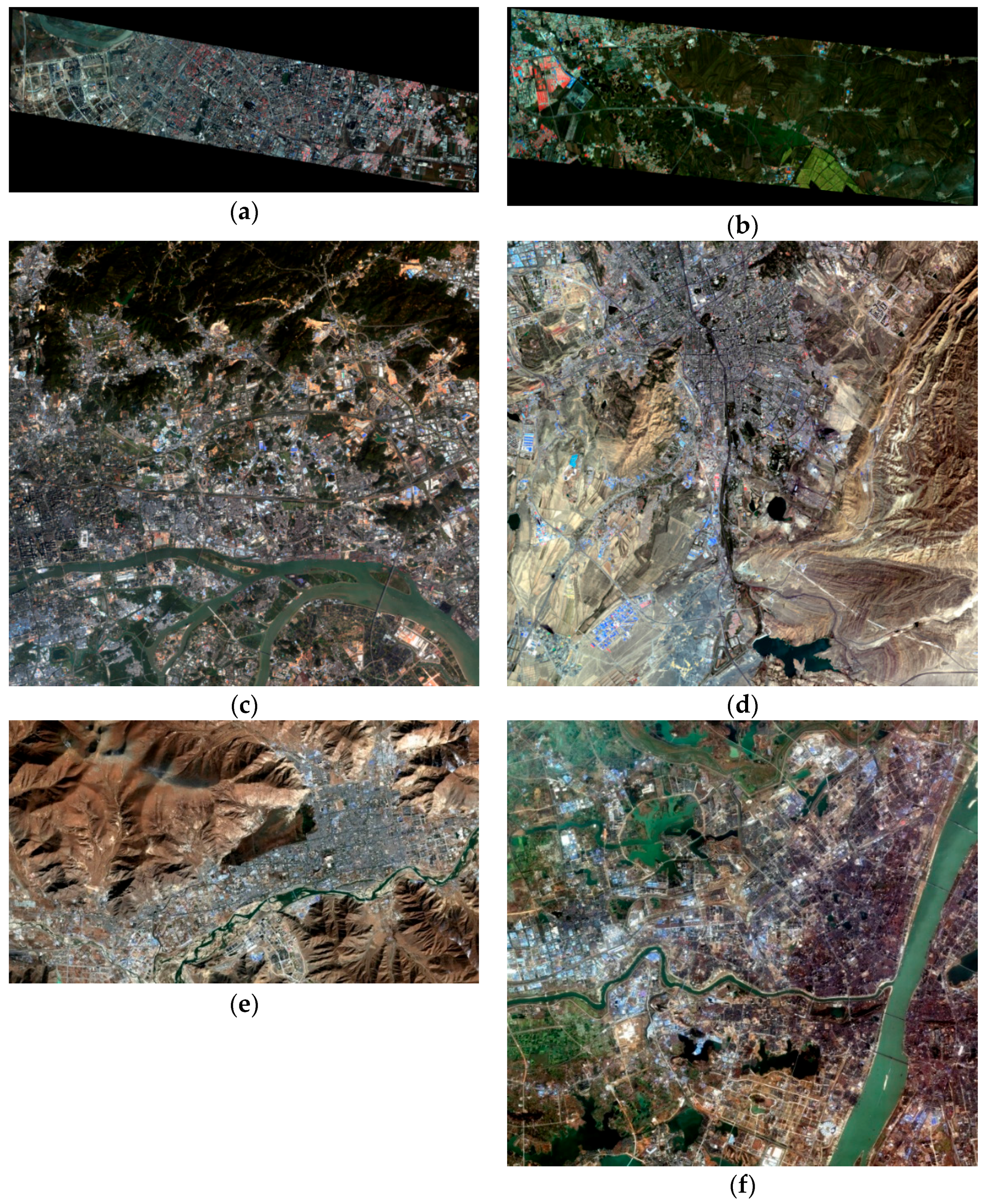
Figure 2.
General workflow of this study.

Figure 3.
(a) The R, G, and B bands of the original image; (b) the MBI (red) and line segment (cyan) feature map of (a); (c) a subset of (a); and (d,e) the edge drawing and line segments results of (c).
Figure 3.
(a) The R, G, and B bands of the original image; (b) the MBI (red) and line segment (cyan) feature map of (a); (c) a subset of (a); and (d,e) the edge drawing and line segments results of (c).

Figure 4.
The MBI, the NDVI, and the line segment feature map of Figure 3a (red color: MBI, green color: NDVI, blue color: line segments). The blue and yellow rectangles frame the MBI and NDVI mis-extraction.
Figure 4.
The MBI, the NDVI, and the line segment feature map of Figure 3a (red color: MBI, green color: NDVI, blue color: line segments). The blue and yellow rectangles frame the MBI and NDVI mis-extraction.

Figure 5.
(a) Urban classification map of test image R2 as the MSPA input (White: foreground; black: background); and (b) MSPA results.
Figure 5.
(a) Urban classification map of test image R2 as the MSPA input (White: foreground; black: background); and (b) MSPA results.
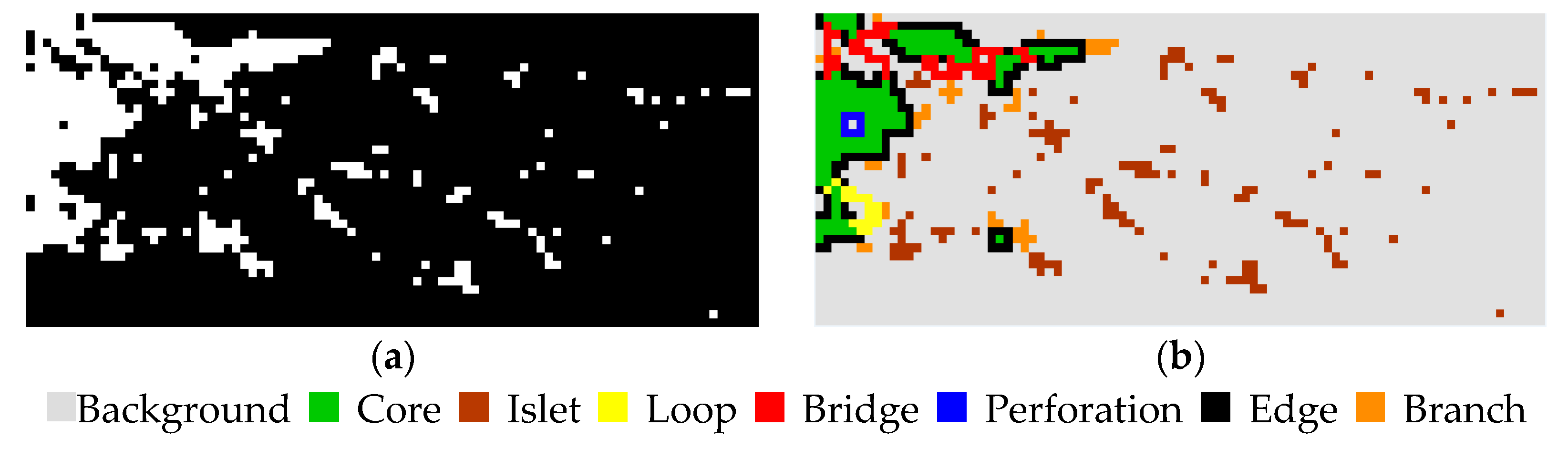
Figure 6.
(a–i) The urban area classification maps for the R1 image with scales of 80, 120, and 160, shown in rows 1, 2, and 3, respectively. Columns 1 to 3 are the results of the RF1, PanTex, and SVM2 methods, respectively.
Figure 6.
(a–i) The urban area classification maps for the R1 image with scales of 80, 120, and 160, shown in rows 1, 2, and 3, respectively. Columns 1 to 3 are the results of the RF1, PanTex, and SVM2 methods, respectively.

Figure 7.
(a–i) The urban area classification maps for the R2 image with scales of 80, 120, and 160, shown in rows 1, 2, and 3, respectively. Columns 1–3 are the results of the RF3, PanTex, and SVM3 methods, respectively.
Figure 7.
(a–i) The urban area classification maps for the R2 image with scales of 80, 120, and 160, shown in rows 1, 2, and 3, respectively. Columns 1–3 are the results of the RF3, PanTex, and SVM3 methods, respectively.
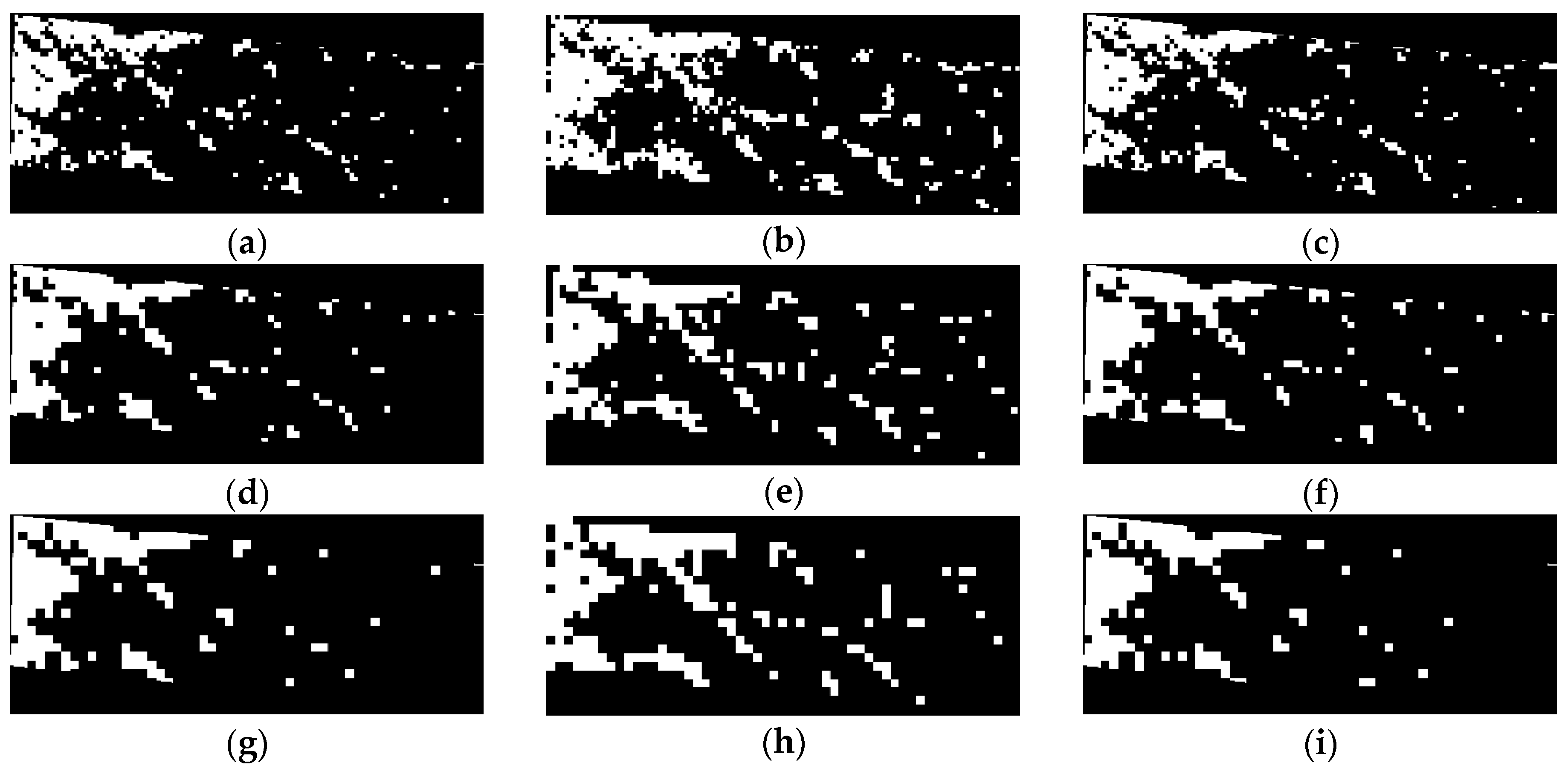
Figure 8.
(a–i) The urban area classification maps for the R3 image with scales of 80, 120, and 160, shown in rows 1, 2, and 3, respectively. Columns 1–3 are the results of the RF2, PanTex, and SVM2 methods, respectively.
Figure 8.
(a–i) The urban area classification maps for the R3 image with scales of 80, 120, and 160, shown in rows 1, 2, and 3, respectively. Columns 1–3 are the results of the RF2, PanTex, and SVM2 methods, respectively.

Figure 9.
(a–i) The urban area classification maps for the R4 image with scales of 80, 120, and 160, shown in rows 1, 2, and 3, respectively. Columns 1–3 are the results of the RF3, PanTex, and SVM3 methods, respectively.
Figure 9.
(a–i) The urban area classification maps for the R4 image with scales of 80, 120, and 160, shown in rows 1, 2, and 3, respectively. Columns 1–3 are the results of the RF3, PanTex, and SVM3 methods, respectively.

Figure 10.
(a,b) Two subsets of R4; and (c,d) their corresponding MBI (red) and line segment (cyan) feature maps.
Figure 10.
(a,b) Two subsets of R4; and (c,d) their corresponding MBI (red) and line segment (cyan) feature maps.
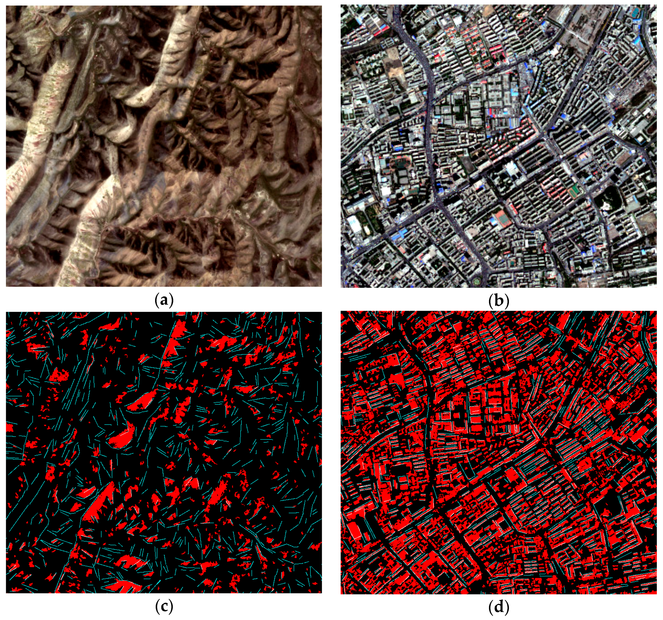
Figure 11.
(a–i) The urban area classification maps for the R5 image with scales of 80, 120, and 160, shown in rows 1, 2, and 3, respectively. Columns 1–3 are the results of the RF3, PanTex, and SVM3 methods, respectively.
Figure 11.
(a–i) The urban area classification maps for the R5 image with scales of 80, 120, and 160, shown in rows 1, 2, and 3, respectively. Columns 1–3 are the results of the RF3, PanTex, and SVM3 methods, respectively.

Figure 12.
(a) A subset of R5; and (b) the MBI (red) and line segment (cyan) feature maps of (a).

Figure 13.
(a–i) The urban area classification maps for the R6 image with scales of 80, 120, and 160, shown in rows 1, 2, and 3, respectively. Columns 1–3 are the results of the RF1, PanTex, and SVM2 methods, respectively.
Figure 13.
(a–i) The urban area classification maps for the R6 image with scales of 80, 120, and 160, shown in rows 1, 2, and 3, respectively. Columns 1–3 are the results of the RF1, PanTex, and SVM2 methods, respectively.
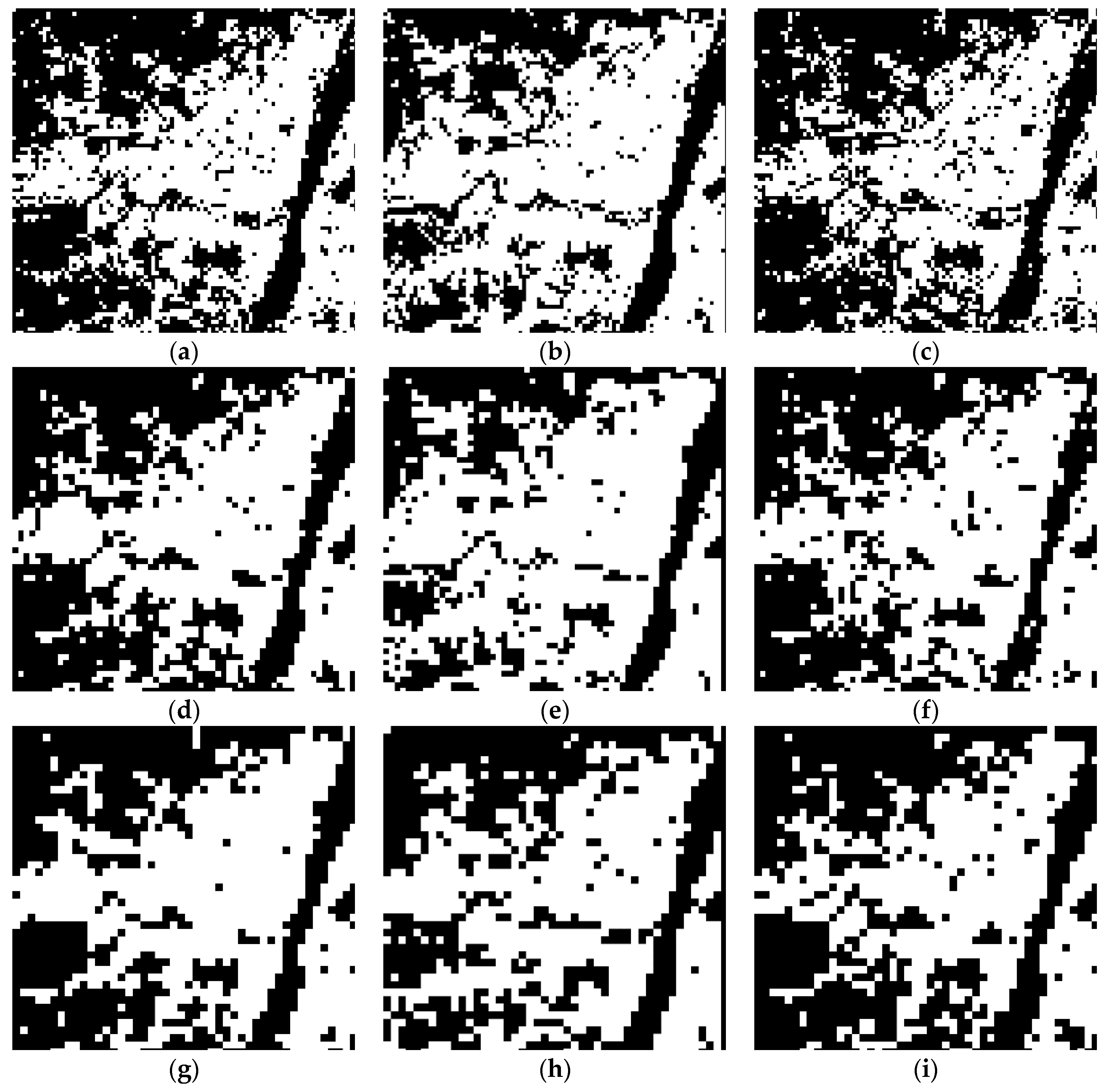
Figure 14.
The left vertical axis is the OA (%), and the right is the standard deviation (SD) of the OA. The bars represent the average (Ave) OA (%) of test images R1–R6 at all scales. The black and red lines are, respectively, the average and SD OA of all the test images at all scales for the RF1, RF2, RF3, PanTex, SVM1, SVM2, and SVM3 methods.

Figure 15.
The importance of the 24 features in each of the RF1 classifiers, training at a scale of 160. Each test image is trained for one RF1 classifier (a–f).
Figure 15.
The importance of the 24 features in each of the RF1 classifiers, training at a scale of 160. Each test image is trained for one RF1 classifier (a–f).
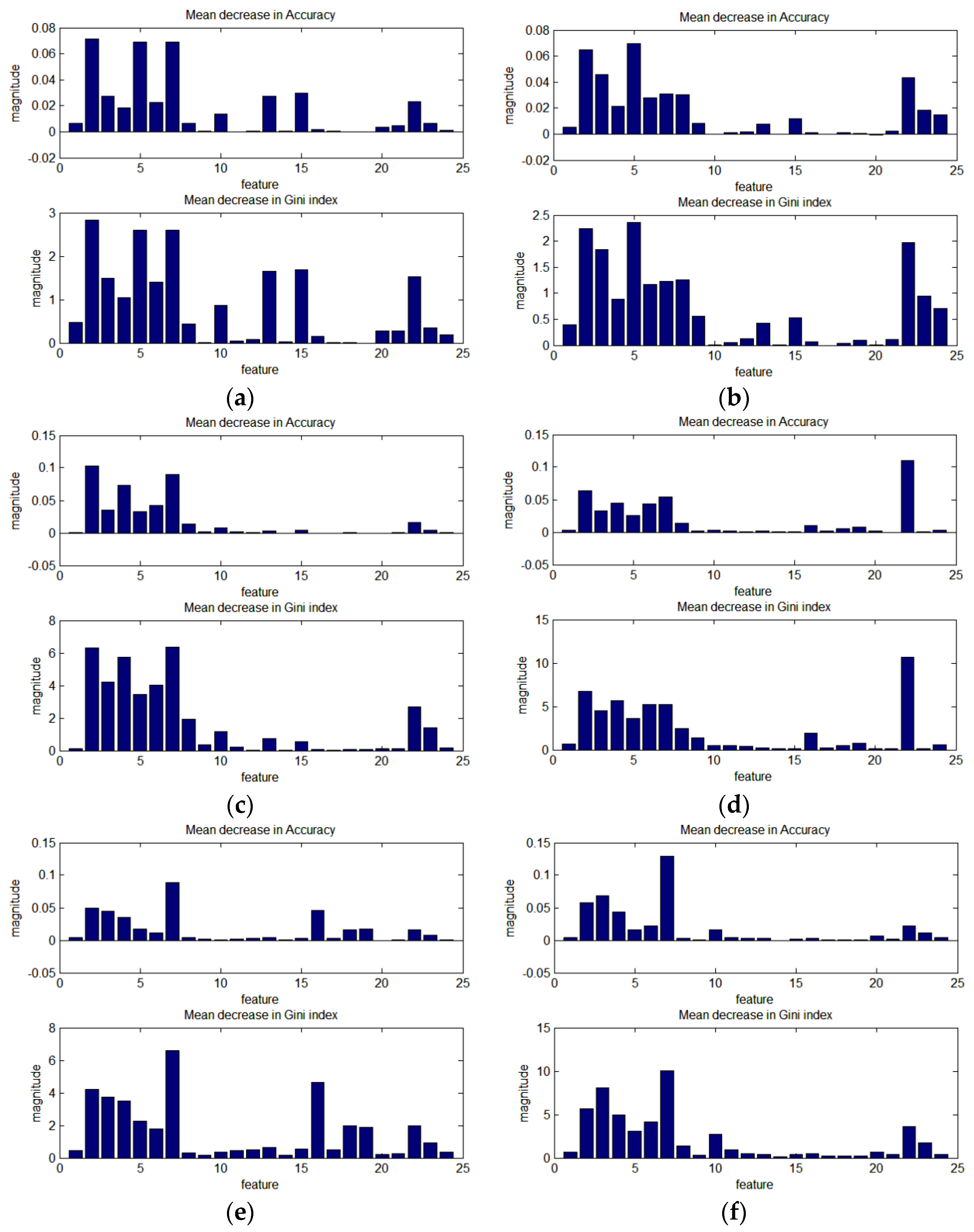
Figure 16.
(a–f) The importance of the 24 features in each of the RF2 classifiers at scales of 80 (first row), 120 (second row), and 160 (third row). First column: One RF2 classifier is trained from test images R1, R2, R3, and R6. Second column: Another RF2 classifier is trained from test images R4 and R5.

Figure 17.
The importance of the 24 features in the RF3 classifiers, training at scales of: 80 (a); 120 (b); and 160 (c).
Figure 17.
The importance of the 24 features in the RF3 classifiers, training at scales of: 80 (a); 120 (b); and 160 (c).

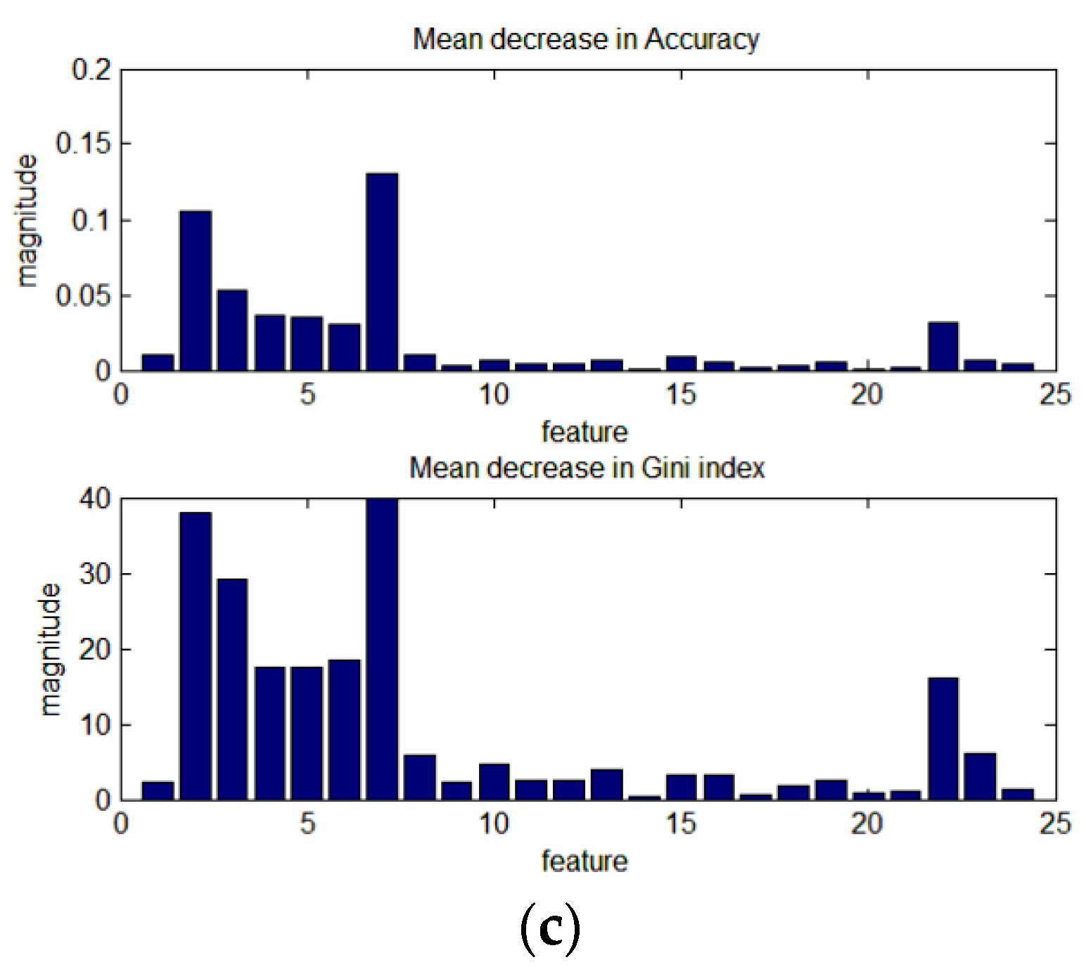
Figure 18.
(a–l) The urban morphology spatial pattern analysis (the second column) of the urban area classification maps (the first column) for test images R1–R6.
Figure 18.
(a–l) The urban morphology spatial pattern analysis (the second column) of the urban area classification maps (the first column) for test images R1–R6.


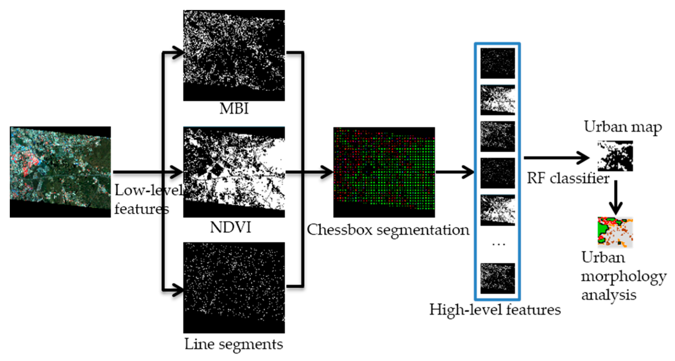
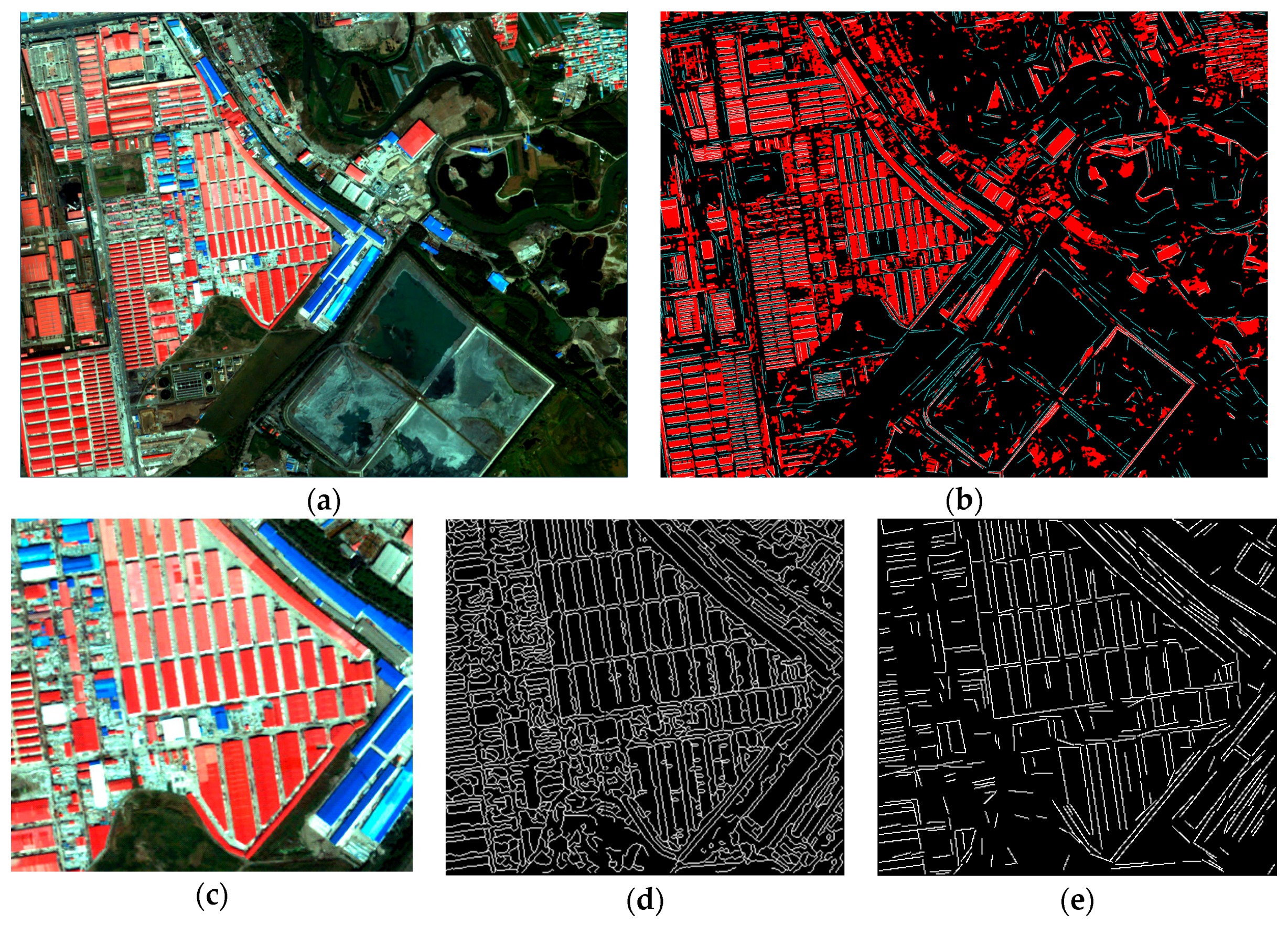
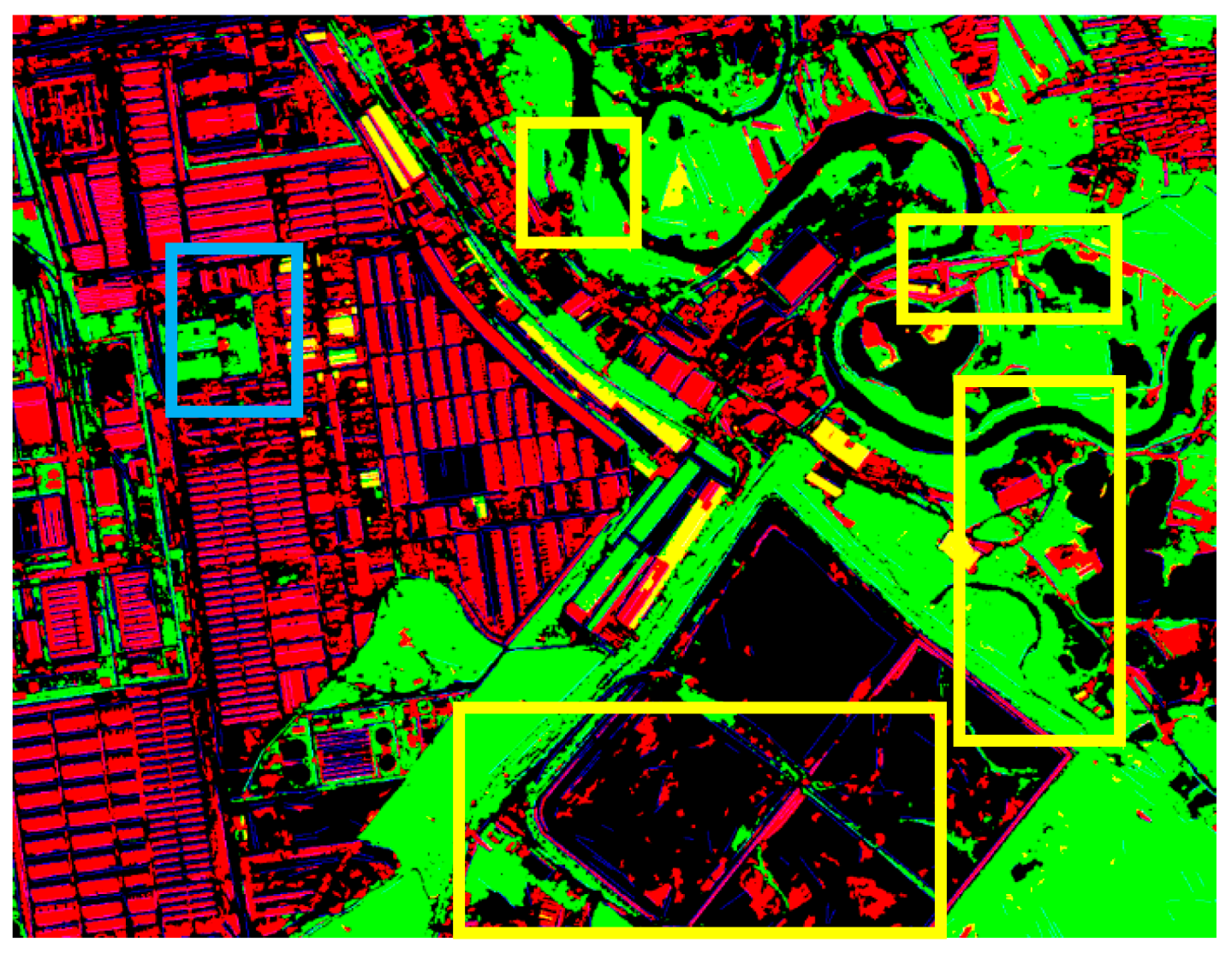
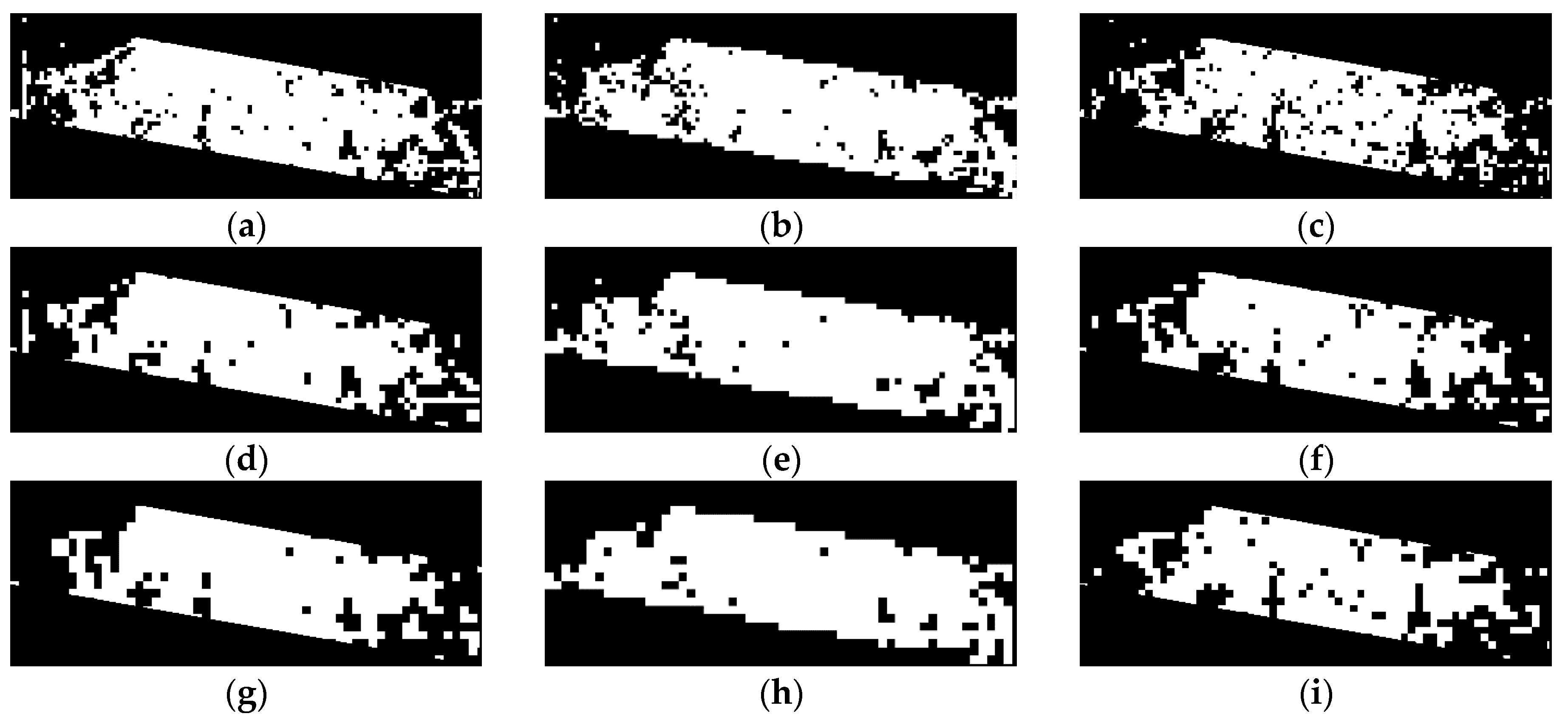
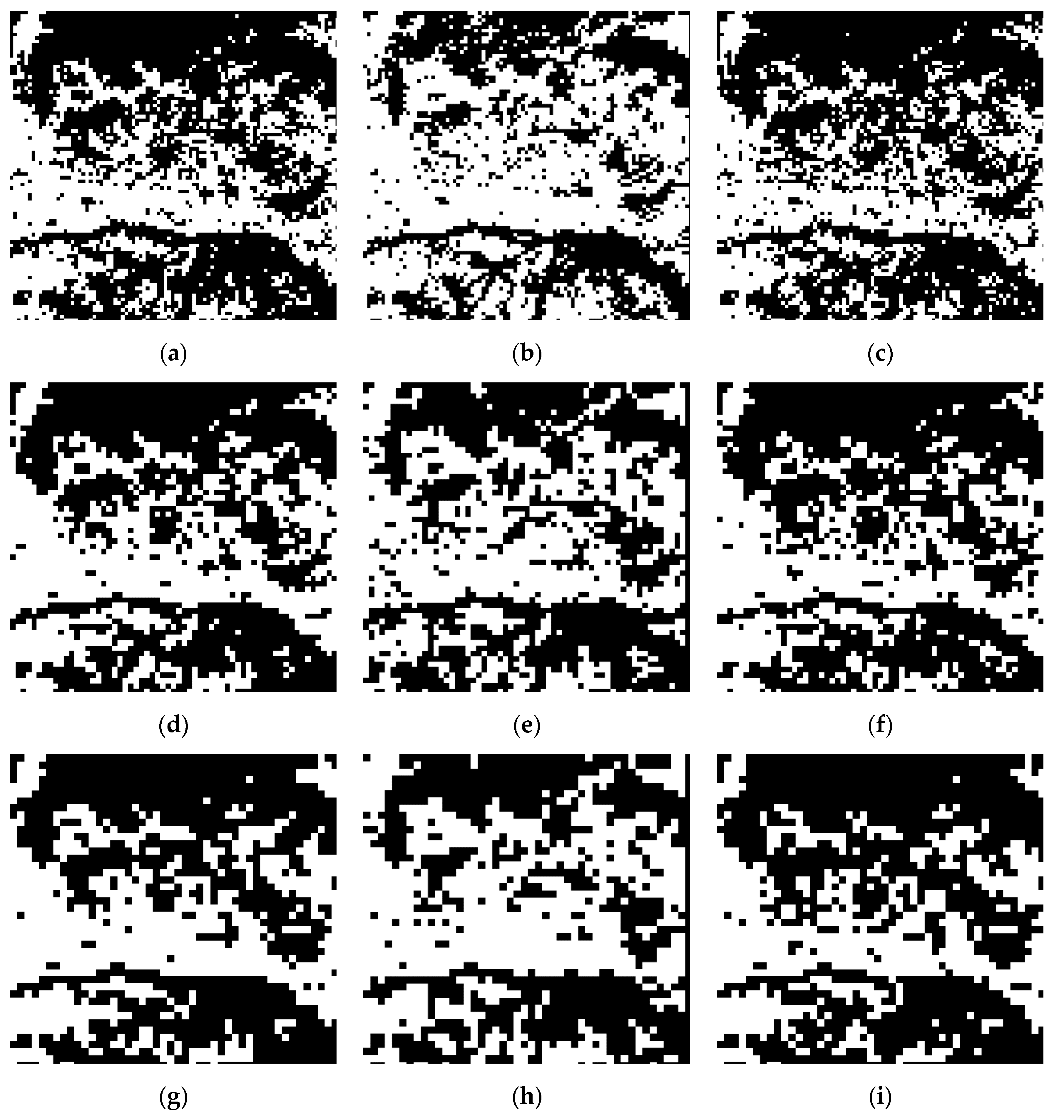
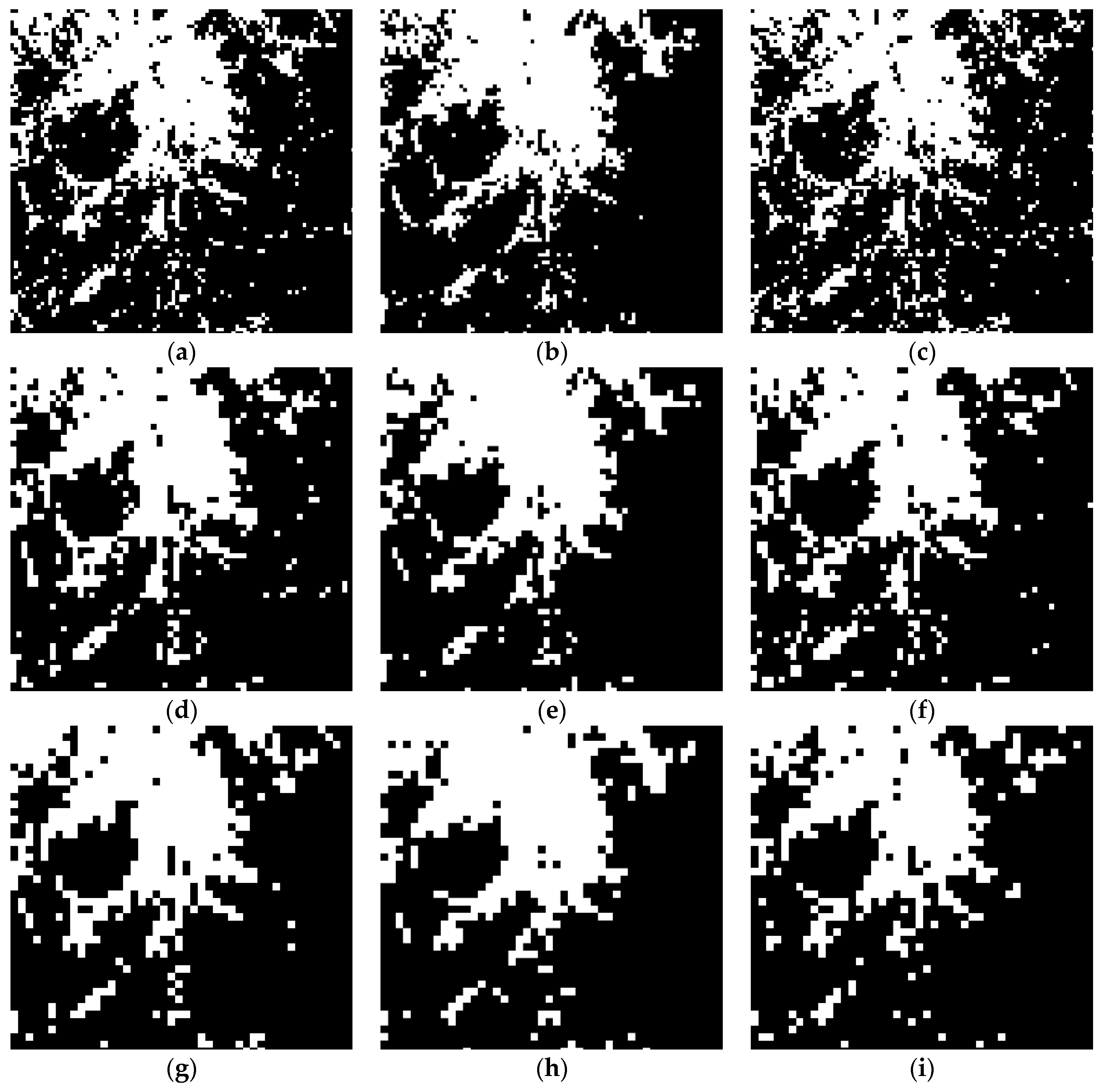
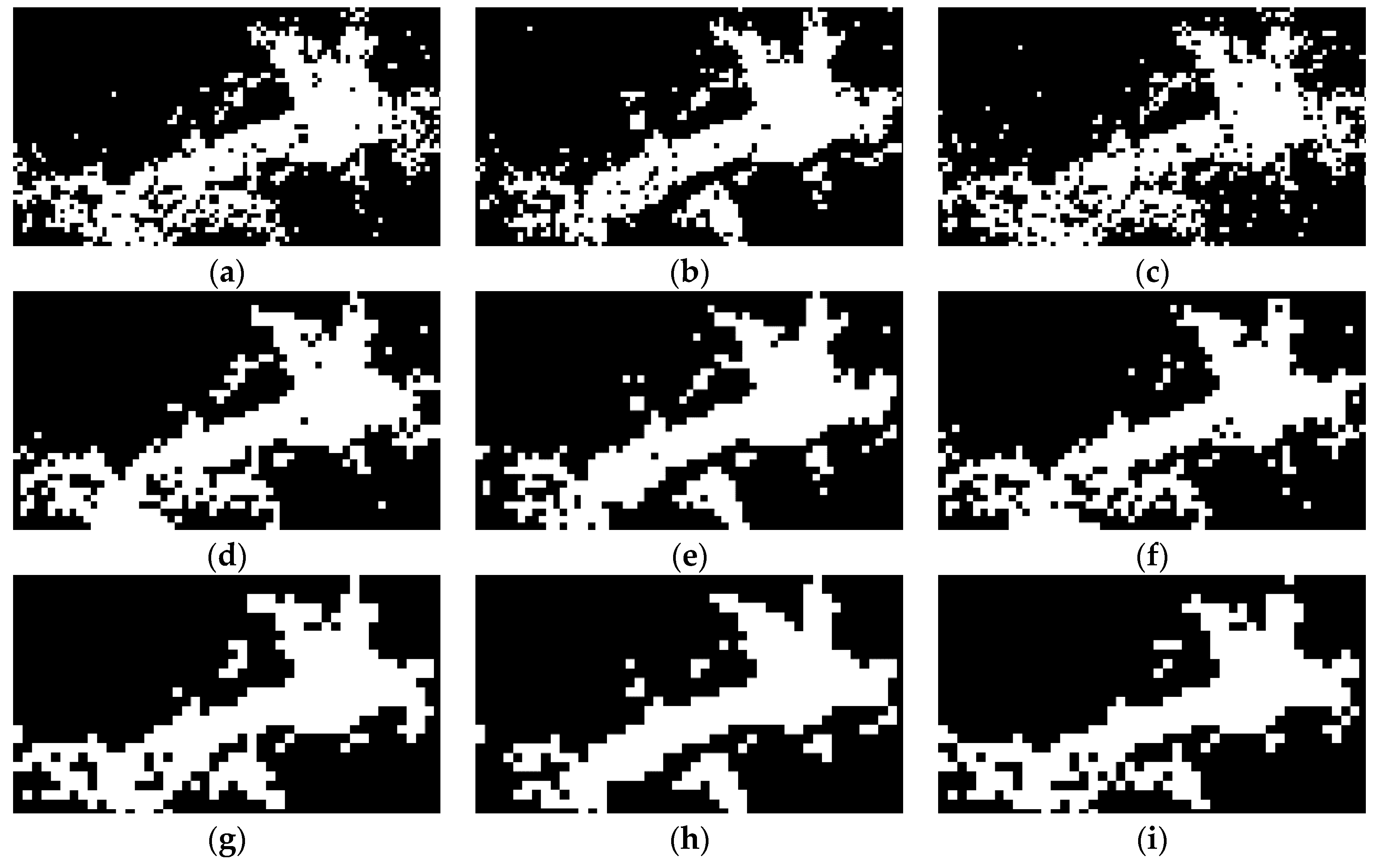
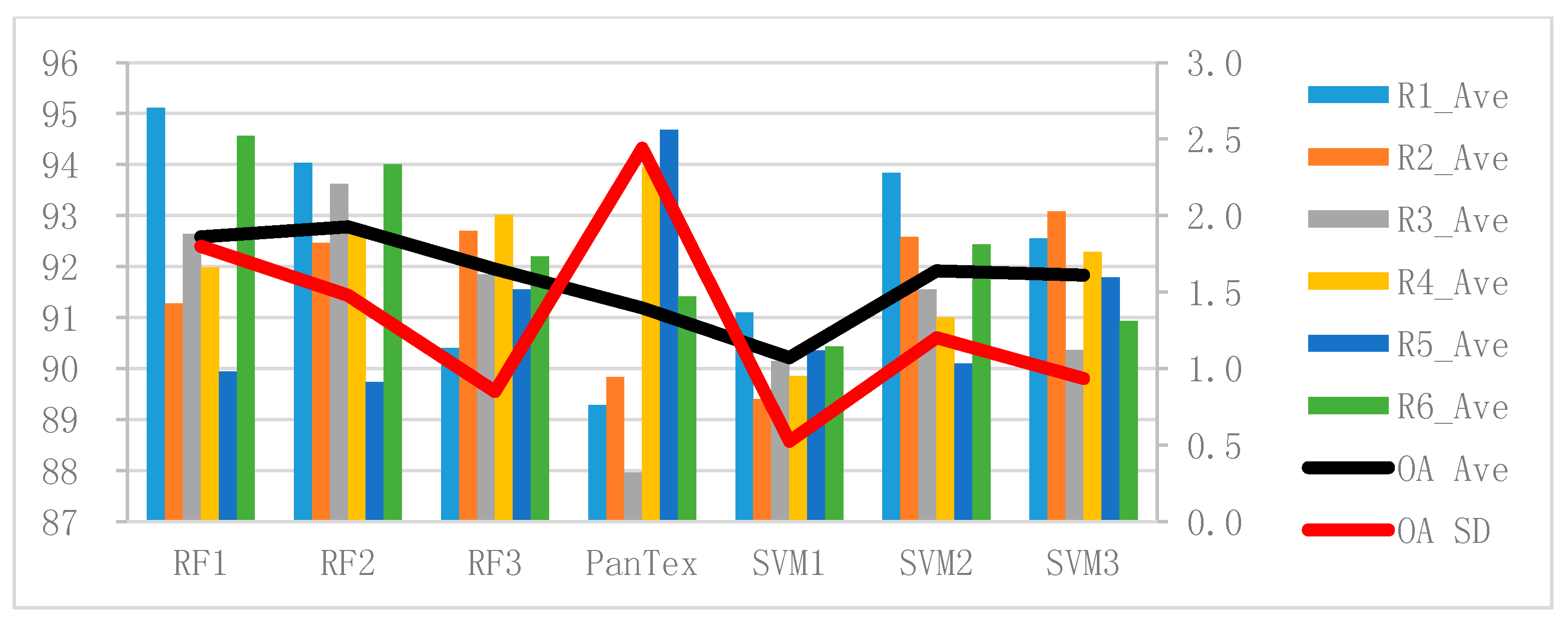
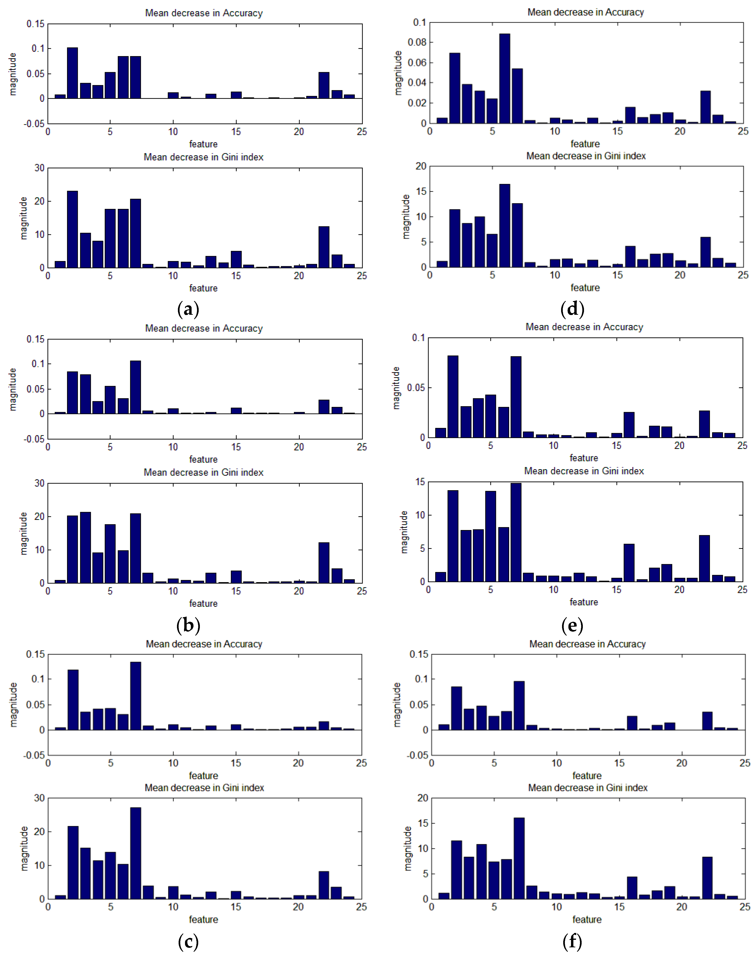
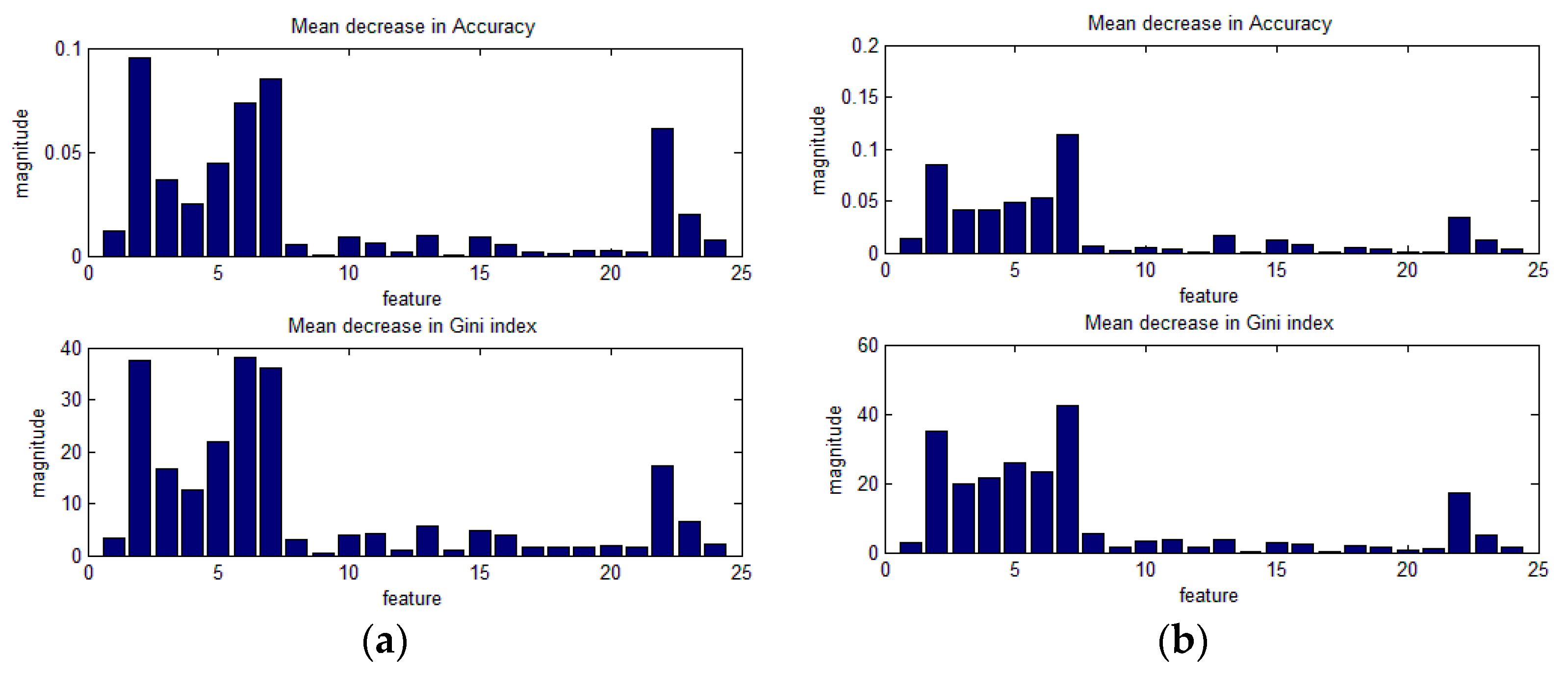
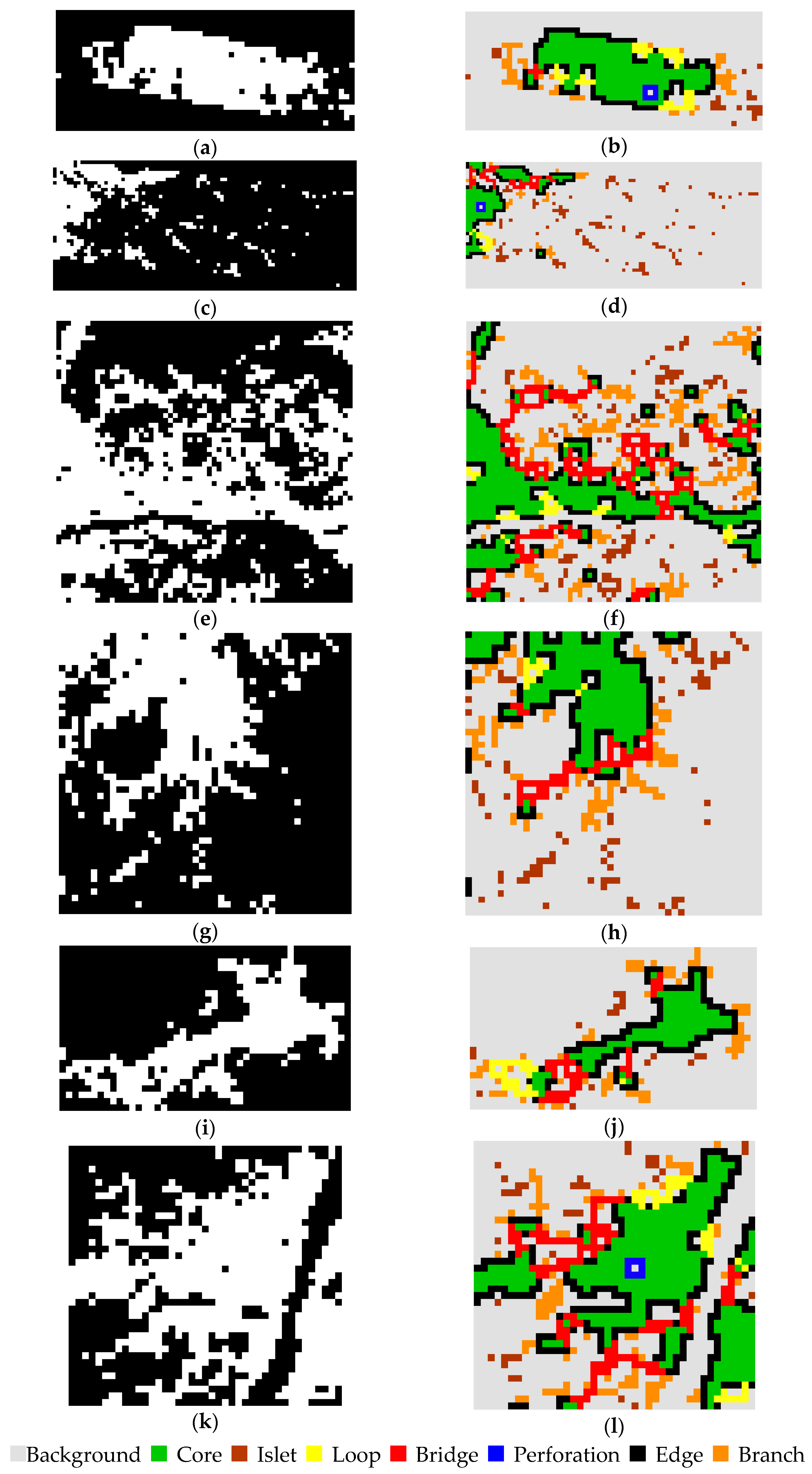
Table 1.
The parameters of the images.
| Image | Satellite | Size | Acquisition Time | Resolution (m) | City |
|---|---|---|---|---|---|
| R1 | WV-2 | 9050 × 3560 | 20 September 2011 | 2 | Harbin, Heilongjiang |
| R2 | WV-2 | 8810 × 3720 | 14 September 2011 | 2 | Harbin, Heilongjiang |
| R3 | GF-2 | 7300 × 6908 | 23 January 2015 | 4 | Guangzhou, Guangdong |
| R4 | GF-2 | 7300 × 6908 | 8 May 2015 | 4 | Urumqi, Xinjiang |
| R5 | GF-2 | 7300 × 4077 | 10 November 2014 | 4 | Lhasa, Xinjiang |
| R6 | GF-2 | 7300 × 6908 | 12 February 2015 | 4 | Wuhan, Hubei |
Table 2.
The high-level features extracted from the primitive feature maps.
| Primitive Feature Map | High-Level Features | Scale | Feature No. |
|---|---|---|---|
| MBI + NDVI | f2area: The percentage of the MBI and NDVI area | [0–100] | 1 |
| MBI | A_MBI: Percentage of the MBI area | [0–100] | 2 |
| Qua_MBI: MBI area percentage in four quadrants | [0–100] | 3–6 | |
| num_MBI: The number of MBI plots that have areas >500, 300, and 20 pixels | [0–100] | 7–9 | |
| area_MBI: The percentage of MBI plots that have areas >500, 300, and 20 pixels | [0–100] | 10–12 | |
| NDVI | A_NDVI: Percentage of NDVI area | [0–100] | 13 |
| big_NDVI: The number and area percentage of NDVI plots that have an area >500 | [0–100] | 14–15 | |
| Line segments | num_EDline: Number of line segments with length >10 pixels | >0 | 16 |
| difv: angle difference between the two top dominant directions | [0–180] | 17 | |
| DLR: Percentage of dominant direction line segments | [0–100] | 18 | |
| DLR2: Percentage of top two dominant direction line segments | [0–100] | 19 | |
| L_ls: Line length feature information: mean and variance | >0 | 20–21 | |
| MBI + NDVI + line segment | L_nb: the percentage of the MBI, the NDVI, and others in the line segment neighborhood | [0–100] | 22–24 |
Table 3.
The numbers of training and ground-truth samples of test images R1–R6.
| Image | Training | Ground-Truth | ||
|---|---|---|---|---|
| Urban | Non-Urban | Urban | Non-Urban | |
| R1 | 20 | 22 | 9,323,317 | 4,506,565 |
| R2 | 17 | 17 | 2,649,265 | 2,641,588 |
| R3 | 44 | 39 | 11,038,243 | 9,326,837 |
| R4 | 56 | 50 | 8,389,830 | 7,065,124 |
| R5 | 39 | 39 | 5,506,806 | 5,047,800 |
| R6 | 52 | 53 | 12,342,790 | 8,970,420 |
Table 4.
Accuracies (%) of image R1.
| Scale | RF1 | RF2 | RF3 | PanTex | SVM1 | SVM2 | SVM3 |
|---|---|---|---|---|---|---|---|
| 80 | 94.27 1 ± 0.12 | 92.30 2 ± 0.11 | 86.48 ± 0.36 | 90.6 | 91.4 | 92.7 | 91.3 |
| 100 | 95.69 ± 0.09 | 94.20 ± 0.30 | 88.64 ± 0.25 | 90.3 | 92.3 | 92.5 | 92.2 |
| 120 | 94.89 ± 0.15 | 94.48 ± 0.10 | 91.07 ± 0.22 | 88.9 | 92.2 | 94.5 | 92.8 |
| 140 | 95.14 ± 0.24 | 94.09 ± 0.14 | 91.84 ± 0.22 | 88.8 | 91.6 | 94.0 | 93.1 |
| 160 | 95.64 ± 0.15 | 94.89 ± 0.15 | 92.12 ± 0.17 | 88.7 | 89.1 | 94.6 | 92.8 |
| 180 | 95.04 ± 0.21 | 94.26 ± 0.11 | 92.24 ± 0.14 | 88.4 | 90.0 | 94.7 | 93.1 |
1 The red color denotes the highest OA; and 2 the bold denotes the second-highest OA at the same scale.
Table 5.
Accuracies (%) of image R2.
| Scale | RF1 | RF2 | RF3 | PanTex | SVM1 | SVM2 | SVM3 |
|---|---|---|---|---|---|---|---|
| 80 | 92.47 ± 0.27 | 93.62 1 ± 0.09 | 92.88 ± 0.17 | 91.4 | 90.2 | 92.0 | 93.2 2 |
| 100 | 92.57 ± 0.24 | 93.79 ± 0.11 | 93.52 ± 0.14 | 90.7 | 90.3 | 94.0 | 94.1 |
| 120 | 89.03 ± 0.69 | 92.46 ± 0.25 | 93.46 ± 0.13 | 90.6 | 88.7 | 93.3 | 94.0 |
| 140 | 91.39 ± 0.22 | 91.88 ± 0.22 | 92.30 ± 0.27 | 89.2 | 89.0 | 92.6 | 92.8 |
| 160 | 92.07 ± 0.12 | 91.91 ± 0.12 | 92.50 ± 0.11 | 88.6 | 89.7 | 92.0 | 93.1 |
| 180 | 90.10 ± 0.41 | 91.11 ± 0.20 | 91.53 ± 0.13 | 88.5 | 88.5 | 91.6 | 91.3 |
1 The red color denotes the highest OA; and 2 the bold denotes the second-highest OA at the same scale.
Table 6.
Accuracies (%) of image R3.
| Scale | RF1 | RF2 | RF3 | PanTex | SVM1 | SVM2 | SVM3 |
|---|---|---|---|---|---|---|---|
| 80 | 92.31 1 ± 0.11 | 92.96 2 ± 0.15 | 89.98 ± 0.12 | 87.8 | 87.6 | 89.8 | 89.5 |
| 100 | 91.47 ± 0.20 | 93.32 ± 0.08 | 90.38 ± 0.08 | 87.9 | 89.7 | 90.3 | 88.8 |
| 120 | 93.62 ± 0.14 | 94.27 ± 0.15 | 91.79 ± 0.07 | 87.8 | 92.3 | 92.7 | 91.5 |
| 140 | 93.01 ± 0.21 | 93.81 ± 0.09 | 93.01 ± 0.11 | 88.3 | 92.1 | 92.7 | 91.5 |
| 160 | 93.50 ± 0.07 | 94.23 ± 0.08 | 93.37 ± 0.12 | 88.0 | 89.6 | 91.8 | 90.9 |
| 180 | 91.92 ± 0.10 | 93.13 ± 0.12 | 92.54 ± 0.13 | 88.0 | 89.6 | 92.0 | 90.0 |
1 The bold denotes the second-highest OA; and 2 the red color denotes the highest OA at the same scale.
Table 7.
Accuracies (%) of image R4.
| Scale | RF1 | RF2 | RF3 | PanTex | SVM1 | SVM2 | SVM3 |
|---|---|---|---|---|---|---|---|
| 80 | 90.33 ± 0.16 | 91.12 ± 0.19 | 91.93 1 ± 0.12 | 94.6 2 | 87.5 | 88.7 | 90.8 |
| 100 | 91.93 ± 0.19 | 93.12 ± 0.12 | 92.88 ± 0.14 | 94.6 | 88.3 | 91.4 | 90.7 |
| 120 | 92.03 ± 0.13 | 93.38 ± 0.08 | 93.02 ± 0.20 | 94.1 | 89.4 | 90.7 | 93.0 |
| 140 | 92.29 ± 0.20 | 93.22 ± 0.21 | 93.47 ± 0.18 | 94.1 | 92.1 | 92.2 | 93.6 |
| 160 | 92.87 ± 0.24 | 92.96 ± 0.20 | 93.63 ± 0.33 | 93.4 | 91.0 | 91.7 | 92.9 |
| 180 | 92.42 ± 0.13 | 93.10 ± 0.13 | 93.14 ± 0.16 | 92.9 | 90.8 | 91.3 | 92.7 |
1 The bold denotes the second-highest OA; and 2 the red color denotes the highest OA at the same scale.
Table 8.
Accuracies (%) of image R5.
| Scale | RF1 | RF2 | RF3 | PanTex | SVM1 | SVM2 | SVM3 |
|---|---|---|---|---|---|---|---|
| 80 | 88.22 ± 0.39 | 86.20 ± 0.43 | 89.09 1 ± 0.26 | 94.0 2 | 85 | 85.4 | 87.6 |
| 100 | 88.56 ± 0.25 | 88.56 ± 0.11 | 90.18 ± 0.19 | 94.6 | 88.2 | 89.2 | 88.7 |
| 120 | 89.66 ± 0.15 | 90.12 ± 0.28 | 91.82 ± 0.15 | 94.9 | 91.9 | 89.7 | 93.3 |
| 140 | 91.84 ± 0.39 | 90.83 ± 0.37 | 92.09 ± 0.18 | 95.0 | 92.1 | 91.4 | 92.3 |
| 160 | 90.94 ± 0.43 | 91.14 ± 0.29 | 93.08 ± 0.18 | 94.8 | 91.7 | 91.6 | 93.9 |
| 180 | 90.40 ± 0.36 | 91.58 ± 0.22 | 93.02 ± 0.15 | 94.8 | 93.2 | 93.3 | 94.9 |
1 The bold denotes the second-highest OA; and 2 the red color denotes the highest OA at the same scale.
Table 9.
Accuracies (%) of image R6.
| Scale | RF1 | RF2 | RF3 | PanTex | SVM1 | SVM2 | SVM3 |
|---|---|---|---|---|---|---|---|
| 80 | 93.38 1 ± 0.16 | 92.43 ± 0.11 | 89.23 ± 0.16 | 92.8 2 | 88.5 | 90.7 | 89.0 |
| 100 | 94.26 ± 0.14 | 93.60 ± 0.11 | 91.00 ± 0.13 | 92.2 | 86.3 | 91.0 | 89.5 |
| 120 | 94.99 ± 0.14 | 94.22 ± 0.08 | 92.61 ± 0.15 | 91.2 | 90.7 | 92.1 | 91.4 |
| 140 | 94.86 ± 0.16 | 94.52 ± 0.12 | 92.82 ± 0.12 | 91.6 | 90.6 | 93.3 | 90.7 |
| 160 | 94.64 ± 0.14 | 94.47 ± 0.09 | 93.39 ± 0.13 | 90.4 | 92.8 | 93.2 | 91.7 |
| 180 | 95.23 ± 0.09 | 94.76 ± 0.10 | 94.14 ± 0.15 | 90.3 | 93.7 | 94.3 | 93.3 |
1 The red color denotes the highest OA; and 2 the bold denotes the second-highest OA at the same scale.
© 2017 by the authors. Licensee MDPI, Basel, Switzerland. This article is an open access article distributed under the terms and conditions of the Creative Commons Attribution (CC BY) license (http://creativecommons.org/licenses/by/4.0/).
Share and Cite
MDPI and ACS Style
Zhang, Q.; Huang, X.; Zhang, G. Urban Area Extraction by Regional and Line Segment Feature Fusion and Urban Morphology Analysis. Remote Sens. 2017, 9, 663. https://doi.org/10.3390/rs9070663
AMA Style
Zhang Q, Huang X, Zhang G. Urban Area Extraction by Regional and Line Segment Feature Fusion and Urban Morphology Analysis. Remote Sensing. 2017; 9(7):663. https://doi.org/10.3390/rs9070663
Chicago/Turabian StyleZhang, Qian, Xin Huang, and Guixu Zhang. 2017. "Urban Area Extraction by Regional and Line Segment Feature Fusion and Urban Morphology Analysis" Remote Sensing 9, no. 7: 663. https://doi.org/10.3390/rs9070663
Note that from the first issue of 2016, this journal uses article numbers instead of page numbers. See further details here.