An Improved Local Gradient Method for Sea Surface Wind Direction Retrieval from SAR Imagery
by
 , , , and
Lizhang Zhou
1, 
Gang Zheng
1,*,
Xiaofeng Li
2,
Jingsong Yang
1,
Lin Ren
1,
Peng Chen
1,
Huaguo Zhang
1 and
Xiulin Lou
1 1
State Key Laboratory of Satellite Ocean Environment Dynamics, Second Institute of Oceanography, State Oceanic Administration, Hangzhou 310012, China
2
GST at National Oceanic and Atmospheric Administration (NOAA)-National Environmental Satellite, Data, and Information Service (NESDIS), College Park, MD 20740, USA
*
Author to whom correspondence should be addressed.
Remote Sens. 2017, 9(7), 671; https://doi.org/10.3390/rs9070671
Submission received: 21 April 2017
/
Revised: 23 June 2017
/
Accepted: 26 June 2017
/
Published: 30 June 2017
(This article belongs to the Special Issue Ocean Remote Sensing with Synthetic Aperture Radar)
Abstract
:Sea surface wind affects the fluxes of energy, mass and momentum between the atmosphere and ocean, and therefore regional and global weather and climate. With various satellite microwave sensors, sea surface wind can be measured with large spatial coverage in almost all-weather conditions, day or night. Like any other remote sensing measurements, sea surface wind measurement is also indirect. Therefore, it is important to develop appropriate wind speed and direction retrieval models for different types of microwave instruments. In this paper, a new sea surface wind direction retrieval method from synthetic aperture radar (SAR) imagery is developed. In the method, local gradients are computed in frequency domain by combining the operation of smoothing and computing local gradients in one step to simplify the process and avoid the difference approximation. This improved local gradients (ILG) method is compared with the traditional two-dimensional fast Fourier transform (2D FFT) method and local gradients (LG) method, using interpolating wind directions from the European Centre for Medium-Range Weather Forecast (ECMWF) reanalysis data and the Cross-Calibrated Multi-Platform (CCMP) wind vector product. The sensitivities to the salt-and-pepper noise, the additive noise and the multiplicative noise are analyzed. The ILG method shows a better performance of retrieval wind directions than the other two methods.
1. Introduction
Surface wind field over the oceans is needed for weather forecasts, wind resources assessment, numerical modeling of waves, oil spill monitoring, and so on [1,2,3,4,5,6,7,8,9,10]. Traditional measurements of sea surface wind from ships, buoys and land stations are far from meeting the growing demand for human beings, as these approaches can only provide data with limited spatial and temporal coverage. Spaceborne microwave radiometers and scatterometers have provided global-scale observations for sea surface wind, but the wind data in coastal regions are missing due to contamination from signal reflection of land [11,12,13]. Also, the spatial resolution of radiometers or scatterometers is relatively low (about 25 km). This is suitable for open ocean studies. However, wind fields on a much finer scale can be provided by spaceborne synthetic aperture radar (SAR) due to its relatively high spatial resolution. As a result, SARs can be useful tools when high-resolution ocean surface wind fields are needed, especially in coastal regions, and the retrieval of wind field from SAR images is widely researched [14,15,16,17,18,19,20,21].
Many satellites have been launched with SAR onboard, e.g., Seasat, ERS-1/2, Envisat, Radarsat-1/2, and so on [14,15,16,17,18]. These sensors have acquired abundant SAR images containing many interesting features including coastal upwelling, typhoon/hurricane, atmospheric waves, atmospheric vortex street, and so on [19,20,21,22,23,24,25,26,27,28,29,30,31]. Some of SAR imaged features, e.g., Langmuir cells, boundary layer rolls, surfactant streaks, foam and water blown from breaking waves, or wind shadowing, align with wind direction.
Wind direction (with an ambiguity of 180°) can be retrieved from these features by different methods including Fourier transforms, wavelet analysis, local gradients and so on. The 180° ambiguity can be removed by referencing to weather model output, Doppler shift or land shadows [3,16,32]. The accuracy of various methods ranges from 15–40° [33]. After wind direction is obtained, wind speed can be retrieved by physical or empirical models. Accordingly, estimating wind vectors directly from SAR images becomes feasible [34]. Both cross-polarization and co-polarization SAR images can be used for the retrieval of wind vectors [35,36,37]. There are two conventional methods of retrieving wind directions (with an ambiguity of 180° which is removed later) from SAR images, namely, two-dimensional fast Fourier transform (2D FFT) method and local gradients (LG) method [34,38,39]. In the FFT method, the Fourier spectrum of SAR images is computed and the main spectral energy is located perpendicular to the orientation of the wind streaks. The reported standard deviations of FFT method are between 10–37° and the method works fine on large image areas, e.g., 20 km by 20 km [34]. In the LG method, local gradients are computed with standard image processing algorithms, and the orthogonal of the most frequent gradient direction is chosen to be the likely wind direction. The reported directional error of LG method was about 20° for ERS-1/2 images and the most frequent spatial sampling used was 20 km by 20 km and 10 km by 10 km [34].
The tests in [34] indicated that the LG method could provide a higher resolution of retrieved wind field than the FFT method. However, the current LG method has a problem; that is, the local gradients in the conventional LG method are computed with difference approximation like Sobel operators, and this process is easily affected by noise, e.g., speckle noise. Thus, SAR images are usually first smoothed before computing local gradients. In this study, we develop an improved local gradients (ILG) method for sea surface wind retrieval by combining smoothing and computation of the local gradients together in the frequency domain. In the method, the computation of local gradients is analytical as the Gaussian function can be expressed analytically in both spatial domain and frequency domain and it can avoid the errors of difference approximation which can be easily affected by noise. The new method is tested on the images acquired by the advanced synthetic aperture radar (ASAR) onboard Envisat, and its retrieved results show better agreement with both following kinds of interpolating wind directions than the other two methods. The interpolating wind directions from the European Centre for Medium-Range Weather Forecast (ECMWF) reanalysis data are obtained by interpolating the ECMWF reanalysis data to the SAR imaging times. The same procedure is applied to the Cross-Calibrated Multi-Platform (CCMP) data to obtain the interpolating wind directions from the CCMP data.
The remaining sections are organized as follows. In Section 2, the ILG method is described in detail. In Section 3, the data sets used are introduced. In Section 4, we compare the three wind direction retrieval methods using the wind directions from the ECMWF reanalysis data and the CCMP wind products. The ILG method is also tested by using small images (thus high resolution) in this section. The performance of each retrieval method is analyzed while the images are corrupted by different types of noise in Section 5. Conclusions are given in Section 6.
2. Improved Local Gradients Method
The direction of the gradient should be the same as the direction of the strongest change in an image, and an ideal image of streaks should have nearly no change along the direction of streaks, and show the strongest variation in the orthogonal direction of streaks. Thus, the wind direction, which is assumed to be parallel to the wind streaks [40], is also perpendicular to the direction of the gradient. Usually, the components of the gradient are computed with the optimized Sobel operators pixel by pixel after smoothing, and the most frequent gradient direction is chosen to be the local wind direction.
As mentioned in the introduction, the computing method described above, however, can lead to some problems. So, we try to combine the operation of smoothing and computation of local gradients on the basis of a conventional LG method which is given by Koch in 2004. The smoothing of an image can be realized by convolution, and the Gaussian function is commonly used for smoothing, as shown in
where is the image after smoothing, and is the original image. is the Gaussian function for smoothing, with the form
where σ determines the width of smoothing window in the ILG method. The choice of the value of the parameter is empirical, and in this paper the parameter is set to 15 for all SAR images. The benefit of the choice of the Gaussian is that it can be expressed analytically in both spatial and frequency domains. The gradients of the image can be expressed as
where and are the unit vectors in the x and y directions, respectively. Using Equation (1)–(3) and exchanging the order of integral and partial derivative, can be expressed as
where * denotes convolution, and . We perform Fourier transform on both sides of Equation (4), and get
where denotes the 2D Fourier transform.
The first term on the right hand side of Equation (5) can be obtained from the Fourier transform of the image directly. The second term, represented by for convenience of expression, can be expressed as
where i indicates the imaginary part. So, can be expressed as
where denotes the 2D inverse Fast Fourier transform (2D IFFT). Similarly, can be expressed as
where can be expressed by Equation (9).
and are denoted as and , respectively, for convenience, so the gradients can be stored as complex numbers in the form of
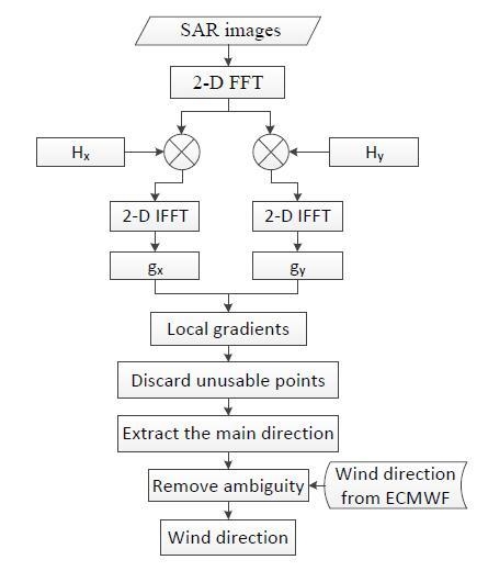
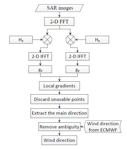
Now, the gradients are in the same form as those in Koch’s LG method [34]. Figure 1 shows the flowchart of the ILG method for wind direction retrieval. The remaining steps are consistent with those in Koch’s method, including discarding unusable points and extracting the main gradient direction. The 180° wind direction ambiguity is removed by referencing coincident wind direction from the ECMWF model result [41].
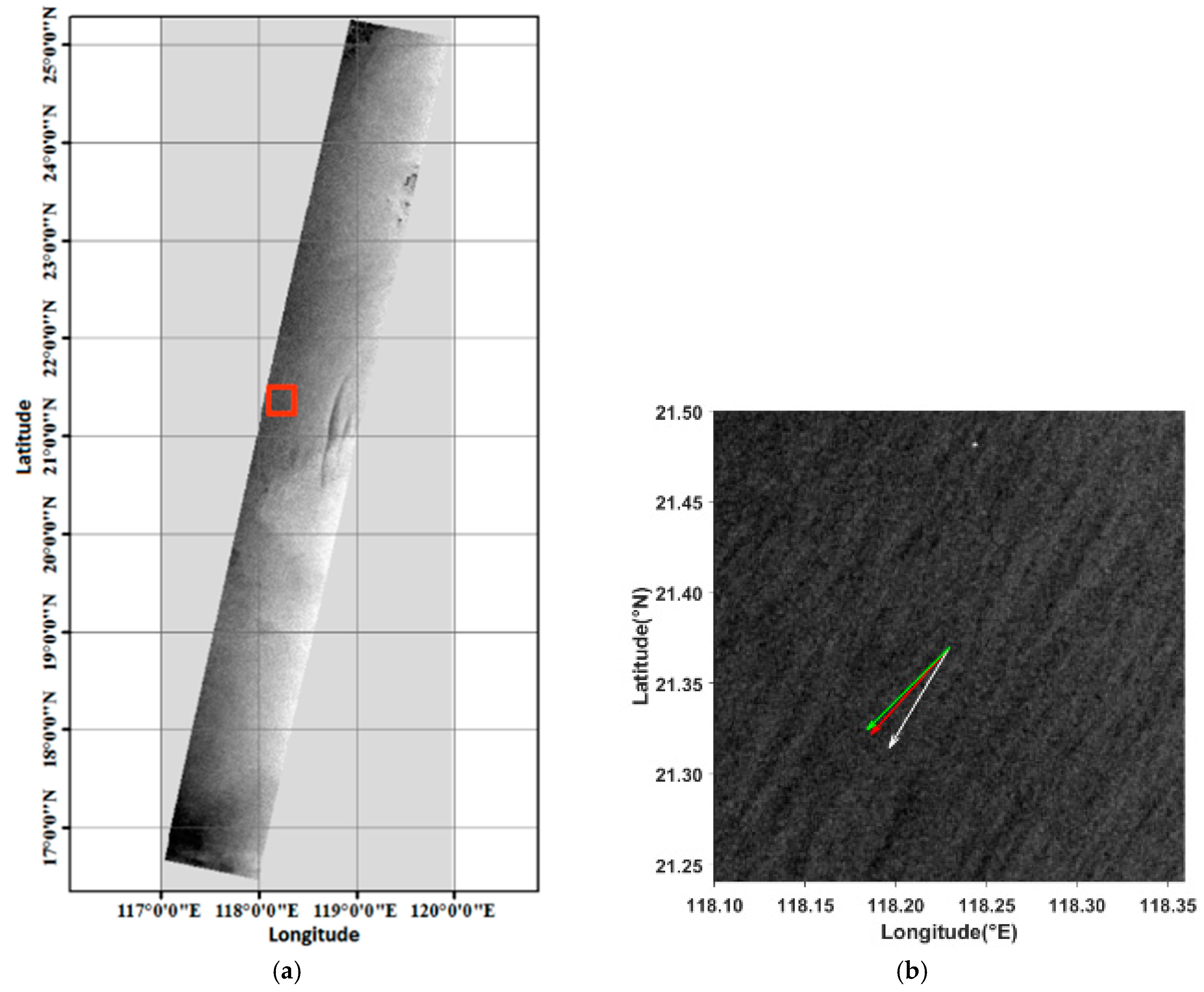
The image acquired by the advanced synthetic aperture radar (ASAR) onboard Envisat at 02:06 on 14 October 2007 is shown in Figure 2a. Figure 2b shows the wind direction computed on a 30 km by 30 km subimage which is indicated by red box in Figure 2a. Wind streaks are visible all over the subimage. The white arrow (211°) in Figure 2b indicates the wind direction computed from 75 m pixels by using the ILG method. The wind direction from the ECMWF was 222°, indicated by the red arrow in Figure 2b. The wind direction from the CCMP was 225° (the green arrow in Figure 2b). Note that the wind directions here are placed in the same coordinate. In this coordinate, the direction of the northward wind vector is 0° (or 360°), the direction of the eastward wind vector is 90°, the direction of the southward wind vector is 180°, and the direction of the westward wind vector is 270°.
3. Data Sets
3.1. SAR Data
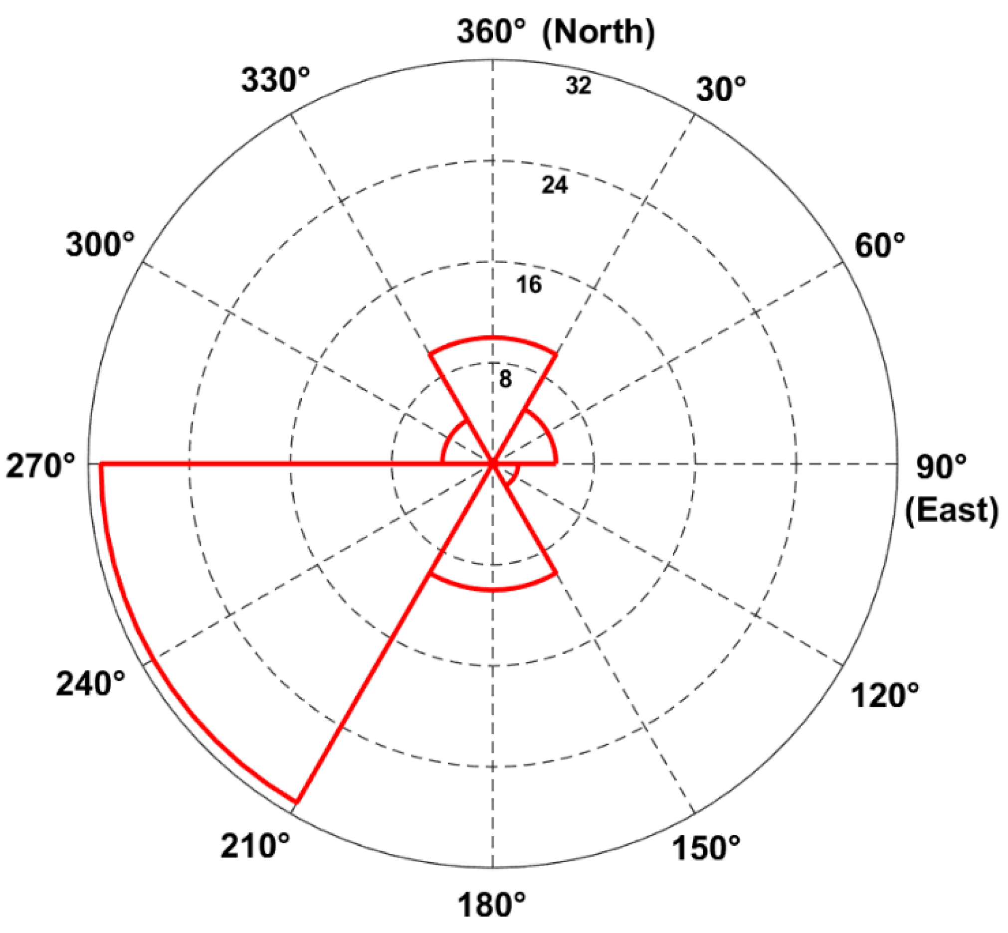
The wind streaks do not appear in all regions of the full-frame SAR image, so we find the wind streak patterns in a SAR image and apply the retrieval methods to the sub-images at these locations. After that, we can validate the retrieval results against the interpolating wind directions at these locations. To compare the retrieved results of different methods with the CCMP products on 0.25° grid, we test all methods over the 30 km by 30 km sub-images, uniformly. Finally, we acquired 62 Envisat ASAR sub-images between 2004 and 2011. Most of the images are located between 15°N to 35°N and 113°E to 129°E. ASAR operates in the C band in a wide variety of acquisition modes. The incidence angles of ASAR range from 15° to 45°. The ASAR images used here are in VV polarization with a spatial resolution of 75 m by 75 m in range and azimuth. Geometric calibrations are carried out by the Next ESA SAR Toolbox provided by the European Space Agency (ESA). The distribution of wind directions of all ASAR images used in the study is shown in Figure 5. The radius of each fan indicates the amount of wind directions in each interval.
3.2. ECMWF Data
The ERA-Interim is the latest global atmospheric reanalysis produced by ECMWF. The ERA-Interim reanalysis is produced with data assimilation, advancing forward using 12-hourly analysis cycles in time. In each cycle, available observations and prior information from a forecast model are combined to obtain the evolving state of the global atmosphere and its underlying surface. Thus, the data assimilation produces 6-hourly products at different spatial resolutions, which include various kinds of global surface parameters including and wind components at 10 m height [42]. It covers a long period starting in 1979 and continues updating in near real time. The detailed method for extracting the wind direction of a specific SAR image from the ECMWF data (0.25°) is as follows. First, the nearest location is found by the latitude and longitude of the center of the SAR image. Then, the u and v components at imaging time are obtained by interpolating the reanalysis data of the nearest two times. At last, the wind direction is computed by using the u and v components from interpolation.
3.3. CCMP Data
The wind directions from the CCMP wind product are used for validation. The CCMP data set combines cross-calibrated satellite microwave winds and instrument observations to produce high-resolution (0.25°) gridded analysis using a 4-dimensional variational analysis method with the ECWMF ERA-Interim Reanalysis model wind field as a background wind. Each daily data file contains three arrays of size 1440 (longitude) by 628 (from 78.375°S to 78.375°N) by 4 (times of 0, 6, 12 and 18 UTC) [9]. Two of the arrays are u and v wind components in meters per second at 10 m height. Another array in the file is the number of observations (satellites or buoys) used to derive the wind components for each grid and a number of observations value of zero means that the wind vector for this grid was obtained from the background field only as no satellite or moored buoy wind data were available. We prefer the data from satellite or instruments, so only the locations where the number of observations is more than zero are taken into consideration. The steps for extracting the wind direction of a specific SAR image from the CCMP data are similar to that from the ECMWF data.
4. Results and Discussion
To compare the results of different wind direction retrieval methods, the wind directions interpolated from ECMWF and CCMP data are used, respectively. For each 30 km by 30 km image, the interpolating wind direction was obtained by the nearest grid from the center of the image. Furthermore, the performance of the ILG and the other two methods for small regions (e.g., 7.5 km, 6 km and 3 km) is discussed visually. We implemented the FFT and LG method based on algorithms described in the papers [34,38]. Therefore, we specify these methods as FFT-like method and LG-like method to suggest that they are our implementation of the original wind direction retrieval techniques, respectively.
4.1. Comparison with ECMWF
In this part, the wind directions interpolated from ECMWF data are used to compare the retrieved results of different methods. Figure 6 shows the comparison between the retrieved result of each method and ECMWF wind directions for all 62 images, and each dot represents the retrieved wind direction and the wind direction interpolated from ECMWF data.
From Figure 6, we can see that the wind directions retrieved by each method are obviously correlated with those from the ECMWF reanalysis data for these images. Table 1 shows the root-mean-square (RMS) error, correlation coefficient (R) and p-value (p-value demonstrates whether the two sets of data are correlated and the significance of correlation is larger when its value is smaller) of wind direction comparisons obtained by different retrieval methods and the ECMWF reanalysis data. In addition, if the absolute value of the angle difference between the retrieved direction and the ECMWF reanalysis data is bigger than 90°, the retrieved direction should add or subtract 360° before computing these statistics, e.g., the retrieved direction is 2° and the direction from ECMWF is 358°, so the retrieved direction should be converted to 362°. The process is similar for the computation with the CCMP data. We can see that the wind directions retrieved by the ILG method are closer to those of ECMWF reanalysis with the least RMS error of 21.57° and the largest correlation coefficient of 0.9765. In addition, the p-value of ILG method is the smallest among the three methods. These statistics indicate that the retrieved results of the ILG method are the closest to the ECMWF reanalysis data among the three methods. By the way, the directional error of LG method in Koch’s paper is 17.6° for ERS-1/2 images, but there are no details about how to obtain the value. In fact, the validation results could be affected by several factors (e.g., the ground truth data, difference of different SAR sensors). In our study, we tested the different methods using ASAR images and the ECMWF (or CCMP) data, in order to compare their performances fairly. As a result, the statistics are different.
4.2. Comparison with CCMP
We prefer the CCMP data with observations (satellites or buoys), and we matched up SAR images with the CCMP data which have observations. Finally, 22 images are matched. Figure 7 shows the comparison between the results of each method and CCMP wind directions for all matched images.
From Figure 7, we can see that the wind directions retrieved by each method show an obvious correlation with those from CCMP data for the matched images. Table 2 shows the results of statistics between wind directions obtained by each retrieval method and CCMP for these matched images. We can see that wind directions retrieved by the ILG method is the closest to the CCMP data with the least RMS error of 21.61° and the largest correlation coefficient of 0.9771. The p-value of ILG method is also the smallest. Consequently, the wind directions retrieved by the ILG method are the closest to CCMP data among the three methods.
4.3. Discussion
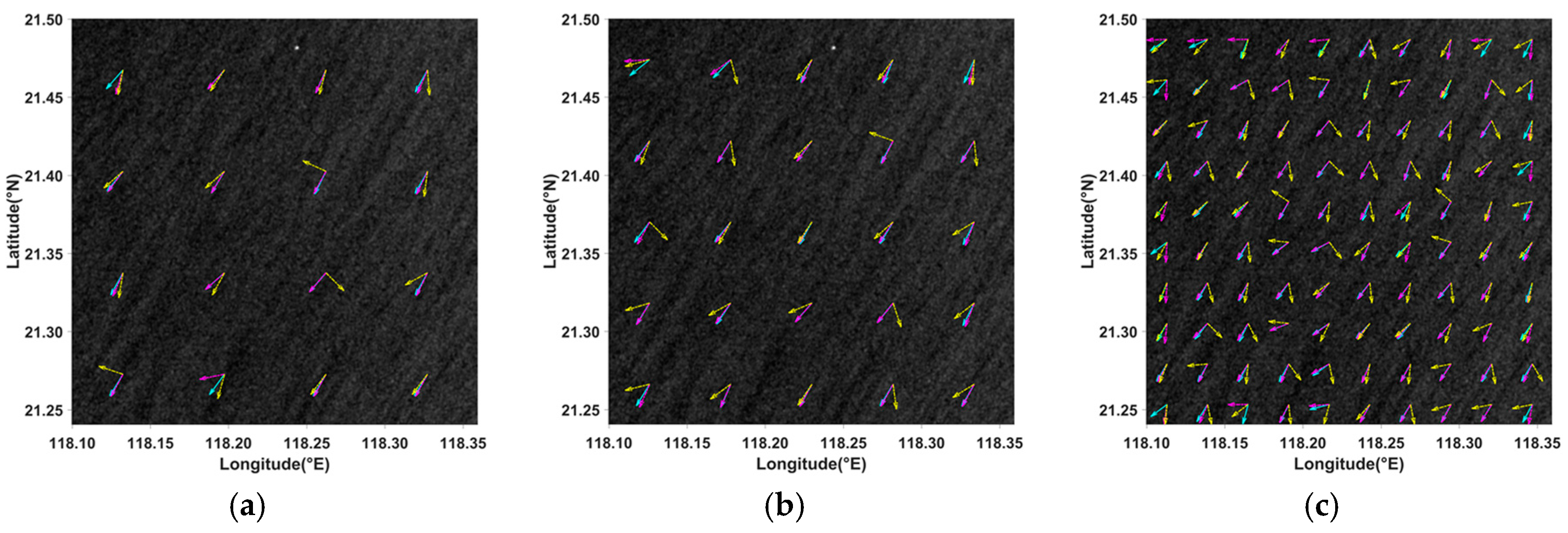
The wind directions discussed above are retrieved from 30 km by 30 km images with a spatial resolution of 75 m in both range and azimuth. To test the performance of the ILG method in small regions, wind directions of the example image in Figure 2b are computed on 7.5 km, 6 km and 3 km grids, respectively. The other two retrieval methods are also carried out on the same grids. Figure 8 shows the results of the three retrieval methods of the image on different grids. Yellow, magenta and cyan arrows indicate wind directions retrieved by the FFT-like, LG-like and ILG methods, respectively. The general wind direction of the image is from upper right to lower left. On the three kinds of grids in Figure 8, the retrieved results of the FFT-like method does not work well, and the retrieved results of the LG-like and ILG methods agree well with the streaks in the most areas. However, the retrieved results of the ILG method show better agreement with the streaks than that of the ILG method on the grids where the retrieved results of the two methods differ, visually. Another ASAR image acquired at 00:45, 25 March 2005 in VV polarization with a spatial resolution of 75 m was also tested. The image was along the coastal area of Iwate Prefecture, Japan. Figure 9 shows the image and the retrieved results of the three methods on 7.5 km, 6 km and 3 km grids, respectively. Yellow, magenta and cyan arrows indicate the wind directions retrieved by the FFT-like method, LG-like and ILG methods, respectively. From the SAR image, it can be seen that the general wind blows from upper left to lower right. From Figure 9a–c, we can see that the retrieved wind directions of the LG-like and ILG methods show better agreement with the streaks in most regions than the results of the FFT-like method. The retrieved wind directions of the ILG method still agree better with the general wind direction than the other two methods at the bottom of the image with the influence of the land.
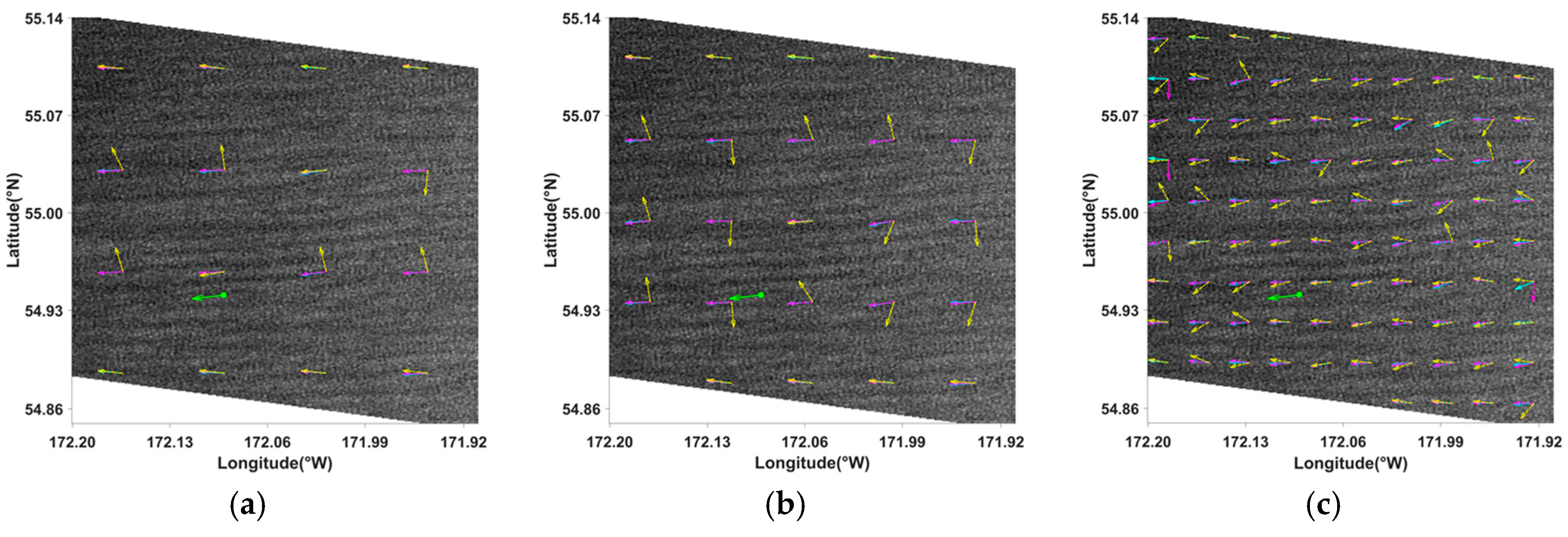
We have tried to match all the ASAR sub-images we have with buoys, but none are matched. However, a Radarsat-2 image is matched with the buoy (46073) of National Data Buoy Center (NDBC). The Radarsat-2 image was acquired at 17:58, 11 February 2011 in VV polarization, and it was reduced to 80 m by 80 m. A region (32 km by 32 km) where the wind streaks are visible was cut out to perform the test. Figure 10 shows the results of the three retrieval methods of the sub-image on different grids (8 km, 6.4 km and 3.2 km), and the buoy is marked as a green dot in the SAR image. Again, the yellow, magenta and cyan arrows indicate wind directions retrieved by the FFT-like, LG-like and ILG methods, respectively. The wind direction (263°) measured by the buoy is indicated by the green arrow. From Figure 10, it can be seen that the retrieved wind directions of the LG-like and ILG methods agree better with the wind direction measured by the buoy than the FFT-like method. From Figure 10c, it can be seen that the retrieved results of the LG-like and ILG methods agree with each other in most regions, but the retrieved results of the ILG method show better agreement with the streaks than that of the LG method, especially at the edges of the SAR image.
5. Sensitivities to Different Noise
In the conventional LG method, the local gradients are computed using difference operators (e.g., Sobel operators), which is easily affected by noise. However, the ILG method does not need any difference approximation. Therefore, the sensitivities of the three retrieval methods to different types of noise are analyzed, including the salt-and-pepper noise, the additive noise and the multiplicative noise. It is assumed that there is no noise in the original SAR images before they are corrupted by the noise in the tests. Figure 11 shows the image corrupted by different noise, taking the image in Figure 2b as an example. For a specific kind of noise with a specific intensity, the RMS of a specific method was calculated from the differences between the retrieved results of the 62 corrupted images by the method and those interpolated from the ECMWF data. After we calculate the RMS differences of the method for different intensity, we get the RMS curve of the method with respect to intensity for the kind of noise. The RMS curves are used to compare the sensitivity of each method. The same procedure was done for the 22 images matched with CCMP data.
5.1. Salt-and-Pepper Noise
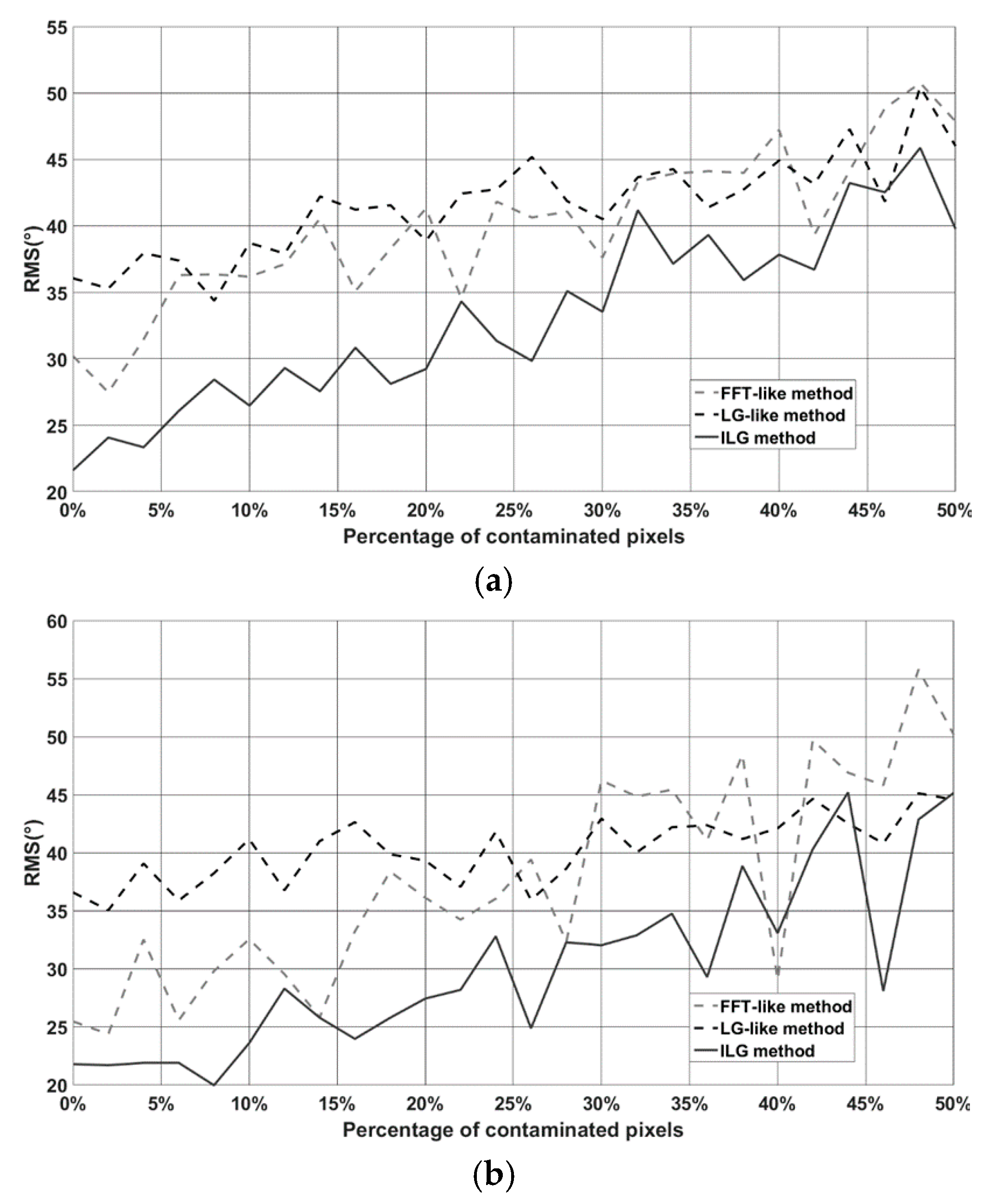
Figure 12 shows the RMS differences between each of the three retrieval methods and interpolating wind directions of ECMWF or CCMP data when the salt-and-pepper noise exists in each image with different intensities. The intensity of the salt-and-pepper noise is decided by the percentage of contaminated pixels in the image. It is obvious that the quality of wind direction retrieval roughly decreases with the increase of noise level. The curve of the ILG method is below the curves of the other two methods in Figure 12a,b. It indicates that the ILG method can achieve better retrieved results than the other two methods comparing with ECMWF (or CCMP) data when the salt-and-pepper noise exists.
5.2. Additive Noise
The additive noise is added to the image I using the equation
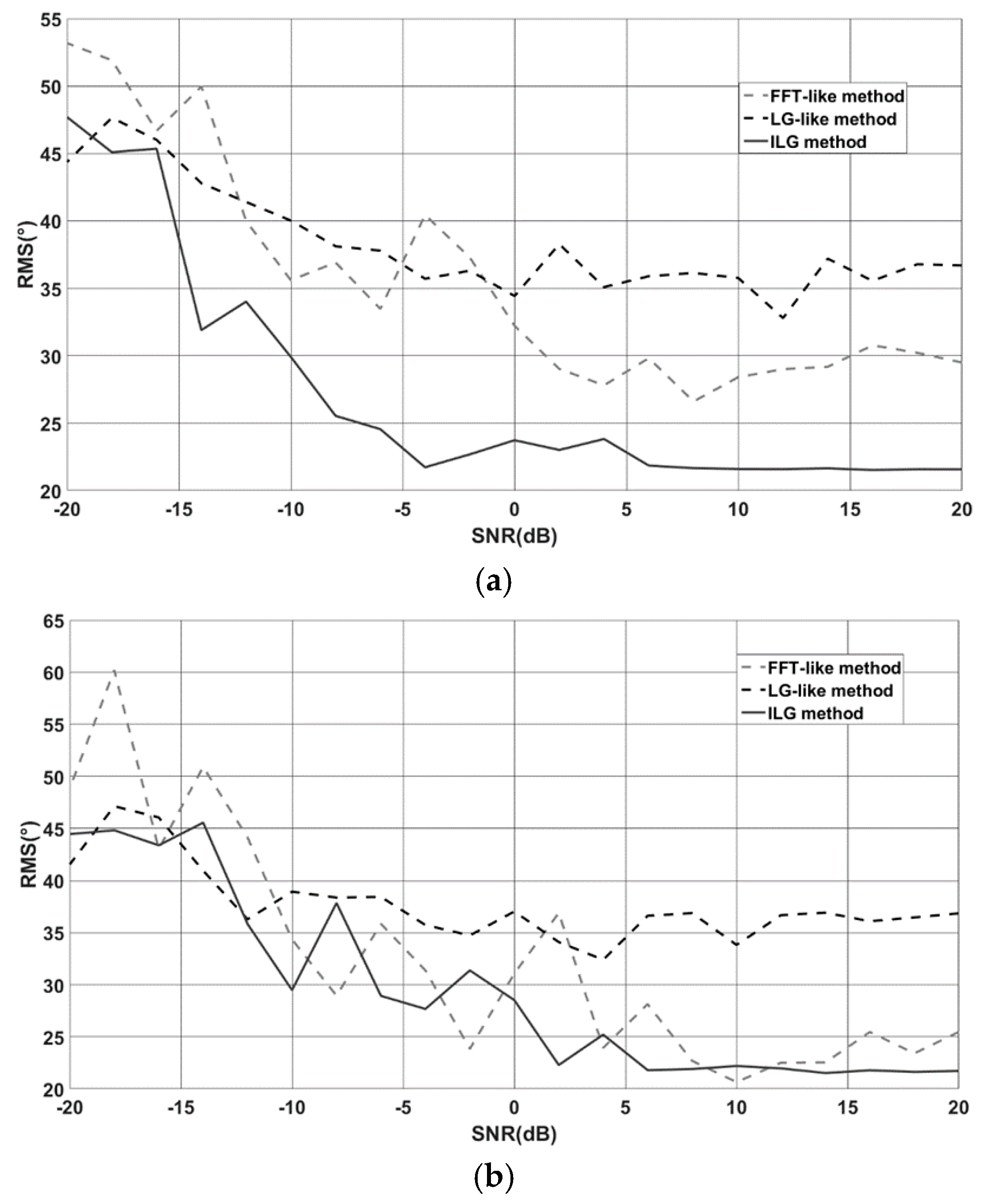
where n is the Gaussian white noise with zero mean and a specific variance. As mentioned above, it is assumed that there is no noise in the original SAR images before they are corrupted by the noise in the tests. Therefore, the signal-to-noise ratio (SNR) of an image corrupted by noise can be considered as the ratio of the variance of the original image and the variance of n. The intensity of the noise is lower when the SNR is larger. Figure 13 shows the RMS differences between the results of the three retrieval methods and interpolating wind directions when the images are corrupted by the additive noise with different SNR. We can find that all curves decline with increasing SNR, roughly. Furthermore, the ILG method can achieve better retrieved results than the other two methods comparing with ECMWF (or CCMP) data when the additive noise is present.
5.3. Multiplicative Noise
The multiplicative noise is added to the image I using the equation
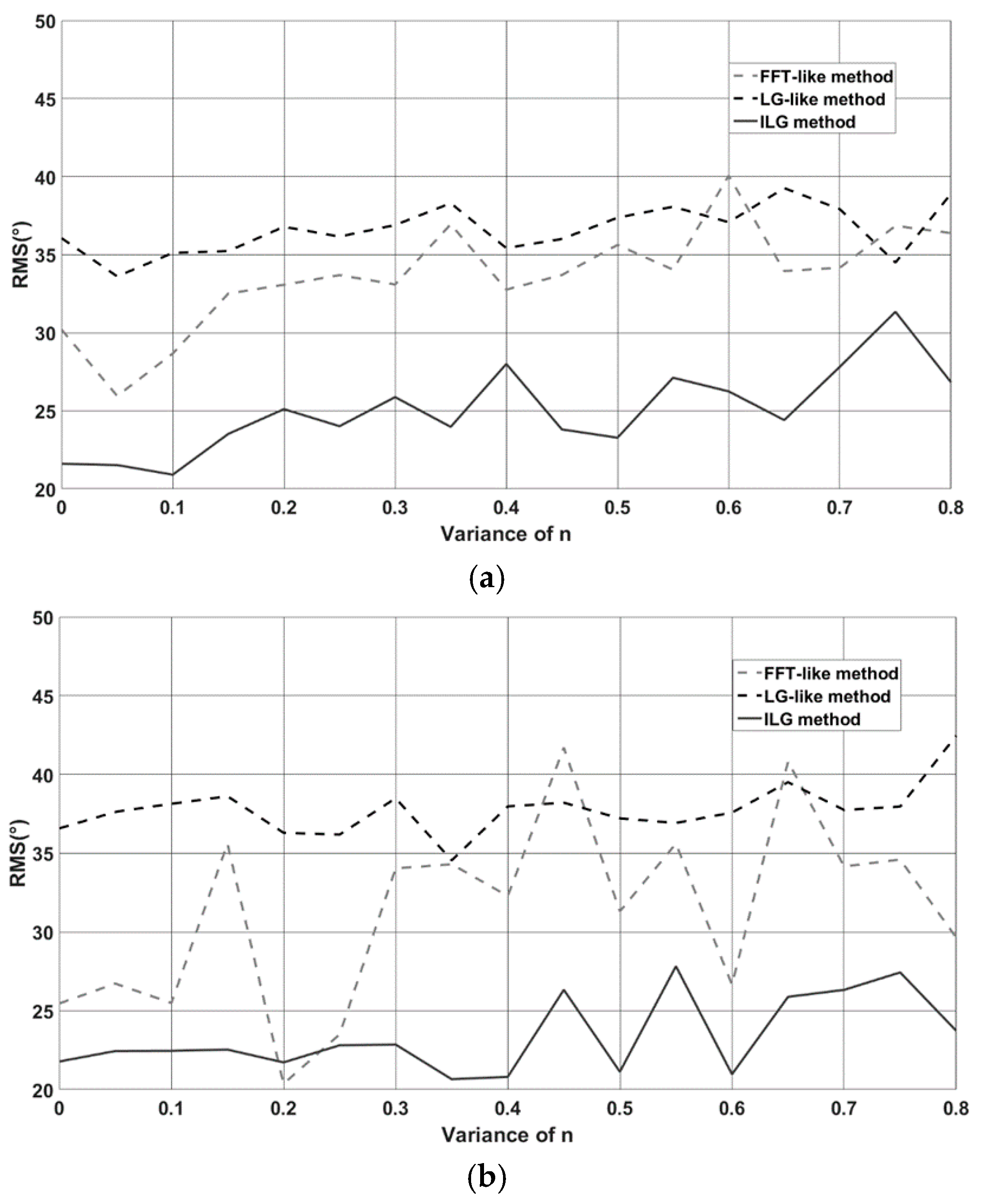
where n is uniformly distributed random noise with zero mean and a given variance. The multiplicative noise intensity is decided by the given variance. The noise intensity increases with the increase of the variance. Figure 14 shows the RMS differences between the results of the three retrieval methods and interpolating wind directions while the multiplicative noise changes with different variance. The retrieved results of the three methods become worse roughly while the noise becomes greater. However, the ILG method always gives better retrieved results than the other two methods when the multiplicative noise is present comparing with ECMWF (or CCMP) data.
The speckle noise is a kind of multiplicative noise as well, but the equation used to add the speckle noise to the image I is a little different from Equation (12), which can be described as:
where n is the noise with an exponential distribution whose expectation and variance are 1, as the SAR intensity images are corrupted. The RMS difference of each method between retrieved results of the images corrupted by this noise and wind directions obtained from the ECMWF (or CCMP) data is shown in Table 3. From Table 3, it can be seen that the retrieved results of the corrupted images of each method become worse than the results in Table 1 and Table 2, as the speckle noise affects the retrieved results. However, the retrieved results of the corrupted images by the ILG method are better than the other two methods comparing with ECMWF (or CCMP) data when the speckle noise exists.
Form the analysis above, it can be found that the sensitivity of the ILG method to each kind of noise is lower than the other two methods.
6. Conclusions
In this study, the conventional LG method was improved by using the new approach to compute the local gradients. With the new approach, we can avoid the difference approximation which can be easily affected by noise. Comparing with ECMWF and CCMP data, we found that the RMS difference of the ILG method is smaller (about 15°) than the FFT-like and LG-like methods. The correlation coefficient of ILG method is the largest (about 0.98) among the three methods, suggesting that its retrieved results fit the ECMWF and CCMP data better than the other two methods. The ILG method could retrieve wind directions from small images (thus high resolution) with the tests on different grids, and the retrieved results of the ILG method on small grids (e.g., 3 km) agree better with the wind streaks than the other two methods. When the SAR images containing both sea and land portions are processed, the ILG method still can work well. Furthermore, the sensitivity of the ILG method to different noises is lower than the other two methods, as the new method can avoid the use of difference approximation operators. All of these indicate that the ILG method is feasible.
Acknowledgments
This work is supported by the National Natural Science Foundation of China (Nos. 41676167, 41306192, 41476088, 41576174 and 41621064), the National Key R&D Program of China (Nos. 2016YFC1401007, 2016YFC1401001 and 2016YFC1401005), and the Project of State Key Laboratory of Satellite Ocean Environment Dynamics, Second Institute of Oceanography (No. SOEDZZ1503), and the Key Research and Development Program of Hainan Province (No. ZDYF2017167). ASAR data is provided by ESA. The ERA-Interim reanalysis is produced by the European Centre for Medium-Range Weather Forecasts, and the data from the ECMWF is available at www.ecmwf.int. CCMP Version-2.0 vector wind analyses, which are available at www.remss.com, are produced by the Remote Sensing Systems. The NDBC data is available at http://www.ndbc.noaa.gov. I also want to thank Zuojun Yu for her suggestions on my English expressions. The views, opinions, and findings contained in this report are those of the authors and should not be construed as an official NOAA or U.S. Government position, policy or decision.
Author Contributions
Lizhang Zhou and Gang Zheng contributed the main idea and wrote the manuscript; Xiaofeng Li contributed to the design of the research and the article’s organization; Jingsong Yang, Lin Ren and Peng Chen contributed to the collection the SAR images and data analysis; Huaguo Zhang and Xiulin Lou provided the data for comparative analysis and revised the manuscript. All authors have read and approved the submitted manuscript.
Conflicts of Interest
The authors declare no conflict of interest.
References
- Friedman, K.S.; Sikora, T.D.; Pichel, W.G.; Clementecolón, P.; Hufford, G. Using spaceborne synthetic aperture radar to improve marine surface analyses. Weather Forecast. 2010, 16, 270–276. [Google Scholar] [CrossRef]
- Von Ahn, J.M.; Sienkiewicz, J.M.; Chang, P.S. Operational impact of QuikSCAT winds at the NOAA ocean prediction center. Weather Forecast. 2006, 21, 523–539. [Google Scholar] [CrossRef]
- Christiansen, M.B.; Koch, W.; Horstmann, J.; Hasager, C.B.; Nielsen, M. Wind resource assessment from C-band SAR. Remote Sens. Environ. 2006, 105, 68–81. [Google Scholar] [CrossRef]
- Chang, R.; Zhu, R.; Badger, M.; Hasager, C.B.; Xing, X.; Jiang, Y. Offshore wind resources assessment from multiple satellite data and WRF modeling over south China sea. Remote Sens. 2015, 7, 467–487. [Google Scholar] [CrossRef]
- Cavaleri, L.; Alves, J.H.; Ardhuin, F.; Babanin, A.; Banner, M.; Belibassakis, K.; Benoit, M.; Donelan, M.; Groeneweg, J.; Herbers, T.H.C. Wave modeling—The state of the art. Prog. Oceanogr. 2007, 74, 603–674. [Google Scholar] [CrossRef]
- Sullivan, P.P.; Mcwilliams, J.C. Dynamics of winds and currents coupled to surface waves. Annu. Rev. Fluid Mech. 2009, 42, 19–42. [Google Scholar] [CrossRef]
- Xu, Q.; Li, X.; Wei, Y.; Tang, Z.; Cheng, Y.; Pichel, W.G. Satellite observations and modeling of oil spill trajectories in the Bohai sea. Mar. Pollut. Bull. 2013, 71, 107–116. [Google Scholar] [CrossRef] [PubMed]
- Cheng, Y.; Liu, B.; Li, X.; Nunziata, F. Monitoring of oil spill trajectories with Cosmo-SkyMed X-band SAR images and model simulation. IEEE J. Sel. Top. Appl. Earth Obs. Remote Sens. 2014, 7, 2895–2901. [Google Scholar] [CrossRef]
- Atlas, R.; Hoffman, R.N.; Ardizzone, J.; Leidner, S.M.; Jusem, J.C.; Smith, D.K.; Gombos, D. A cross-calibrated, multiplatform ocean surface wind velocity product for meteorological and oceanographic applications. Bull. Am. Meteorol. Soc. 2011, 92, 157–174. [Google Scholar] [CrossRef]
- Salonen, K.; Niemelä, S.; Fortelius, C. Application of radar wind observations for low-level NWP wind forecast validation. J. Appl. Meteorol. 2011, 50, 1362–1371. [Google Scholar] [CrossRef]
- Yang, X.; Li, X.; Zheng, Q.; Gu, X.F. Comparison of ocean-surface winds retrieved from QuikSCAT scatterometer and Radarsat-1 SAR in offshore waters of the US west coast. IEEE Geosci. Remote Sens. Lett. 2011, 8, 163–167. [Google Scholar] [CrossRef]
- Wentz, F.J. Measurement of oceanic wind vector using satellite microwave radiometers. IEEE Trans. Geosci. Remote Sens. 1992, 30, 960–972. [Google Scholar] [CrossRef]
- Naderi, F.M.; Freilich, M.H.; Long, D. Spaceborne radar measurement of wind velocity over the ocean—An overview of the NSCAT scatterometer system. Proc. IEEE 1991, 79, 850–866. [Google Scholar] [CrossRef]
- Gerling, T.W. Structure of the surface wind field from the Seasat SAR. J. Geophys. Res. 1986, 91, 2308–2320. [Google Scholar] [CrossRef]
- Mastenbroek, K. High-resolution wind fields from ERS SAR. Earth Obs. Quart. 1998, 59, 20–22. [Google Scholar]
- Horstmann, J.; Koch, W. Ocean wind field retrieval using Envisat ASAR data. In Proceedings of the Geoscience and Remote Sensing Symposium, Toulouse, France, 21–25 July 2003; pp. 3102–3104. [Google Scholar]
- Zhang, B.; Perrie, W.; He, Y. Wind speed retrieval from Radarsat-2 quad-polarization images using a new polarization ratio model. J. Geophys. Res. Atmos. 2011, 116, 1318–1323. [Google Scholar] [CrossRef]
- Li, X. The first Sentinel-1 SAR image of a typhoon. Acta Ocean. Sin. 2015, 34, 1–2. [Google Scholar] [CrossRef]
- Kim, T.S.; Park, K.A.; Li, X.; Hong, S. SAR-derived wind fields at the coastal region in the East/Japan sea and relation to coastal upwelling. Int. J. Remote Sens. 2014, 35, 3947–3965. [Google Scholar] [CrossRef]
- Xuan, Z.; Yang, X.F.; Li, Z.W.; Yang, Y.; Bi, H.B.; Sheng, M.; Li, X.F. Estimation of tropical cyclone parameters and wind fields from SAR images. Sci. China Earth Sci. 2013, 56, 1977–1987. [Google Scholar]
- Li, X.; Zhang, J.A.; Yang, X.; Pichel, W.G.; Demaria, M.; Long, D.; Li, Z. Tropical cyclone morphology from spaceborne synthetic aperture radar. Bull. Am. Meteorol. Soc. 2013, 94, 215. [Google Scholar] [CrossRef]
- Li, X.; Pichel, W.G.; He, M.; Wu, S.Y. Observation of hurricane-generated ocean swell refraction at the Gulf Stream north wall with the Radarsat-1 synthetic aperture radar. IEEE Trans. Geosci. Remote Sens. 2002, 40, 2131–2142. [Google Scholar]
- Friedman, K.S.; Li, X. Monitoring hurricanes over the ocean with wide swath SAR. Johns Hopkins Apl Tech. Dig. 2000, 21, 80–85. [Google Scholar]
- Li, X.; Zheng, W.; Pichel, W.G.; Zou, C.Z.; Clemente-Colón, P. Coastal katabatic winds imaged by SAR. Geophys. Res. Lett. 2007, 34, 300–315. [Google Scholar] [CrossRef]
- Li, X.; Zheng, W.; Yang, X.; Zhang, J.A.; Pichel, W.G.; Li, Z. Coexistence of atmospheric gravity waves and boundary layer rolls observed by SAR. J. Atmos. Sci. 2013, 70, 3448–3459. [Google Scholar] [CrossRef]
- Liu, S.; Li, Z.; Yang, X.; Pichel William, G.; Yu, Y.; Zheng, Q.; Li, X. Atmospheric frontal gravity waves observed in satellite SAR images of the Bohai sea and Huanghai sea. Acta Ocean. Sin. 2010, 29, 35–43. [Google Scholar] [CrossRef]
- Li, X.; Dong, C.; Clemente-Colón, P.; Pichel, W.G.; Friedman, K.S. Synthetic aperture radar observation of the sea surface imprints of upstream atmospheric solitons generated by flow impeded by an island. J. Geophys. Res. 2004, 109, 235–250. [Google Scholar] [CrossRef]
- Chunchuzov, I.; Vachon, P.W.; Li, X. Analysis and modeling of atmospheric gravity waves observed in Radarsat SAR images. Remote Sens. Environ. 2000, 74, 343–361. [Google Scholar] [CrossRef]
- Li, X.; Zheng, W.; Zou, C.Z.; Pichel, W.G. A SAR observation and numerical study on ocean surface imprints of atmospheric vortex streets. Sensors 2008, 8, 3321–3334. [Google Scholar] [CrossRef] [PubMed]
- Li, X.; Clemente-Colón, P.; Pichel, W.G.; Vachon, P.W. Atmospheric vortex streets on a Radarsat SAR image. Geophys. Res. Lett. 2000, 27, 1655–1658. [Google Scholar] [CrossRef]
- Li, X.; Yang, X.; Zheng, W.; Zhang, J.A. Synergistic use of satellite observations and numerical weather model to study atmospheric occluded fronts. IEEE Trans. Geosci. Remote Sens. 2015, 53, 1–11. [Google Scholar] [CrossRef]
- Mouche, A.; Collard, F.; Chapron, B.; Dagestad, K.; Guitton, G.; Johannessen, J.A.; Kerbaol, V.; Hansen, M.W. On the use of Doppler shift for sea surface wind retrieval from SAR. IEEE Trans. Geosci. Remote Sens. 2012, 50, 2901–2909. [Google Scholar] [CrossRef]
- Wackerman, C.C.; Pichel, W.G.; Clemente-Colon, P. Automated estimation of wind vectors from SAR. In Proceedings of the 12th Annual Conference on Satellite Meteorology at the 83rd Annual Meteorological Association Meeting, Long Beach, CA, USA, 9–13 February 2003. [Google Scholar]
- Koch, W. Directional analysis of SAR images aiming at wind direction. IEEE Trans. Geosci. Remote Sens. 2004, 42, 702–710. [Google Scholar] [CrossRef]
- Zhang, G.; Perrie, W.; Li, X.; Zhang, J.A. A hurricane morphology and sea surface wind vector estimation model based on C-band cross-polarization SAR imagery. IEEE Trans. Geosci. Remote Sens. 2017, 55, 1–9. [Google Scholar] [CrossRef]
- Zhang, B.; Perrie, W.; Vachon, P.W.; Li, X.; Pichel, W.G.; Guo, J.; He, Y. Ocean vector winds retrieval from C-band fully polarimetric SAR measurements. IEEE Trans. Geosci. Remote Sens. 2012, 50, 4252–4261. [Google Scholar] [CrossRef]
- Liu, G.; Yang, X.; Li, X.; Zhang, B. A systematic comparison of the effect of polarization ratio models on sea surface wind retrieval from C-band synthetic aperture radar. IEEE J. Sel. Top. Appl. Earth Obs. Remote Sens. 2013, 6, 1100–1108. [Google Scholar] [CrossRef]
- Wackerman, C.; Shuchman, R.; Fetterer, F. Estimation of wind speed and wind direction from ERS-1 imagery. In Proceedings of the Geoscience and Remote Sensing Symposium, Pasadena, CA, USA, 8–12 August 1994; pp. 1222–1224. [Google Scholar]
- Yang, J.S.; Huang, W.G.; Zhou, C.B.; Bin, F.U.; Shi, A.Q.; Li, D.L. Coastal ocean surface wind retrieval from SAR imagery. J. Remote Sens. 2001, 5, 13–16. [Google Scholar]
- Ulaby, F.T.; Moore, R.K.; Fung, A.K. Microwave Remote Sensing: Active and Passive, Volume 2—Radar Remote Sensing and Surface Scattering and Emission Theory; Addison-Wesley: Boston, MA, USA, 1982. [Google Scholar]
- Wang, L.; Zhou, Y.; Liu, Y.; Zhang, M. Wind retrieval over the ocean using advanced synthetic aperture radar. In Proceedings of the International Conference on Geoinformatics, Shanghai, China, 24–26 June 2011; pp. 1–5. [Google Scholar]
- Dee, D.P.; Uppala, S.M.; Simmons, A.J.; Berrisford, P.; Poli, P.; Kobayashi, S.; Andrae, U.; Balmaseda, M.A.; Balsamo, G.; Bauer, P. The ERA-interim reanalysis: Configuration and performance of the data assimilation system. Q. J. R. Meteorol. Soc. 2011, 137, 553–597. [Google Scholar] [CrossRef]
Figure 1.
Flowchart of the improved local gradients method for wind direction retrieval.
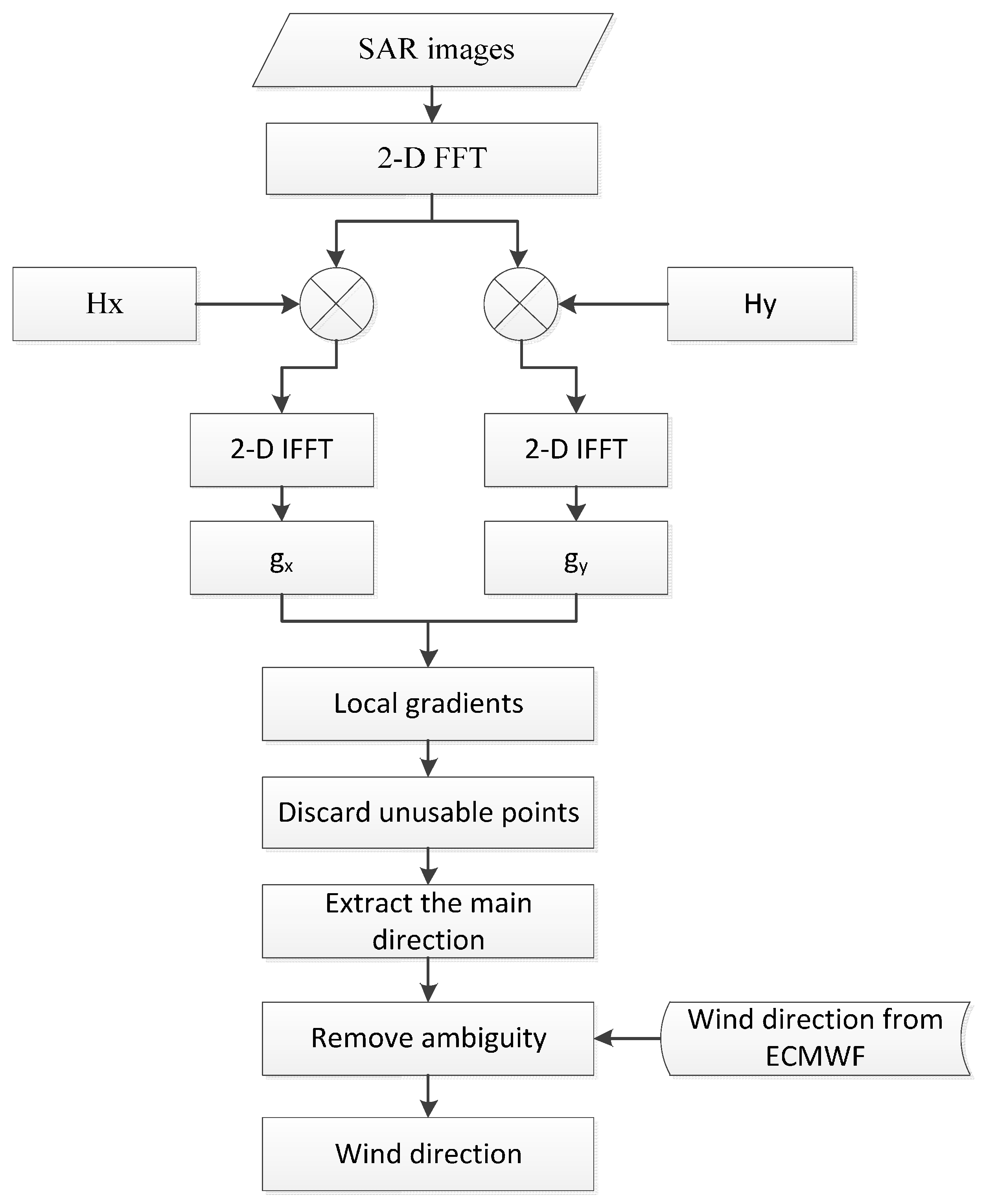
Figure 2.
(a) An Envisat advanced synthetic aperture radar (ASAR) image acquired at 02:06 on 14 October 2007 in VV polarization with a resolution of 75 m. (b) The subimage which is indicated by the red box in (a). White, red and green arrows indicate wind directions obtained from improved local gradients (ILG) method, European Centre for Medium-Range Weather Forecast (ECMWF) and Cross-Calibrated Multi-Platform (CCMP), respectively.

Figure 3.
The amplitude distributions of (a) and (b), σ is 15.
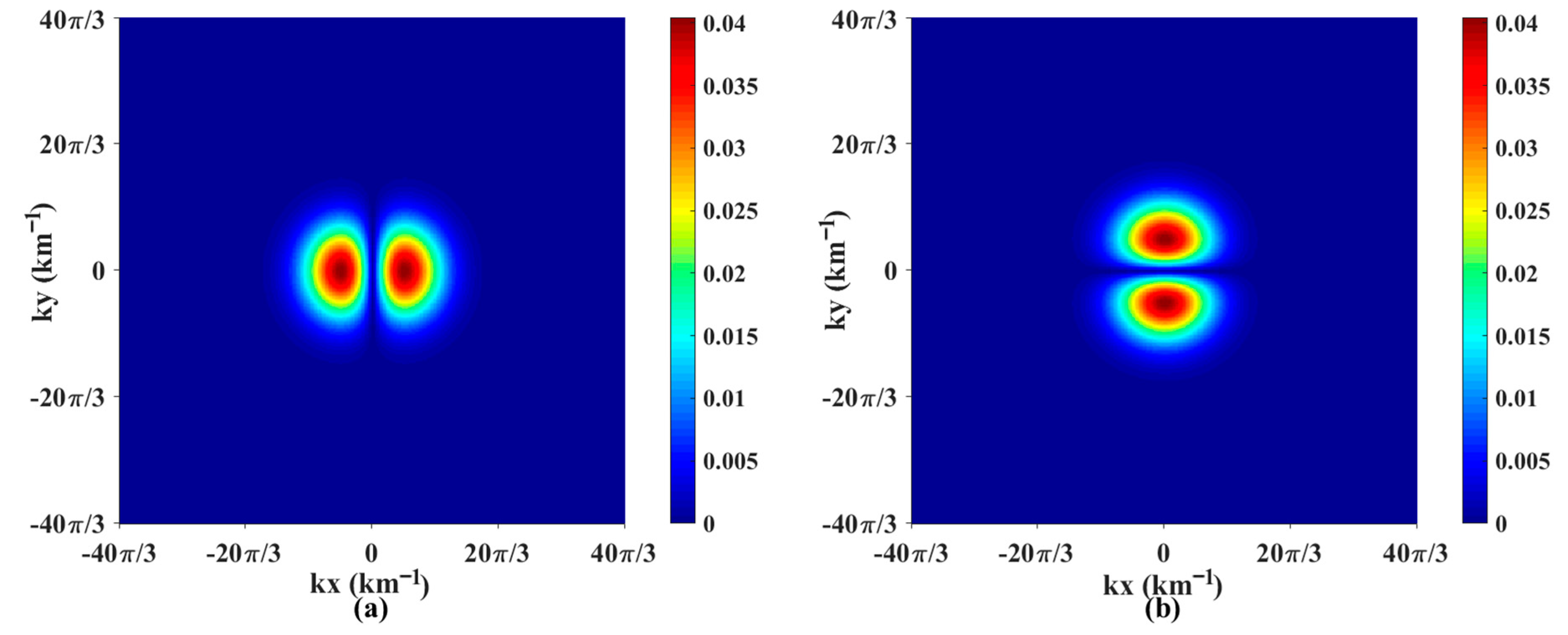
Figure 4.
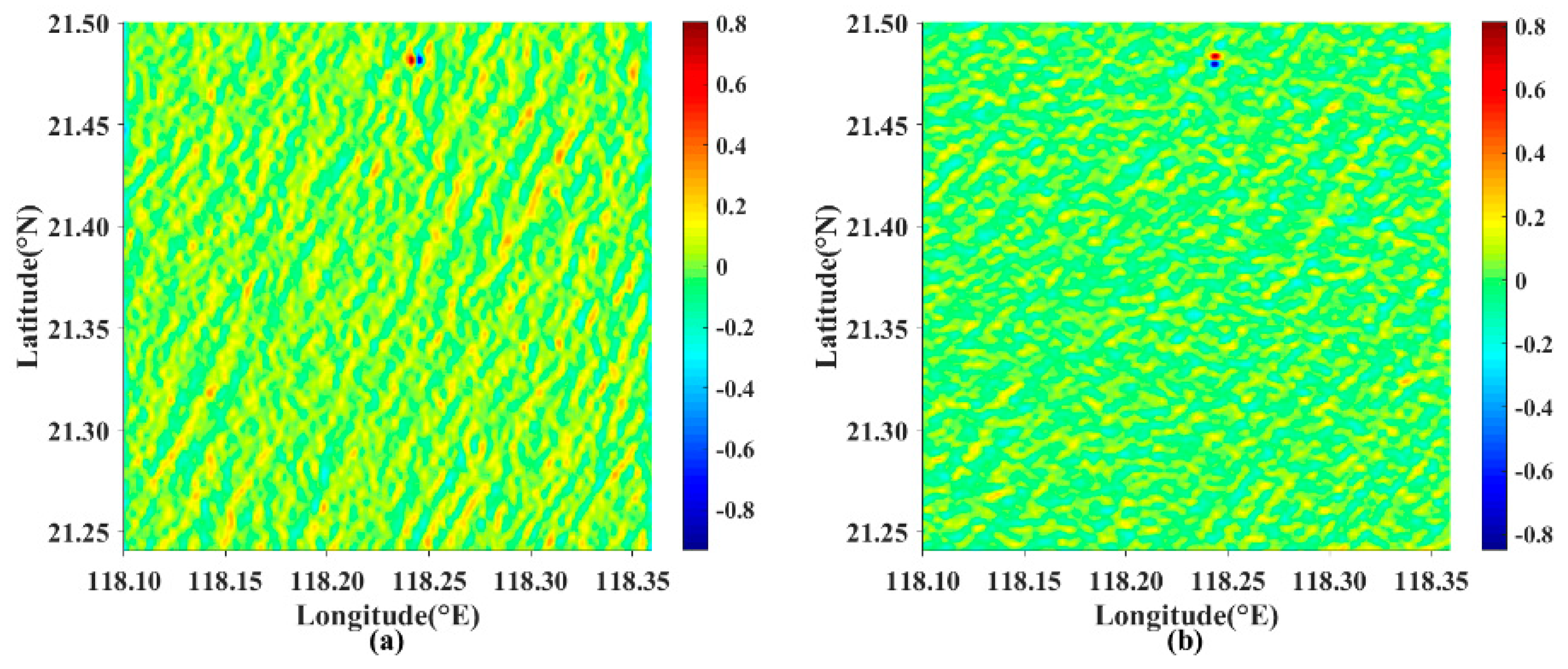
Computed (a) and (b) of the SAR image in Figure 2b.
Figure 4.
Computed (a) and (b) of the SAR image in Figure 2b.

Figure 5.
The distribution of wind directions of the images.

Figure 6.
Comparison of wind directions between each retrieval method and ECMWF: (a) fast Fourier transform (FFT)-like method, (b) local gradients (LG)-like method, (c) ILG method.
Figure 6.
Comparison of wind directions between each retrieval method and ECMWF: (a) fast Fourier transform (FFT)-like method, (b) local gradients (LG)-like method, (c) ILG method.
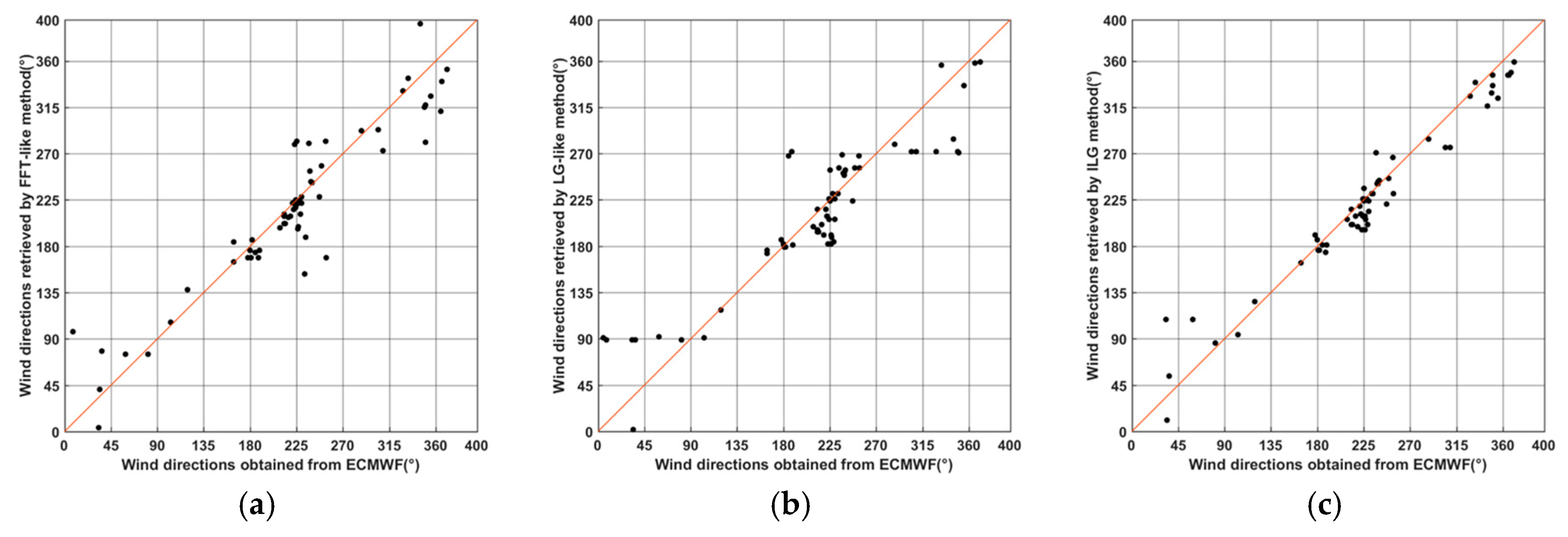
Figure 7.
Comparison of wind directions between each retrieval method and CCMP: (a) FFT-like method, (b) LG-like method and (c) ILG method.
Figure 7.
Comparison of wind directions between each retrieval method and CCMP: (a) FFT-like method, (b) LG-like method and (c) ILG method.
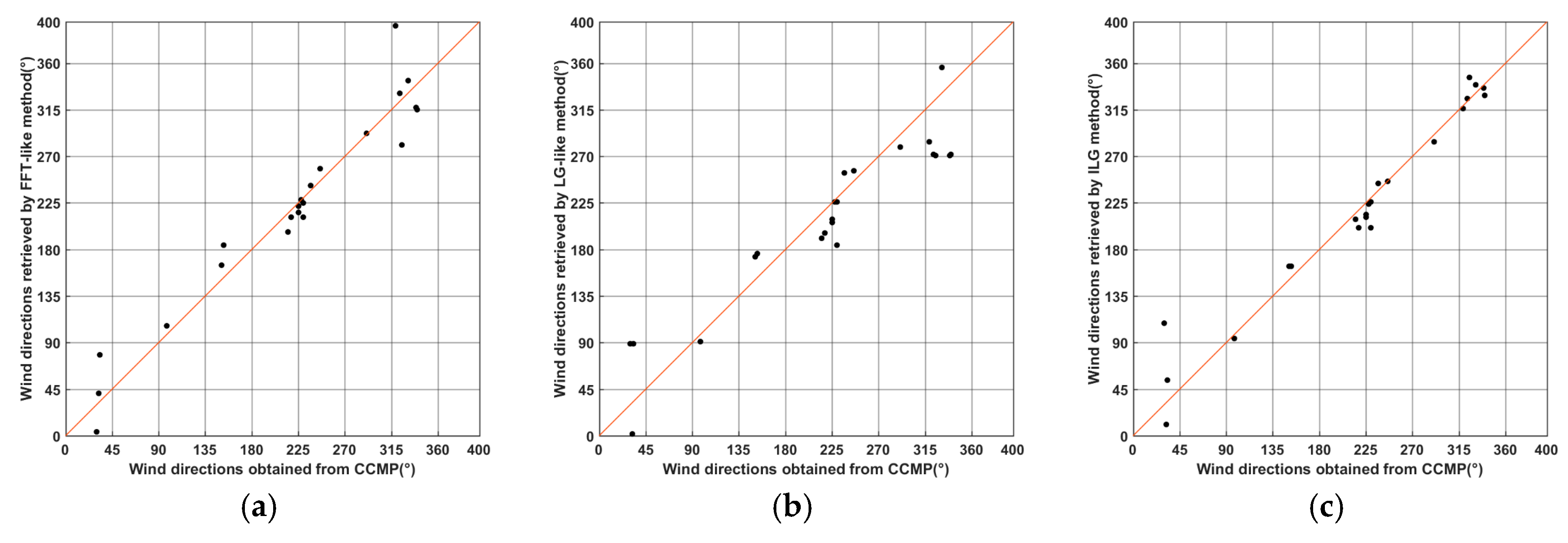
Figure 8.
Wind directions retrieved by the three methods from 75 m pixels on different grids of the ASAR image in Figure 2b: (a) 7.5 km grid, (b) 6 km grid, (c) 3 km grid. Yellow, magenta and cyan arrows indicate wind directions retrieved by the FFT-like, LG-like and ILG methods, respectively.
Figure 8.
Wind directions retrieved by the three methods from 75 m pixels on different grids of the ASAR image in Figure 2b: (a) 7.5 km grid, (b) 6 km grid, (c) 3 km grid. Yellow, magenta and cyan arrows indicate wind directions retrieved by the FFT-like, LG-like and ILG methods, respectively.

Figure 9.
Wind directions retrieved by the three methods on different grids of the ASAR image acquired at 00:45, 25 March 2005 in VV polarization: (a) 7.5 km grid, (b) 6 km grid, (c) 3 km grid. Yellow, magenta and cyan arrows indicate wind directions retrieved by the FFT-like, LG-like and ILG methods, respectively.
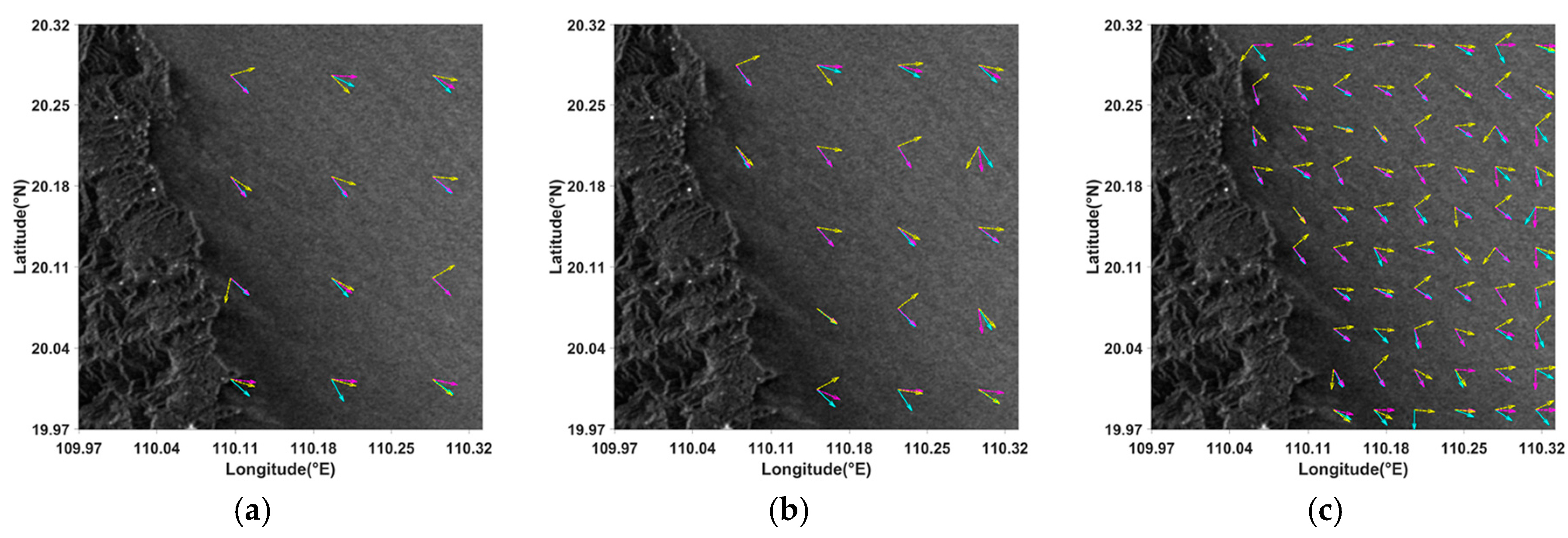
Figure 10.
Wind directions retrieved by the three methods on different grids of the Radarsat-2 image acquired at 17:58, 11 February 2011 in VV polarization: (a) 8 km grid, (b) 6.4 km grid, (c) 3.2 km grid. Yellow, magenta and cyan arrows indicate wind directions retrieved by the FFT-like, LG-like and ILG methods, respectively. The buoy (46073) is marked as the green dot and the in situ measurement is indicated by the green arrow.

Figure 11.
The image in Figure 2b is corrupted by each kind of noise: (a) salt-and-pepper noise (10% of contaminated pixels), (b) additive noise (SNR is −10 dB), (c) multiplicative noise (variance of n’ is 0.4), (d) speckle noise.
Figure 11.
The image in Figure 2b is corrupted by each kind of noise: (a) salt-and-pepper noise (10% of contaminated pixels), (b) additive noise (SNR is −10 dB), (c) multiplicative noise (variance of n’ is 0.4), (d) speckle noise.
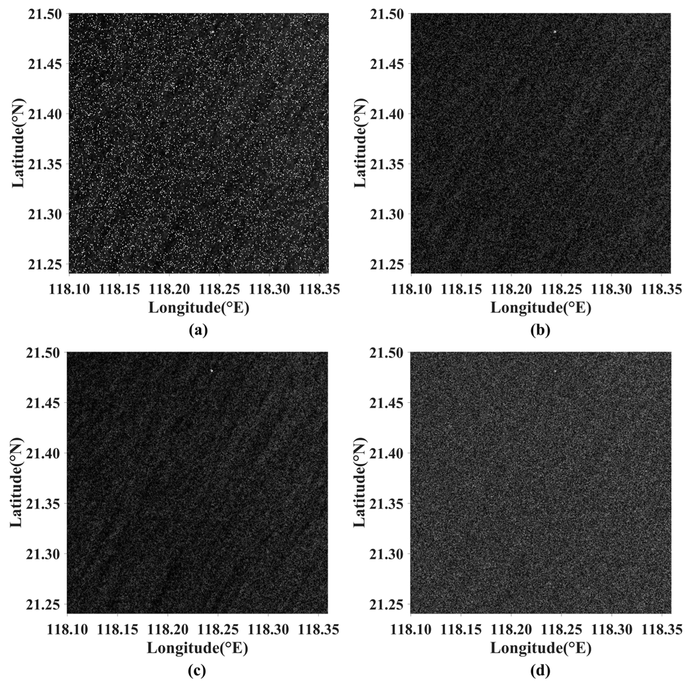
Figure 12.
Root-mean-square (RMS) differences between the retrieved results of each method and the interpolating wind directions when the salt-and-pepper noise exists with different intensity: (a) ECMWF and (b) CCMP.
Figure 12.
Root-mean-square (RMS) differences between the retrieved results of each method and the interpolating wind directions when the salt-and-pepper noise exists with different intensity: (a) ECMWF and (b) CCMP.

Figure 13.
RMS differences between the retrieved results of each method and the interpolating wind directions when the additive noise exists with a different signal-to-noise ratio (SNR): (a) ECMWF and (b) CCMP.
Figure 13.
RMS differences between the retrieved results of each method and the interpolating wind directions when the additive noise exists with a different signal-to-noise ratio (SNR): (a) ECMWF and (b) CCMP.

Figure 14.
RMS differences between the retrieved results of each method and the interpolating wind directions when the multiplicative noise exists with different variance: (a) ECMWF and (b) CCMP.
Figure 14.
RMS differences between the retrieved results of each method and the interpolating wind directions when the multiplicative noise exists with different variance: (a) ECMWF and (b) CCMP.


Table 1.
The results of general statistics between wind directions obtained by different retrieval methods and ECMWF reanalysis data for 62 images.
Table 1.
The results of general statistics between wind directions obtained by different retrieval methods and ECMWF reanalysis data for 62 images.
| FFT-Like Method | LG-Like Method | ILG Method | |
|---|---|---|---|
| RMS(°) | 30.22 | 36.10 | 21.57 |
| R | 0.9344 | 0.9314 | 0.9765 |
| p-value | 1.38 × 10⁻²⁸ | 4.30 × 10⁻²⁵ | 1.03 × 10−41 |
Table 2.
The results of general statistics between wind directions obtained by different retrieval methods and CCMP data for 22 images.
Table 2.
The results of general statistics between wind directions obtained by different retrieval methods and CCMP data for 22 images.
| FFT-Like Method | LG-Like Method | ILG Method | |
|---|---|---|---|
| RMS(°) | 25.41 | 36.65 | 21.61 |
| R | 0.9659 | 0.9413 | 0.9771 |
| p-value | 3.29 × 10⁻¹³ | 6.92 × 10⁻¹¹ | 6.55 × 10⁻¹⁵ |
Table 3.
The RMS differences between retrieved results of each method of the images corrupted by the speckle noise and wind directions obtained from the ECMWF (or CCMP) data.
Table 3.
The RMS differences between retrieved results of each method of the images corrupted by the speckle noise and wind directions obtained from the ECMWF (or CCMP) data.
| FFT-Like Method | LG-Like Method | ILG Method | |
|---|---|---|---|
| ECMWF | 46.73° | 45.29° | 37.06° |
| CCMP | 46.39° | 42.14° | 37.19° |
© 2017 by the authors. Licensee MDPI, Basel, Switzerland. This article is an open access article distributed under the terms and conditions of the Creative Commons Attribution (CC BY) license (http://creativecommons.org/licenses/by/4.0/).
Share and Cite
MDPI and ACS Style
Zhou, L.; Zheng, G.; Li, X.; Yang, J.; Ren, L.; Chen, P.; Zhang, H.; Lou, X. An Improved Local Gradient Method for Sea Surface Wind Direction Retrieval from SAR Imagery. Remote Sens. 2017, 9, 671. https://doi.org/10.3390/rs9070671
AMA Style
Zhou L, Zheng G, Li X, Yang J, Ren L, Chen P, Zhang H, Lou X. An Improved Local Gradient Method for Sea Surface Wind Direction Retrieval from SAR Imagery. Remote Sensing. 2017; 9(7):671. https://doi.org/10.3390/rs9070671
Chicago/Turabian StyleZhou, Lizhang, Gang Zheng, Xiaofeng Li, Jingsong Yang, Lin Ren, Peng Chen, Huaguo Zhang, and Xiulin Lou. 2017. "An Improved Local Gradient Method for Sea Surface Wind Direction Retrieval from SAR Imagery" Remote Sensing 9, no. 7: 671. https://doi.org/10.3390/rs9070671
Note that from the first issue of 2016, this journal uses article numbers instead of page numbers. See further details here.