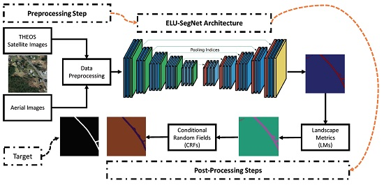
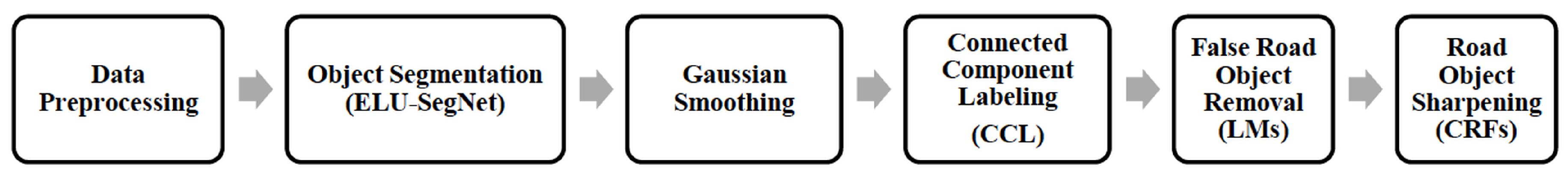
Figure 1.
A process in our proposed framework.
Figure 1.
A process in our proposed framework.
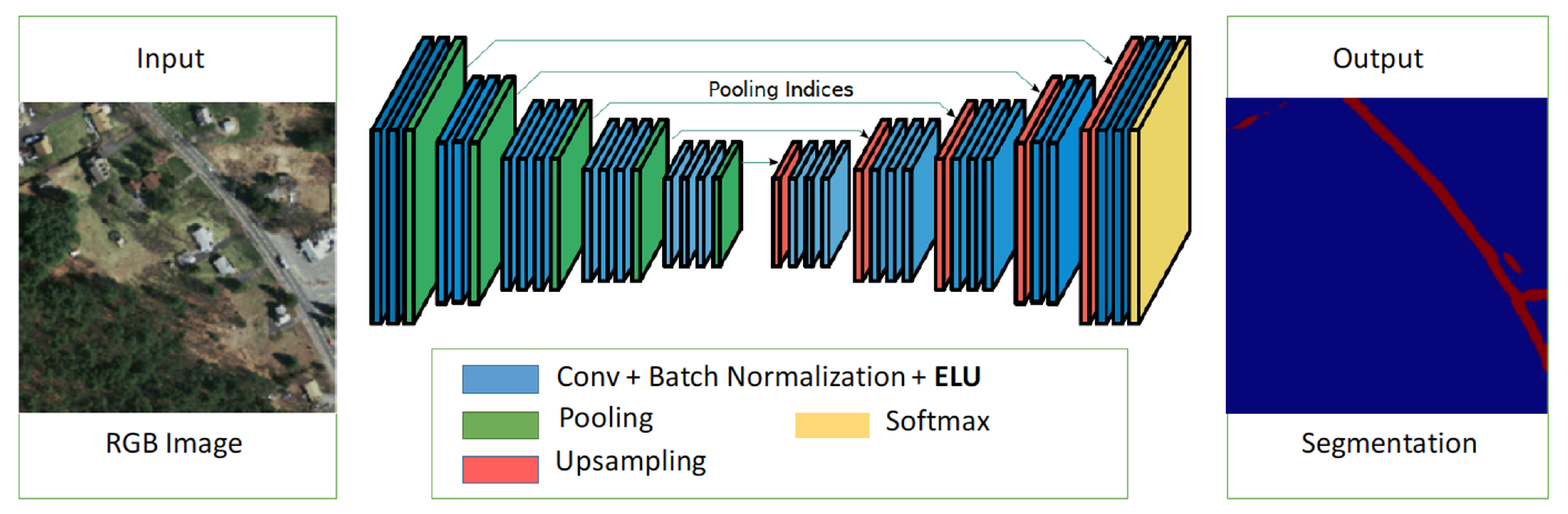
Figure 2.
A proposed network architecture for object segmentation (exponential linear unit (ELU)-SegNet).
Figure 2.
A proposed network architecture for object segmentation (exponential linear unit (ELU)-SegNet).
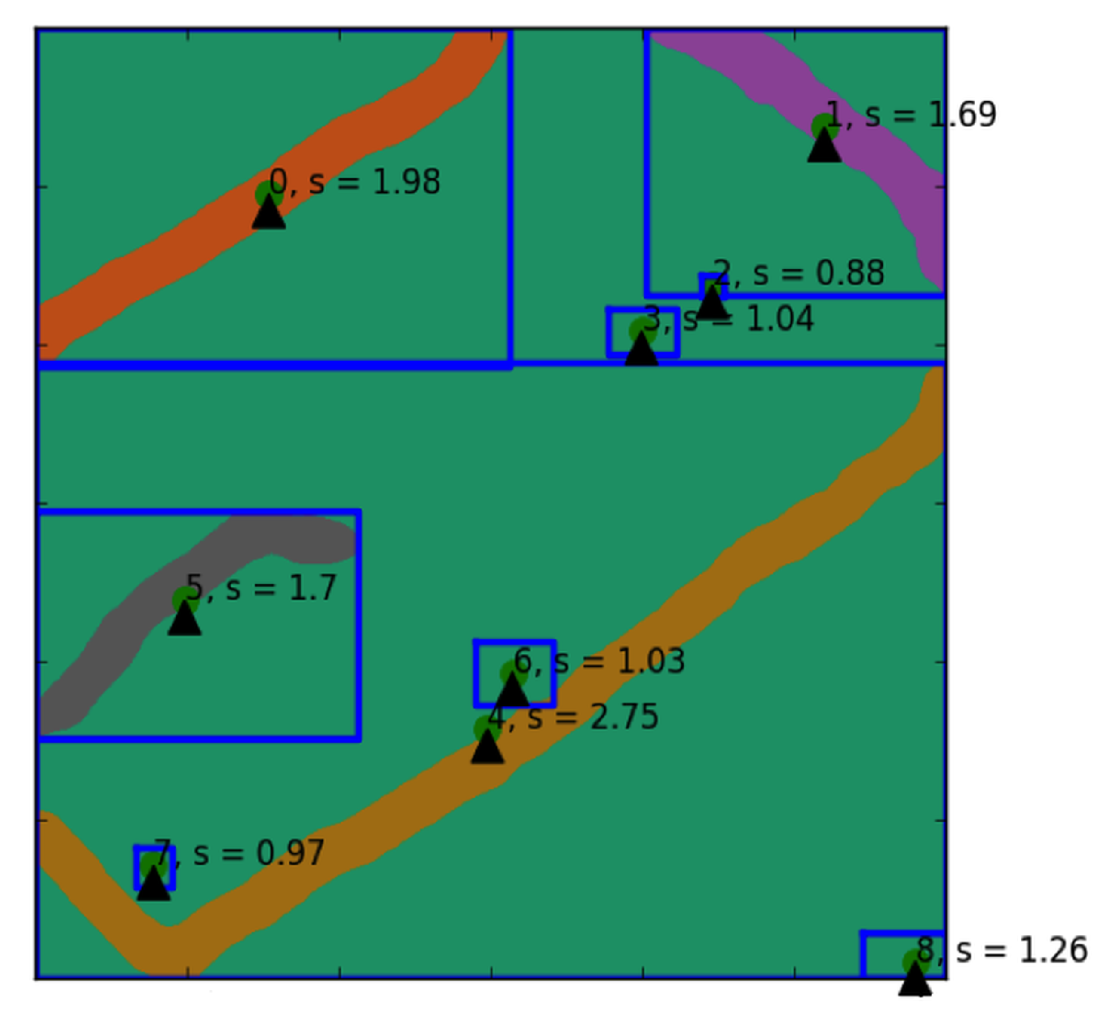
Figure 3.
Illustration of shape index scores on each extracted road object. Any objects with shape index score lower than 1.25 are considered as noises and subsequently removed.
Figure 3.
Illustration of shape index scores on each extracted road object. Any objects with shape index score lower than 1.25 are considered as noises and subsequently removed.
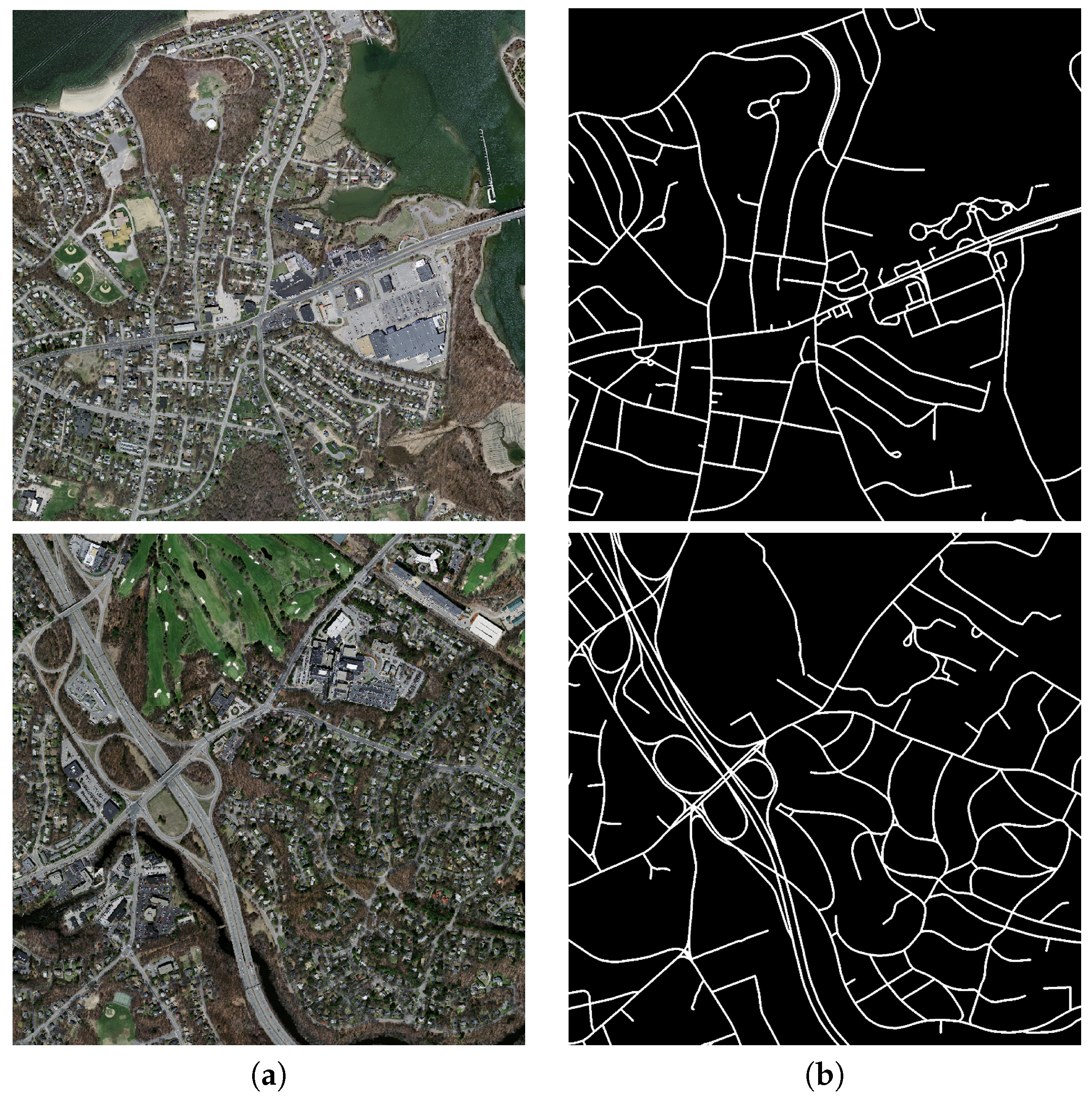
Figure 4.
Two sample aerial images from the Massachusetts road corpus, where a row refers to each image (a) Aerial image and (b) Binary map, which is a ground truth image denoting the location of roads.
Figure 4.
Two sample aerial images from the Massachusetts road corpus, where a row refers to each image (a) Aerial image and (b) Binary map, which is a ground truth image denoting the location of roads.
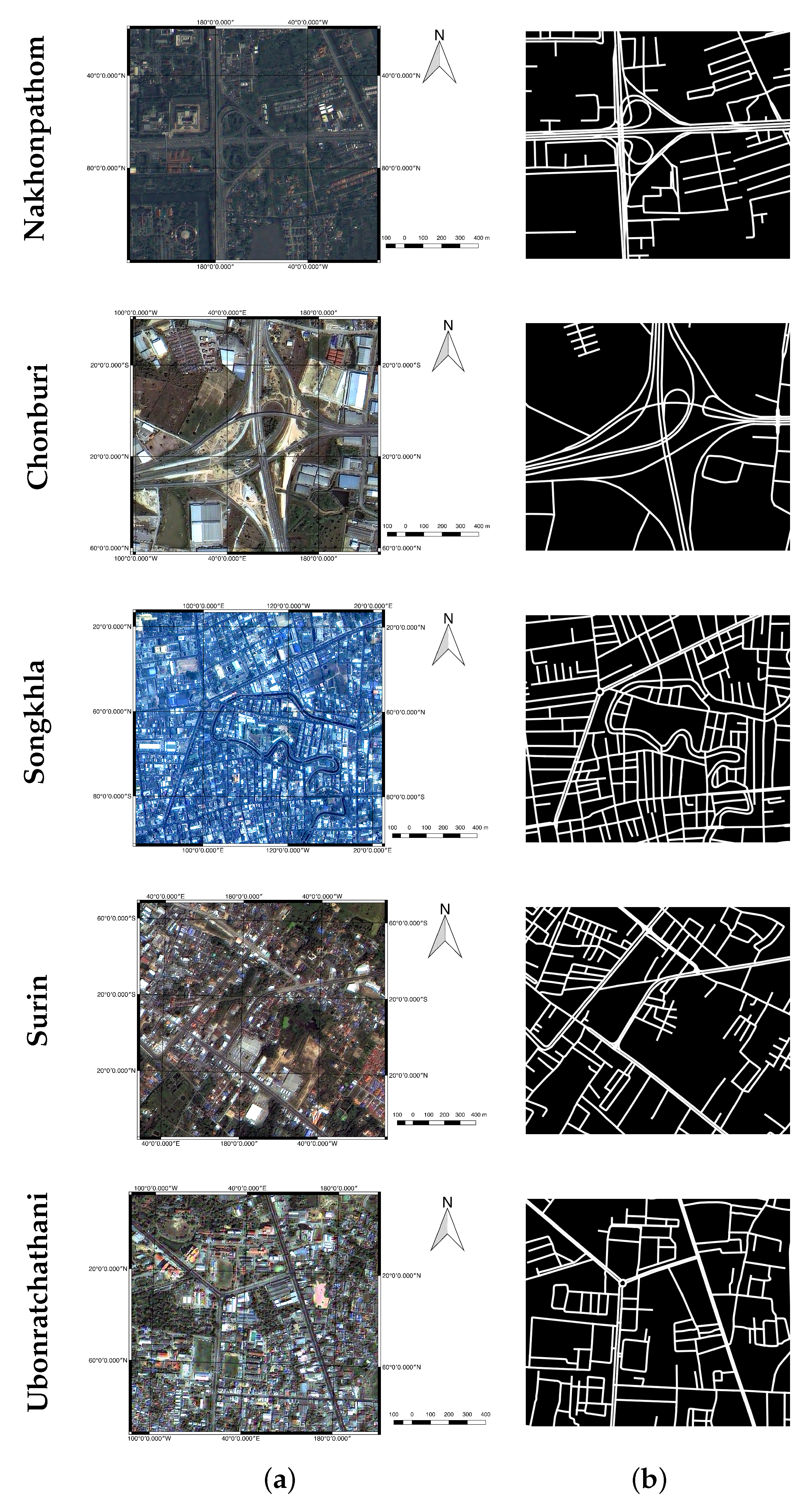
Figure 5.
Sample satellite images from five provinces of our data sets; each row refers to a single sample image from one province (Nakhonpathom, Chonburi, Songkhla, Surin, and Ubonratchathani) in a satellite image format (a) and in a binary map (b), which is served as a ground truth image denoting the location of roads.
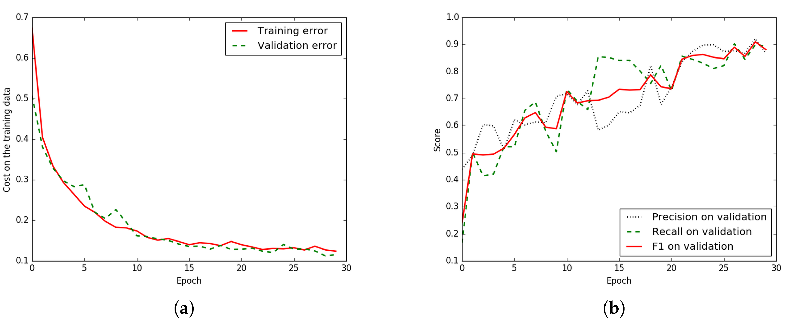
Figure 6.
Iteration plot on Massachusetts aerial corpus of the proposed technique, ELU-SegNet-LMs-CRFs; x refers to epochs and y refers to different measures. (a) Plot of model loss (cross entropy) on training and validation data sets, and (b) Performance plot on the validation data set.
Figure 6.
Iteration plot on Massachusetts aerial corpus of the proposed technique, ELU-SegNet-LMs-CRFs; x refers to epochs and y refers to different measures. (a) Plot of model loss (cross entropy) on training and validation data sets, and (b) Performance plot on the validation data set.
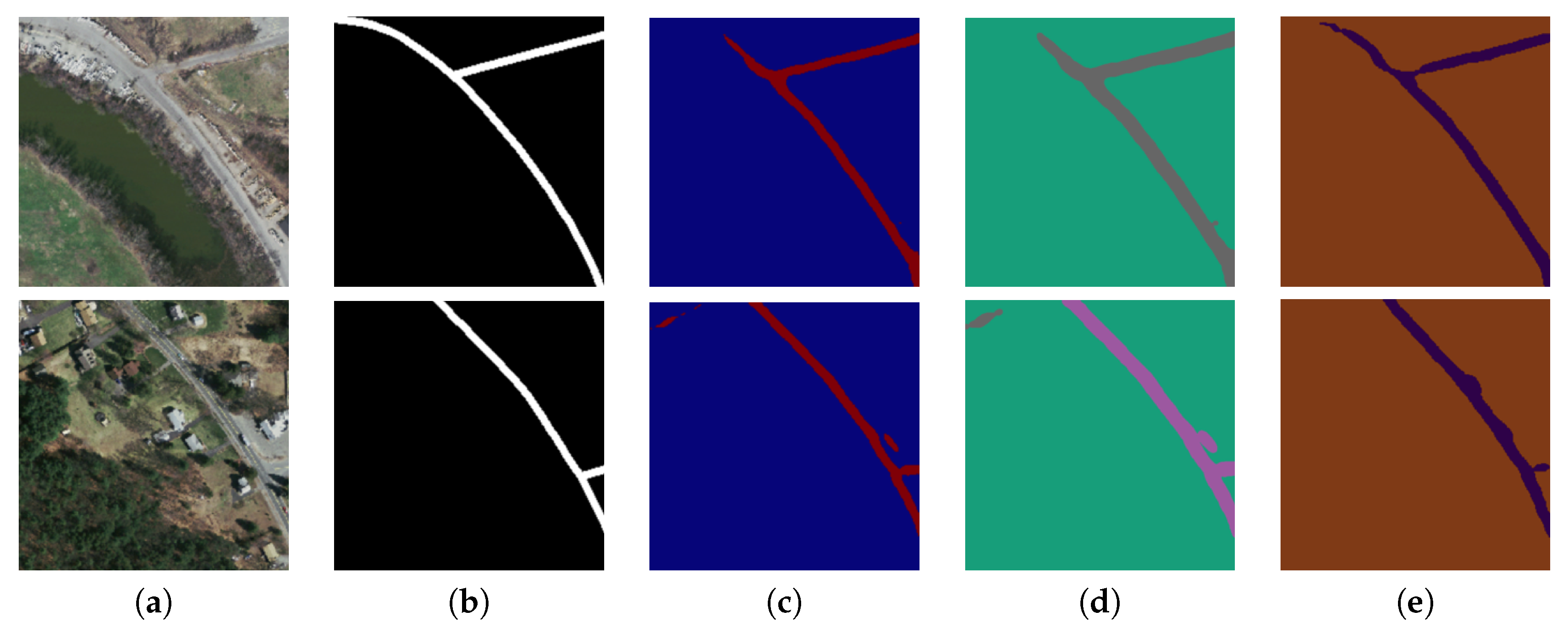
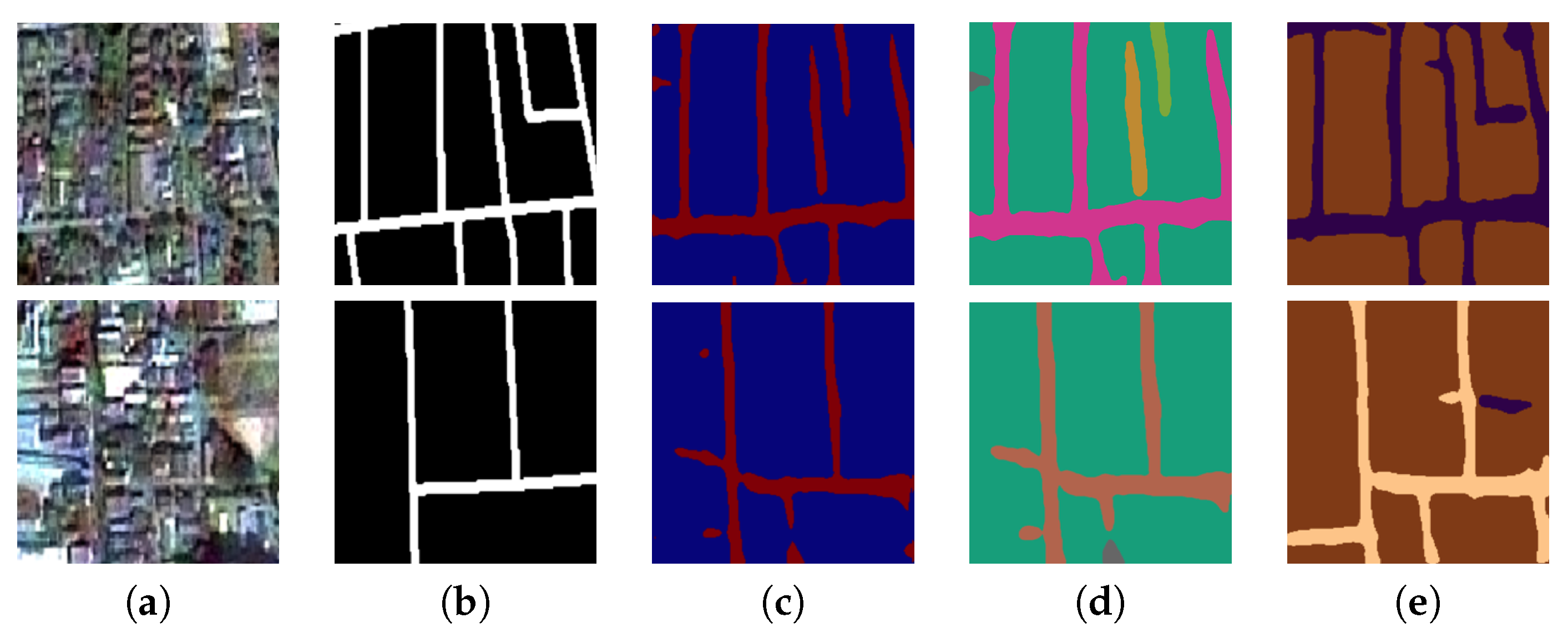
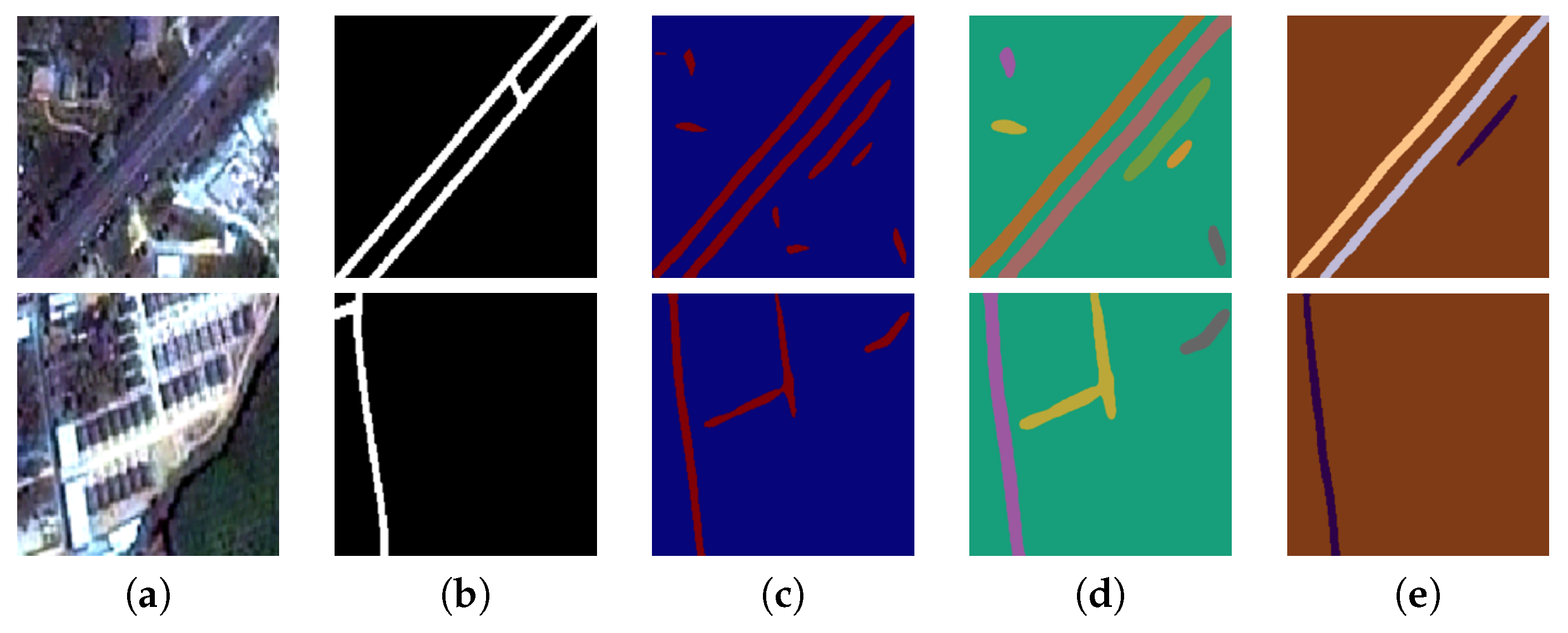
Figure 7.
Two sample input and output aerial images on Massachusetts corpus, where rows refer different images. (a) Original input image; (b) Target road map (ground truth); (c) Output of ELU-SegNet; (d) Output of ELU-SegNet-LMs; and (e) Output of ELU-SegNet-LMs-CRFs.
Figure 7.
Two sample input and output aerial images on Massachusetts corpus, where rows refer different images. (a) Original input image; (b) Target road map (ground truth); (c) Output of ELU-SegNet; (d) Output of ELU-SegNet-LMs; and (e) Output of ELU-SegNet-LMs-CRFs.
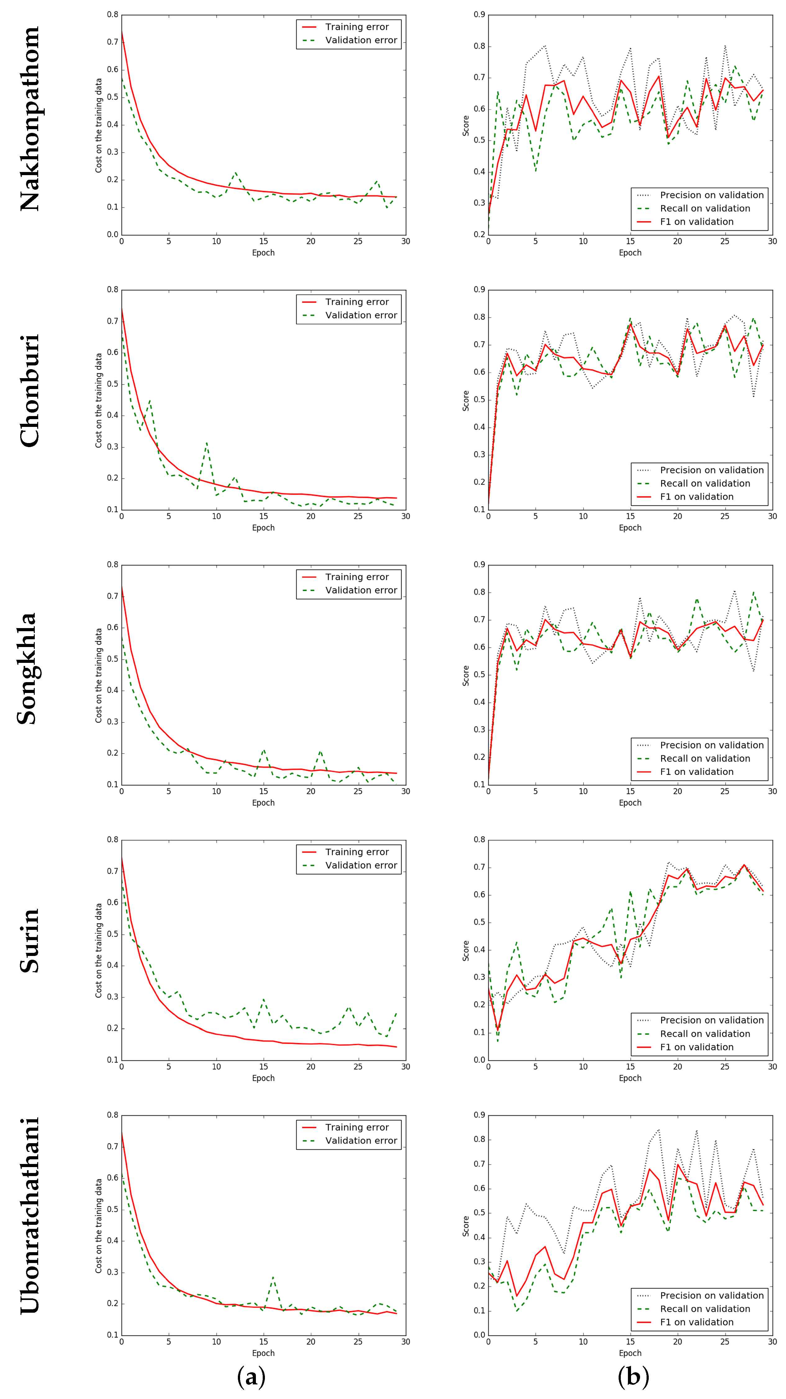
Figure 8.
Iteration plot on THEOS satellite data sets of the proposed technique, ELU-SegNet-LMs-CRFs. x refers to epochs and y refers to different measures. Each row refers to different data set (province). (a) Plot of model loss (cross entropy) on training and validation data sets; and (b) Performance plot on the validation data set.
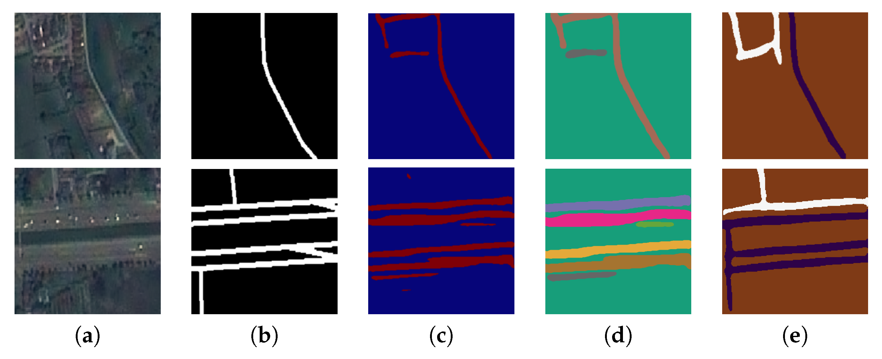
Figure 9.
Two sample input and output THEOS satellite images on the Nakhonpathom data set, where rows refer different images. (a) Original input image; (b) Target road map (ground truth); (c) Output of ELU-SegNet; (d) Output of ELU-SegNet-LMs; and (e) Output of ELU-SegNet-LMs-CRFs.
Figure 9.
Two sample input and output THEOS satellite images on the Nakhonpathom data set, where rows refer different images. (a) Original input image; (b) Target road map (ground truth); (c) Output of ELU-SegNet; (d) Output of ELU-SegNet-LMs; and (e) Output of ELU-SegNet-LMs-CRFs.
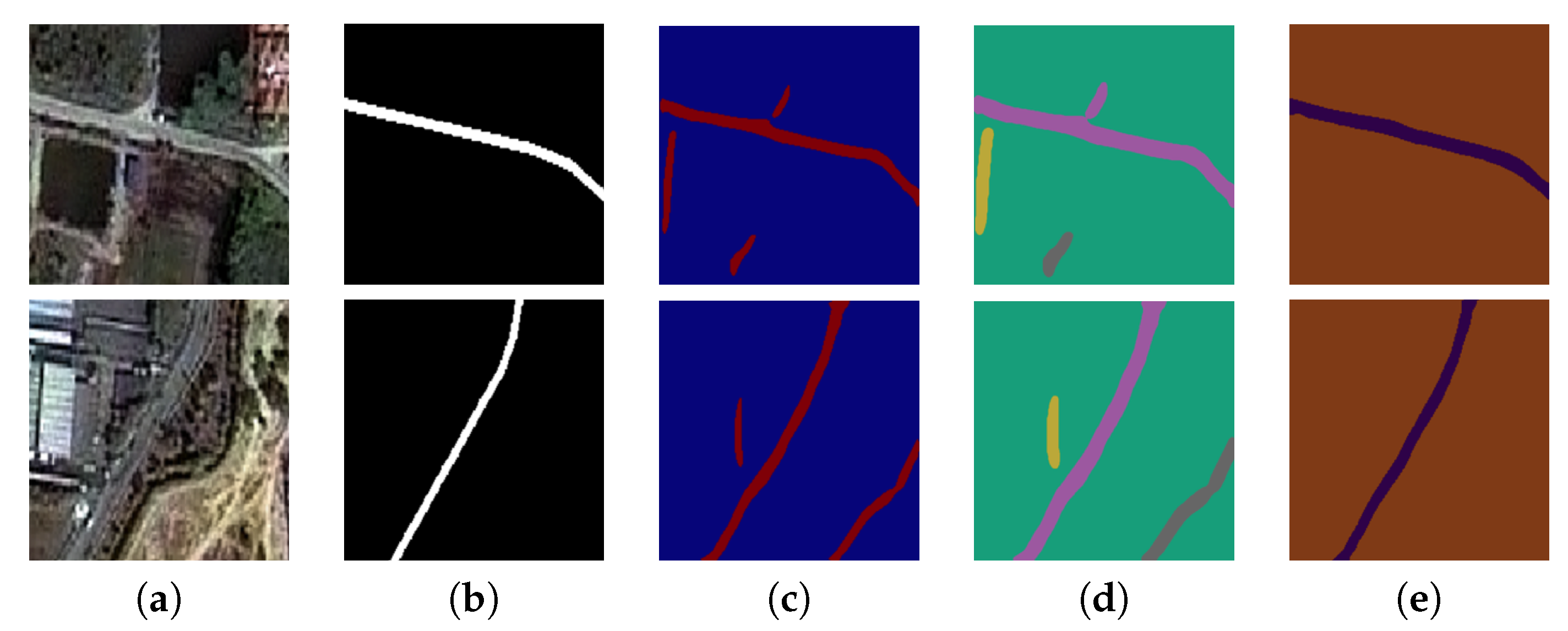
Figure 10.
Two sample input and output THEOS satellite images on the Chonburi data set, where rows refer different images. (a) Original input image; (b) Target road map (ground truth); (c) Output of ELU-SegNet; (d) Output of ELU-SegNet-LMs; and (e) Output of ELU-SegNet-LMs-CRFs.
Figure 10.
Two sample input and output THEOS satellite images on the Chonburi data set, where rows refer different images. (a) Original input image; (b) Target road map (ground truth); (c) Output of ELU-SegNet; (d) Output of ELU-SegNet-LMs; and (e) Output of ELU-SegNet-LMs-CRFs.
Figure 11.
Two sample input and output THEOS satellite images on the Songkhla data set, where rows refer different images. (a) Original input image; (b) Target road map (ground truth); (c) Output of ELU-SegNet; (d) Output of ELU-SegNet-LMs; and (e) Output of ELU-SegNet-LMs-CRFs.
Figure 11.
Two sample input and output THEOS satellite images on the Songkhla data set, where rows refer different images. (a) Original input image; (b) Target road map (ground truth); (c) Output of ELU-SegNet; (d) Output of ELU-SegNet-LMs; and (e) Output of ELU-SegNet-LMs-CRFs.
Figure 12.
Two sample input and output THEOS satellite images on the Surin data set, where rows refer different images. (a) Original input image; (b) Target road map (ground truth); (c) Output of ELU-SegNet; (d) output of ELU-SegNet-LMs; and (e) Output of ELU-SegNet-LMs-CRFs.
Figure 12.
Two sample input and output THEOS satellite images on the Surin data set, where rows refer different images. (a) Original input image; (b) Target road map (ground truth); (c) Output of ELU-SegNet; (d) output of ELU-SegNet-LMs; and (e) Output of ELU-SegNet-LMs-CRFs.
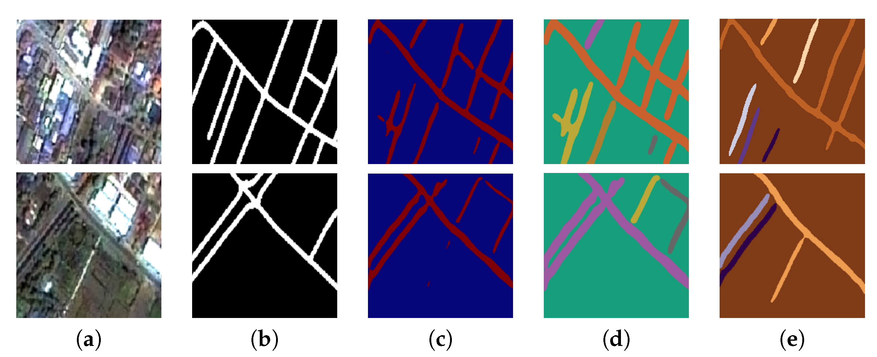
Figure 13.
Two sample input and output THEOS satellite images on Ubonratchathani data set, where rows refer different images. (a) Original input image; (b) Target road map (ground truth); (c) Output of ELU-SegNet; (d) Output of ELU-SegNet-LMs; and (e) Output of ELU-SegNet-LMs-CRFs.
Figure 13.
Two sample input and output THEOS satellite images on Ubonratchathani data set, where rows refer different images. (a) Original input image; (b) Target road map (ground truth); (c) Output of ELU-SegNet; (d) Output of ELU-SegNet-LMs; and (e) Output of ELU-SegNet-LMs-CRFs.
Table 1.
Numbers of training, validation, and testing sets.
Table 1.
Numbers of training, validation, and testing sets.
| | Training Set | Validation Set | Testing Set |
|---|
| Massachusetts | 1108 | 14 | 49 |
| Nakhonpathom | 200 | 14 | 49 |
| Chonburi | 100 | 14 | 49 |
| Songkhla | 100 | 14 | 49 |
| Surin | 70 | 14 | 49 |
| Ubonratchathani | 70 | 14 | 49 |
Table 2.
Variations of our proposed deep learning methods. LM: landscape metric; CRF: conditional random field.
Table 2.
Variations of our proposed deep learning methods. LM: landscape metric; CRF: conditional random field.
| Abbreviation | Description |
|---|
| ELU-SegNet | SegNet + ELU activation |
| ELU-SegNet-LMs | SegNet + ELU activation + Landscape Metrics |
| ELU-SegNet-LMs-CRFs | SegNet + ELU activation + Landscape Metrics + CRFs |
Table 3.
Results on the testing data of Massachusetts aerial corpus between four baselines and three variations of our proposed techniques in terms of , , and . FCN: fully convolutional network.
Table 3.
Results on the testing data of Massachusetts aerial corpus between four baselines and three variations of our proposed techniques in terms of , , and . FCN: fully convolutional network.
| | Model | Precsion | Recall | F1 |
|---|
| Baselines | Basic-model [2] | 0.657 | 0.657 | 0.657 |
| FCN-no-skip [2] | 0.742 | 0.742 | 0.742 |
| FCN-8s [2] | 0.762 | 0.762 | 0.762 |
| SegNet | 0.773 | 0.765 | 0.768 |
| Proposed Method | ELU-SegNet | 0.852 | 0.733 | 0.788 |
| ELU-SegNet-LMs | 0.854 | 0.861 | 0.857 |
| ELU-SegNet-LMs-CRFs | 0.858 | 0.894 | 0.876 |
Table 4.
on the testing data of the Thailand Earth Observation System (THEOS) satellite data sets between baseline (SegNet) and three variations of our proposed techniques; columns refer to five different provinces (data sets).
Table 4.
on the testing data of the Thailand Earth Observation System (THEOS) satellite data sets between baseline (SegNet) and three variations of our proposed techniques; columns refer to five different provinces (data sets).
| | Model | Nakhon. | Chonburi | Songkhla | Surin | Ubon. | Avg. |
|---|
| Baseline | SegNet | 0.422 | 0.572 | 0.424 | 0.501 | 0.406 | 0.465 |
| Proposed Method | ELU-SegNet | 0.463 | 0.690 | 0.497 | 0.591 | 0.534 | 0.555 |
| ELU-SegNet-LMs | 0.488 | 0.732 | 0.526 | 0.625 | 0.562 | 0.587 |
| ELU-SegNet-LMs-CRFs | 0.550 | 0.775 | 0.607 | 0.707 | 0.608 | 0.649 |
Table 5.
on the testing data of THEOS satellite data sets between baseline (SegNet) and three variations of our proposed techniques; columns refer to five different provinces (data sets).
Table 5.
on the testing data of THEOS satellite data sets between baseline (SegNet) and three variations of our proposed techniques; columns refer to five different provinces (data sets).
| | Model | Nakhon. | Chonburi | Songkhla | Surin | Ubon. | Avg. |
|---|
| Baseline | SegNet | 0.435 | 0.668 | 0.456 | 0.598 | 0.601 | 0.552 |
| Proposed Method | ELU-SegNet | 0.410 | 0.702 | 0.478 | 0.840 | 0.852 | 0.656 |
| ELU-SegNet-LMs | 0.494 | 0.852 | 0.557 | 0.770 | 0.867 | 0.708 |
| ELU-SegNet-LMs-CRFs | 0.535 | 0.909 | 0.650 | 0.786 | 0.871 | 0.751 |
Table 6.
on the testing data of THEOS satellite data sets between baseline (SegNet) and three variations of our proposed techniques; columns refer to five different provinces (data sets).
Table 6.
on the testing data of THEOS satellite data sets between baseline (SegNet) and three variations of our proposed techniques; columns refer to five different provinces (data sets).
| | Model | Nakhon. | Chonburi | Songkhla | Surin | Ubon. | Avg. |
|---|
| Baseline | SegNet | 0.410 | 0.499 | 0.395 | 0.431 | 0.306 | 0.408 |
| Proposed Method | ELU-SegNet | 0.532 | 0.678 | 0.517 | 0.456 | 0.389 | 0.515 |
| ELU-SegNet-LMs | 0.483 | 0.642 | 0.498 | 0.526 | 0.416 | 0.513 |
| ELU-SegNet-LMs-CRFs | 0.566 | 0.676 | 0.570 | 0.643 | 0.467 | 0.584 |


