
Remote Sensing of Spatiotemporal Changes in Wetland Geomorphology Based on Type 2 Fuzzy Sets: A Case Study of Beidagang Wetland from 1975 to 2015


Abstract
:1. Introduction
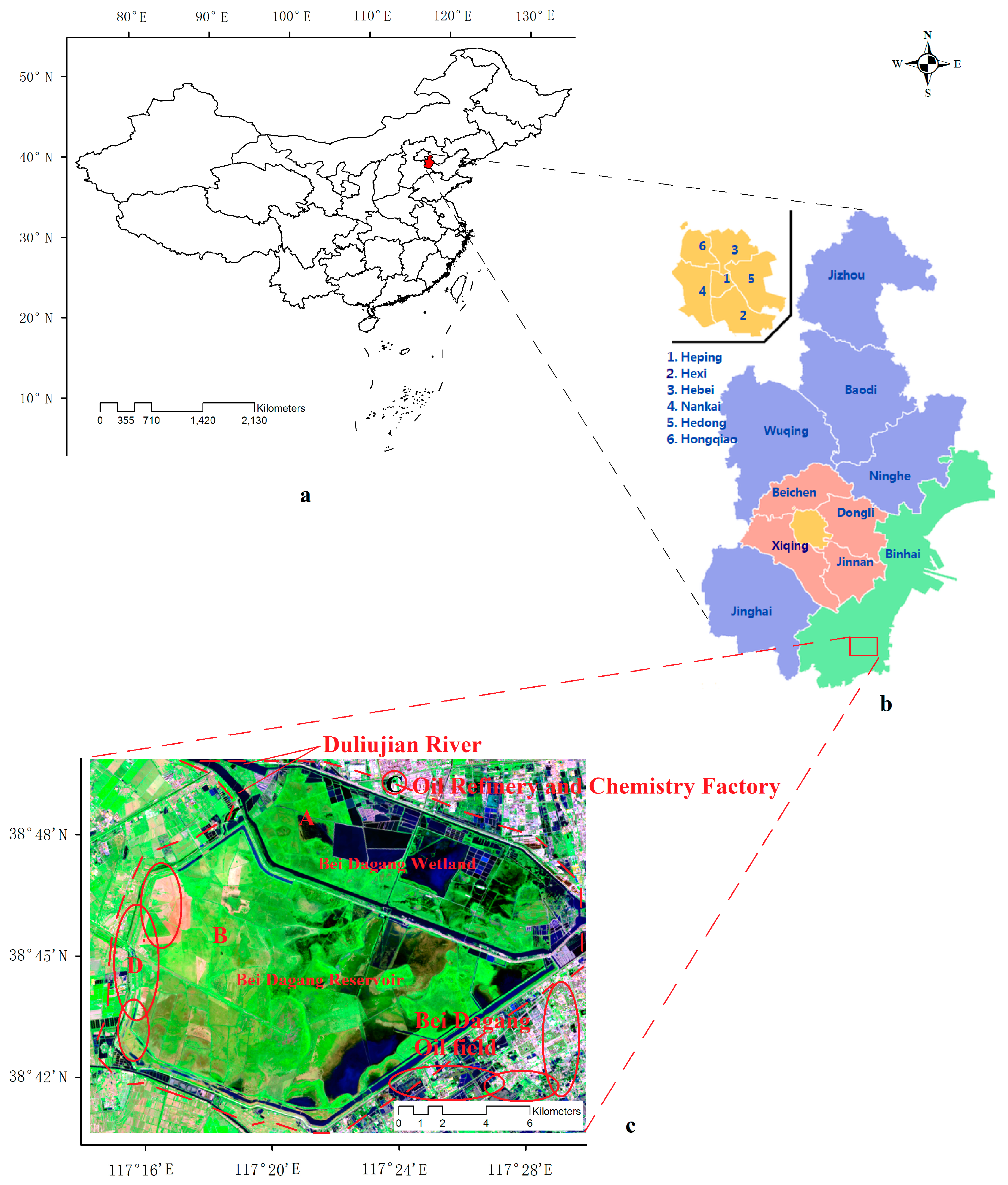
2. Study Area
3. Datasets and Preprocessing
3.1. EO-1 ALI Dataset
3.2. Sentinel-2 Dataset
3.3. Landsat Dataset
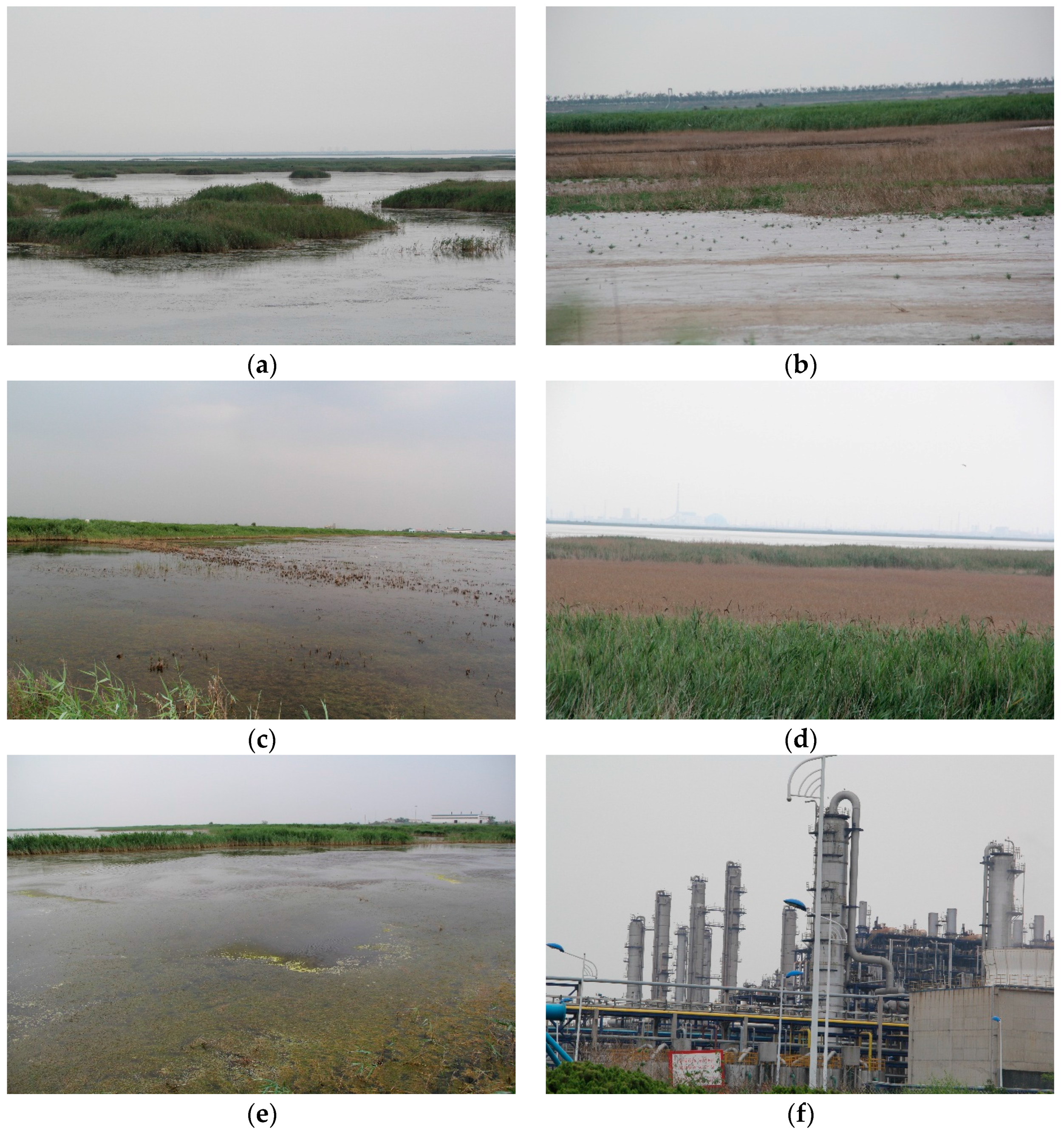
3.4. Field Survey Dataset
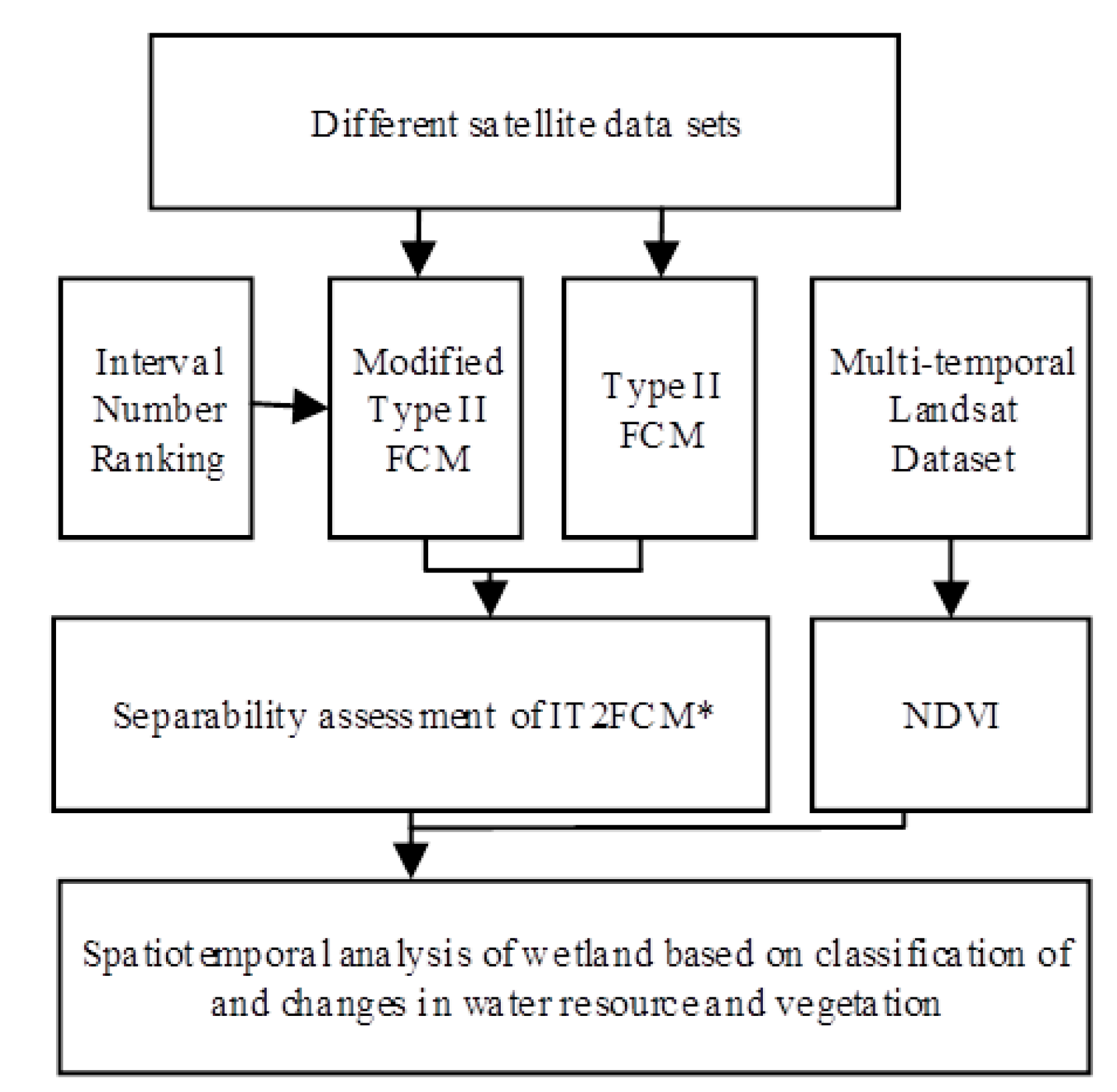
4. Methodology
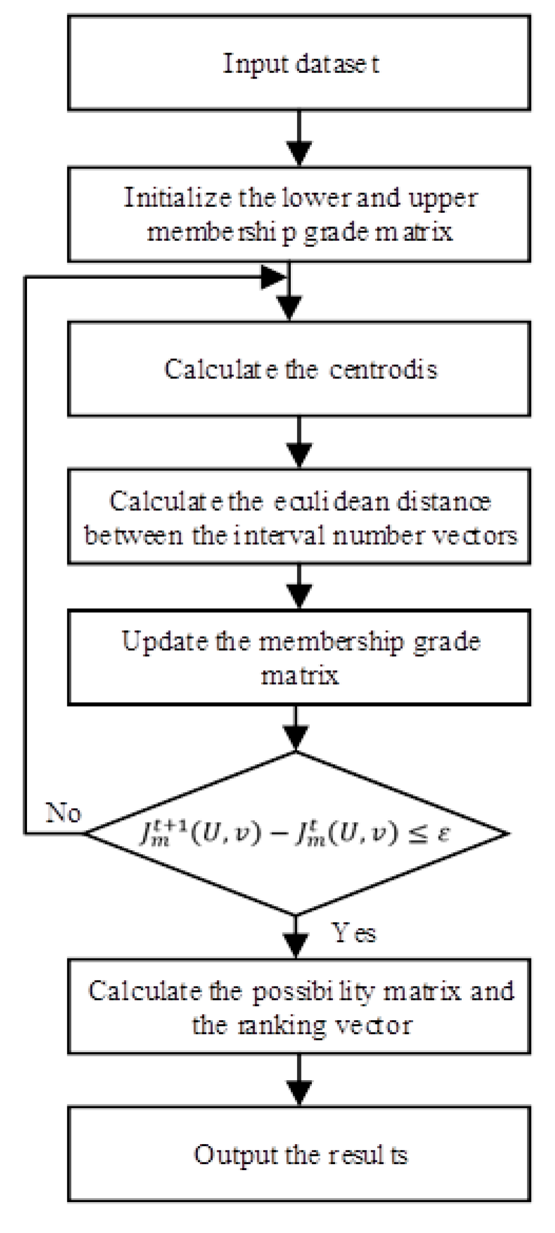
4.1. Introduction of IT2FCM
4.2. IT2FCM* Algorithm
4.3. Introduction of Four Validity Indexes
4.4. Vegetation Index
5. Experimental Results and Discussion
5.1. Separability Assessment Based on Four Validity Indexes for the Modified IT2FCM* Algorithm
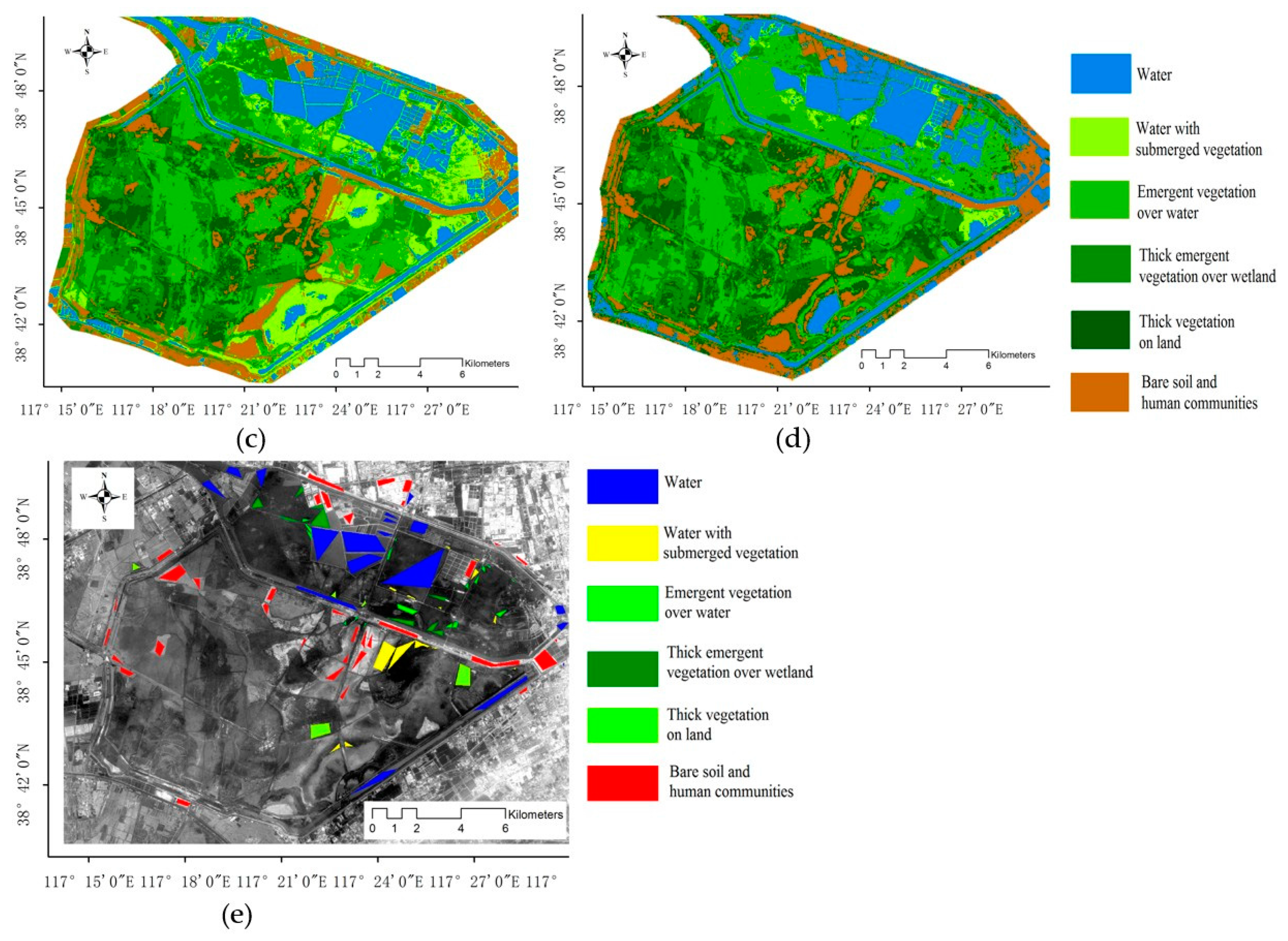
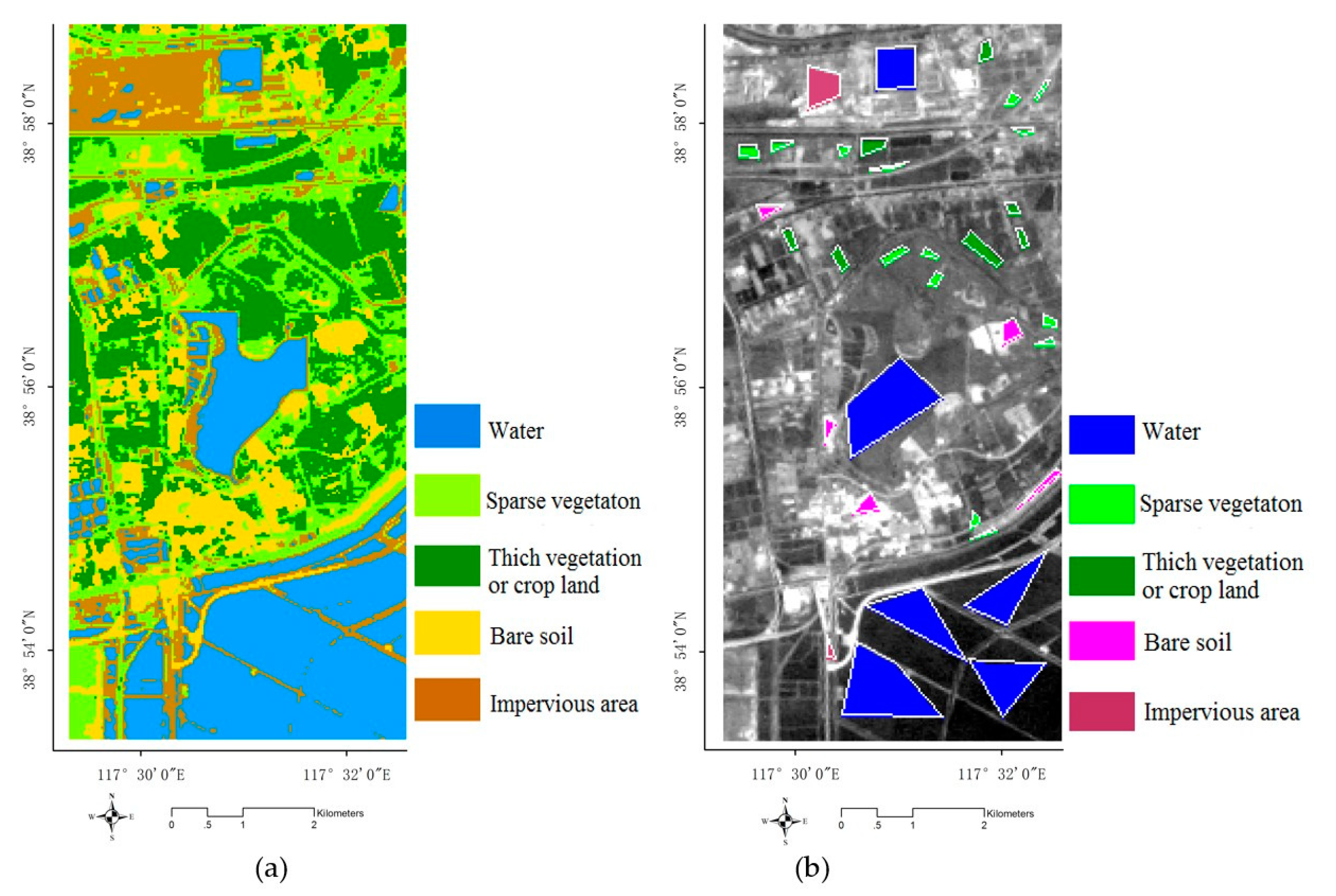
5.2. Separability Assessment Based on Accuracy of the Classification Results
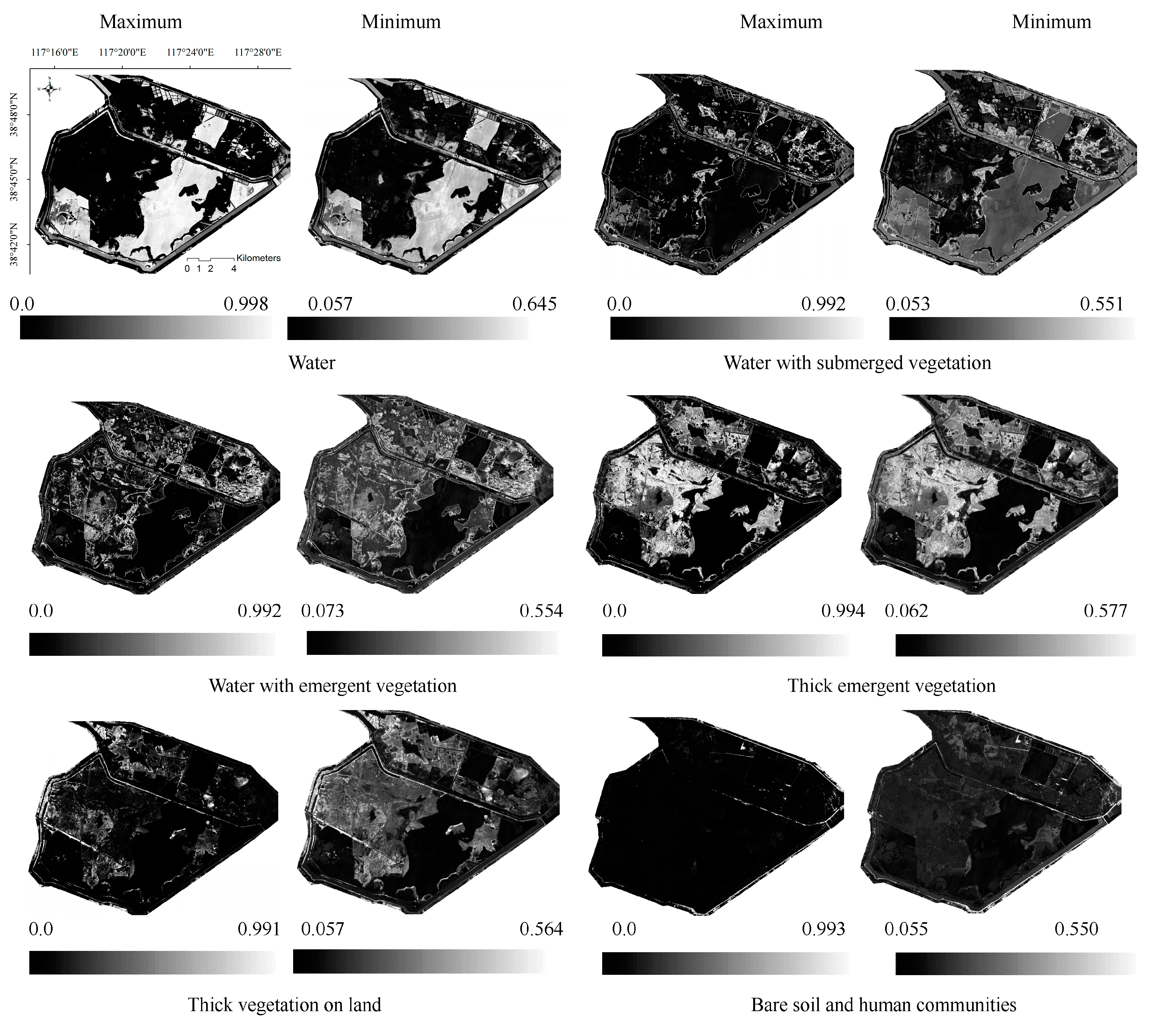
5.3. Separability Assessment Based on Analysis of the Membership of Classified Land Cover Types
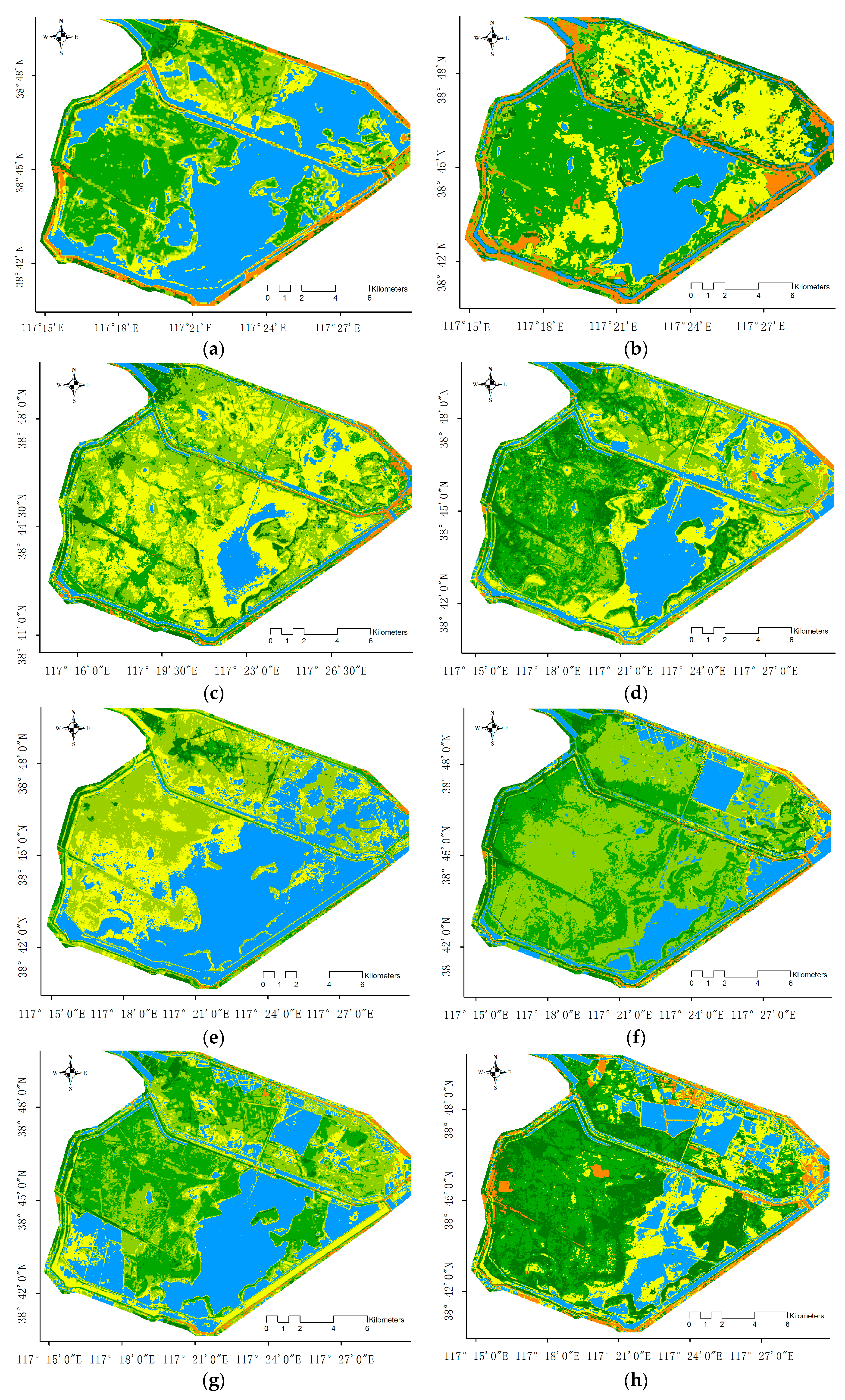
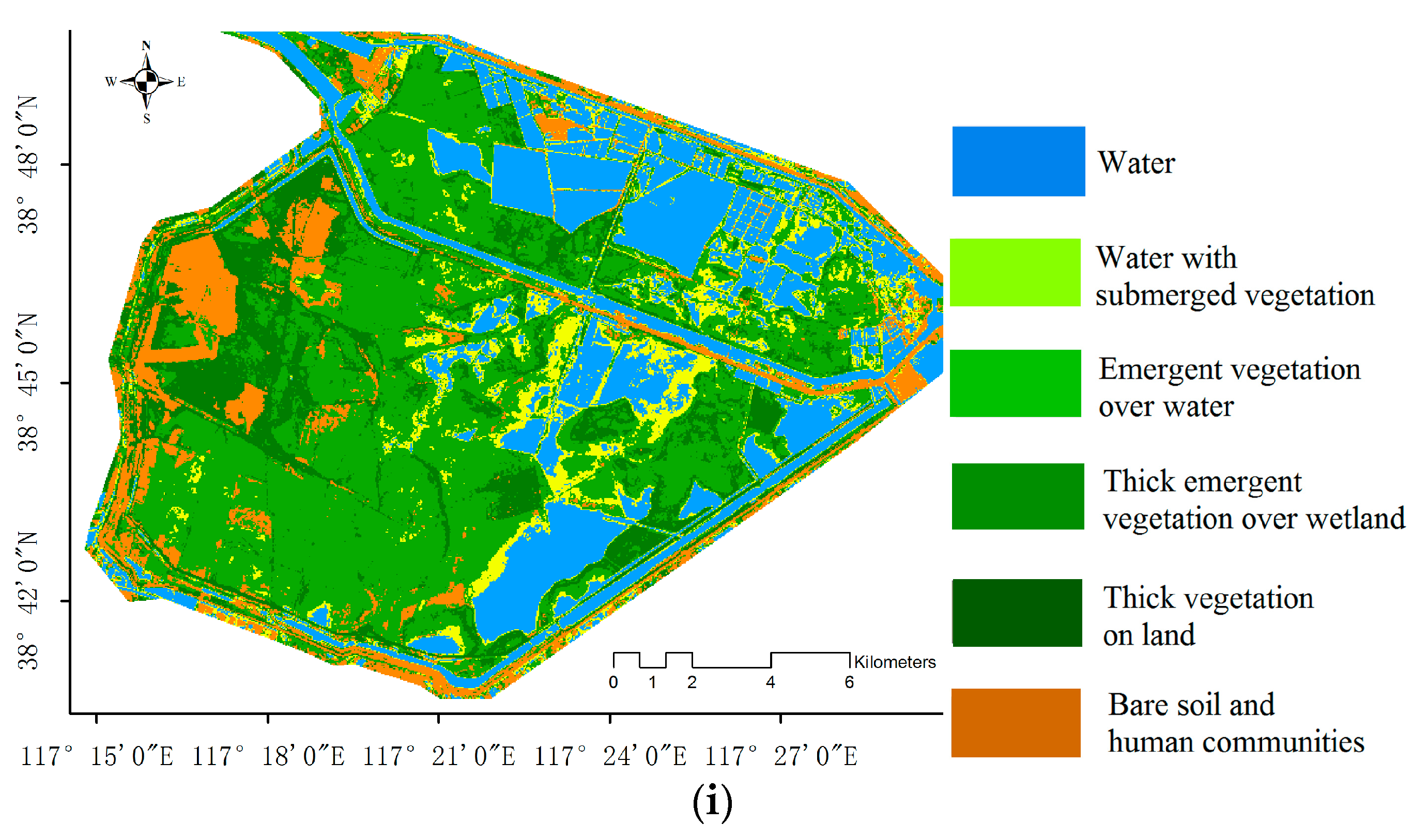
5.4. Forty-Year Spatial and Temporal Dynamics of the Beidagang Wetland Based on a Long-Term Series of Landsat Data
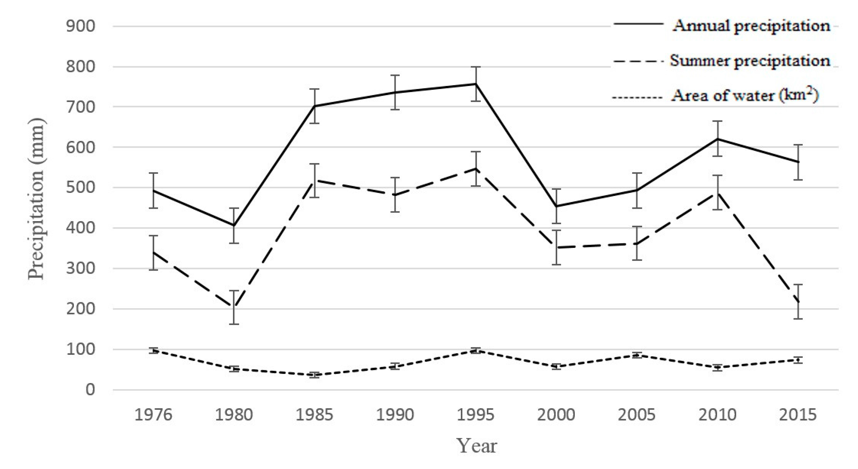
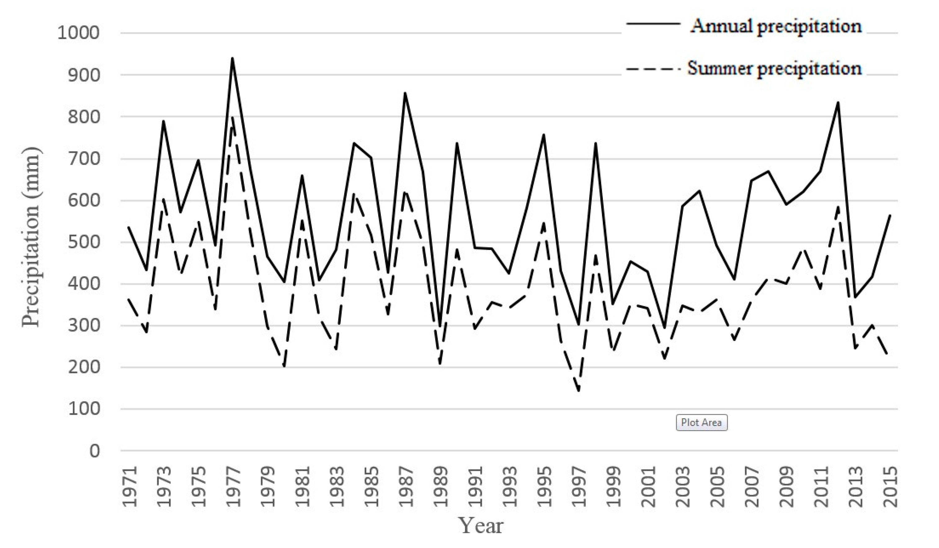
5.4.1. The Dynamics of Water and Analysis of the Associated Driving Factors
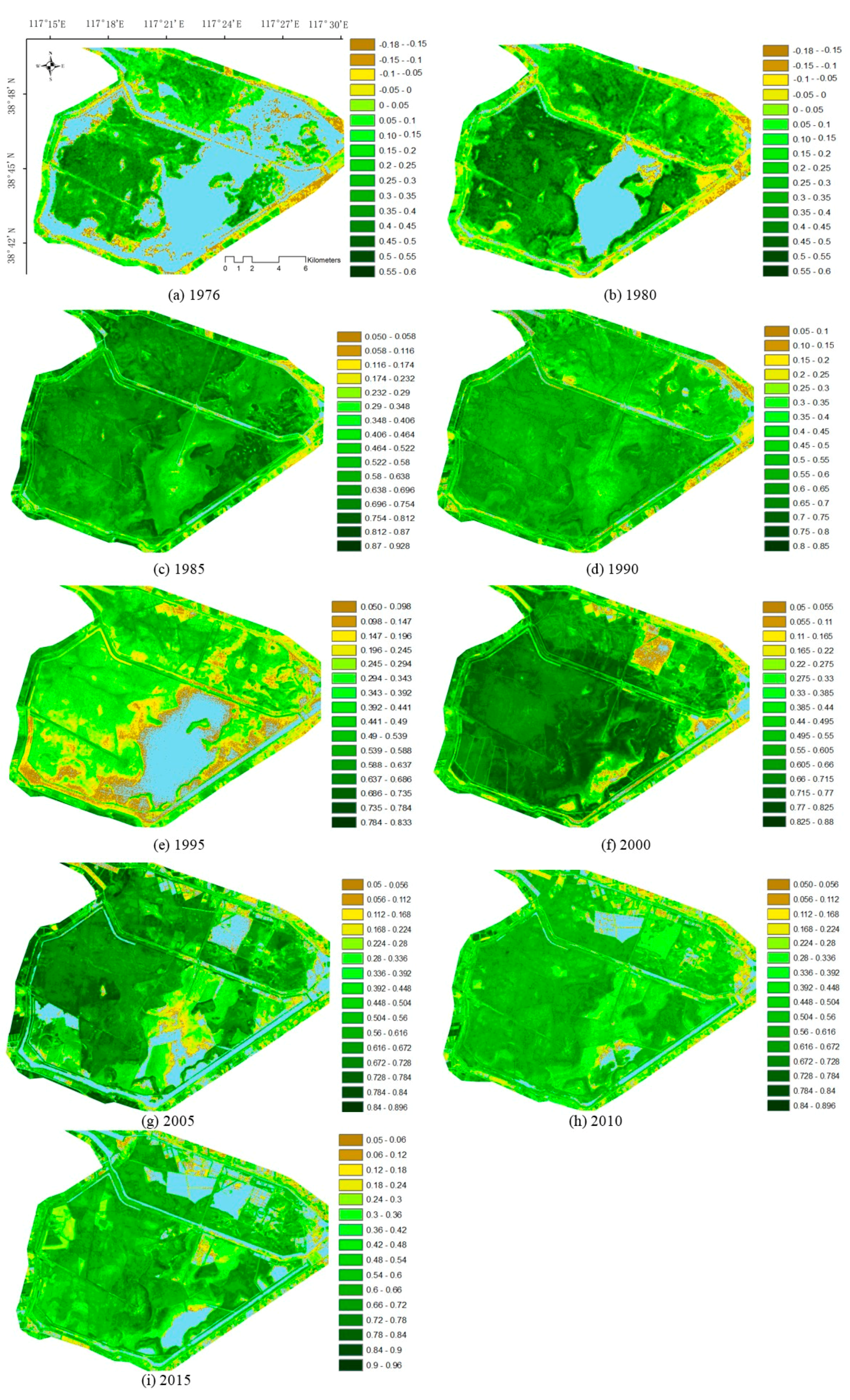
5.4.2. The Dynamics of the Vegetation Index
5.4.3. Changes in Vegetation Types Based on Water Resource Dynamics
6. Conclusions
Acknowledgments
Author Contributions
Conflicts of Interest
References
- Cowardin, L.M.; Carter, V.; Golet, F.C.; LaRoe, E.T. Classification of Wetlands and Deepwater Habitats of the United States; U.S. Department of the Interior Fish and Wildlife Services: Falls Church, VI, USA; 1979; Volume 79, p. 131.
- Semlitsch, R.D.; Bodie, J.R. Are small, isolated wetlands expendable? Conserv. Biol. 1998, 12, 1129–1133. [Google Scholar] [CrossRef]
- Ozesmi, S.L.; Bauer, M.E. Satellite remote sensing of wetlands. Wetl. Ecol. Manag. 2002, 10, 381–402. [Google Scholar] [CrossRef]
- Töyrä, J.; Pietroniro, A. Towards operational monitoring of a northern wetland using geomatics-based techniques. Remote Sens. Environ. 2005, 97, 174–191. [Google Scholar] [CrossRef]
- Kashaigili, J.J.; Mbilinyi, B.P.; Mccartney, M.; Mwanuzi, F.L. Dynamics of Usangu plains wetlands: Use of remote sensing and GIS as management decision tools. Phys. Chem. Earth Parts A/B/C 2006, 31, 967–975. [Google Scholar] [CrossRef]
- Odum, E.P. Ecology and Our Endangered Life-Support Systems; Sinauer Associates: Washington, DC, USA, 1989. [Google Scholar]
- Morris, J.T.; Sundareshwar, P.; Nietch, C.T.; Kjerfve, B.; Cahoon, D.R. Responses of coastal wetlands to rising sea level. Ecology 2002, 83, 2869–2877. [Google Scholar] [CrossRef]
- Leng, P.; Song, X.; Li, Z.-L.; Ma, J.; Zhou, F.; Li, S. Bare surface soil moisture retrieval from the synergistic use of optical and thermal infrared data. Int. J. Remote Sens. 2014, 35, 988–1003. [Google Scholar] [CrossRef]
- Gibbs, J.P. Importance of small wetlands for the persistence of local populations of wetland-associated animals. Wetlands 1993, 13, 25–31. [Google Scholar] [CrossRef]
- Babbitt, K.J. The relative importance of wetland size and hydroperiod for amphibians in southern New Hampshire, USA. Wetlands Ecol. Manag. 2005, 13, 269–279. [Google Scholar] [CrossRef]
- Klemas, V. Remote sensing of wetlands: case studies comparing practical techniques. J. Coast. Res. 2011, 27, 418–427. [Google Scholar] [CrossRef]
- Robertson, L.D.; King, D.J.; Davies, C. Assessing Land Cover Change and Anthropogenic Disturbance in Wetlands Using Vegetation Fractions Derived from Landsat 5 TM Imagery (1984–2010). Wetlands 2015, 35, 1077–1091. [Google Scholar] [CrossRef]
- Leng, P.; Song, X.; Duan, S.-B.; Li, Z.-L. A practical algorithm for estimating surface soil moisture using combined optical and thermal infrared data. Int. J. Appl. Earth Obs. Geoinf. 2016, 52, 338–348. [Google Scholar] [CrossRef]
- Bischof, H.; Schneider, W.; Pinz, A.J. Multispectral classification of Landsat-images using neural networks. IEEE Trans. Geosci. Electron. 1992, 30, 482–490. [Google Scholar] [CrossRef]
- Andres, L.; Salas, W.A.; Skole, D. Fourier analysis of multi-temporal AVHRR data applied to a land cover classification. Remote Sens. 1994, 15, 1115–1121. [Google Scholar] [CrossRef]
- Muchoney, D.; Borak, J.; Chi, H.; Friedl, M.; Gopal, S.; Hodges, J.; Morrow, N.; Strahler, A. Application of the MODIS global supervised classification model to vegetation and land cover mapping of Central America. Int. J. Remote Sens. 2000, 21, 1115–1138. [Google Scholar] [CrossRef]
- Zhu, Z.; Woodcock, C.E. Continuous change detection and classification of land cover using all available Landsat data. Remote Sens. Environ. 2014, 144, 152–171. [Google Scholar] [CrossRef]
- Liu, J.; Zhuang, D.; Luo, D.; Xiao, X.-M. Land-cover classification of China: Integrated analysis of AVHRR imagery and geophysical data. Int. J. Remote Sens. 2003, 24, 2485–2500. [Google Scholar] [CrossRef]
- Zhu, G.; Blumberg, D.G. Classification using ASTER data and SVM algorithms: The case study of Beer Sheva, Israel. Remote Sens. Environ. 2002, 80, 233–240. [Google Scholar] [CrossRef]
- Harada, I.; Hara, K.; Tomita, M.; Short, K.; Park, J. Monitoring landscape changes in Japan using classification of MODIS data combined with a landscape transformation sere (LTS) model. J. Landsc. Ecol. 2015, 7, 23–38. [Google Scholar] [CrossRef]
- Cannon, R.L.; Dave, J.V.; Bezdek, J.C.; Trivedi, M.M. Segmentation of a thematic mapper image using the fuzzy c-means clusterng algorthm. IEEE Trans. Geosci. Electron. 1986, 24, 400–408. [Google Scholar] [CrossRef]
- Robinson, V.; Strahler, A. Issues in designing geographic information systems under conditions of inexactness. In Proceedings of the 10th International Symposium on Machine Processing of Remotely Sensed Data: Thematic Mapper Data and Geographic Information Systems, Lafayette, IN, USA, 12–14 June 1984; pp. 198–204. [Google Scholar]
- Fisher, P.F. Remote sensing of land cover classes as type 2 fuzzy sets. Remote Sens. Environ. 2010, 114, 309–321. [Google Scholar] [CrossRef]
- Ngo, L.T.; Mai, D.S.; Pedrycz, W. Semi-supervising Interval Type-2 Fuzzy C-Means clustering with spatial information for multi-spectral satellite image classification and change detection. Comput. Geosci. 2015, 83, 1–16. [Google Scholar] [CrossRef]
- Bouchachia, A.; Pedrycz, W. Enhancement of fuzzy clustering by mechanisms of partial supervision. Fuzzy Sets Syst. 2006, 157, 1733–1759. [Google Scholar] [CrossRef]
- Shao, P.; Shi, W.; He, P.; Hao, M.; Zhang, X. Novel approach to unsupervised change detection based on a robust semi-supervised FCM clustering algorithm. Remote Sens. 2016, 8, 264. [Google Scholar] [CrossRef]
- Liu, H.; Zhao, F.; Jiao, L. Fuzzy spectral clustering with robust spatial information for image segmentation. Appl. Soft Comput. 2012, 12, 3636–3647. [Google Scholar] [CrossRef]
- Zhao, F.; Fan, J.; Liu, H. Optimal-selection-based suppressed fuzzy c-means clustering algorithm with self-tuning non local spatial information for image segmentation. Expert Syst. Appl. 2014, 41, 4083–4093. [Google Scholar] [CrossRef]
- Wang, Z.; Song, Q.; Soh, Y.C.; Sim, K. An adaptive spatial information-theoretic fuzzy clustering algorithm for image segmentation. Comput. Vis. Image Underst. 2013, 117, 1412–1420. [Google Scholar] [CrossRef]
- Nguyen, D.D.; Ngo, L.T.; Pham, L.T.; Pedrycz, W. Towards hybrid clustering approach to data classification: Multiple kernels based interval-valued Fuzzy C-Means algorithms. Fuzzy Sets Syst. 2015, 279, 17–39. [Google Scholar] [CrossRef]
- Zadeh, L.A. The concept of a linguistic variable and its application to approximate reasoning—I. Inf. Sci. 1975, 8, 199–249. [Google Scholar] [CrossRef]
- Mendel, J.M.; John, R.B. Type-2 fuzzy sets made simple. IEEE Trans. Fuzzy syst. 2002, 10, 117–127. [Google Scholar] [CrossRef]
- John, R.; Coupland, S. Type-2 fuzzy logic: A historical view. IEEE Comput. Intell. Mag. 2007, 2, 57–62. [Google Scholar] [CrossRef]
- Stavrakoudis, D.G.; Theocharis, J.B.; Zalidis, G.C. A boosted genetic fuzzy classifier for land cover classification of remote sensing imagery. ISPRS J. Photogramm. Remote Sens. 2011, 66, 529–544. [Google Scholar] [CrossRef]
- Ghaffarian, S. Automatic histogram-based fuzzy C-means clustering for remote sensing imagery. ISPRS J. Photogramm. Remote Sens. 2014, 97, 46–57. [Google Scholar] [CrossRef]
- Ghosh, A.; Mishra, N.S.; Ghosh, S. Fuzzy clustering algorithms for unsupervised change detection in remote sensing images. Inf. Sci. 2011, 181, 699–715. [Google Scholar] [CrossRef]
- Guo, J.; Huo, H.; Peng, G. Interval Type-II Fuzzy C-Means Clustering based on Interval Number Distance and Ranking. IEEE Trans. Fuzzy Syst. 2017. under review. [Google Scholar]
- Guo, J.; Li, M.; Liu, D. Effects of urbanization on air temperature of Tianjin in recent 40 years. Ecol. Environ. Sci. 2009, 1, 29–34. [Google Scholar]
- Chen, Q.; Liu, D.; Ma, C. Productivity and N and P Nutrition of the Phragmites australis Community in Typical Wetlands in Tianjin and Their Relationships with Environmental Factors. J. Ecol. Rural Environ. 2016, 32, 60–67. [Google Scholar]
- National Science & Technology Infrastructure/China Meteorological Data Service Center (CMDC). Hourly Data from Surface Meteorological Stations in China. Available online: http://www.cma.gov.cn/2011qxfw/2011qsjgx/ (accessed on 22 August 2015).
- Ungar, S.G.; Pearlman, J.S.; Mendenhall, J.A.; Reuter, D. Overview of the earth observing one (EO-1) mission. IEEE Trans. Geosci. Electron. 2003, 41, 1149–1159. [Google Scholar] [CrossRef]
- Biggar, S.F.; Thome, K.J.; Wisniewski, W. Vicarious radiometric calibration of EO-1 sensors by reference to high-reflectance ground targets. IEEE Trans. Geosci. Electron. 2003, 41, 1174–1179. [Google Scholar] [CrossRef]
- Drusch, M.; Del Bello, U.; Carlier, S.; Colin, O.; Fernandez, V.; Gascon, F.; Hoersch, B.; Isola, C.; Laberinti, P.; Martimort, P.; et al. Sentinel-2: ESA’s optical high-resolution mission for GMES operational services. Remote Sens. Environ. 2012, 120, 25–36. [Google Scholar] [CrossRef]
- Sentinel Application Platform (SNAP)/European Space Agency (ESA). Science Toolbox Exploitation Platform. Available online: http://step.esa.int/main/toolboxes/snap/ (accessed on 23 June 2015).
- Copernicus Space Component—Ground Segment team/ European Space Agency (ESA). Sentinels Data Products List. Available online: https://earth.esa.int/web/sentinel/missions/sentinel-2/data-products (accessed on 23 June 2015).
- Chander, G.; Markham, B.L.; Helder, D.L. Summary of current radiometric calibration coefficients for Landsat MSS, TM, ETM+, and EO-1 ALI sensors. Remote Sens. Environ. 2009, 113, 893–903. [Google Scholar] [CrossRef]
- EarthExplorer/United States Geological Survey. Bulk Download of Satellite Imagery Using EarthExplorer. Available online: https://earthexplorer.usgs.gov (accessed on 29 May 2016).
- Feng, M.; Sexton, J.O.; Huang, C.; Masek, J.G.; Vermote, E.F.; Gao, F.; Narasimhan, R.; Channan, S.; Wolfe, R.E.; Townshend, J.R. Global surface reflectance products from Landsat: Assessment using coincident MODIS observations. Remote Sens. Environ. 2013, 134, 276–293. [Google Scholar] [CrossRef]
- Vermote, E.; Saleous, N. LEDAPS Surface Reflectance Product Description; University of Maryland: College Park, MD, USA, 2007. [Google Scholar]
- Vuolo, F.; Mattiuzzi, M.; Atzberger, C. Comparison of the Landsat Surface Reflectance Climate Data Record (CDR) and manually atmospherically corrected data in a semi-arid European study area. Int. J. Appl. Earth Obs. Geoinf. 2015, 42, 1–10. [Google Scholar] [CrossRef]
- Bezdek, J.C. Pattern Recognition with Fuzzy Objective Function Algorithms; Plenum Press: New York, NY, USA, 1981. [Google Scholar]
- Hwang, C.; Rhee, F.C.H. Uncertain fuzzy clustering: Interval Type-2 fuzzy approach to C-means. IEEE Trans. Fuzzy Syst. 2007, 15, 107–120. [Google Scholar] [CrossRef]
- Karnik, N.N.; Mendel, J.M. Centroid of a type-2 fuzzy set. Inf. Sci. 2001, 132, 195–220. [Google Scholar] [CrossRef]
- Zarinbal, M.; Zarandi, M.F.; Turksen, I.B. Interval Type-2 Relative Entropy Fuzzy C-Means clustering. Inf. Sci. 2014, 272, 49–72. [Google Scholar] [CrossRef]
- Min, J.; Shim, E.A.; Rhee, F.C.H. An interval type-2 fuzzy PCM algorithm for pattern recognition. In Proceedings of the 18th International Conference on Fuzzy Systems (Fuzz-IEEE ’09), Jeju Island, South Korea, 20–24 August 2009; pp. 480–483. [Google Scholar]
- Ji, Z.; Xia, Y.; Sun, Q.; Cao, G. Interval-valued possibilistic fuzzy C-means clustering algorithm. Fuzzy Sets Syst. 2014, 253, 138–156. [Google Scholar] [CrossRef]
- Ondrej, L.; Milos, M. General Type-2 fuzzy C-Means algorithm for uncertain fuzzy clustering. IEEE Trans. Fuzzy Syst. 2012, 20, 883–897. [Google Scholar]
- Swain, P.H.; Davis, S.M. Remote Sensing: The Quantitative Approach; McGraw-Hill: New York, NY, USA, 1978. [Google Scholar]
- Cheng, J.; Guo, H.; Shi, W. Uncertainty of Remote Sensing Data; Chinese Science Press: Beijing, China, 2004. [Google Scholar]
- Shi, W. Principles of Modeling Uncertainties in Spatial Data and Spatial Analyses; CRC Press: Boca Raton, FL, USA, 2009. [Google Scholar]
- Huang, J.; Wang, X.; Wang, F. Uncertainty in Padday Rice Remote Sensing; Zhejiang University Press: Hangzhou, China, 2013. [Google Scholar]
- Wang, Q.; Shi, W. Unsupervised classification based on fuzzy c-means with uncertainty analysis. Remote Sens. Lett. 2013, 4, 1087–1096. [Google Scholar] [CrossRef]
- Yu, X.; He, H.; Hu, D.; Zhou, W. Land cover classification of remote sensing imagery based on interval-valued data fuzzy c-means algorithm. Sci. China Earth Sci. 2014, 57, 1306–1313. [Google Scholar] [CrossRef]
- Li, X.; Zhang, S. Rank of interval numbers based on a new distance measure. J. Xihua Univ. (Nat. Sci.) 2008, 27, 87–90. [Google Scholar]
- Xiao, J.; Zhang, Y.; Fu, C. Comparison between Methods of Interval Number Ranking Based on Possibility. J. Tianjin Univ. 2011, 44, 705–711. [Google Scholar]
- Wang, W.; Zhang, Y. On fuzzy cluster validity indices. Fuzzy Sets Syst. 2007, 158, 2095–2117. [Google Scholar] [CrossRef]
- Fukuyama, Y.; Sugeno, M. A new method of choosing the number of clusters for the fuzzy C-means method. In Proceedings of the Fifth Fuzzy Systems Symposium, Kobe, Japan, 2–3 June 1989; pp. 247–250. [Google Scholar]
- Xie, X.L.; Beni, G. A validity measure for fuzzy clustering. IEEE Trans. Pattern Anal. Mach. Intell. 1991, 13, 841–847. [Google Scholar] [CrossRef]
- Li, H.; Zhang, S.; Ding, X.; Zhang, C.; Dale, P. Performance evaluation of cluster validity indices (CVIs) on Multi/Hyperspectral remote sensing datasets. Remote Sens. 2016, 8, 295. [Google Scholar] [CrossRef]
- Yuan, F.; Bauer, M.E. Comparison of impervious surface area and normalized difference vegetation index as indicators of surface urban heat island effects in Landsat imagery. Remote Sens. Environ. 2007, 106, 375–386. [Google Scholar] [CrossRef]
- Bezdek, J.C.; Ehrlich, R.; Full, W. FCM: The fuzzy c-means clustering algorithm. Comput. Geosci. 1984, 10, 191–203. [Google Scholar] [CrossRef]
- Zlinszky, A.; Kania, A. Will it blend? Visualization and accuracy evaluation of high-resolution fuzzy vegetation maps. Int. Arch. Photogramm. Remote Sens. Spat. Inf. Sci. 2016, XLI-B2, 335–343. [Google Scholar] [CrossRef]


| Year | Landsat Date | Sensor | Cloud Cover (%) |
|---|---|---|---|
| 1976 | 09/19 | Landsat 2/MSS | 0.00 |
| 1980 | 09/17 | Landsat 2/MSS | 0.00 |
| 1985 | 08/28 | Landsat 5/TM | 5.93 |
| 1990 | 09/11 | Landsat 5/TM | 1.46 |
| 1995 | 08/24 | Landsat 5/TM | 1.15 |
| 2000 | 08/21 | Landsat 5/TM | 6.39 |
| 2005 | 09/04 | Landsat 5/TM | 7.50 |
| 2010 | 10/04 | Landsat 5/TM | 0.16 |
| 2015 | 10/02 | Landsat 8/OLI | 0.33 |
| 2016 | 05/29 | Landsat 8/OLI | 7.43 |
| Dataset | Validity Index | IT2FCM | IT2FCM* |
|---|---|---|---|
| EO-1 ALI 22 August 2015 | PC- | 0.27 | 0.36 |
| PE- | 1.33 | 1.28 | |
| FS- | −1449.52 | −2199.84 | |
| XB- | 0.40 | 0.37 | |
| Landsat 8/OLS 29 May 2016 | PC- | 0.22 | 0.29 |
| PE- | 1.54 | 1.49 | |
| FS- | −6.041347175E7 | −1.1131032418E8 | |
| XB- | 0.52 | 0.35 | |
| Sentine-2 30 May 2016 | PC- | 0.21 | 0.26 |
| PE- | 1.59 | 1.47 | |
| FS- | −3.725715410E7 | −7.483440017E7 | |
| XB- | 0.30 | 0.27 |
© 2017 by the authors. Licensee MDPI, Basel, Switzerland. This article is an open access article distributed under the terms and conditions of the Creative Commons Attribution (CC BY) license (http://creativecommons.org/licenses/by/4.0/).
Share and Cite
Huo, H.; Guo, J.; Li, Z.-L.; Jiang, X. Remote Sensing of Spatiotemporal Changes in Wetland Geomorphology Based on Type 2 Fuzzy Sets: A Case Study of Beidagang Wetland from 1975 to 2015. Remote Sens. 2017, 9, 683. https://doi.org/10.3390/rs9070683
Huo H, Guo J, Li Z-L, Jiang X. Remote Sensing of Spatiotemporal Changes in Wetland Geomorphology Based on Type 2 Fuzzy Sets: A Case Study of Beidagang Wetland from 1975 to 2015. Remote Sensing. 2017; 9(7):683. https://doi.org/10.3390/rs9070683
Chicago/Turabian StyleHuo, Hongyuan, Jifa Guo, Zhao-Liang Li, and Xiaoguang Jiang. 2017. "Remote Sensing of Spatiotemporal Changes in Wetland Geomorphology Based on Type 2 Fuzzy Sets: A Case Study of Beidagang Wetland from 1975 to 2015" Remote Sensing 9, no. 7: 683. https://doi.org/10.3390/rs9070683