
Optimal Seamline Detection for Orthoimage Mosaicking by Combining Deep Convolutional Neural Network and Graph Cuts


1
School of Remote Sensing and Information Engineering, Wuhan University, Wuhan 430079, Hubei, China
2
Center for Spatial Information Science, University of Tokyo, Kashiwa 277-8568, Japan
3
China Transport Telecommunications and Information Center, Beijing 100011, China
*
Author to whom correspondence should be addressed.
Remote Sens. 2017, 9(7), 701; https://doi.org/10.3390/rs9070701
Submission received: 21 April 2017
/
Revised: 13 June 2017
/
Accepted: 5 July 2017
/
Published: 7 July 2017
Abstract
:When mosaicking orthoimages, especially in urban areas with various obvious ground objects like buildings, roads, cars or trees, the detection of optimal seamlines is one of the key technologies for creating seamless and pleasant image mosaics. In this paper, we propose a new approach to detect optimal seamlines for orthoimage mosaicking with the use of deep convolutional neural network (CNN) and graph cuts. Deep CNNs have been widely used in many fields of computer vision and photogrammetry in recent years, and graph cuts is one of the most widely used energy optimization frameworks. We first propose a deep CNN for land cover semantic segmentation in overlap regions between two adjacent images. Then, the energy cost of each pixel in the overlap regions is defined based on the classification probabilities of belonging to each of the specified classes. To find the optimal seamlines globally, we fuse the CNN-classified energy costs of all pixels into the graph cuts energy minimization framework. The main advantage of our proposed method is that the pixel similarity energy costs between two images are defined using the classification results of the CNN based semantic segmentation instead of using the image informations of color, gradient or texture as traditional methods do. Another advantage of our proposed method is that the semantic informations are fully used to guide the process of optimal seamline detection, which is more reasonable than only using the hand designed features defined to represent the image differences. Finally, the experimental results on several groups of challenging orthoimages show that the proposed method is capable of finding high-quality seamlines among urban and non-urban orthoimages, and outperforms the state-of-the-art algorithms and the commercial software based on the visual comparison, statistical evaluation and quantitative evaluation based on the structural similarity (SSIM) index.
1. Introduction
Digital orthophoto map (DOM) is one of the most popularly used products in the field of photogrammetry, and it can provide both pleasant textures and accurate geometric properties of maps. However, to produce a large-scale orthophoto, we need to stitch a large set of orthoimages into the single composite image due to fact that the covered region of a single orthoimage is limited. Therefore, image mosaicking is one of the key technologies to generate a large-scale DOM. It also is an important and classical problem in the fields of photogrammetry [1,2,3,4,5], remote sensing [6,7] and computer vision [8,9,10], which is used to merge a set of geometrically aligned images into a single composite image as seamlessly as possible. In an ideally static scene in which both the photometric inconsistencies and the geometric misalignments are not existing or not obviously visible in overlap regions, the mosaicked image always looks perfect only when the geometric distance criterion is used. However, in some cases, there exist photometric inconsistencies to different extents in overlap regions between images due to illumination variations and different exposure settings. This problem can be solved well by a series of color correction and image blending approaches [11,12]. In addition, in orthoimages, the geometric positions of corresponding pixels on obvious ground objects from different images may be different if they are not included in the digital terrain model (DTM) or wrongly modeled [6]. Therefore, the visible seams in those object regions may appear if the seamlines cross them. The effective way to solve this problem is to detect the optimal seamlines to avoid crossing majority of visually obvious objects and most of the overlap regions with low image similarity and large object dislocation. In this paper, our work focuses on detecting the optimal seamlines between overlapped images to eliminate the influences of geometric misalignments.
Optimal seamline detection methods search for the seamlines in overlap regions between adjacent images where their intensity or gradient differences are minimal, especially avoiding crossing the obvious ground objects like buildings and cars. Most of the optimal seamline detection methods formulated it as an energy minimization problem. Generally, those methods can be implemented in two stages. In the first stage, the cost images are defined to represent the differences between the original images. In the second stage, the optimal seamlines are further found based on the cost images via different optimization algorithms, e.g., snake model [13], Dijkstra’s algorithm [14], dynamic programming [15], and graph cuts [16]. The major issues of optimal seamline detection focus on how to define the cost images more reasonably and how to find the seamlines more efficiently and effectively. According to the used optimization algorithms, we simply review recently proposed seamline detection approaches in the following.
Kerschner [6] proposed an automated seamline detection method using twin snake based on the energy function defined on the similarity of color and texture. The energy optimization started from two snakes on the opposite borders of the overlap region, which moved closer during the energy minimization process, and the optimal seamline was found when two twin snakes coincided. However, this algorithm requires a high computation cost and cannot overcome the local minimum problem. Wang et al. [17] proposed an improved snake model to detect the seamline. In this algorithm, the sum of the mismatched values on the seamline was defined as the energy function, and then the seamline with the lowest energy was regarded as the final optimal seamline. This improved snake model solves the local optimum problem existed in the snake model to some extent, but not completely.
Besides the snake model, the Dijkstra’s algorithm is also popularly used for detecting the optimal seamlines. Chon et al. [1] designed a novel objective function to evaluate the mismatching between two images based on the normalized cross correlation (NCC). Their proposed method first determined the desired level of maximum difference along the seamline and then applied the Dijkstra’s algorithm to find the best seamline with the minimal objective function. Compared with the simple Dijkstra’s algorithm, their method could find a longer seamline with less pixels with high energy costs. Pan et al. [4] proposed a new method for seamline detection based on segmentation. It first determined the preferred regions based on the spans of segments generated by the meanshift algorithm. Then, the last pixel-level seamline was detected by using the Dijkstra’s algorithm on the cost image defined by intensity differences. After that, several object-based algorithms [18,19] were proposed to detect high-quality seamlines. In addition, Chen et al. [20] proposed a new automatic seamline selection algorithm by using the digital surface model (DSM). It found the optimal seamline via the Dijkstra’s algorithm under the guide of the elevation information extracted from DSM. Similarly, Pang et al. [21] guided the seamline with the corresponding pixel-wise disparity generated by a semi-global matching (SGM) algorithm. Similar with the Dijkstra’s algorithm, the Floyd–Warshall shortest path algorithm [22] can also be used to find the optimal seamline. Wan et al. [3] proposed a vector road-based seamline determination algorithm ensuring that the seamline follows the centerlines of wide streets and avoids crossing foreground objects. This algorithm firstly built a weighted graph by overlapping the extracted skeleton of the overlap regions and vector roads, and then found the lowest cost path between two intersections of adjacent image polygons by applying the Floyd–Warshall algorithm.
The dynamic-programming-based optimal seamline detection strategy can also be used for optimal seamline detection, which is less time-consuming than the Dijkstra’s algorithm. Yu et al. [2] proposed to combine the pixel-based similarity defined by color, edge and texture informations with the region-based saliency map based on the human attention model to guide the optimal seamline searching process of the dynamic programming (DP) algorithm. Zeng et al. [23] proposed a new optimal searching criterion that combines the gradient difference and the edge-enhanced weighting intensity one, which provides an effective mechanism for avoiding problems caused by moving objects and geometric misalignments. Then, this algorithm applied dynamic programming to find the optimal seamline.
In addition, graph cuts has also been popularly applied to find the optimal seamlines. Graph cuts [16] is an efficient energy optimization algorithm to solve labeling problems and has been widely utilized in many applications of image processing and computer vision, such as image segmentation, stereo matching, and image blending [5,9,10,24]. The basic idea of graph cuts is to first construct a weighted graph where each edge weight cost represents the corresponding cost energy value, and then to find the minimum cut in this graph based on the max-flow or min-cut algorithm [25]. To some extent, the optimal seamline detection problem can be regarded as the inverse process of image segmentation. The aim of image segmentation is to separate the segments in the positions with large differences between adjacent pixels. In contrast, the optimal seamline locates on the positions with small differences between adjacent images. Therefore, the optimal seamline can be detected via graph cuts as image segmentation does. Kwatra et al. [24] first applied the graph cuts algorithm to find the seamline for image and video synthesis. Their proposed method defined an energy function based on the difference of color intensities and gradient magnitudes along horizontal and vertical directions and then applied graph cuts to find optimal seamlines. Agarwala et al. [10] provided a framework to easily create a single composite image using graph cuts to choose good seamlines within the constituent images, which needs an intuitive human–computer interaction for defining local and global objectives. Gracias et al. [9] combined the watershed segmentation and the graph cuts algorithm to detect the optimal seamlines. Their algorithm began with creating a set of watershed segments on the difference image of overlap regions followed by finding the solution via graph cuts between those segments instead of the entire set of pixels. Li et al. [5] first defined the cost image by combining the informations of image color, gradient and texture complexity, and then found the optimal seamline via graph cuts.
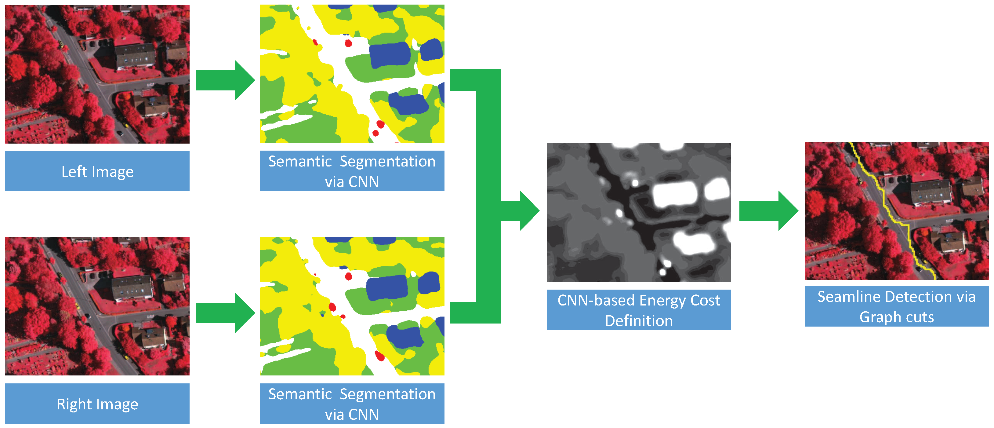
By the review of the above-mentioned optimal seamline detection methods, we can find that many features (intensity, color, gradient, texture, road vector, saliency, segments, disparity and DSM, and so on) have been used to guide the optimal seamline searching process. However, those features cannot completely describe the differences between overlapped images independently, and it is also difficult to find the best combination of several features to represent the differences. Therefore, in this paper, we propose a new optimal seamline detection method based on the scene semantic segmentation using convolutional neural network (CNN). The energy costs are defined based on the classification results of CNN, instead of combining many different hand-designed features. The workflow of our method is presented in Figure 1. Firstly, we manually label the remote sensing image data into several most cover classes as the training data, which is then used to train our proposed fully convolutional network for semantic segmentation. Secondly, the overlap regions of the left and right images are classified via the trained network independently, and we can obtain the probabilities of each pixel belonging to each of the specified classes. Finally, we define the energy costs based on those classification probabilities, and find the optimal seamlines via graph cuts. In addition, the detected seamlines are evaluated quantitatively based on the defined quality measurements. The main contributions of our proposed approach are summarized as follows:
- We design a novel energy function to guide the searching process of optimal seamlines between two input geometrical aligned images. This energy function is defined by using the semantic segmentation results generated by CNN. Thus, we do not need to design the features for optimal seamline detection anymore. The experiments proved that this energy function performs well in avoiding crossing obvious objects because it can distinguish the whole regions of obvious objects from the images.
- We fuse the defined energy function into the graph cuts optimization framework to find the optimal seamlines with minimum energy cost, and we propose using the structural similarity (SSIM) index to quantitatively evaluate the qualities of detected seamlines. We test our proposed approach in several groups of images captured from different places and prove that our proposed approach outperforms the state-of-the-art approaches and commercial software.
The remaining part of this paper is organized as follows. Section 2 introduces the training data and the convolutional neural network for semantic image segmentation used in our paper. Section 3 introduces the graph cuts energy minimization framework for finding the optimal seamline between two images based on the CNN-based energy costs, and the method for quality assessment of mosaicked images is presented in Section 4. Experimental results on several groups of challenging orthoimages are presented in Section 5 followed by the conclusions drawn in Section 6.
2. Semantic Image Segmentation
In our proposed seamline detection method, the energy cost of each pixel is defined based on its classification results with the deep CNN for semantic image segmentation. In this section, we will give detailed description about the semantic image segmentation network used in this paper. We first describe the used pixel-to-pixel architecture, which allows us to obtain dense semantic segmentation. Then, we will illustrate the network training process and related strategies, including data preparation, model parameters, class balancing and loss function.
2.1. Model Architecture
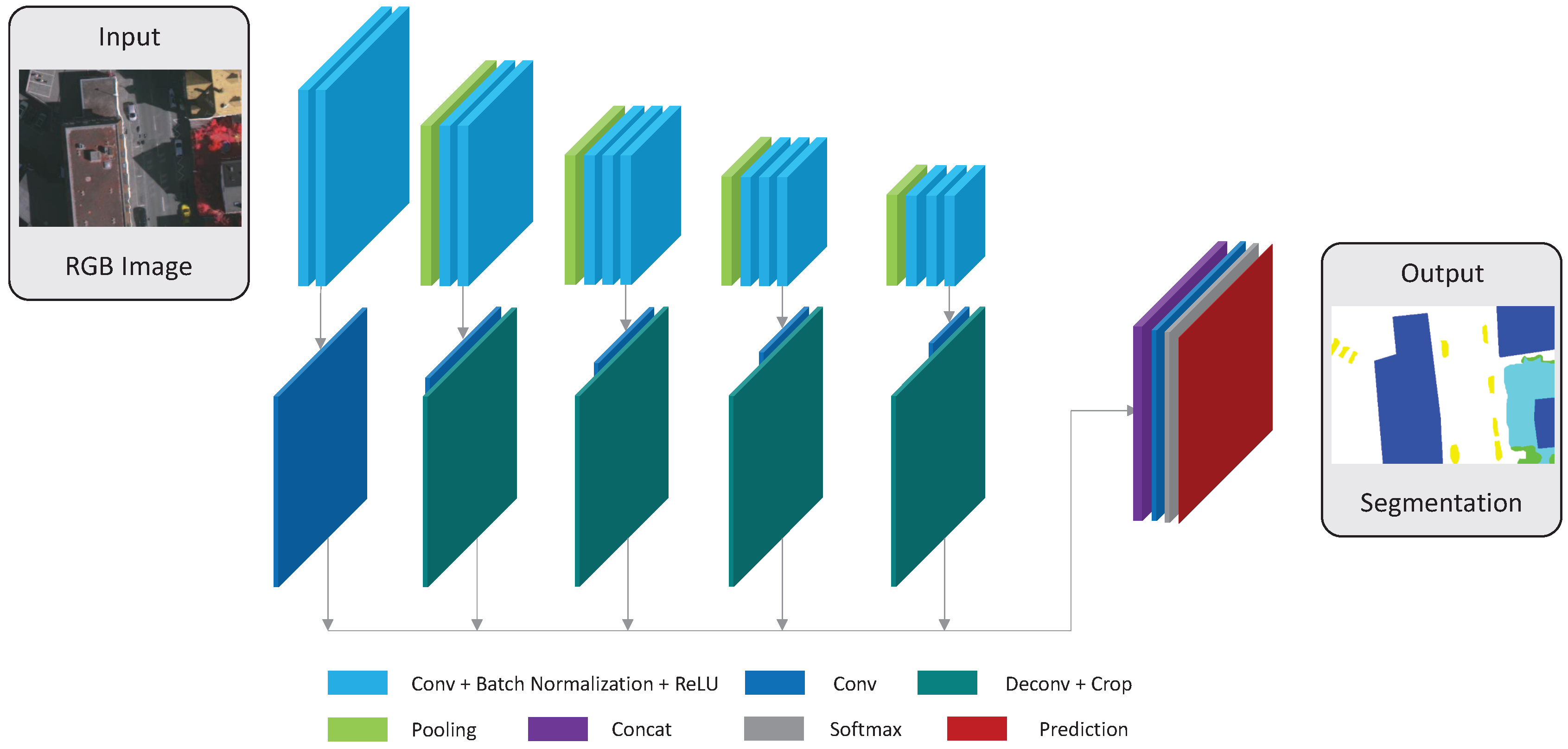
Inspired by the Fully Convolutional networks (FCN) architecture [26], we also design an architecture that allows the end-to-end learning of the pixel-to-pixel semantic segmentation. Therefore, for each pixel, we can obtain the probabilities of belonging to each of the special classes, which are used to define the energy costs for seamline detection. Our architecture fuses hierarchical features acquired from multiple layers to predict the last segmentation, as shown in Figure 2. We use the 13 convolutional layers that correspond to the first 13 convolutional layers in the VGG-16 net [27], which is designed for object classification. Each convolutional layer consists of convolution, batch normalization [28] and Rectified Linear Unit (ReLU) [29], and each set separated by the max-pooling layer. The max-pooling is performed over a 2 × 2 pixel window with a stride of two pixels (non-overlapping window). The side-output layer is generated by performing over a convolutional layer with a kernel size of 1 and a number of output K (the number of classes, used in our application). Except the first side-output layer, other side-output layers are followed by deconvolutional layers, which are applied to upsample the plane size of the feature maps back to the original image size. Here, all upsamplings are fixed to bilinear interpolation. Then, all side-output feature maps are concatenated into one feature map by using a concat layer, followed by a convolutional layer to reduce the dimension of the feature map and the softmax layer to predict the results of segmentation. In this way, the training network can learn multi-scale and multi-level features. This can improve the robustness of our training network. The output of the softmax layer is a K-channel probability map. Each channel of this map represents the probability of belongings to the corresponding class.
2.2. Data Preparation
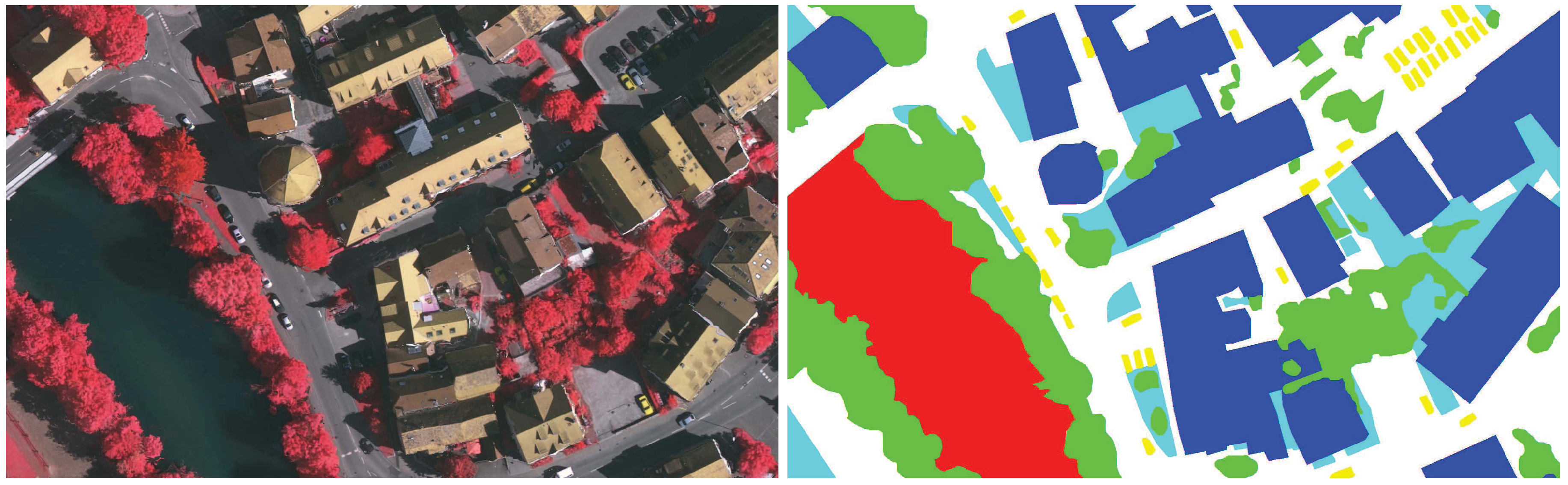
The training data is constructed by a set of aerial images and the corresponding manually-classified ground truth maps with multiple object classes such as building, car, tree, water, etc. A typical training sample is shown in Figure 3. Due to the limitation of GPU memory, the network will be trained in mini-batches on patches of , and the image patches are extracted from the input images with overlap and are flipped (left to right and up to down). No other data augmentation strategies are applied to increase the number of training data.
2.3. Model Parameters
The semantic segmentation network is trained by using the publicly available Caffe [30] library. We use the Stochastic Gradient Descent (SGD) [31] method to optimize our model. The model parameters used in this paper are listed as follows: the size of the input image (544 × 384 × 3), the size of the ground truth (544 × 384 × 1), the learning rate (1e-4), the reduce learning rate (reduces by 20 percent every 5e4 iterations), the training iterations (4e5), the mini-batch (1), the loss weight for each side-output layer and the final fused layer (1.0), the momentum (0.9), and the weight decay (2e-4). If not specifically stated in this paper, all experiments are conducted with this default settings.
2.4. Loss Function
As shown in Figure 4, each side-output layer is followed with a softmax layer in the process of network training. Each side-output layer can generate a prediction map for semantic segmentation, the corresponding loss function is denoted as . All side-output layers are concatenated into one layer to predict the last results of segmentation with the use of a softmax layer, and the loss function used in this softmax layer is denoted as , and the last overall loss function is defined as the sum of all side-output terms and fused loss term:
where denotes the loss weight for j-th side-output term, and represents the loss weight for fused loss term. In our model, all of those loss weights are set as as described in Section 2.3, and we use the cross-entropy classification loss [26,32] function to train our network. All loss functions and are defined by using the cross-entropy classification loss. In this way, this loss function is defined as:
where N is the number of pixels in a mini-batch, and denotes the probability of pixel belonging to the ground truth class c.
2.5. Class Balancing
As presented in Section 2.4, we use the cross-entropy loss function to train our FCN-based semantic segmentation network. However, because this loss is calculated by summing over all pixels, it does not account well for imbalanced classes. For the classes with relatively less covered regions, such as cars, according to the traditional cross-entropy loss function, those classes contribute little to the last overall loss function. Therefore, to take the imbalanced classes into account, we need to weight the losses to balance the influences among all classes, namely, class balancing [32]. We use the median frequency balancing [33] to weight each class in the loss function. The median frequency balancing weights the loss of classes by using the ratio of the median class frequency in the training dataset and the actual class frequency. The cross-entropy classification loss is modified as:
where is the corresponding weight defined as:
where denotes the frequency of pixels in the class c, and denotes the set of all classes.
3. CNN-Based Seamline Detection via Graph Cuts
In this paper, we formulate the optimal seamline detection as an energy minimization optimization problem based on the semantic image segmentation results, and solve it by using the graph cuts algorithm as Li et al. [5] do. We first briefly review the optimal seamline detection algorithm proposed by Li et al. [5]. Then, we will discuss the differences between it and our proposed algorithm, and present the motivation of our proposed method. Next, we also give more detailed description of our proposed CNN-based algorithm.
3.1. Brief Review on Li et al. algorithm
Here, we will briefly review the optimal seamline detection algorithm proposed by [5]. Their algorithm can be divided into two stages, namely, energy computation and labeling optimization. In the first stage, to effectively ensure that the seamlines are optimally detected in the laterally continuous regions with high image similarity and low object dislocation, Li et al. fused the information of image color, gradient magnitude and texture complexity to define the energy cost for each pixel. Especially, they proposed a new texture complexity measurement to distinguish the regions with smooth texture, such as roads, sky and woodlands. This measurement can be used to constrain the color differences and gradient magnitudes in the regions with smooth texture or repetitive patterns without affecting other foreground objects regions with rich and strong edges. In this way, the energy cost of each pixel in the overlap region can be computed. An example of last normalized energy cost map is shown in Figure 5c. In the second stage, they formulated the optimal seamline detection as a unified graph cuts energy minimization problem, as shown in Figure 6. They regarded each pixel as a node in the graph and assumed that each node has four cardinal neighbors. In this graph, it has two kinds of links. The first consists of the links between input images and the nodes, namely, t-link. Another is comprised of the links between two adjacent nodes, namely, n-link. Each link has corresponding weight cost. The costs of t-links and n-links are often called as the data energy term and the smooth energy term. For each node, its data energy cost only depends on whether this node is inside the valid region of one input image. For each pair of nodes, its smooth energy cost is defined as the sum of energy costs of these two nodes. After all energy functions have been defined as those used in the standard graph cuts energy minimization framework, they directly applied the graph cuts algorithm to find the optimal solution of the seamline in the overlap region between two geometrically aligned images.
3.2. CNN-Based Energy Cost Definition
The major difference between our proposed algorithm and the Li et al. algorithm [5] is the computation of energy cost, namely, the first stage. As shown in Figure 5, we present two normalized energy cost maps generated by our proposed CNN-based method and the Li et al. algorithm [5]. From Figure 5a,b, we observed that there are many obvious objects (buildings and cars), which are unsuitable to be passed through by the seamlines. However, we found that the roofs of those buildings have smooth textures, and small intensity and gradient differences, just like neighboring roads. The energy costs of those regions calculated by Li et al. [5] are small too, besides the regions of edges, as shown in Figure 5c. To solve this problem, we propose to define the energy cost based on the classification results of semantic image segmentation, as shown in Figure 5d, from which we observed that our defined energy cost map is more reasonable.
As we know, to avoid the appearance of artifacts along the seamlines, the detected optimal seamlines should be located on the regions with high similarity and low object dislocation, such as roads and grass, and avoid crossing the obvious objects, such as cars and buildings. Therefore, for different object classes, their penalty coefficients are different. For example, the penalty coefficients of buildings and cars should be larger than those of roads and grass. We denote all penalty coefficients as , where denotes the penalty coefficient of k-th object class and K is the number of the total object classes. For a pixel in one input image , or q, we can obtain the prediction probabilities of belonging to each class based on the semantic image segmentation results. The probabilities are represented as where denotes the probability of belonging to the k-th object class. Based on these probabilities, we can define the energy cost in one image as follows:
In addition, the final energy cost of is defined as the maximal value among two images as:
where A is a small constant to ensure that the energy cost is larger than 0.
In this paper, the test images are classified into six land cover classes, as shown in Figure 3. We order those classes as: (1) building; (2) car; (3) tree; (4) low vegetation; (5) water; (6) impervious surface. Of course, the penalty coefficients of low vegetation, water and impervious surface should be set as 0 because those regions are suitable to be passed through by seamlines. In addition, the penalty coefficients of buildings and cars should be set as the biggest value among all classes. The regions of trees are special. On the one hand, the texture of those tree regions is strongly repetitive, so the seams won’t be obviously visible if the seamlines cross them. On the other hand, the geometric positions of corresponding pixels on those tree regions from different images are different, and there exist geometric misalignments on those regions. Thus, we set the penalty coefficient of trees larger than 0 but smaller than the penalty coefficients of buildings and cars. In conclusion, we empirically set all penalty coefficients as Table 1.
From the above description, we can find that the energy cost of each pixel is decided by two components. One is the penalty coefficients presented in Table 1. The other is the probabilities of belonging to each class provided by the semantic segmentation network. Therefore, although there are some classes that have the equal penalty coefficient, the last energy costs are different due to the differences of probabilities. Generally, the energy cost of each pixel is larger than 0. However, we also add a small constant A for all energy costs of pixels, as shown in Equation (6). Therefore, the graph cuts can find the ’cut’ with the minimum cost and shortest line.
After the CNN-based energy cost definition, according to the algorithm proposed by Li et al. [5], we construct a weighted graph of the overlapped image region between two aligned images and find the optimal seamline via graph cuts.
4. Quality Assessment
After the optimal seamline detection, we need to evaluate the quality of detected seamline. The traditional and popularly used method is to count the number of obvious objects crossed by the detected seamline [4,5,21]. However, this method has two disadvantages. One problem is that this measurement is subjective, and different people may give different results. For example, one bad seamline locates on a region with many buildings, and crosses most of them. In this region, many buildings are connected together, and we can not accurately distinguish them one by one. One people may think that this seamline crosses 10 buildings, but another people may think that this seamline only crosses five buildings. Another problem is that this measurement is not fair enough in some cases. For example, one seamline crosses a small building, and the artifacts caused by this seamline are almost invisible. Another seamline crosses a tall building, and the artifacts caused by this seamline are visible. However, according to this measurement, the qualities of these two seamlines are the same, and both of them cross one building. Obviously, this is not reasonable.
Therefore, to evaluate the quality of detected seamline more reasonable, the quality measurement should be objective, fair, and quantitative. In this paper, we propose to apply the structural similarity (SSIM) index [34] to quantitatively evaluate the qualities of detected seamlines, and compare our method with other state-of-the-art algorithms based on this measurement. In the last several decades, a great deal of effort has gone into the development of quality assessment methods that take advantage of known characteristics of the human visual system (HVS). Wang et al. [34] proposed a noticeable quality metric named the structural similarity (SSIM) index. In the last several years, the SSIM index has been widely used to evaluate the qualities of color correction [35] and image mosaicking methods [36,37]. Here, we apply the SSIM index to evaluate the quality of the detected seamlines. Let be the seamline between image pair and , and is the last image mosaicked from and based on the seamline . The quality measurement is defined as:
where denotes the SSIM index between two blocks and from two images and , respectively, and and are the image contents at the j-th local window center at the j-th point of . is the point number of the seamline . In addition, the SSIM index is computed independently in each channel of the image in RGB color space, and then the last SSIM index is computed by averaging them. The SSIM index itself is defined as a combination of luminance, contrast and structure components as:
where , , and , where and are the mean luminance values of the windows a and b, respectively, and and are the standard variances of the windows a and b, respectively. is the covariance between the blocks a and b. Here, the small constants , and are included to avoid the divide-by-zero error, and the balancing parameters , and are applied to adjust the relative importance of three components. According to the method presented in [34], we use the default settings: , , , for images of dynamic range and . The higher the value of , the higher quality of detected seamline, and the maximum value of is 1.
5. Experiments and Evaluation
Extensive experiments on three sets of aerial images were conducted to comprehensively evaluate the performance of our proposed CNN-based optimal seamline detection algorithm. The proposed CNN-based semantic image segmentation network was trained and tested with a single NVIDIA TITAN X using the Caffe library. The optimal seamline detection and quality measurement stages were implemented with C++ under Windows and tested in a desktop computer with an Intel Core i7-4770 at 3.4 GHz and the 16 GB RAM memory. The semantic segmentation was implemented in a single NVIDIA TITAN X with the Caffe library. For a 544 × 384 image, our network took about 0.58 seconds to make a pixel-wise segmentation.
The details of used three sets of images are presented in Table 2. For the third dataset, we only know that those images are captured from a small town of China, but we don’t know the detailed name of this town. The images of each dataset are firstly geometrically aligned into the same coordinate according to the digital terrain model (DTM). However, there always exist geometric misalignments in the regions of obvious objects, e.g., buildings, cars and trees, since those regions are not included in the DTM in general. In contrast, the geometric misalignments in the regions of earth are almost invisible, e.g., roads, grass, water and impervious surface. Because they are planar and do not have altitude with respect to the local earth, they are included in the DTM. This is the main reason why the optimal seamlines should avoid crossing the obvious objects. In our used datasets, the geometric misalignments are only existed in the regions of obvious objects, and there are no geometric misalignments in the regions of planar earth.
The experiments are consisted of three parts. In the first experiment, we verified the effectiveness and superiority of our defined CNN-based energy cost function by using the first set of images. In the second experiment, we also used the first set of images. We compared our proposed approach with the Li et al. algorithm step by step. We proved that our proposed approach outperforms the Li et al. algorithm, and illustrated why our approach is better. In addition, we also compared our proposed approach with Dijkstra’s approach and OrthoVista. In the last experiment, we conducted our approach on the rest two sets of images captured form different areas to prove that our proposed approach can handle different types of images. In addition, we also compared our proposed approach with the Li et al. algorithm, Dijkstra’s approach and OrthoVista to prove the superiority of our proposed approach. Noticeably, our proposed approach is semi-automatic, and we need to prepare training data for semantic images segmentation. However, after the model has been trained, we can automatically detect the seamline between the images as Li et al. algorithm, Dijkstra’s approach and OrthoVista do. For the first dataset, according to the method presented in the Section 2.2, we prepared 482 training images from the ground truth provided by International Society for Photogrammetry and Remote Sensing (ISPRS). For the second dataset, we prepared 221 training images from the ground truth generated by manually classifying. For the third dataset, due to those images being captured from a non-urban area, and this area is relatively simple, so the training images for this dataset are not prepared, and we directly use the trained model of the second dataset to test this dataset. The prepared training images are relatively small in this work, and the models trained by us may be not common. However, in those experiments, we just want to prove that the key idea of our proposed approach is effective, namely, the results of semantic segmentation generated by CNN can be used to guide the searching process of optimal seamlines and can generate better seamlines than state-of-the-art approaches and software.
5.1. Evaluation on CNN-Based Energy Definition
To verify the effectiveness and superiority of our proposed CNN-based optimal seamline detection algorithm, the images provided by ISPRS [38] were used to conduct our first experiment, namely, the first dataset. Those images were captured from Vaihingen, Germany, with the size of . In addition, for some regions, ISPRS also provides the ground truth images, which can be used to train our semantic segmentation network. This dataset is comprised of three strips, and there are no overlap regions between the first strip and the third strip. Therefore, we used the regions with ground truth in the third strip to train our network, and conducted our experiments in the first strip.
In this experiment, to illustrate the effectiveness of our defined CNN-based energy cost, we conducted this experiment between two adjacent images. In Equation (6), we define the energy cost of only based on the classification results of semantic segmentation. In this experiment, we modified as follows:
where is the coefficient to balance two energy cost terms, represents the CNN-based energy cost defined according to Equation (6), and denotes the intensity difference cost, which is one of the most widely used energy costs to detect the optimal seamlines for image mosaicking, which is defined as follows:
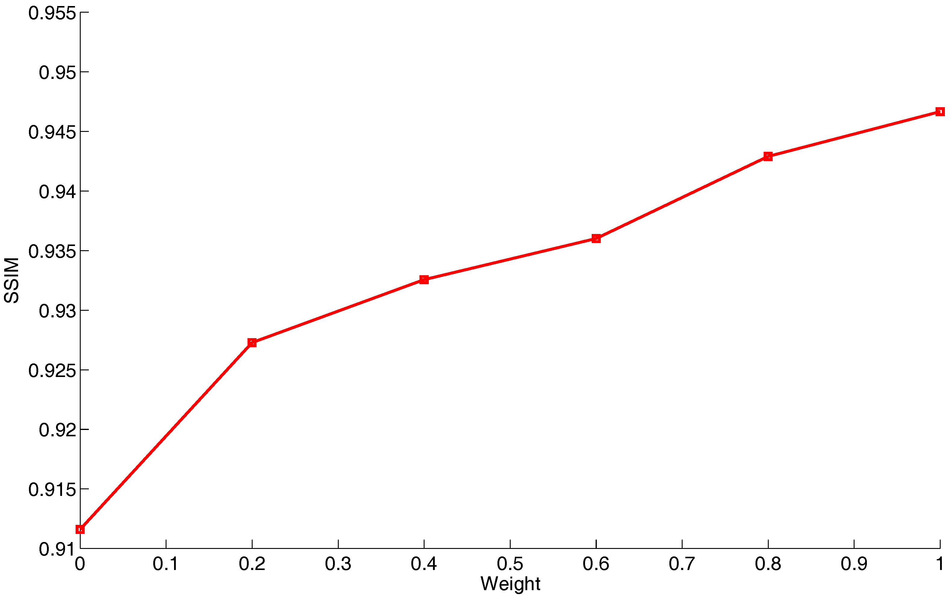
where and denote the intensity values of in and , respectively. Obviously, if we set , only the CNN-based energy cost term is used to detect the seamlines, and if we set , only the intensity difference term is applied to detect the seamlines. In this experiment, we modified the value of this balancing coefficient to illustrate the effectiveness of our defined CNN-based energy cost term. Of course, when we set , our proposed approach is used to detect the seamlines. In Figure 7, we present the seamline detection results generated by different weight settings as , , and . From the whole seamline detection results and especially the detailed local regions shown in Figure 7, we observed that the seamlines detected with the use of CNN-based energy terms are much better than the seamline detected without its use. Noticeably, in the enlarged region, the seamline crosses two buildings instead of nearby roads when the weight was set as , as shown in the left column of Figure 7, due to the fact that the roofs of these two buildings are smooth as well as nearby roads. However, when we set the weight as or , the seamlines successfully rounded these two buildings as expected and chose to cross nearby roads when the CNN-based energy term was considered. In addition, we also applied the SSIM index to quantitatively measure the qualities of seamlines detected by using different weights, and the quality curve is demonstrated in Figure 8. From this quality curve, we observed that, as the value of the weight w increased, the quality of the detected seamline becomes more higher. From this experiment, we convincingly proved that our proposed CNN-based energy cost is effective.
5.2. Comparative Evaluation
In this section, to illustrate the difference between our proposed approach and the state-of-the-art one proposed by Li et al. [5] more clearly, we conducted the experiment on four adjacent images in the first strip of the Vaihingen dataset. We compared these two approaches to prove the superiority of our proposed approach, and illustrated why our approach outperforms the approach proposed by [5]. Then, we also give the quality evaluations of the seamlines detected by two approaches by using both the traditional measurement and the quantitative one. In addition, we also compared our proposed approach with Dijkstra’s approach [39] and OrthoVista [40]. OrthoVista is one of the most popularly used commercial software programs.
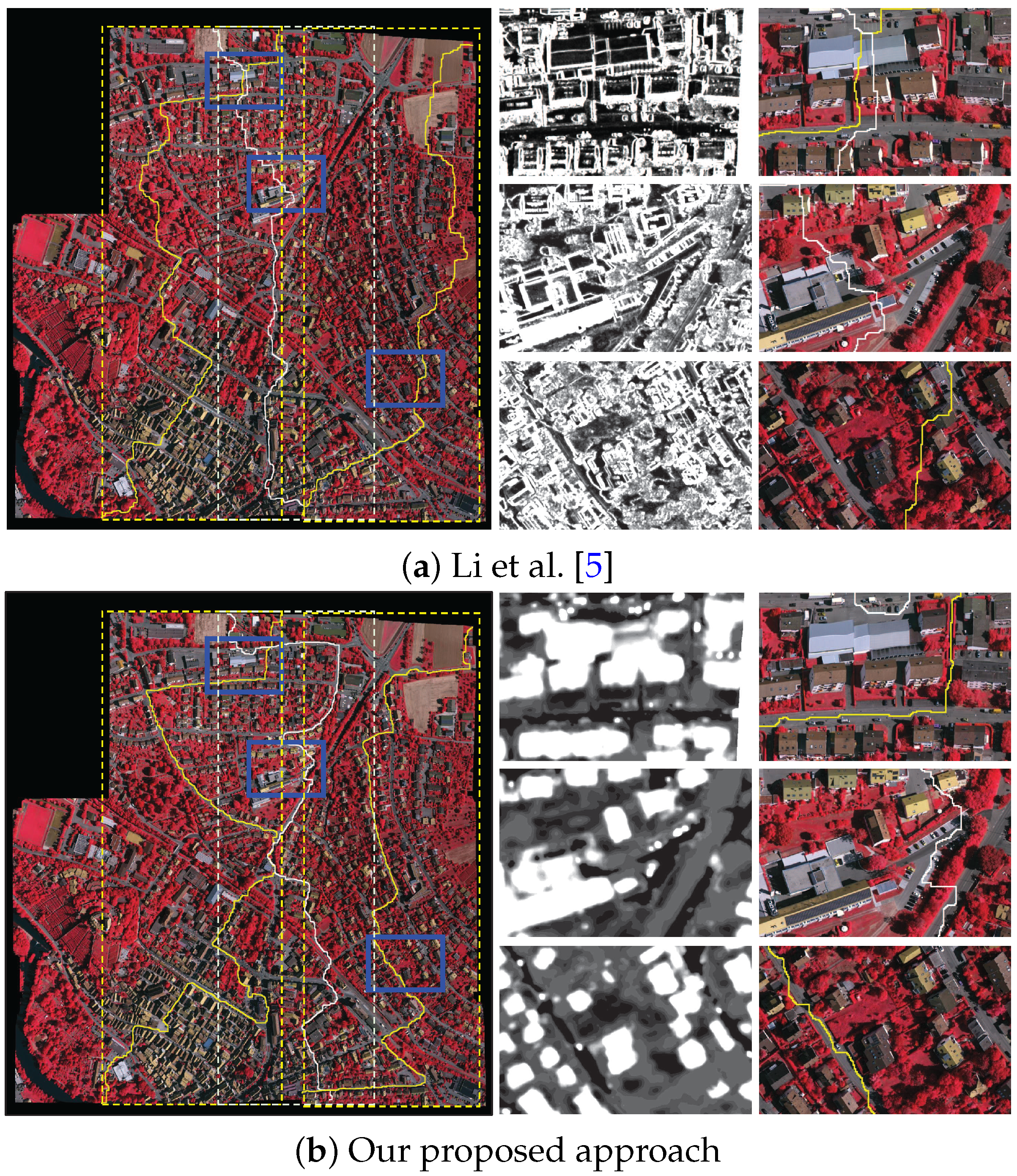
The seamline detection results generated by Li et al. [5] and our proposed approach are shown in Figure 9a,b, respectively. From the whole seamline detection results and especially the detailed local regions, we observed that the seamlines detected by our proposed approach is much better than the seamlines detected by Li et al. [5]. For example, in three local regions, the seamlines detected by our proposed approach all avoid crossing the buildings, and choose to pass through nearby roads, but the seamlines detected by Li et al. [5] fail to bypass those obvious objects. To illustrate the reason of this problem more clear, we also presented the corresponding normalized energy cost maps of local enlarged regions in the middle column of Figure 9a,b. We found that the energy cost maps generated by our approach are more reasonable, which can distinguish the obvious objects from the background more better. In addition, we can find out why the seamlines presented in Figure 9a cross those buildings. For example, in the first local region, the energy costs of two buildings crossed by the seamlines are very small due to the fact that the roofs of these two buildings are very smooth. However, in the energy cost map generated by our proposed semantic-based approach, the energy costs of those two buildings are so large that the seamlines would avoid crossing them. For the second and third local regions, the similar reason can be used to illustrate why the seamlines detected by Li et al. [5] fail to bypass those buildings, but our seamlines avoid crossing them.
In addition, we present the seamline detection results generated by Dijkstra’s approach [39] and OrthoVista in Figure 10. We can find that our proposed approach also outperforms Dijkstra’s approach and OrthoVista. From the local enlarged regions, we observed that the seamlines detected by OrthoVista cannot avoid crossing obvious objects in some cases. In total, those seamlines cross 21 buildings and 17 cars, but the seamlines detected by our approach only cross two cars. We also observed that the seamlines generated by Dijkstra’s approach can avoid crossing major obvious objects as our approach does. However, they also cross two buildings and two cars.
In addition, to prove the superiority of our proposed approach more powerful, some statistical results of those seamlines generated by four approaches are presented in Table 3. In the second column, we presented the results of the traditional quality measurement, namely, the numbers of obvious objects passed through, and we found that the seamlines generated by Li et al.’s approach cross 15 buildings and two cars, but the seamlines detected by our proposed approach successfully avoid crossing the buildings, and only cross two cars. In addition, we also evaluated those seamlines by using the quantitative quality measurement defined in Section 4, which can provide an objective evaluation, as shown in the third column of Table 3. We found that the score of our seamlines is 0.9585, which is much larger than the scores of the seamlines generated by the rest three approaches. From those two quality measurements, we proved that our proposed optimal seamline detection approach outperforms the state-of-the-art approaches and commercial software.
In the aspect of computational time, as shown in the last column of Table 3, the approach proposed by Li et al. [5] took around 65.31 s, consisting of all the elapsed times in energy computation and graph cuts optimization. Our proposed approach took around 80.89 s, not only including energy definition and graph cuts optimization, but also including semantic segmentation (27.19 s). Therefore, the time of seamline detection via graph cuts is just 53.70 s. Dijkstra’s approach took around 96.281 s, which is the longest one. In addition, OrthoVista took around 50 s.
In conclusion, in this experiment, we firstly made the comparison between two approaches step-by-step: one is our approach, and the other is one of the state-of-the-art approaches [5]. From the comparative experimental results, we found that our approach can generate more better seamlines than this state-of-the-art approach, and just a little time-consuming than this approach due to the fact that we need to do semantic segmentation in advance. From this visual comparison, we also can find that the energy cost map defined by our proposed CNN-based approach is more reasonable than the energy map defined by [5], which is the main reason why our approach performs better than [5]. In addition, we also proved that our proposed approach is better than Dijkstra’s approach and OrthoVista too.
5.3. More Comparative Experiments
To prove that our proposed approach can handle more types of aerial images, we firstly tested our proposed approach on the images captured from San Francisco, namely, the second dataset. In this dataset, we manually classified those training images into six object classes as a typical example shown in Figure 11. We selected two groups of images from this dataset to test our proposed approach and compared it with Li et al.’ approach, Dijkstra’s approach [39] and OrthoVista. The first group is comprised of three adjacent images, and the second group is comprised of four adjacent images.
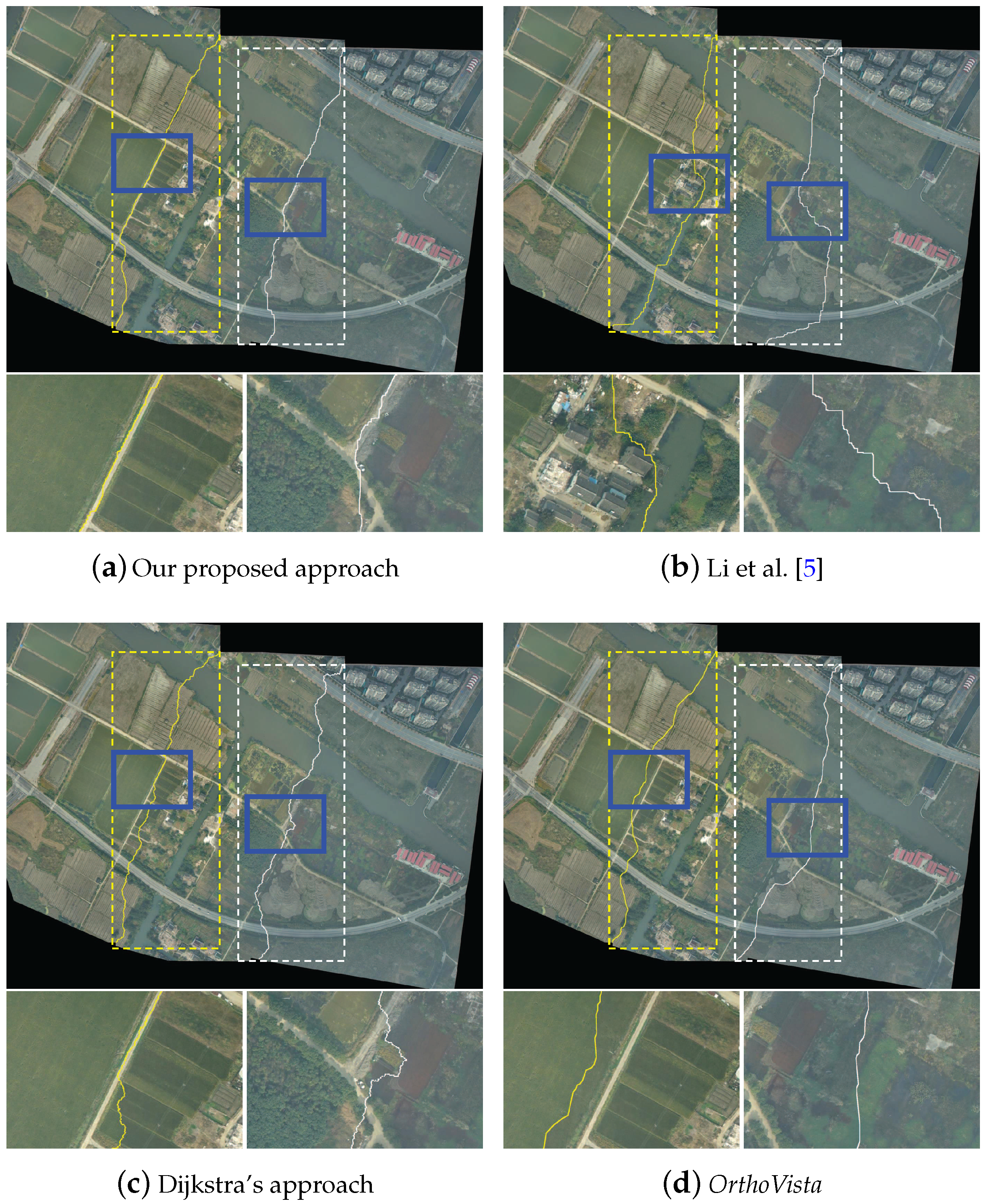
Figure 12 shows the seamline detection results of the first group of images. We found that the seamlines detected by Li et al., approach, Dijkstra’s approach and OrthoVista all cross many buildings, as shown in Figure 12b–d, especially in the enlarged detailed regions. However, the seamlines detected by our proposed approach successfully avoid crossing those buildings and choose to cross the nearby roads, as shown in Figure 12a. The seamlines detected by our approach also cross some buildings, but all of them are located on the endpoint regions of the seamlines whose endpoints are formed by the overlapped intersection. Those buildings are also crossed by the seamlines detected by those three approaches and software. The seamline detection results of the second group of images are shown in Figure 13. Similar conclusions can be drawn. Namely, our proposed approach outperforms the Li et al. approach, Dijkstra’s approach and OrthoVista, and the seamlines detected by our approach can round most buildings crossed by the seamlines detected by those state-of-the-art approaches and software.
In addition, we also tested our proposed approach on the images captured from one non-urban area. We selected three adjacent images from this dataset to test our proposed approach. Noticeably, we have not generated the ground truth images for this dataset. In addition, we applied the trained model of the second dataset to do semantic segmentation for this non-urban dataset. In addition, we found that our proposed approach also can generate high-quality seamlines for non-urban area, as shown in Figure 14a. In addition, we also can find that the rest of the three approaches can also detect high-quality seamlines, as shown in Figure 14b–d, because only a few obvious objects exist in this non-urban area.
At last, we present the detailed statical results of those seamlines generated by four approaches in Table 4. From Table 4, we can easily find that the seamlines generated by our approach cross the least obvious objects in all experiments by comparing with Li et al.’s approach, Dijkstra’s approach and OrthoVista. In addition, the buildings crossed by our approach are located on the endpoint regions. Those buildings are very difficult to bypass. We also applied the SSIM index to evaluate the qualities of detected seamlines. The results of quantitative evaluation also show that our seamlines have highest scores in all experiments, as shown in the third column of Table 4. In the aspect of computation time, the computational times of four approaches are almost the same, and they are all at the same level, as shown in the last column of Table 4.
6. Conclusions
In this paper, we proposed a novel optimal seamline detection approach with the use of the CNN-based semantic image segmentation and a graph cuts energy minimization framework. In this algorithm, the overlap regions of two input aligned images are first classified based on the trained full convolutional network independently. Then, the energy cost of each pixel is designed by combing the probabilities of belonging to each class provided by the semantic segmentation network. Finally, the graph cuts energy optimization algorithm is used to find the solution with the minimum energy, and the seamline is determined at the same time. The energy costs which represent the differences along the seamline are only defined based on the classified results of the semantic segmentation network, instead of being defined by combing several features, which means that we don’t need to design features for seamline detection anymore—we learn it. In addition, the learned semantic informations are fully used to guide the process of optimal seamline detection. To further prove the superiority of our proposed approach, we applied the images captured from Vaihingen, San Francisco and one small town of China to compare our approach with two state-of-the-art approaches [5,39] and one popularly used commercial software OrthoVista. By comparing with those two state-of-the-art approaches and one commercial software program, we found that our proposed approach demonstrates a significant advantage in avoiding the seamlines crossing obvious objects.
Nevertheless, the proposed algorithm may be improved in the future in the following ways. First, more training datasets should be prepared to train our fully convolutional network. Second, the superpixel segmentation can be introduced to greatly improve the optimization efficiency by decreasing the number of elements in graph cuts. Last but not least, the seamline network optimization framework [20,39,41] can be combined with our approach to produce a complete image mosaic from a large set of images automatically.
Acknowledgments
This work was partially supported by the National Natural Science Foundation of China (Project No. 41571436), the Hubei Province Science and Technology Support Program, China (Project No. 2015BAA027), the National Natural Science Foundation of China under Grant 91438203, LIESMARS Special Research Funding, and the South Wisdom Valley Innovative Research Team Program.
Author Contributions
Li Li and Jian Yao conducted the algorithm design, and Li Li wrote the paper and performed all the experiments under the supervision of Jian Yao. Yahui Liu designed and trained the deep convolutional neural network. Wei Yuan and Shuzhu Shi contributed to prepare and analyze the experimental data. Shenggu Yuan contributed to prepare the compared results. All authors were involved in modifying the paper, the literature review and the discussion of the results.
Conflicts of Interest
The authors declare no conflict of interest.
References
- Chon, J.; Kim, H.; Lin, C.S. Seam-line determination for image mosaicking: A technique minimizing the maximum local mismatch and the global cost. ISPRS J. Photogramm. Remote Sens. 2010, 65, 86–92. [Google Scholar] [CrossRef]
- Yu, L.; Holden, E.J.; Dentith, M.C.; Zhang, H. Towards the automatic selection of optimal seam line locations when merging optical remote-sensing images. Int. J. Remote Sens. 2012, 33, 1000–1014. [Google Scholar] [CrossRef]
- Wan, Y.; Wang, D.; Xiao, J.; Lai, X.; Xu, J. Automatic determination of seamlines for aerial image mosaicking based on vector roads alone. ISPRS J. Photogramm. Remote Sens. 2013, 76, 1–10. [Google Scholar] [CrossRef]
- Pan, J.; Zhou, Q.; Wang, M. Seamline determination based on segmentation for urban image mosaicking. IEEE Trans. Geosci. Remote Sens. Lett. 2014, 11, 1335–1339. [Google Scholar] [CrossRef]
- Li, L.; Yao, J.; Lu, X.; Tu, J.; Shan, J. Optimal seamline detection for multiple image mosaicking via graph cuts. ISPRS J. Photogramm. Remote Sens. 2016, 113, 1–16. [Google Scholar] [CrossRef]
- Kerschner, M. Seamline detection in colour orthoimage mosaicking by use of twin snakes. ISPRS J. Photogramm. Remote Sens. 2001, 56, 53–64. [Google Scholar] [CrossRef]
- Soille, P. Morphological image compositing. IEEE Trans. Pattern Anal. Mach. Intell. 2006, 28, 673–683. [Google Scholar] [CrossRef] [PubMed]
- Li, L.; Yao, J.; Xie, R.; Xia, M.; Zhang, W. A unified framework for street-view panorama stitching. Sensors 2016, 17, 1. [Google Scholar] [CrossRef] [PubMed]
- Gracias, N.; Mahoor, M.; Negahdaripour, S.; Gleason, A. Fast image blending using watersheds and graph cuts. Image Vis. Comput. 2009, 27, 597–607. [Google Scholar] [CrossRef]
- Agarwala, A.; Dontcheva, M.; Agrawala, M.; Drucker, S.; Colburn, A.; Curless, B.; Salesin, D.; Cohen, M. Interactive digital photomontage. ACM Trans. Gr. (TOG) 2004, 23, 294–302. [Google Scholar] [CrossRef]
- Chandelier, L.; Martinoty, G. Radiometric aerial triangulation for the equalization of digital aerial images and orthoimages. Photogramm. Eng. Remote Sens. 2009, 75, 193–200. [Google Scholar] [CrossRef]
- Pan, J.; Wang, M.; Li, D.; Li, J. A network-based radiometric equalization approach for digital aerial orthoimages. IEEE Geosci. Remote Sens. Lett. 2010, 7, 401–405. [Google Scholar] [CrossRef]
- Kass, M.; Witkin, A.; Terzopoulos, D. Snakes: Active contour models. Int. J. Comput. Vis. 1988, 1, 321–331. [Google Scholar] [CrossRef]
- Dijkstra, E.W. A note on two problems in connexion with graphs. Numer. Math. 1959, 1, 269–271. [Google Scholar] [CrossRef]
- Bellman, R. Dynamic Programming; Princeton University Press: Princeton, NJ, USA, 1957. [Google Scholar]
- Boykov, Y.; Veksler, O.; Zabih, R. Fast approximate energy minimization via graph cuts. IEEE Trans. Pattern Anal. Mach. Intell. 2001, 23, 1222–1239. [Google Scholar] [CrossRef]
- Wang, L.; Ai, H.; Zhang, L. Automated seamline detection in orthophoto mosaicking using improved snakes. In Proceedings of the International Conference on Information Engineering and Computer Science (ICIECS), Wuhan, China, 25–26 December 2010; pp. 1–4. [Google Scholar]
- Pan, J.; Wang, M.; Li, J.; Yuan, S.; Hu, F. Region change rate-driven seamline determination method. ISPRS J. Photogramm. Remote Sens. 2015, 105, 141–154. [Google Scholar] [CrossRef]
- Wang, M.; Yuan, S.; Pan, J.; Fang, L.; Zhou, Q.; Yang, G. Seamline determination for high resolution orthoimage mosaicking using watershed segmentation. Photogramm. Eng. Remote Sens. 2016, 82, 121–133. [Google Scholar] [CrossRef]
- Chen, Q.; Sun, M.; Hu, X.; Zhang, Z. Automatic seamline network generation for urban orthophoto mosaicking with the use of a digital surface Model. Remote Sens. 2014, 6, 12334–12359. [Google Scholar] [CrossRef]
- Pang, S.; Sun, M.; Hu, X.; Zhang, Z. SGM-based seamline determination for urban orthophoto mosaicking. ISPRS J. Photogramm. Remote Sens. 2016, 112, 1–12. [Google Scholar] [CrossRef]
- Floyd, R. Algorithm 97: Shortest path. Commun. ACM 1962, 5, 345. [Google Scholar] [CrossRef]
- Zeng, L.; Zhang, S.; Zhang, J.; Zhang, Y. Dynamic image mosaic via SIFT and dynamic programming. Machine Vis. Appl. 2014, 25, 1271–1282. [Google Scholar] [CrossRef]
- Kwatra, V.; Schödl, A.; Essa, I.; Turk, G.; Bobick, A. Graphcut textures image and video synthesis using graph cuts. ACM Trans. Gr. (TOG) 2003, 22, 277–286. [Google Scholar] [CrossRef]
- Boykov, Y.; Kolmogorov, V. An experimental comparison of min-cut/max-flow algorithms for energy minimization in vision. IEEE Trans. Pattern Anal. Mach. Intell. 2004, 26, 1124–1137. [Google Scholar] [CrossRef] [PubMed]
- Long, J.; Shelhamer, E.; Darrell, T. Fully convolutional networks for semantic segmentation. In Proceedings of the IEEE Conference on Computer Vision and Pattern Recognition, Cambridge, MA, USA, 7–12 June 2015; pp. 3431–3440. [Google Scholar]
- Simonyan, K.; Zisserman, A. Very deep convolutional networks for large-scale image recognition. arXiv, 2014; arXiv:1409.1556. [Google Scholar]
- Ioffe, S.; Szegedy, C. Batch normalization: Accelerating deep network training by reducing internal covariate shift. arXiv, 2015; arXiv:1502.03167. [Google Scholar]
- Nair, V.; Hinton, G.E. Rectified linear units improve restricted boltzmann machines. In Proceedings of the International Conference on Machine Learning (ICML), Haifa, Israel, 21–24 June 2010; pp. 807–814. [Google Scholar]
- Jia, Y.; Shelhamer, E.; Donahue, J.; Karayev, S.; Long, J.; Girshick, R.; Guadarrama, S.; Darrell, T. Caffe: Convolutional architecture for fast feature embedding. In Proceedings of the 22nd ACM International Conference on Multimedia, Orlando, FL, USA, 3–7 November 2014; pp. 675–678. [Google Scholar]
- Bottou, L. Large-scale machine learning with stochastic gradient descent. In Proceedings of the COMPSTAT, Paris, France, 22–27 August 2010; pp. 177–186. [Google Scholar]
- Badrinarayanan, V.; Handa, A.; Cipolla, R. SegNet: A deep convolutional encoder-decoder architecture for robust semantic pixel-wise labelling. arXiv, 2015; arXiv:1505.07293. [Google Scholar]
- Eigen, D.; Fergus, R. Predicting depth, surface normals and semantic labels with a common multi-scale convolutional architecture. In Proceedings of the IEEE International Conference on Computer Vision (ICCV), Los Alamitos, CA, USA, 7–13 December 2015; pp. 2650–2658. [Google Scholar]
- Wang, Z.; Bovik, A.C.; Sheikh, H.R.; Simoncelli, E.P. Image quality assessment: From error visibility to structural similarity. IEEE Trans. Image Process. 2004, 13, 600–612. [Google Scholar] [CrossRef] [PubMed]
- Xu, W.; Mulligan, J. Performance evaluation of color correction approaches for automatic multi-view image and video stitching. In Proceedings of the IEEE Conference on Computer Vision and Pattern Recognition (CVPR), San Francisco, California, USA, 13–18 June 2010; pp. 263–270. [Google Scholar]
- Qureshi, H.; Khan, M.; Hafiz, R.; Cho, Y.; Cha, J. Quantitative quality assessment of stitched panoramic images. IET Image Process. 2012, 6, 1348–1358. [Google Scholar] [CrossRef]
- Dissanayake, V.; Herath, S.; Rasnayaka, S.; Seneviratne, S.; Vidanaarachchi, R.; Gamage, C. Quantitative and Qualitative Evaluation of Performance and Robustness of Image Stitching Algorithms. In Proceedings of the International Conference on Digital Image Computing: Techniques and Applications (DICTA), Adelaide, Australia, 23–25 November 2015; pp. 1–6. [Google Scholar]
- 2D Semantic Labeling Contest. Available online: http://www2.isprs.org/commissions/comm3/wg4/semantic-labeling.html (accessed on 7 July 2017).
- Pan, J.; Wang, M.; Ma, D.; Zhou, Q.; Li, J. Seamline network refinement based on area Voronoi diagrams with overlap. IEEE Trans. Geosci. Remote Sens. 2014, 52, 1658–1666. [Google Scholar] [CrossRef]
- Trimble. Available online: http://www.trimble.com/ (accessed on 7 July 2017).
- Mills, S.; McLeod, P. Global seamline networks for orthomosaic generation via local search. ISPRS J. Photogramm. Remote Sens. 2013, 75, 101–111. [Google Scholar] [CrossRef]
Figure 1.
The overview of our proposed optimal seamline detection approach.

Figure 2.
An illustration of our proposed pixel-to-pixel architecture. There are no fully connected layers in our architecture, only convolutional layers.
Figure 2.
An illustration of our proposed pixel-to-pixel architecture. There are no fully connected layers in our architecture, only convolutional layers.

Figure 3.
A demonstration of the training sample: (left) the original image; (right) the manually labeled ground truth map in which different object classes are marked with different colors, e.g., buildings with blue, cars with yellow, trees with green, low vegetation with cyan, water with red and impervious surface with white.

Figure 4.
An illustration of side-output predictions.
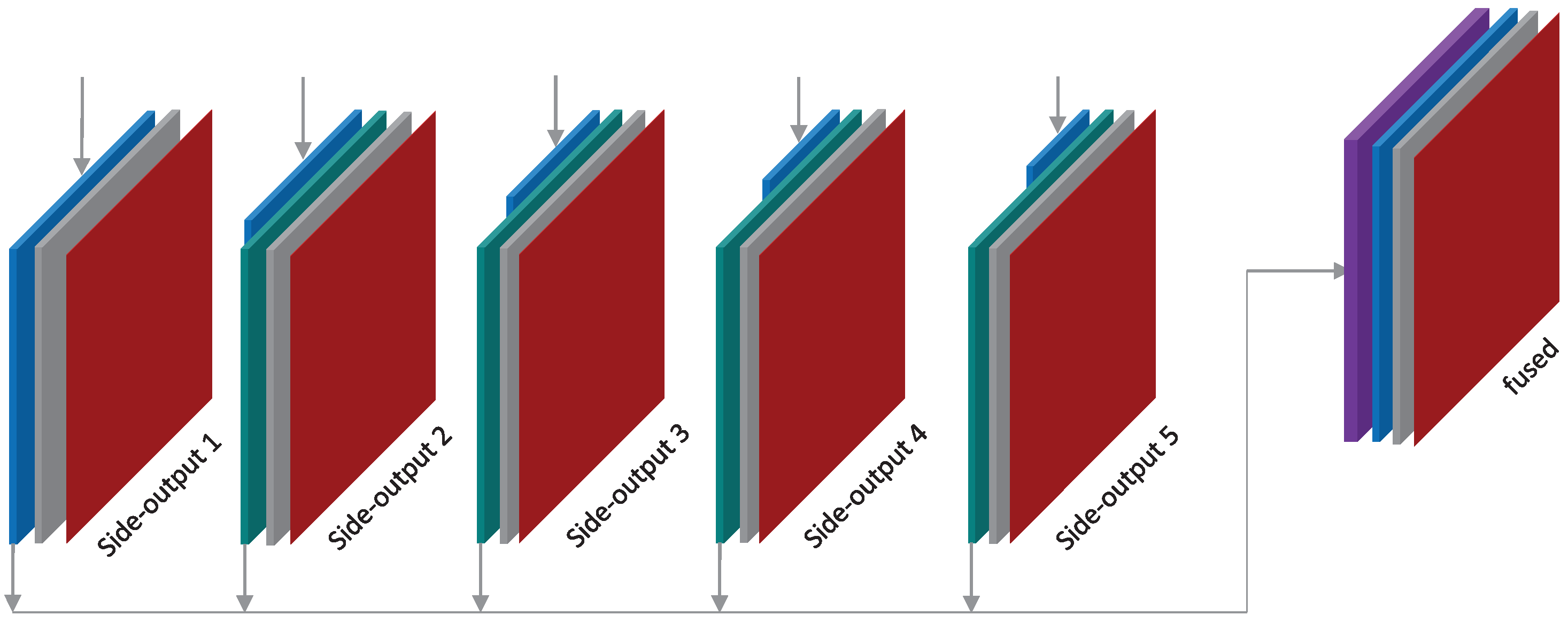
Figure 5.
The comparison between the algorithm proposed by [5] and our proposed method in the term of the energy cost map: (a,b) the cropped regions of two input aligned images; (c) the energy cost map generated by [5]; (d) the energy cost map generated by our proposed CNN-based method. The lighter regions indicate higher energy costs in (c,d), where the seamline avoids to cross.
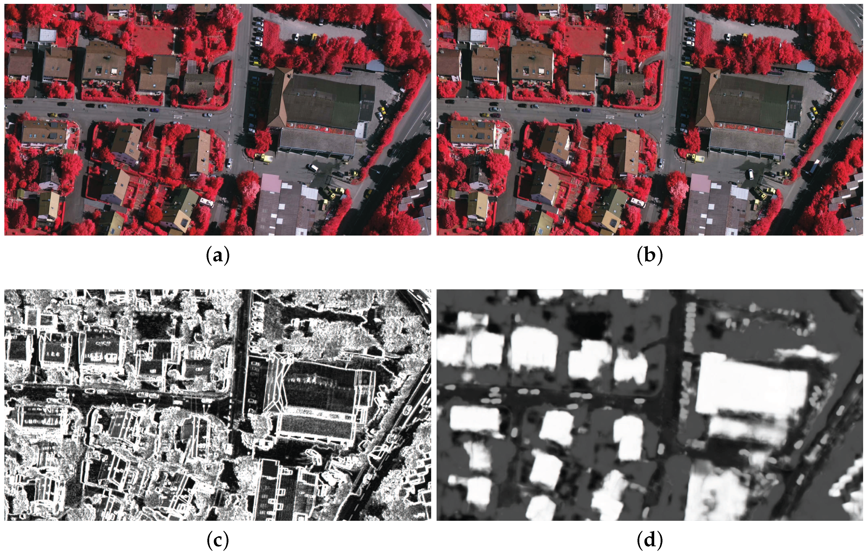
Figure 6.
An illustration example of detecting the optimal seamline between two images via graph cuts. The thickness of lines between adjacent pixels represents the value of the energy cost and the “cut” denotes the minimum cut, which means the optimal seamline.
Figure 6.
An illustration example of detecting the optimal seamline between two images via graph cuts. The thickness of lines between adjacent pixels represents the value of the energy cost and the “cut” denotes the minimum cut, which means the optimal seamline.
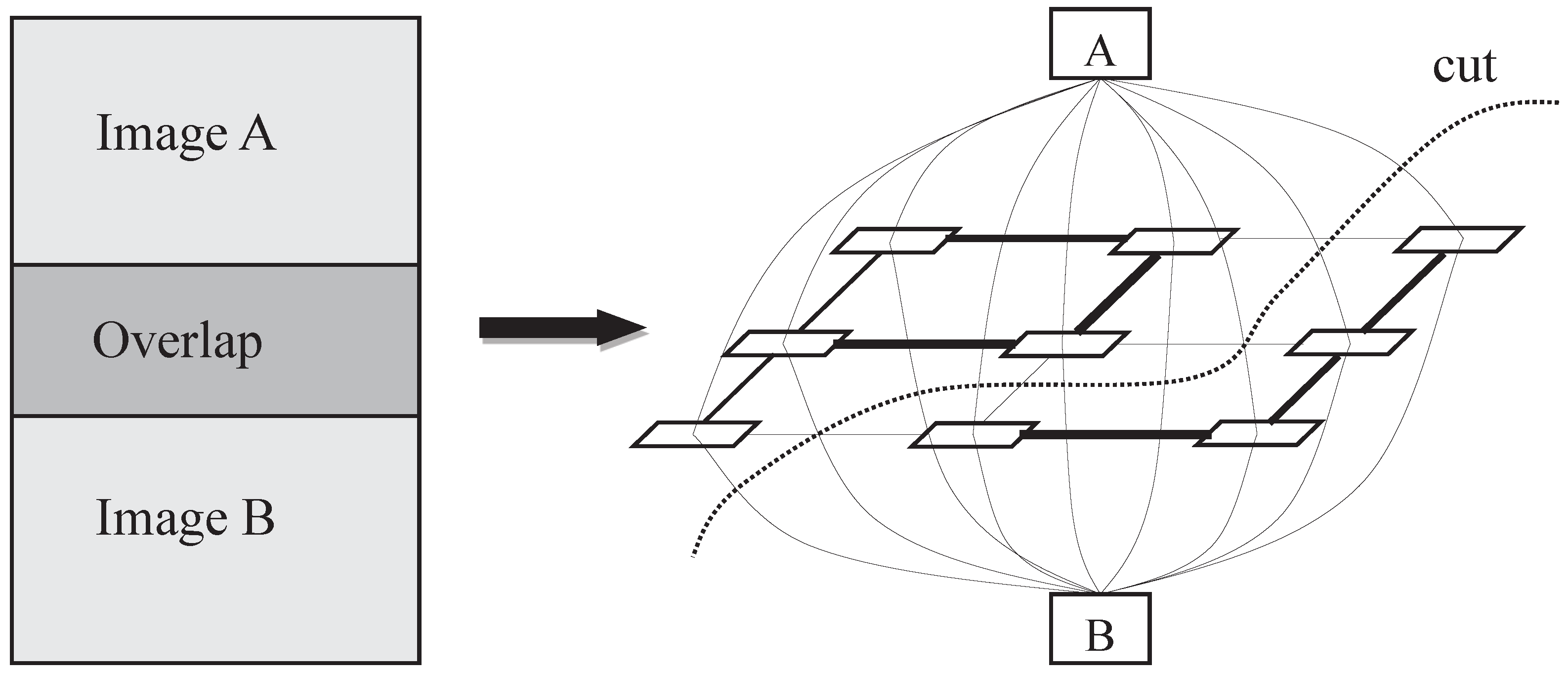
Figure 7.
The seamline detection results generated by using different weights: , , and from left to right. The dash boxes represent the overlapped regions between input images.
Figure 7.
The seamline detection results generated by using different weights: , , and from left to right. The dash boxes represent the overlapped regions between input images.
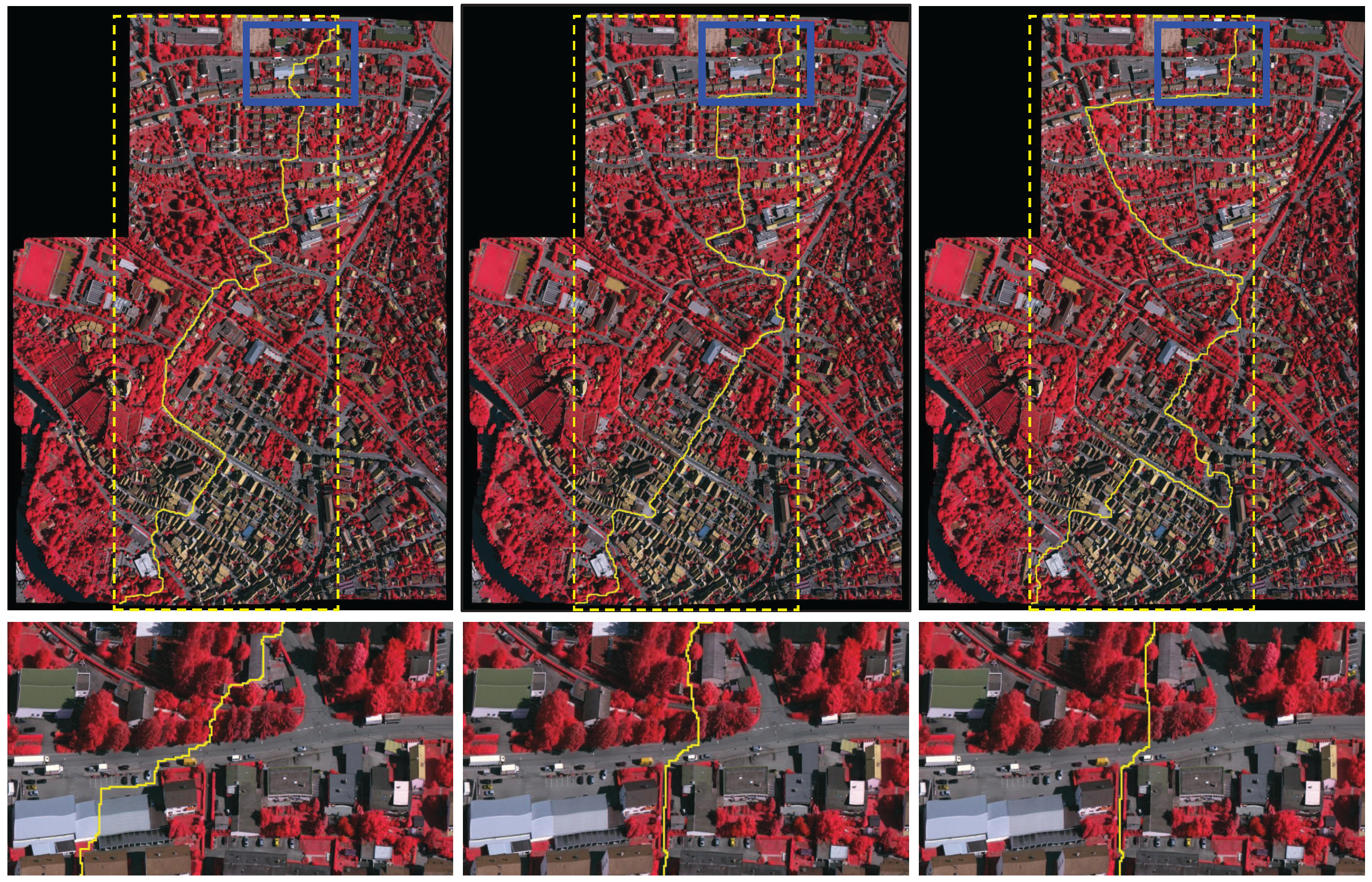
Figure 8.
The curve of quantitative qualities of seamlines detected by using different weights.

Figure 9.
Visual comparison of the seamline detection results generated by Li et al. [5] (a) and our proposed approach (b). In (a) or (b), the left pictures are the stitched images drawn with the detected seamlines, the right pictures are three corresponding local enlarged regions of the stitched images, and the middle pictures are the corresponding normalized energy cost maps of local regions, where the brighter regions indicate higher energy costs. The dash boxes represent the overlapped regions between input images.

Figure 10.
The seamline detection results generated by Dijkstra’s approach (a) and a commercial software OrthoVista (b). The dash boxes represent the overlapped regions between input images. The dash boxes represent the overlapped regions between input images.
Figure 10.
The seamline detection results generated by Dijkstra’s approach (a) and a commercial software OrthoVista (b). The dash boxes represent the overlapped regions between input images. The dash boxes represent the overlapped regions between input images.

Figure 11.
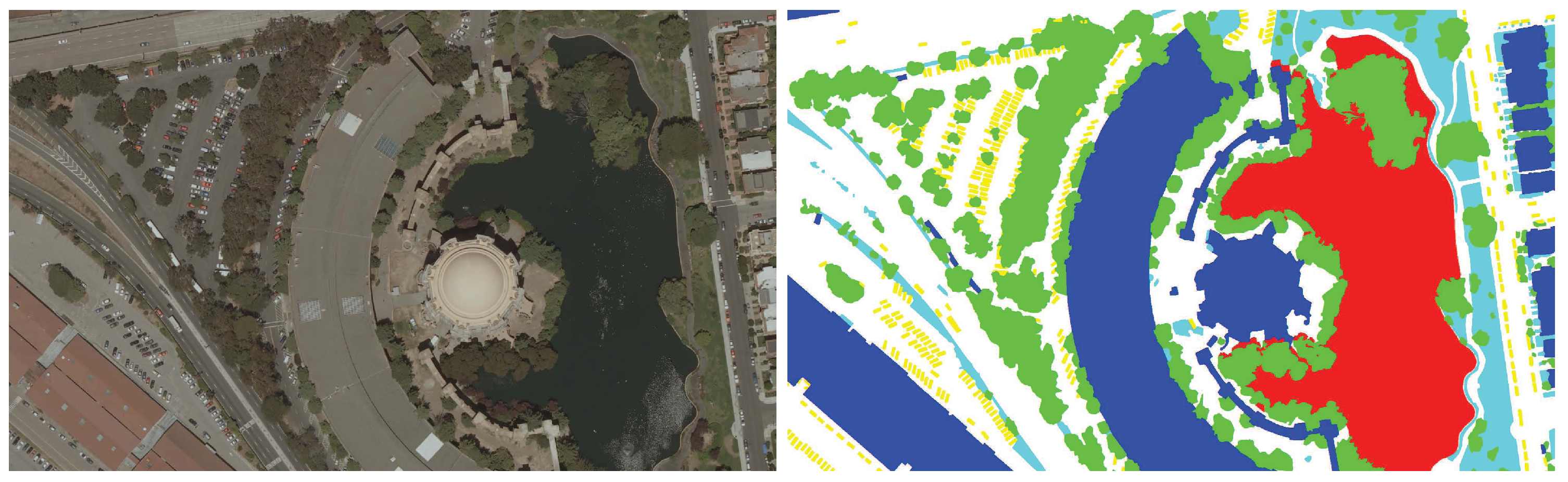
A demonstration of a small example image from the San Francisco dataset: (left) the original image; (right) the corresponding ground truth image classified as buildings (blue), cars (yellow), trees (green), low vegetation (cyan), water (red) and impervious surface (white).
Figure 11.
A demonstration of a small example image from the San Francisco dataset: (left) the original image; (right) the corresponding ground truth image classified as buildings (blue), cars (yellow), trees (green), low vegetation (cyan), water (red) and impervious surface (white).

Figure 12.
The seamlines detected by our proposed approach (a), Li et al. [5] (b), Dijkstra’s approach (c) and OrthoVista (d) on the first group of images. The dash boxes represent the overlapped regions between input images.
Figure 12.
The seamlines detected by our proposed approach (a), Li et al. [5] (b), Dijkstra’s approach (c) and OrthoVista (d) on the first group of images. The dash boxes represent the overlapped regions between input images.
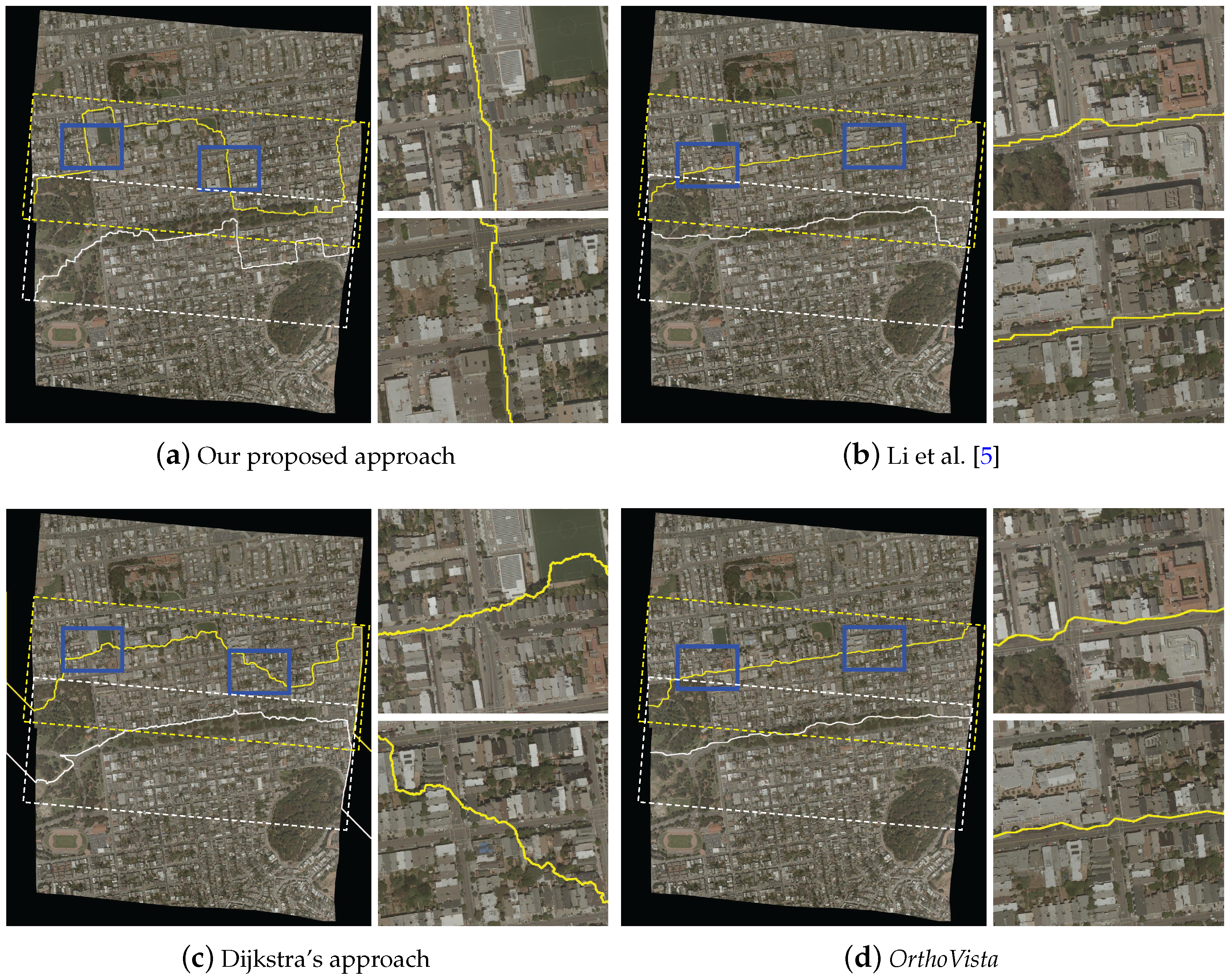
Figure 13.
The seamlines detected by our proposed approach (a); Li et al. [5] (b); Dijkstra’s approach(c) and OrthoVista (d) on the second group of images. The dash boxes represent the overlapped regions between input images.
Figure 13.
The seamlines detected by our proposed approach (a); Li et al. [5] (b); Dijkstra’s approach(c) and OrthoVista (d) on the second group of images. The dash boxes represent the overlapped regions between input images.
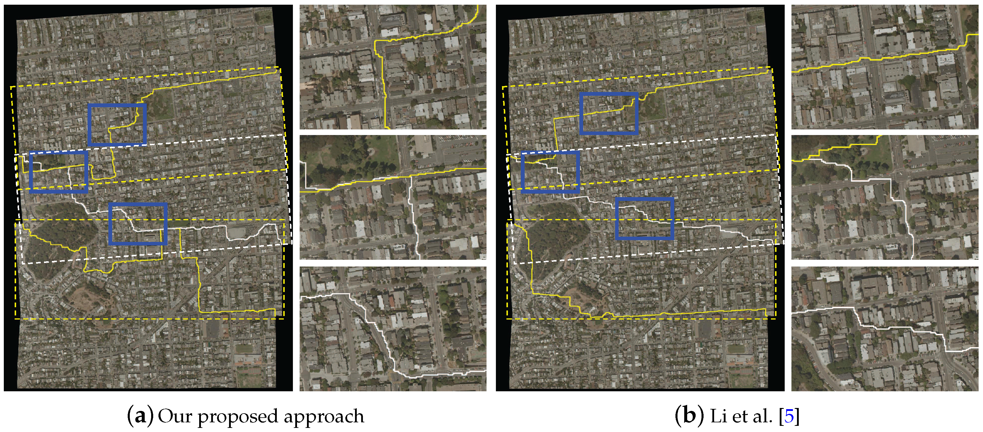
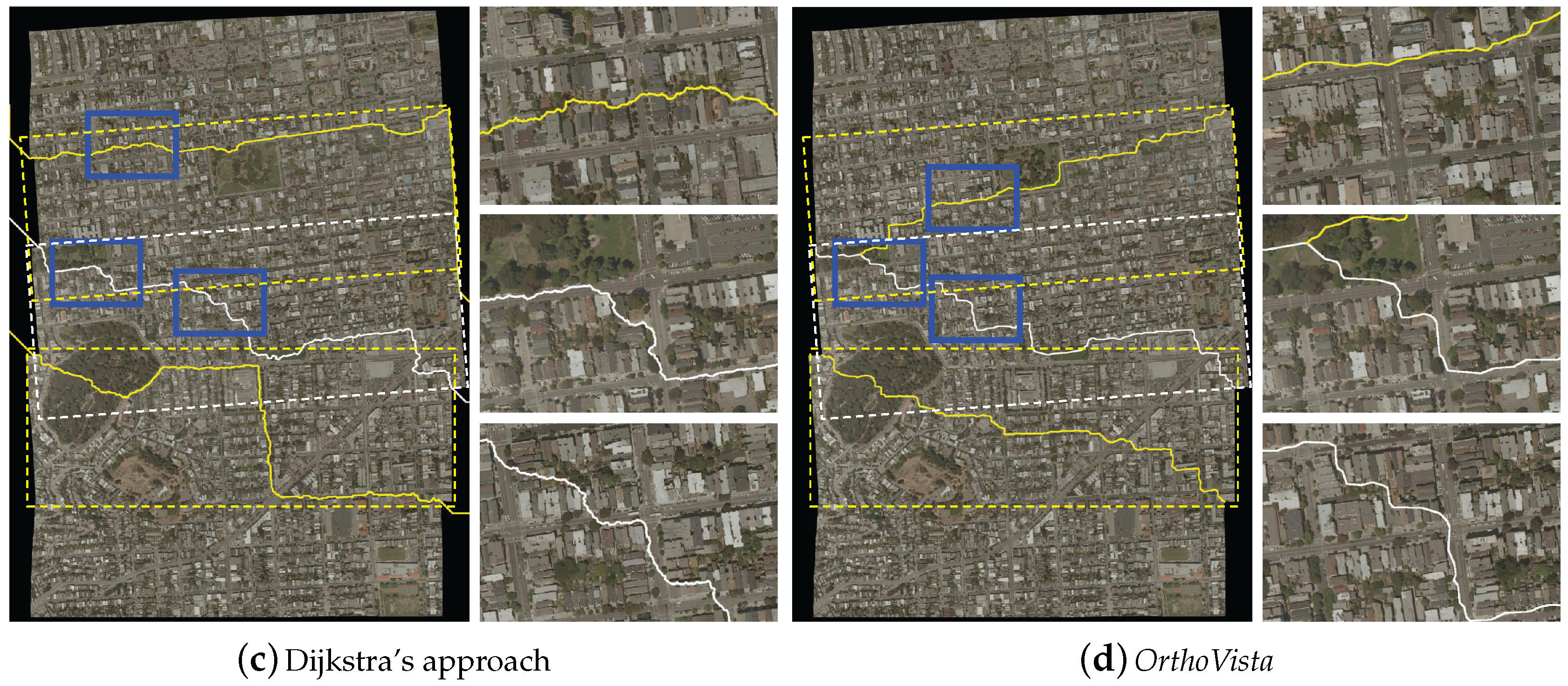
Figure 14.
The seamlines detected by our proposed approach (a); Li et al. [5] (b); Dijkstra’s approach (c) and OrthoVista (d) on one non-urban area. The dash boxes represent the overlapped regions between input images.
Figure 14.
The seamlines detected by our proposed approach (a); Li et al. [5] (b); Dijkstra’s approach (c) and OrthoVista (d) on one non-urban area. The dash boxes represent the overlapped regions between input images.


Table 1.
The penalty coefficients setting of all object classes.
| Building | Car | Tree | Low Vegetation | Water | Impervious Surface | |
|---|---|---|---|---|---|---|
| Penalty Coefficients | 1.0 | 1.0 | 0.3 | 0 | 0 | 0 |
Table 2.
The details of three datasets used in our experiments.
| Descriptions\Dataset | Dataset 1 | Dataset 2 | Dataset 3 |
|---|---|---|---|
| Location | Vaihingen (Germany) | San Francisco (USA) | China |
| Image size | 7680 × 13,824 pixel | 9328 × 6454 | 4535 × 6771 |
| The number of images | 14 | 69 | 53 |
| Spatial resolution | 0.1 m | 0.2 m | 0.2 m |
| Spectral bands | IR-R-G | R-G-B | R-G-B |
| Description of the study area | Small-sized and detached buildings; many surrounding trees; many cars | Densely-distributed buildings; many cars | non-urban area; several buildings; several cars |
Table 3.
The quality assessment of seamlines detected by our proposed approach, the approach proposed by Li et al. [5], Dijkstra’s approach and OrthoVista in the Figure 9 and Figure 10.
| Numbers of Obvious Objects Passed Through | Quantitative Quality (SSIM) | Time(s) | |
|---|---|---|---|
| Our proposed approach | 0 building and 2 cars | 0.9585 | 80.89 |
| Li et al. [5] | 15 buildings and 2 cars | 0.9057 | 65.31 |
| Dijkstra’s approach [39] | 2 buildings and 2 cars | 0.9488 | 96.281 |
| OrthoVista | 21 buildings and 17 cars | 0.8882 | 50 |
Table 4.
The quality assessment of seamlines detected by our proposed approach, the approach proposed by Li et al. [5], Dijkstra’s approach and OrthoVista in Figure 12, Figure 13 and Figure 14
| Figure 12 | Numbers of Obvious Objects Passed Through | Quantitative Quality (SSIM) | Time(s) |
|---|---|---|---|
| Our proposed approach | 2 buildings and 1 cars | 0.8985 | 20.30 |
| Li et al. [5] | 5 buildings and 7 cars | 0.866991 | 15.907 |
| Dijkstra’s approach [39] | 8 buildings and 1 cars | 0.8681 | 21.21 |
| OrthoVista | 5 buildings and 32 cars | 0.8624 | 23 |
| Figure 13 | |||
| Our proposed approach | 6 buildings and 2 cars | 0.8842 | 30.95 |
| Li et al. [5] | 12 buildings and 2 cars | 0.8717 | 31.322 |
| Dijkstra’s approach [39] | 23 buildings and 5 cars | 0.8418 | 33.14 |
| OrthoVista | 27 buildings and 58 cars | 0.8362 | 31 |
| Figure 14 | |||
| Our proposed approach | 1 buildings and 0 cars | 0.9165 | 48.36 |
| Li et al. [5] | 2 buildings and 0 cars | 0.859372 | 42.906 |
| Dijkstra’s approach [39] | 1 buildings and 0 cars | 0.886896 | 49.0135 |
| OrthoVista | 1 buildings and 0 cars | 0.864969 | 42 |
© 2017 by the authors. Licensee MDPI, Basel, Switzerland. This article is an open access article distributed under the terms and conditions of the Creative Commons Attribution (CC BY) license (http://creativecommons.org/licenses/by/4.0/).
Share and Cite
MDPI and ACS Style
Li, L.; Yao, J.; Liu, Y.; Yuan, W.; Shi, S.; Yuan, S. Optimal Seamline Detection for Orthoimage Mosaicking by Combining Deep Convolutional Neural Network and Graph Cuts. Remote Sens. 2017, 9, 701. https://doi.org/10.3390/rs9070701
AMA Style
Li L, Yao J, Liu Y, Yuan W, Shi S, Yuan S. Optimal Seamline Detection for Orthoimage Mosaicking by Combining Deep Convolutional Neural Network and Graph Cuts. Remote Sensing. 2017; 9(7):701. https://doi.org/10.3390/rs9070701
Chicago/Turabian StyleLi, Li, Jian Yao, Yahui Liu, Wei Yuan, Shuzhu Shi, and Shenggu Yuan. 2017. "Optimal Seamline Detection for Orthoimage Mosaicking by Combining Deep Convolutional Neural Network and Graph Cuts" Remote Sensing 9, no. 7: 701. https://doi.org/10.3390/rs9070701
Note that from the first issue of 2016, this journal uses article numbers instead of page numbers. See further details here.