Estimation of Forest Aboveground Biomass in Changbai Mountain Region Using ICESat/GLAS and Landsat/TM Data
by
Hong Chi
1,2,*, 
Guoqing Sun
3,
Jinliang Huang
1,2,
Rendong Li
1,2,
Xianyou Ren
1,2,
Wenjian Ni
4 and
Anmin Fu
5 1
Institute of Geodesy and Geophysics, Chinese Academy of Sciences, Wuhan 430077, China
2
Hubei Key Laboratory for Environment and Disaster Monitoring and Evaluation, Wuhan 430077, China
3
Department of Geographical Sciences, University of Maryland, College Park, MD 20742, USA
4
Institute of Remote Sensing and Digital Earth, Chinese Academy of Sciences, Beijing 100732, China
5
Academy of Forest Inventory and Planning, State Forestry Administration, Beijing 100714, China
*
Author to whom correspondence should be addressed.
Remote Sens. 2017, 9(7), 707; https://doi.org/10.3390/rs9070707
Submission received: 20 June 2017
/
Revised: 4 July 2017
/
Accepted: 4 July 2017
/
Published: 9 July 2017
(This article belongs to the Section Forest Remote Sensing)
Abstract
:Mapping the magnitude and spatial distribution of forest aboveground biomass (AGB, in Mg·ha−1) is crucial to improve our understanding of the terrestrial carbon cycle. Landsat/TM (Thematic Mapper) and ICESat/GLAS (Ice, Cloud, and land Elevation Satellite, Geoscience Laser Altimeter System) data were integrated to estimate the AGB in the Changbai Mountain area. Firstly, four forest types were delineated according to TM data classification. Secondly, different models for prediction of the AGB at the GLAS footprint level were developed from GLAS waveform metrics and the AGB was derived from field observations using multiple stepwise regression. Lastly, GLAS-derived AGB, in combination with vegetation indices, leaf area index (LAI), canopy closure, and digital elevation model (DEM), were used to drive a data fusion model based on the random forest approach for extrapolating the GLAS footprint AGB to a continuous AGB map. The classification result showed that the Changbai Mountain region was characterized as forest-rich in altitudinal vegetation zones. The contribution of remote sensing variables in modeling the AGB was evaluated. Vegetation index metrics account for large amount of contribution in AGB ranges <150 Mg·ha−1, while canopy closure has the largest contribution in AGB ranges ≥150 Mg·ha−1. Our study revealed that spatial information from two sensors and DEM could be combined to estimate the AGB with an R2 of 0.72 and an RMSE of 25.24 Mg·ha−1 in validation at stand level (size varied from ~0.3 ha to ~3 ha).
1. Introduction
Forest play an important role in the global carbon cycle [1]. Deforestation and forest degradation impact the estimation of anthropogenic greenhouse gas emissions and carbon stock in forests [2,3]. Forest carbon stocks that change dynamically over time can be monitored through regular mapping of the total forest aboveground biomass (AGB, in Mg·ha−1) [3,4,5]. Therefore, mapping the magnitude and spatial distribution of forest AGB is necessary for improving estimates of terrestrial carbon sources and sinks. The traditional methods to estimate forest AGB is based on field measurements or long-term forest inventories; these methods can obtain good AGB estimation. National inventories (e.g., National Forest Resource Inventory Program of the State Forestry Administration, China, or the U.S. Forest Service Inventory and Analysis Program) provided the most detailed field estimates of forest AGB at the national scale [6,7]. However, the lack of field measurements in remote areas and the inconsistency of data requirements among different administrative units are the major constraints to obtain sufficient regional AGB estimation using field-based methods [5,8]. In addition, obtaining comprehensive, spatially-complete, temporally uniform, and accurate forest inventory data is usually time-consuming and labor-intensive over very large areas. Reducing the uncertainty in the AGB estimates requires spatially-continuous observations that are fine enough to capture the variability over a landscape that may undergo natural disturbances or landuse changes [5,9].
Remote sensing has the capability to map forest AGB over wide geographical areas. However, as no remote sensor has been developed that is capable of providing direct measurement of AGB, additional field-sampled AGB is required to correlate with canopy reflectance measured by passive optical sensors or backscatter intensity from Synthetic Aperture Radar (SAR) sensors from moderate to fine spatial resolution [10]. Optical sensor data are appropriate for the retrieval of forest horizontal structures, such as forest types and canopy cover, due to its spectral sensitivity to different species [11]. Furthermore, satellite-based optical sensors are perceptive to other forest structural variables, such as species abundance [12], basal area [13], stem density [13], and crown size [14], which are correlated to some degree with AGB because forest spectral reflectance contains information on the vegetation chlorophyll absorption bands in the visible region and sustained high reflectance in the near-infrared region [15]. Previous studies have demonstrated the sensitivity of visible and shortwave infrared wavelengths to AGB [4,16,17,18]. In addition to the usage of single-band spectral signatures, various vegetation indices (VIs) derived from TM (Thematic Mapper), ETM+ (Enhanced Thematic Mapper Plus), MODIS (Moderate Resolution Imaging Spectroradiometer), etc., as primary data sources have been used to estimate forest AGB in different regions, such as tropical America and Asia, Central Europe, East Africa, the U.S., and China [16,18,19,20,21]. Moreover, some optical sensor data, such as IKONOS, ALOS/PRISM (Advanced Land Observation Satellite/Panchromatic Remote-sensing Instrument for Stereo Mapping), and ZY-3 (Zi Yuan 3), provide a stereo-imaging capability that can be used to predict forest canopy structure [22,23,24]. Although passive optical remote sensing is widely used for AGB estimation, frequent cloud coverage in mountains and moist regions, and the low saturation level of spectral signatures on AGB estimation in medium to high AGB forest (i.e., the spectral reflectance or vegetation index of optical remote-sensing sensors are of limited value in medium to high biomass forests) are the major disadvantages of this technology [11,25,26].
Recently, much attention has been paid to the use of LiDAR (Light Detection And Ranging) remote sensing in AGB estimation due to its potential to capture the vertical structure of vegetation in great detail and it is the only sensor type available at present whose signal does not saturate in high AGB forests (e.g., 1200 Mg·ha−1 and 1300 Mg·ha−1) [27,28,29,30]. LiDAR footprints may be used as a manner of sampling similar to field plots, wherein the derived AGB is used to integrate optical remotely-sensed data in order to facilitate stratification, thereby extending plot-level AGB to large areas [31]. Airborne LiDAR provides highly accurate AGB estimates [32,33,34], but the associated large data volume, as well as the sophisticated technical equipment and high acquisition costs to observe remote areas, usually limit its application at regional and global scales [16]. The Geoscience Laser Altimeter System (GLAS) sensor onboard the Ice, Cloud, and land Elevation satellite(ICESAT) satellite provided data freely and has proven itself suitable for AGB and canopy height estimation over continental-to-global areas [3,4,35,36,37]. One major limitation of GLAS was the lack of imaging capability and the fact that it provided relatively sparse sampling information on forest structures [38]. Therefore, GLAS data are often integrated with imaging optical systems to estimate forest structural variables at the regional scale [39,40].
Due to the concerns of global climate change, as well as large swaths and daily availability of moderate spatial resolution sensors data (e.g., MODIS), AGB estimation that integrated LiDAR with MODIS over continental-to-regional scales has gained increasing attention in the last few years [3,4,8,41]. However, moderate spatial resolution data loses spatial detail of AGB variability, and it is often difficult to associate field data with satellite observations because the inconsistencies in spatial resolutions result in a mismatch between filed plots and remotely-sensed imagery [11,42]. While medium resolution data, such as TM/ETM+, provides spatial detail compatible with the size of vegetation units and AGB field measurements [16], there are increasing demands and attempts for estimating AGB at finer resolution from medium-resolution sensors [43]. The integration of Landsat and GLAS data for large-area applications has become more practical with the free availability of their archives and the capability of near-global coverage [44]. Duncanson et al. [44] combined Landsat/TM and spaceborne LiDAR to estimate AGB in South-central Canada, and found that the data integration is most useful for forests with an AGB less than 120 Mg·ha−1, an age less than 60 years, and a canopy cover less than 60%. However, a generic GLAS-based AGB model was developed from field plot data and GLAS waveform metrics, regardless of forest types. Moreover, an AGB map generated from the model that was developed from field measurements and a serial of airborne LiDAR metrics was designed to provide a reference for validation of AGB estimates. It was inevitable to introduce potential errors when considering additional processing procedures of airborne LiDAR and the mismatch between airborne LiDAR-derived AGB and GLAS-derived AGB in spatial resolution. Zhang et al. [5] presented a simple parametric model that integrated leaf area index (LAI) estimates from Landsat and canopy height from GLAS for conifer-dominant forests of California. The relationships between the GLAS-derived maximum canopy height and Landsat-derived LAI were modeled using a linear model, which was based on the assumption that the power law between LAI and the maximum tree height is a first order approximation. In fact, the relationship between the two parameters was not linear, which would introduce uncertainty into the estimation of the maximum tree height, which was used for AGB estimation. Li et al. [45] described a Landsat-lidar fusion approach for modeling canopy heights of young forests by integrating historical Landsat imagery with GLAS data. They used two methods to explore the relationships between forest height and predictor, including stepwise linear regression (SLR) and regression tree (RT). The RT models yielded substantially lower RMSD (root mean square of the difference) than the SLR models when use three different variables groups. The best RT model was developed when forest age metrics, NDVI metric, NBRI (normalized burn ratio index) metrics and IFZ (integrated forest z-score) metrics (that is an index as a measure of forest likelihood) were used together. Although RT can use multiple linear equations to approximate nonlinear relationships, the substance of the final models in this study had only two linear regression equations. Obviously, the linear regression models will show more overfitting with the increase of independent variables. Dolan et al. [46] combined forest age information derived from Landsat data with canopy height data from GLAS to quantify rates of forest growth in the eastern United States. They regressed the GLAS-derived heights against the age of last disturbance in linear models to yield vertical growth rates. The growth rates that combined with height-biomass allometric relations can be converted to estimates of AGB. Due to lack of field measurements of AGB co-located with GLAS footprints, they used age (or growth rates) as an intermediate variable to convert GLAS-derived height to AGB at landscape-scale (the first step: GLAS-derived height to AGB at footprint-scale; the second step: linking relationships between GLAS-derived AGB and Landsat-derived age; and, the third step: extrapolating GLAS-derived AGB to landscape-scale using the relationships in the second step). The used allometric relations between AGB and GLAS-derive height was derived from mixed forest region. Helmer et al. [47] used a method similar with Dolan et al. [46] to estimate AGB of old-growth in Brazil. They also used age as an intermediate variable to convert GLAS-derived heights to AGB at landscape-scale. Be different from the other research, the used allometric relations between AGB and GLAS-derived height was derived from evergreen broadleaf forest region. In summary, to the best of our knowledge, few published studies have explored forest-type-specific AGB estimation integrated spaceborne LiDAR and Landsat data at the regional level. In these studies, both the forest-type-specific prediction models of AGB and the validation of AGB estimates need to be improved. Furthermore, the performance (importance) of remotely-sensed variables used to estimate forest AGB was not evaluated.
Changbai Mountain, in Northeast China, is well known for its contiguous biodiversity-rich, intact terrestrial ecosystems, including Korean pine-broadleaf mixed forest, coniferous forest (evergreen and deciduous), Erman birch forest, and tundra [48]. Almost all vegetation types from temperate to Arctic areas can be found in the region. However, the AGB of the forest and the carbon storage is still unclear in the Changbai Mountain region. The main aims of the study were to:(1) clarify the characteristics of altitudinal forest zones in the Changbai Mountain region; (2) estimate a continuous AGB map from nonparametric models; and (3) determine which remotely-sensed variables have the largest influence on AGB estimation of four forest types. For these purposes, firstly, models to predict AGB at the GLAS footprint level were developed from GLAS waveform metrics and the AGB derived from field observation. Then, a nonparametric model integrated GLAS-derived AGB with Landsat-derived variables, as well as DEM data, was implemented to estimate AGB in the Changbai Mountain region. Finally, the contribution of remotely-sensed variables in modeling AGB was evaluated in different AGB ranges of four forest types.
2. Materials and Methods
2.1. Study Area
Changbai Mountain (Changbaishan or Changbai Shan in Chinese, Mount Baekdu in North Korean, or Paektu-san in South Korean) lies in the border region of China and North Korea and is the highest mountain in the Eastern Eurasian continent [48]. The study site covers the Changbai Mountain Natural Reserve of China and its surrounding area. This region is well known for its contiguous biodiversity-rich, intact, terrestrial ecosystems and altitudinal vegetation zones [48,49]. The area is characterized by a temperate continental mountain climate with four distinct seasons affected by monsoons. The mean annual temperature is ~3.3°C, and the mean annual precipitation is ~672 mm [50]. The dominant species are Korean pine (Pinus koraiensis), Dahurian larch (Larixg melinii), Manchurian fir(Abies nephrolepis), Amur linden(Tilia amurensis), Manchurian ash (Fraxinus mandshurica), Mongolian oak (Quercus mongolica), Maple (Acer mono), and Erman’s birch (Betula ermanii).
2.2. Field Data
Field survey data spanning four forest types were obtained from two sources: national forest inventory data and field measurements, as listed in Table 1. A database of forest inventory data was assembled from the National Forest Resource Inventory Program of the State Forestry Administration, China (NFRI). The investigation of NFRI is based on the forest management unit (state-owned forest farms, nature reserves, forest parks, etc.) or county-level administrative areas. The purpose of the investigation is to meet the needs of the forest management program, overall design, forestry division, and planning. The field survey is developed from forest stands. A stand is a contiguous area that contains a community of trees that are relatively homogeneous or have a common set of characteristics (e.g., age and size class distribution, composition, structure, or spatial arrangement) [51]. The field investigation of a stand includes records of stand area, forest types, dominant species, stand density, canopy cover, average stand height, and DBH, etc. Biomass of a forest stand is the summation of individual tree biomass per unit area. Forest stands were varied from ~0.003 ha to ~90 ha in size. The survey results of NFRI data are shown in the form of forest inventory maps (the maps used in the study are illustrated in Figure 1, ~117 thousand hectares). Forest inventory maps are usually developed using a “classify and assign” method which provides an average AGB per stand usually based on a classification of optical data and topographic maps. The AGB of a forest stand is the summation of the individual tree AGB per unit area, i.e., stand density multiplied by single-tree AGB. Species-specific allometric equations (see in the next paragraph) were employed to estimate the single-tree AGB. GLAS footprints that were dropped in to forest stands maps were overlaid onto forest stands to derive the AGB of these footprints.
The geographic coordinates of 40 field plots were co-located with GLAS footprints. The other 18 field plots that were not co-located with footprints were intended to obtain as wide a range of AGB as possible. The total of 58 field observations were implemented in September 2006 and June 2007. The field measurement scheme employed a 7.5 m radius central plot located on the center of a GLAS footprint, plus three replicate plots located 20 m away from the center plot at azimuths of 120°, 240°, and 360°. The species, canopy height, and DBH of all trees ≥5 cm were recorded in each plot. Allometric equations of dominant species were used to estimate the single-tree AGB in all plots [52,53]. AGB estimation for most species were based on DBH-only allometric equations, except for spruce (Picea koraiensis), which used DBH-H combined equations. All of the allometric equations were developed in northeastern China. Then, the AGB of all plots could be estimated using the method mentioned above. In addition, LAI was measured on fine days with few clouds during this period. The sample plots were identified as 40 m × 40 m square areas (larger than a TM pixel) to allow for the potential error of the global positioning system. A center point together with four other points, which were located 10 m away from the center point in the north, south, west and south, were measured in each sample plot. Each sample plot was measured 15 times (three times for each point) using an LAI-2000 (LI-Cor Inc., Lincoln, NE, USA), and the average LAI was derived and used LAI for validation.
2.3. GLAS Data and Its Processing
GLAS was an active LiDAR sensor with 1064-nm laser pulses operating at 40 Hz and recorded the echo of those pulses from an elliptical footprint of ~65 m diameter, spaced 172 m apart [54]. GLAS carried three laser altimeters, named as L1, L2, and L3. L3 worked from 3 October2004 to 19 October 2008 (L3A–L3K, [55]).GLAS had a total of 18 operational periods during its six-year mission. The data acquired during the L3C and L3F periods were usedin this research.The L3C and L3F datasets were acquired using the L3 laser from 20 May to 23 June 2005, and from 24 May to 26 June 2006, respectively. In Changbai Mountain region, forests were in the leaf-on growing season during the acquiring dates of L3C and L3F.
The ICESat program provides 15 data products (GLA01 to GLA15). Two of them, GLA01 (waveform data) and GLA14 (global land surface altimetry data) of version 33, were employed in the study. GLA01 products provide the raw waveform for each laser. The waveforms were recorded in 544 bins with a bin size of 1 ns or 15 cm for the land surface. GLA14 data provide surface elevation, latitude and longitude of the footprints, acquisition time, laser range offsets for the signal beginning and end, location, amplitude, and width of up to six fitted Gaussian peaks. Using the record index and shot number, the location of each GLAS footprint from GLA14 data was related to the individual waveform extracted from GLA01 data.
Since waveforms are greatly affected by atmospheric scattering and signal saturation, the cloud-contaminated and abnormal waveforms where identified and discarded before extracting waveform variables. Cloud-free waveforms were chosen using the cloud detection flag (FRir_qaFlag = 15 in the GLA14 product). Saturated signals were identified using the GLAS flag (SatNdx> 0). A maximum tree height of 40 m was set for filtering GLAS waveform data because trees higher than 35 m are very rare in the Changbai Mountain region. Since each 65-m diameter footprint is likely to intersect with as many as nine TM pixels, to reduce the impact of potential errors that are caused by geographical position mismatch between the TM image and GLAS data, as well as heterogeneous land cover within nine TM pixels, GLAS footprints are retained when all nine of the TM pixels are delineated as a 100% homogeneous forest cover (i.e., only GLAS footprints fell within a 100% homogeneous forest cover) in the land cover map derived from Landsat data. After screening, there were 16,114 GLAS shots left for extracting waveform variables.
Identifying the position of the signal beginning and the signal end was crucial for extracting waveform variables from waveforms. We, first, estimated the noise levels before the signal beginning and after the signal end from the raw waveform separately using a method based on the histogram of the waveform bins [38]. Then, waveforms were smoothed using a Gaussian filter with a width similar to the transmitted laser pulse, and the signal beginning and end were identified using a noise threshold [38]. The signal beginning was identified by searching downwards from the highest bin of the waveform until the location where the return signal was larger than three standard deviations of the estimated noise level. Searching backward from the signal ending, if the first peak was more significant than the others, i.e., the distance from signal end to the peak was notably larger than the half width of the transmitted laser pulse, this peak was considered as the ground peak. The total waveform energy was calculated by summing all of the return energy from the signal beginning to end. Starting from the signal end, the positions of 25% (h25), 50% (h50), and 75% (h75) of the accumulated return energy were located [38]. In addition, the heights at which the waveform energy reached 10% (h10), 20% (h20), …, 90% (h90) of the total energy were also calculated. Finally, the GLAS data (referenced to TOPEX/Poseidon) were converted to WGS84. We used method described by Sun et al. [38] to develop AGB estimates because the method was appropriate for AGB estimation at GLAS footprint-level. The GLAS waveform variables, along with other GLAS metrics from waveforms that captured the characteristics of the canopy structure used in the study, are given in detail in Table 2. Furthermore, as the terrain is complex in the Changbai Mountain region, the waveform variables usually used in flat areas were not adequate to obtain AGB estimates with high accuracy. Several variables (e.g., leading edge extent, trailing edge extent [56], and hslope terrain index [8]) that were sensitive to topography were used for estimating the AGB in GLAS footprints.
2.4. Landsat Data and Its Processing
Due to frequent cloud cover, we compiled a mosaic of two cloudless Landsat-5 TM images (path 116/row 30 and path 116/row 31) for two different years (23 September 2004 and 2 October 2007) from United States Geological Survey [58] during the peak growing season in Changbai Mountain. Landsat ETM+ data for the time of acquisition lacked high quality because the scan line corrector (SLC) failed on 31 May 2003. All four of the images were calibrated to top-of-atmosphere reflectance using calibration coefficients (e.g., gains and offsets) provided by USGS. Then, a MOTRAN4-based algorithm, which was embedded in the ENVI/FLAASH module (ITT Visual Information Solutions, 2009), was applied to the atmospheric correction for Landsat images in order to obtain the surface reflectance. Some input parameters were set, such as the scene center location, sensor type and altitude, date and time of the acquired image, ground weather conditions observed on the day, etc. All of four Landsat images were co-registered using ground control points to attain improved geometric accuracy, while topographic correction was implemented for all images using a C-correction method, which was demonstrated to be appropriate for Landsat images [59].
We used two temporal Landsat images and selected the image acquired in 2007 as the base image because: (1) most deciduous forests would be in leaf-off season during the end of September in the Changbai Mountain region [60], so deciduous forests and evergreen forests could be delineated using only two-temporal images; (2) when the TM image acquired in 2007 was referred to as base image, inter-annual variation in acquisition time among field data, GLAS data, and Landsat images could be neglected; and (3) cloud coverage of the TM image acquired on 2 October 2007 was less than 5%, while cloud coverage of another TM image was about 15%.
2.5. Land Cover Classification
Eight land cover classes were defined based on the characteristics of the regional vegetation. The land cover sub-classes that were not related to forest AGB were merged. Since training data was required for supervised classification, field data combined with local expert knowledge were used to generate a calibration/validation dataset. About 70% of these data served as a calibration dataset, while the remaining 30% were used as a validation dataset. The maximum likelihood classification (MLC) for supervised classification was employed in land cover classification because sufficient reference data to be used as training samples were available and the spectral signatures of land cover classes were significant. The identification of at least 10 polygons totaling 1000–2000 pixels in each land cover class were used for training. The spectral signatures generated from the training samples were then used to train the classifier to classify the spectral data into a land cover map. Approximately 30% of field data were used as test samples to assess the classification accuracy. As the Changbai Mountain region is characterized by its contiguous biodiversity-rich altitudinal vegetation zones, in order to identify the characteristics and evaluate the classification result, we set two profiles in the direction of north–south and west–east, from one side of Changbai Mountain Tianchi Lake at an elevation of ~700 m, to the opposite side of Tianchi Lake at a similar elevation.
2.6. Estimating LAI from Landsat Data
LAI is an important vegetation structural parameter for quantitative analysis of many physical and biological processes related to vegetation dynamic change [61]. We estimated LAI from the canopy spectral reflectance for the forested pixels using a radiative transfer model based on the inversion approach. Canopy spectral reflectance was simulated using the PROSAIL model [62] in conditions of various LAI, and zenith and azimuth angles. The spectral reflectance simulated accorded with six Landsat-5 TM bands’ spectral response functions. The next step was inversing the LAI from the lookup tables (Table 3). Based on land cover maps, the corresponding lookup tables were selected according to the class of forested pixels, and the reflectance of each band was compared using the minimum distance method to obtain one LAI value for each angle image.
2.7. Estimating Canopy Closure in Forested Areas from Landsat Data
Canopy closure is an ecological indicator that is commonly used in characterizing the canopy structure because of its dependence of canopy height [63]. It has often been measured using hemispherical canopy images or optical instruments with an angular field of view (FOV) in the field [64]. In order to obtain optimal measured results, field measurements must be taken under uniformly overcast skies to ensure evenly diffuse light conditions [65]. These restrictions on field data collection make it difficult to collect large numbers of observations, particularly in remote areas. Therefore, it is necessary to link remotely-sensed data with field observations. Airborne LiDAR sensors are increasingly used for estimation of canopy closure [57,64,66]. However, the associated large data volume and high acquisition costs to observe remote areas limit their application at regional scales. In this study, an alternative method using Landsat data was used to extract canopy closure. At first, forest canopy cover of forested areas was estimated from the NDVI (normalized difference vegetation index) with the help of commonly used spectral mixture analysis (SMA). Then, the ratios between canopy cover and canopy closure (RCC) of the main species [67] were employed to covert canopy cover to canopy closure.
The NDVI-SMA method for canopy cover (fc) estimation is assumed that each pixel signal of the satellite data results from a mixture of two endmembers: bare soil and vegetation. NDVI of a given pixel is then taken as a linear combination of NDVI values of bare soil and vegetation according to their proportion. Vegetation in the above assumption was referred to forest in this study, i.e., NDVI of a given TM pixel was estimated from a linear mixture of NDVI values of pure pixels with bare soil (NDVIsoil) and forest (NDVIforest):
which can be rewritten as:
NDVI = (1− fc) ×NDVIsoil + fc×NDVIforest
fc = (NDVI −NDVIsoil)/(NDVIforest−NDVIsoil)
The NDVI value of the pixel has no subscript. Since NDVI depends on soil and vegetation types as well as soil moisture and chlorophyll content [68,69,70], the NDVI value of bare soil and forest is site-specific. Therefore, we randomly selected 100 bare soil pixels from the study site and took the averaged NDVI values of these pixels as NDVIsoil. The NDVIforest values represented the maximum value of fully-forested pixels. Due to the effect of tree species on NDVI, NDVIforest of four main forest types were calculated, respectively. For each forest type, thirty 100% forest covered pixels were identified and the corresponding NDVI values were calculated and averaged as the NDVIforest. Then, fc of each forested pixel was estimated from Equation (2) in terms of forest types. Specifically, RCC of fir/spruce (16 plots), larch (eight plots) and beech (eight plots) in their study were averaged and used for estimating the canopy closure of evergreen coniferous forest, deciduous coniferous forest, and deciduous broadleaved forest in our research. Due to a lack of a tree species stand for mixed forest, we averaged the RCC of larch and beech to estimate the canopy closure of mixed forest because mixed forest in the Changbai Mountain region were mainly composed of Korean pine and broadleaved forest [48].
2.8. Relating Ground-Based AGB to GLAS Waveform Variables
All of the GLAS footprints in the Changbai Mountain region were filtered, as stated above (see Section 2.3), and masked to remove records that were not in the forest areas according to the TM land cover map. A total of about 2600 GLAS footprints were overlaid onto NFRI AGB to extract observed AGB within the footprints so as to link AGB estimates from field data to GLAS waveform metrics. About 70% of LiDAR footprints were randomly selected for training, and the remaining 30% were reserved for verification. Due to the effect of forest type on GLAS waveforms, models of AGB estimation were developed separately for different forest types. These AGB prediction models were used for all GLAS footprints that were not co-located with field data.
Stepwise regression was performed to predict AGB in GLAS footprints using S-PLUS (Insightful Corp. Seattle, 2007). Compared with other machine learning methods (such as decision tree or neural networks), the regression method was not limited to the range of data, and showed the ability to yield reasonable results, similar to complex methods [4,57]. Correlation analyses were conducted between every two explanatory variables. When any two explanatory variables show high correlation, the two variables were not imported into the regression models at the same time. To infer GLAS metrics that had high correlation with AGB, and to discard variables that had less effect on AGB estimation, t-tests and F-tests were conducted to identify the predictive waveform variables and the overall correlation of regression models. Neter and Wasserman [71] described how to use the two methods to make comparisons of regression parameters and test whether any two regression lines were identical. The coefficient of determination (R2) is widely used to evaluate the goodness of fit for regression models. As the number of explanatory variables increases, the R2 values also increase. However, the additional explanatory variables may not be significant, and do not substantially improve R2. Therefore, R2 is not appropriate for a comparison between models having different numbers of explanatory variables [72]. Adjusted R-square (R2-a) was adopted for these comparisons. The root mean square error (RMSE) was used to assess the predicted AGB versus the AGB estimated from field observations at the footprint level.
In addition to some waveform variables that remain sensitive to topography being used, a stratified regression strategy was adopted to improve AGB estimation in GLAS footprints. Previous studies have shown a promising prospect for the strategy. Nelson et al. [40] used GLAS footprints falling on slopes ≤10° and all GLAS footprints regardless of slope to predict timber volume separately in Siberia. Chi et al. [8] used GLAS footprints on slopes less than 20° and slopes ≥20° to develop the models of AGB estimates, respectively. They compared the estimated AGB with field measurements and concluded that the stratified regression models were better than the models based on GLAS footprints, regardless of slope. In the Changbai Mountain region, slope distribution of GLAS forest footprints shows that 82.5% of the footprints occur on slopes less than 10°. Therefore, GLAS footprints on GDEM (Version 2 ASTER Global Digital Elevation Model) slopes <10° and ≥10° were considered separately in this study.
GLAS footprints co-located with forest stand data that were not used to train GLAS-derived biomass models were used to validate. As, perhaps one or more footprints were dropped into one forest stand, footprints were sorted according to their biomass values. If several footprints shared the same biomass value, they were randomly chosen. We kept at least one sample from every 10 Mg·ha−1 in the range from 20 Mg·ha−1 to 220 Mg·ha−1 for two slope groups with four forest types.
2.9. Extrapolating GLAS-Derived AGB Estimates to A Continuous AGB Map and Accuracy Assessment
Since AGB is closely related to vegetation density and greenness [11], vegetation indices that maintain sensitivity in middle to high AGB were derived from Landsat data. These vegetation indices were developed from both empirical methods, such as NDVI, DVI (Difference Vegetation Index), SR (Simple Ratio), PVI (Perpendicular Vegetation Index), and mathematical models, e.g., SAVI (Soil Adjusted Vegetation Index), EVI (Enhanced Vegetation Index), and TVI (Triangular Vegetation Index). All of the TM-derived variables used to develop models for generating the AGB map are listed in Table 4 [73,74,75,76,77,78]. Due to difference of pixel size between a GLAS footprint and a TM pixel, all TM pixels whose center points were within 65 m of a GLAS footprint were used to derive the mean values of LAI, canopy closure, ASTER GDEM2 data, and vegetation indices for each footprint. Models linking AGB estimates from GLAS footprints with these variables were developed to estimate the AGB of the Changbai Mountain area using Random Forest (RF) regressions.
The predicted AGB was compared with forest stand data in accuracy assessment. The forest stands that were not co-located in GLAS footprints were randomly selected for validation. Since forest stands had irregular boundaries, the forest stands that covered at least two map pixels were selected in order to reduce the contingency in the comparison. Predicted AGB values of all pixels within one forest stand were averaged to compare with the observed AGB value of the forest stand.
In recent studies, the regression tree method Random Forest (RF), a non-parametric machine-learning algorithm, has been successfully used in AGB estimation and proved to better describe the spatial variability in AGB from the regional to the national scale [4,8,79,80]. Random Forest is an algorithm based on ensemble techniques for classification and regression analysis [81]. The main principle in RF is the combination of various decision trees (the default value is 500 trees) using several bootstrap samples and selecting a subset of explanatory variables at every node. About two thirds of the original observations (referred to as in-bag samples) within a bootstrap sample are used to train the trees, with the remaining one third observations (referred to as out-of-the bag samples, OOB) are used in an internal cross-validation technique for assessing how well the resulting RF model performs [81]. Each decision tree is independently produced without any pruning and a random subset of the predictor variables (mtry) is used to find the best split [80]. The best split is defined by identifying the predictor variable and the split point that results in the largest reduction in the residual sum of squares between the sample observations and the node mean. When all trees are grown to the maximum extent, the algorithm creates trees that have high variance and low bias, where the final predictions are derived by averaging the predictions of the individual trees [81]. RF generates an internal unbiased estimate of the generalization error as the forest building progresses and overcome the overfitting habit of decision tree algorithms [81]. One of the main advantages of RF is that it does not require an assumption to be made regarding the normality of covariables, which is often violated when complex ecological systems and environmental variables are introduced [4].
We used the R software [82] with the “randomForest” [83] package for our analysis. In this study, 1000 “RF trees” (ntree) were included and four variables (mtry) were tried at each split. The parameter nodesize was set to the default value of 1. In order to evaluate the contribution of remote sensing variables in modeling the AGB, we explored the variable importance of all prediction metrics using OOB samples and assessed the optimal variables for forest AGB mapping. The variable importance measured in this study took into account the difference in mean squared error between a dataset obtained through random permutations of the values of the different variables and the original OOB predicted dataset [81]. A larger OOB error rate indicates greater importance of the variable. All of these remote sensing variables were grouped and reported in four AGB ranges (<50 Mg·ha−1, 50–100 Mg·ha−1, 100–150 Mg·ha−1, and ≥150 Mg·ha−1).We grouped 10 variables in four types of observations or features that related to vegetation greenness (seven vegetation index metrics), leaf area index (LAI), canopy construction (canopy closure), and surface elevation (DEM).
3. Results
3.1. Land Cover Map
The land cover map classified by Landsat data was used to delineate ranges of four forest types from the TM imagery. The four forest classes were evergreen coniferous forest, deciduous coniferous forest, deciduous broadleaved forest, and mixed forest. The overall classification accuracy of the Landsat land cover map was 88.3%, and the Kappa coefficient was 0.86. The main peak of Changbai Mountain was primarily surrounded by evergreen coniferous forest and deciduous coniferous forest. Some of the other evergreen coniferous forest were distributed in the southeast of the region. Forests in the northern and southern portions of this area were dominated by deciduous broadleaved forest and deciduous coniferous forest. Mixed forest was mainly spread across the western region of the study area.
The topography on the north slope of Changbai Mountain was gentle and moderate, with an elevation ranging from ~700 m to ~2000 m (Supplementary Figure S2). There was rarely forest growing at altitudes above 2100 m a.s.l. (above sea level).Mixed forest was dominant at an elevation ranging from ~700 m to ~1150 m. The main forest type on altitude from ~1150 m to ~1800 m was coniferous forest. Deciduous coniferous forest was primarily located at elevations from ~1150 m to ~1650 m, and evergreen coniferous forest prevailed from ~1650 m a.s.l. to ~1800 m a.s.l. Forest in the area above ~1800 m a.s.l. was characterized by deciduous broadleaved forest. The terrain on the south slope of Changbai Mountain was steep and the elevations changed frequently. Forest at an elevation ranging from ~1550 m to ~1700 m was dominated by evergreen coniferous forest. Mixed forest was preponderant from ~1100 m a.s.l. to ~1400 m a.s.l. The topography on the west slope of Changbai Mountain was gentle and moderate with an elevation ranging from ~750 m to ~1800 m. From ~800 m to ~1650 m, land cover was dominated by mixed forest and grass. Above ~1650 m a.s.l., the forest distribution in three profiles were different. In profile IV, evergreen forest was dominant at altitudes from ~1650 m a.s.l. to ~1750 m a.s.l. In profile V, deciduous broadleaved forests were mainly located at elevations ranging from ~1650 m a.s.l. to ~2200 m a.s.l., but narrowly scattered in three discontinuous elevation intervals. In profile VI, forest areas at elevations from ~1650 m to ~1750 m were dominated by mixed forest, and deciduous broadleaved forest was preponderant from ~1850 m a.s.l. to ~1950 m a.s.l. The terrain on the east slope of the mountain was relatively moderate with an elevation ranging from ~1000 m to ~1900 m. Forest areas in this range were dominated by mixed forest and deciduous coniferous forests in profiles V and profile VI. In profile IV, besides mixed forest and deciduous coniferous forest, evergreen coniferous forest prevailed from ~1700 m a.s.l. to ~1800 m a.s.l.
3.2. Leaf Area Index Map
The predicted LAI of forests in the study area ranged from 0 to 7.2, and it was between 3.5 and 5.5 for most forests. The LAI of forests greater than 5.5 appeared mainly in the northeastern and southern parts of this region (Figure 2). In terms of species, LAI of mixed forest showed the maximum value, and the mean LAI of deciduous broadleaved forest was larger than that of other three species. The range and mean value of the estimated LAI of four forest types were illustrated in Table 5. The predicted LAI of forests were compared with LAI measured from 40 field plots. An R2 of 0.82 and an RMSE of 0.12 indicated overall high consistency.
3.3. Canopy Closure Estimates
The predicted forest canopy closure (Figure 3) was in the range from 25.0 to 99.5% (Table 6). The maximum canopy closure(99.5%) and the mean canopy closure (89.2%) of deciduous broadleaved forest were the largest among the four forest types. The canopy closure ranges of deciduous forests were significantly greater than the ranges of two other forest types. In terms of spatial distribution in canopy closure, the percentage larger than 80% was primarily showed in the northeastern, western, and southern part of the region. Canopy closure of the forest that was around the main peak of Changbai Mountain was relatively lower in the range between 40% and 70%. Since canopy cover was one of the records in NFRI data and RCCs were used to convert canopy cover into canopy closure, the validation of the predicted canopy closure could be transformed into the validation of the predicted canopy cover. The predicted canopy cover was compared with the field canopy cover measured from 80 plots in the NFRI data. The assessment indicated high correlation with an R2 of 0.81 and an RMSE of 0.16.
3.4. AGB estimates from GLAS Waveform Variables
Logarithm function models were fitted to evergreen coniferous forest, deciduous coniferous forest, deciduous broadleaved forest, and mixed forest with GLAS waveform variables as explanatory variables. The stratified regression equations for AGB estimation from GLAS data are shown and evaluated in Table 7. The results indicated that the adjusted R2-a of AGB estimation models were greater than 0.75 for all of four forest types, exceeding 0.8 for models of evergreen coniferous forest and deciduous coniferous forest when GLAS footprints fell on slopes <10°. The R2-a of AGB estimation models for GLAS footprints on slopes <10° were greater than the adjusted R2 of AGB estimation models when GLAS footprints fell on slopes ≥10° for the four forest types.
More than 500 footprints were randomly selected from the validation dataset. The validation results are shown in Table 8 in terms of forest type. The results showed that AGB estimated from GLAS waveforms and AGB converted from forest inventory data are very consistent. R2 values of all of the models estimated from GLAS footprints on all slopes remained higher than 0.8 for all forest types, except R2 (0.796) for evergreen coniferous forest models estimated from GLAS footprints on slopes ≥10°. RMSE values ranged from 9.85 Mg·ha−1 for evergreen coniferous forest to 18.62 Mg·ha−1 for mixed forest. R2 values of the models estimated from GLAS footprints on slopes <10°were larger than the R2 of the models estimated from GLAS footprints on slopes ≥10°. On the contrary, the RMSE of the estimation models for GLAS footprints on slopes <10° were smaller than the RMSE of the estimated models for GLAS footprints on slopes ≥10°.
3.5. AGB Estimation in the Changbai Mountain Area
The integration of GLAS-derived AGB and TM-derived variables, as well as DEM data, were modeled by an RF algorithm to generate a continuous AGB map in the Changbai Mountain region. To better show the general spatial characteristics of AGB distribution in this region, the AGB map was converted into five ranges (Figure 4).The estimate of total AGB for Changbai Mountain region forests for 2007 was about 402.65 Mt (millions tons). The AGB of most forests in this region ranges from 100.1 Mg·ha−1 to 150 Mg·ha−1 (Figure 5), accounting for 43.6% of the total AGB. The second largest AGB is in the range between 150.1 Mg·ha−1 and 200 Mg·ha−1, approximately one third of the total AGB. Forest AGB less than 50 Mg·ha−1 and AGB greater than 200 Mg·ha−1 are at the same magnitude, in that the total AGB values for these two ranges are less than 10 Mt. The total AGB in the highest (AGB greater than 200 Mg·ha−1) and lowest (AGB less than 50 Mg·ha−1) AGB classes account for only a very small part of the total AGB.
More than 800 forest stands derived from NFRI data with AGB values ranging from ~30 Mg·ha−1 to ~260 Mg·ha−1 were used to validate the AGB map generated from GLAS-derived AGB and TM data. As it is possible that more than one map pixel to fall into one forest stand, the AGB value of a forest stand was compared with the averaged AGB value of two or more pixels. As many as 18 pixels were located in one forest stand. An R2 with 0.72, and RMSE of 25.24 Mg·ha−1 show overall high consistency (Figure 6).
For coniferous forest, canopy closure was the most important metric in four AGB ranges. In addition, it was the most important metric in AGB ranges ≥150 Mg·ha−1, with the largest contribution in estimating high-density AGB (≥150 Mg·ha−1) for all forest types (Figure 7). Its importance was significantly increasing along with the increase of AGB range for coniferous forest and mixed forest. The metric was more important in AGB models of coniferous forest than the importance in AGB models of broadleaved forest. LAI was the most important metric in AGB ranges <100 Mg·ha−1 for mixed forest and in AGB ranges <150 Mg·ha−1 for deciduous broadleaved forest. Additionally, it was the second most important metric in AGB models of deciduous coniferous forest and the evergreen coniferous forest (in AGB ranges ≥50 Mg·ha−1). Its importance in AGB models of broadleaved forest was greater than the importance in AGB models of coniferous forest. Comparing its importance in AGB models of evergreen coniferous forest and deciduous forest respectively, the former was lower than the latter. Among the vegetation index metrics, NDVI was the most important metric in AGB models of four forest types. The importance of NDVI was gradually decreased, along with the increase of the AGB from low-range (<50 Mg·ha−1) to high-range (≥150 Mg·ha−1) for coniferous forest and mixed forest. The VI was the second important metric in AGB ranges <50 Mg·ha−1 for mixed forest, evergreen coniferous forest, and deciduous broadleaved forest. The importance of DEM data was keep in a stable level compared to other metrics in modeling AGB, being relatively high for deciduous coniferous forest.
4. Discussion
A method to predict AGB in the Changbai Mountain area was developed by combining large footprint LiDAR data, field measurements, and Landsat TM data. GLAS footprint data, as a method of sampling, was important for linking field plot data to TM data because they could extrapolate the AGB of limited field plots to a large area. The LiDAR waveform records the interaction of a laser beam with trees in a footprint, starting from the crown. The crown shape of a coniferous tree is similar to a cone. Therefore, to estimate the AGB of the coniferous forest within a GLAS footprint, some waveform variables reflecting the characteristics of the canopy vertical structure were used in the regression model, such as the mean canopy height or h50. The structure of a broadleaved tree or a mixed forest stand is more complex, and cannot be described by one type of tree crown. More variables reflecting the overall structure of canopies were used in the models. We found quartile and decile heights for waveform energy reaching 75% (h75) and 100% (h100) were positively correlated with AGB estimates for deciduous coniferous forest and deciduous broadleaved forest. Other researchers have also found that both h50 and h75 were good indicators of forest vertical structure [38,84]. For example, Lefsky et al. [84] found that the mean canopy height was highly related to the AGB of Douglas-fir and western hemlock in Oregon, OR, USA. We also discovered that h50 (similar to mean canopy height) were useful for AGB estimation of coniferous in the Changbai Mountain areas, which is located at a latitude similar with Oregon. Based on our results and those of researchers listed above, we suggest that GLAS variables closely related to mean canopy height or total waveform length, quartile and decile heights (h75 and h100) be included in the list of candidate predictors in GLAS variable selection performance aimed at estimating AGB. Since the GLAS-based models tend to overestimate GLAS footprint AGB with increasing slope [38], some researchers used stratified regression models to analyze the impact of slopes on AGB estimates [8,40]. The strategy was adopted in this study by combining several terrain index variables that were sensitive to topography. We also suggest consideration be given to the leading edge extent, trailing edge extent, and hslope. The results have proved the stratified strategy with R2-a values of all regression models were greater than 0.76 and R2 values in AGB model validation were higher than 0.79.
We used forest inventory stands data for calibration and assessment AGB models based on the assumption that this dataset were reliable. However, some issues should be paid more attention. First, due to lack of sufficient field measurements, forest inventory stands maps were adopted. We should be very careful when using the AGB from forest inventory stands maps because they were estimated from optical and topographic extrapolation models, and if used for calibration of RF models the results might end up being artificially good. Although forest stands maps were spatially limited to a small area, they could provide sufficient AGB samples that were co-located with GLAS footprints. Second, to use more representative samples for training models, all GLAS-derived AGB were used for calibration models. The forest inventory stands data that were not used for calibration were used for validation of the AGB map. This was also based on the assumption that forest inventory stands data were reliable, however, the validation just evaluated at the aggregated units (the forest stands used in validation were varied from ~0.3 ha to ~3 ha in size) which were spatially limited to small areas. In future research, we plan to use two methods to improve the processing of validation process: (1) the use of GLAS-derived AGB for validation, which have similar spatial resolution with TM data and represent a relative even sampling spatial distribution; and (2) the use field measurements matched with pixel size of AGB map as much as possible.
When AGB was estimated from the GLAS footprints, the GLAS-derived AGB can serve as a calibrated inventory dataset for the whole region, overcoming the dependency on a large amount of forest inventory data. Extrapolating a large number of GLAS-derived AGB to a continuous map required widespread surface coverage. MODIS images had been used for extending the forest AGB from plots to sub-continental scales. However, its coarser spatial resolution and mismatch with field observations in spatial resolutions limited its application in local regions. Landsat TM data with 30-m spatial resolution matched well with most field observations, and its rich spectral information was sensitive to forest cover and forest stand structure. Similar to MODIS images, TM data was prone to saturation in high-AGB forest. Fortunately, good results in GLAS-derived AGB models could offer reliable AGB samples with the greatest ranges in spatial distribution for developing AGB models.
Forest canopy closure, also called angular canopy cover (ACC), is the proportion of covered sky at some angular range around the zenith, and can be measured with a field of view instrument [64]. As it is dependent of canopy height, it will become a useful indicator that is used in estimating AGB (see the discussion in the next paragraph). Due to the requirement of proper weather and a strong tendency in the sampling error, in situ methods become time-consuming and labor-intensive for large areas. As canopy cover (CC) was prone to estimations from optical remote sensing data and the relationship between canopy cover and canopy closure had been assessed in [67], canopy closure could also be estimated from optical remote sensing data. The relationship between CC and ACC was assessed by four techniques of field observation. We chose the relationship derived from the hemispherical photographs technique, which is one of the most popular methods still in use [64]. The relationship between CC and ACC is a ratio (RCC) less than 1. Moreover, CC and ACC are both less than 100% according to their definitions. As a result, CC divided by RCC could obtain ACC, and its value may be more than 100%. The potential primary reason was the selection of the FOV used in the field estimation of ACC. Paletto and Tosi [67] estimated ACC using a spherical densitometer and fisheye images with a FOV of 60°. Frazer et al. [85] extracted the canopy structure using fisheye photographs with a FOV of 150°. Parent and Volin [66] obtained digital hemispherical photographs using a maximum FOV of 120° for closed forest sites and a maximum angle of 150° for open sites. Jennings thought it was best to use an angle of view of 180° to estimate ACC by its definition. Obviously, different options of FOV caused biased ACC observations. In addition, tree species in the research of Paletto and Tosi was not completely consistent with species in the Changbai Mountain region. It was inevitable to bring errors in ACC estimation from the use of the RCC derived from their study. In a future study, we will focus on the development of accurate method for the field observation of canopy closure in the local area.
The importance of all prediction metrics (e.g., TM-derived variables and DEM) was evaluated. These importance cannot be explained in terms of physical relationships between the remote sensing variables and the AGB; they simply represent the relative significance of the remote sensing variables and their spatial characteristics to stratify forest types in the estimation of AGB. Despite the lack of explanation from the perspective of the physical mechanism, we attempted to illustrate the relationship between prediction variables and AGB from the perspective of vegetation and ecological remote sensing. Although canopy closure was estimated from canopy cover in our study, it is actually a variable dependent on canopy height, which is closely correlated to AGB. As we can see in Figure 8, A is the canopy gap fraction (CGF) that is used to refer to the proportion of canopy gaps in an angular field of view [64]. Canopy closure equals 1 − CGF. For different canopy heights, canopy cover (B in Figure 8) can be a constant, but CGF is not. Therefore, canopy closure contains information on the canopy height that can be used in AGB estimation. As the crown shape of a coniferous tree is regular and the interval between adjacent trees is relatively constant, the vertical structure of coniferous forest stands is more significant than broadleaved forest stands. This can explain why canopy closure is more important in AGB models of coniferous forests than the importance in AGB models of broadleaved forests. Most forests in the AGB range ≥150 Mg·ha−1 were mature forest or over-mature forest, and spectral reflectance was becoming saturated in middle-to-high AGB forest, so the importance of canopy closure in AGB prediction was highlighted. LAI is a key biological and physical parameter in most ecosystem because: (1) it defines the area that interacts with solar radiation and provides much of the remote sensing signal; and (2) it is the surface that is responsible for carbon absorption and exchange within the atmosphere [86]. As an important indicator of foliage AGB, LAI showed relatively low importance in models of AGB estimation in the study. It was consistent with the knowledge that foliage AGB accounts for a small proportion of AGB in a forest stand. Since vegetation spectral reflectance contains information on the vegetation chlorophyll absorption bands in the visible region (especially in the blue band and the red band), and sustained high reflectance in the near-infrared and shortwave infrared regions, a few vegetation indices were created using the inverse relationship between red (or blue, green) and near-infrared reflectance associated with healthy green vegetation. Through normalizing or modeling external effects (e.g., the sun angle, viewing angle, and atmosphere condition) and internal effects (e.g., topography variations and soil variations), these vegetation indices (VIs) maximize sensitivity to vegetation biophysical parameters, such as tree abundance, basal area, stem density, and crown size, which are correlated to some degree with AGB. As can be seen in Figure 7, for four forest types, VIs showed overwhelming importance in an AGB range less than 100 Mg·ha−1. In addition to the reason mentioned above, TM data were closer to vegetation density than to its vertical structure, which leads to their saturation, starting from 100 to 150 Mg·ha−1 [16]. DEM data contributed less than other variables in modeling AGB, with relatively higher contribution in AGB estimation of deciduous coniferous forest due to its specific distribution ranges and extensive topographic features in the ranges.
Profile analysis was used to indicate continuous forest-richness in altitudinal vegetation zones. Good agreement between our findings and a previous study [48] implied that the classification accuracy of the land cover map was acceptable. As the Changbai Mountain region lies across two countries (China and North Korea) and there is a lack of forest inventory data in North Korea, AGB estimates were only validated in the Chinese region. As much as possible, forest stands with the greatest ranges in spatial and quantity distribution of AGB were selected. AGB with large R2 and relatively lower RMSE showed good agreement between AGB estimates and forest inventory data. The forest AGB map would be useful for depicting and quantifying the distribution of forest AGB over the Changbai Mountain region.
5. Conclusions
We used large footprint LiDAR data, Landsat TM data, and field measurements to generate an accurate forest AGB map of the Changbai Mountain region. Four main forest types were exacted from TM data and identified in altitudinal vegetation zones by profile analysis. The characteristics of altitudinal vegetation zones were significant on the north slope, south slope, and west slope of Changbai Mountain. On the north slope, mixed forest, coniferous forest, and deciduous broadleaved forest were dominant at three altitudinal zones (from ~700 m a.s.l. to ~1150 m a.s.l., from ~1150 m a.s.l. to ~1800 m a.s.l., and above ~1800 m a.s.l.), respectively. Mixed forest is dominant on the west slope at an elevation ranging from ~800 m to ~1650 m. On the east slope, mixed forest and deciduous coniferous forest are dominant at an elevation ranging from ~1000 m to ~1900 m. A stratified regression strategy was adopted to develop regression models linking field AGB estimates and GLAS metrics according to forest types. The R2-a values of AGB models estimated from GLAS waveform data are greater than 0.76. TM-derived vegetation indices, LAI, canopy closure and DEM data were modeled to the extrapolated GLAS-derived AGB of the Changbai Mountain region by use of the RF method. An R2 of 0.72 showed the overall high consistency between the estimated AGB and the forest inventory data. The contribution of remote sensing variables in modeling AGB was evaluated in four AGB ranges (<50 Mg·ha−1, 50-100 Mg·ha−1, 100-150 Mg·ha−1, and ≥150 Mg·ha−1). The canopy closure was the most important variable when AGB ≥150 Mg·ha−1, while vegetation index metrics accounted for large amount of contribution when AGB <150 Mg·ha−1. Canopy closure acquired from field observations should include all sizes of gaps in the FOV. DEM data were the least important of all variables in modeling AGB.
In general, we combined GLAS and TM data to estimate forest AGB in the Changbai Mountain region. GLAS footprints, as a method of sampling, can be extrapolated to generate a continuous AGB map of Changbai Mountain at a spatial resolution of 30 m. Although we attempted to explain the importance of remotely-sensed variables from the viewpoints of vegetation and ecological remote sensing, there is need to further quantify the relationship between these variables and AGB under different conditions, from the perspective of the physical mechanism. The relatively fine-scaled forest AGB map provides spatially-explicit AGB information for forest carbon cycle studies and forest resource management in the East of Eurasia.
Supplementary Materials
The following are available online at https://www.mdpi.com/2072-4292/9/7/707/s1.
Acknowledgments
This research was supported by Key Laboratory of Spatial Data Mining & Information Sharing of Ministry of Education, Fuzhou University (No. 2017LSDMIS02), National Natural Science Foundation of China (Grant No.41201371, No.41271125, and No.41301098), Natural Science Foundation of Hubei Province (No. 2016CFB689), and CRSRI Open Research Program (CKWV2016402/KY).
Author Contributions
Hong Chi and Guoqing Sun conceived and designed the idea of the paper; Jinliang Huang and Xianyou Ren performed the experiments; Wenjian Ni and Hong Chi analyzed the data; Rendong Li and Anmin Fu contributed materials tools; and Hong Chi wrote the paper.
Conflicts of Interest
The authors declare no conflict of interest.
References
- Houghton, R.A.; Hall, F.; Goetz, S.J. Importance of biomass in the global carbon cycle. J. Geophys. Res. Biogeosci. 2009, 114, G00E03. [Google Scholar] [CrossRef]
- Canadell, J.G.; Le Quere, C.; Raupach, M.R.; Field, C.B.; Buitenhuis, E.T.; Ciais, P.; Conway, T.J.; Gillett, N.P.; Houghton, R.A.; Marland, G. Contributions to accelerating atmospheric CO2 growth from economic activity, carbon intensity, and efficiency of natural sinks. Proc. Natl. Acad. Sci. USA 2007, 104, 18866–18870. [Google Scholar] [CrossRef] [PubMed]
- Saatchi, S.S.; Harris, N.L.; Brown, S.; Lefsky, M.; Mitchard, E.T.A.; Salas, W.; Zutta, B.R.; Buermann, W.; Lewis, S.L.; Hagen, S.; et al. Benchmark map of forest carbon stocks in tropical regions across three continents. Proc. Natl. Acad. Sci. USA 2011, 108, 9899–9904. [Google Scholar] [CrossRef] [PubMed]
- Baccini, A.; Goetz, S.J.; Walker, W.S.; Laporte, N.T.; Sun, M.; Sulla-Menashe, D.; Hackler, J.; Beck, P.S.A.; Dubayah, R.; Friedl, M.A.; et al. Estimated carbon dioxide emissions from tropical deforestation improved by carbon-density maps. Nat. Clim. Chang. 2012, 2, 182–185. [Google Scholar] [CrossRef]
- Zhang, G.; Ganguly, S.; Nemani, R.R.; White, M.A.; Milesi, C.; Hashimoto, H.; Wang, W.L.; Saatchi, S.; Yu, Y.F.; Myneni, R.B. Estimation of forest aboveground biomass in california using canopy height and leaf area index estimated from satellite data. Remote Sens. Environ. 2014, 151, 44–56. [Google Scholar] [CrossRef]
- Li, H.; Lei, Y. Estimation and Evaluation of Forest Biomass Carbon Storage in China; China Forestty Press: Beijing, China, 2010. [Google Scholar]
- Keith, H.; Mackey, B.; Berry, S.; Lindenmayer, D.; Gibbons, P. Estimating carbon carrying capacity in natural forest ecosystems across heterogeneous landscapes: Addressing sources of error. Glob. Chang. Biol. 2010, 16, 2971–2989. [Google Scholar] [CrossRef]
- Chi, H.; Sun, G.Q.; Huang, J.L.; Guo, Z.F.; Ni, W.J.; Fu, A.M. National forest aboveground biomass mapping from icesat/glas data and modis imagery in china. Remote Sens. 2015, 7, 5534–5564. [Google Scholar] [CrossRef]
- Boudreau, J.; Nelson, R.F.; Margolis, H.A.; Beaudoin, A.; Guindon, L.; Kimes, D.S. Regional aboveground forest biomass using airborne and spaceborne lidar in quebec. Remote Sens. Environ. 2008, 112, 3876–3890. [Google Scholar] [CrossRef]
- Rosenqvist, A.; Milne, A.; Lucas, R.; Imhoff, M.; Dobson, C. A review of remote sensing technology in support of the kyoto protocol. Environ. Sci. Policy 2003, 6, 441–455. [Google Scholar] [CrossRef]
- Lu, D.S.; Chen, Q.; Wang, G.X.; Liu, L.J.; Li, G.Y.; Moran, E. A survey of remote sensing-based aboveground biomass estimation methods in forest ecosystems. Int. J. Digit. Earth 2014, 9, 990526. [Google Scholar] [CrossRef]
- Lopez-Serrano, P.M.; Lopez Sanchez, C.A.; Solis-Moreno, R.; Corral-Rivas, J.J. Geospatial estimation of above ground forest biomass in the sierra madre occidental in the state of Durango, Mexico. Forests 2016, 7, 70. [Google Scholar] [CrossRef]
- Thenkabail, P.S.; Hall, J.; Lin, T.; Ashton, M.S.; Harris, D.; Enclona, E.A. Detecting floristic structure and pattern across topographic and moisture gradients in a mixed species central african forest using ikonos and landsat-7 etm+ images. Int. J. Appl. Earth Obs. 2003, 4, 255–270. [Google Scholar] [CrossRef]
- Malhi, Y.; Roman-Cuesta, R.M. Analysis of lacunarity and scales of spatial homogeneity in ikonos images of amazonian tropical forest canopies. Remote Sens. Environ. 2008, 112, 2074–2087. [Google Scholar] [CrossRef]
- Jensen, J.R. Remote Sensing of the Environment: An Earth Resource Perspective, 2nd ed.; Pearson Education: Uttar Pradesh, India, 2009. [Google Scholar]
- Avitabile, V.; Baccini, A.; Friedl, M.A.; Schmullius, C. Capabilities and limitations of landsat and land cover data for aboveground woody biomass estimation of uganda. Remote Sens. Environ. 2012, 117, 366–380. [Google Scholar] [CrossRef]
- Baccini, A.; Friedl, M.A.; Woodcock, C.E.; Warbington, R. Forest biomass estimation over regional scales using multisource data. Geophys. Res. Lett. 2004, 31, L10501. [Google Scholar] [CrossRef]
- Foody, G.M.; Boyd, D.S.; Cutler, M.E.J. Predictive relations of tropical forest biomass from landsat tm data and their transferability between regions. Remote Sens. Environ. 2003, 85, 463–474. [Google Scholar] [CrossRef]
- Blackard, J.A.; Finco, M.V.; Helmer, E.H.; Holden, G.R.; Hoppus, M.L.; Jacobs, D.M.; Lister, A.J.; Moisen, G.G.; Nelson, M.D.; Riemann, R.; et al. Mapping us forest biomass using nationwide forest inventory data and moderate resolution information. Remote Sens. Environ. 2008, 112, 1658–1677. [Google Scholar] [CrossRef]
- Du, L.; Zhou, T.; Zou, Z.H.; Zhao, X.; Huang, K.C.; Wu, H. Mapping forest biomass using remote sensing and national forest inventory in china. Forests 2014, 5, 1267–1283. [Google Scholar] [CrossRef]
- Main-Knorn, M.; Moisen, G.G.; Healey, S.P.; Keeton, W.S.; Freeman, E.A.; Hostert, P. Evaluating the remote sensing and inventory-based estimation of biomass in the western carpathians. Remote Sens. 2011, 3, 1427–1446. [Google Scholar] [CrossRef]
- Ni, W.J.; Ranson, K.J.; Zhang, Z.Y.; Sun, G.Q. Features of point clouds synthesized from multi-view ALOS/PRISM data and comparisons with LiDAR data in forested areas. Remote Sens. Environ. 2014, 149, 47–57. [Google Scholar] [CrossRef]
- Ni, W.J.; Sun, G.Q.; Ranson, K.J.; Pang, Y.; Zhang, Z.Y.; Yao, W. Extraction of ground surface elevation from ZY-3 winter stereo imagery over deciduous forested areas. Remote Sens. Environ. 2015, 159, 194–202. [Google Scholar] [CrossRef]
- St-Onge, B.; Hu, Y.; Vega, C. Mapping the height and above-ground biomass of a mixed forest using LiDAR and stereo ikonos images. Int. J. Remote Sens. 2008, 29, 1277–1294. [Google Scholar] [CrossRef]
- Gibbs, H.K.; Brown, S.; Niles, J.O.; Foley, J.A. Monitoring and estimating tropical forest carbon stocks: Making redd a reality. Environ. Res. Lett. 2007, 2, 045023. [Google Scholar] [CrossRef]
- Pflugmacher, D.; Cohen, W.B.; Kennedy, R.E.; Yang, Z.Q. Using landsat-derived disturbance and recovery history and LiDAR to map forest biomass dynamics. Remote Sens. Environ. 2014, 151, 124–137. [Google Scholar] [CrossRef]
- Dubayah, R.O.; Sheldon, S.L.; Clark, D.B.; Hofton, M.A.; Blair, J.B.; Hurtt, G.C.; Chazdon, R.L. Estimation of tropical forest height and biomass dynamics using lidar remote sensing at La Selva, Costa Rica. J. Geophys. Res. Biogeosci. 2010, 115, G00E09. [Google Scholar] [CrossRef]
- Laurin, G.V.; Chen, Q.; Lindsell, J.A.; Coomes, D.A.; Del Frate, F.; Guerriero, L.; Pirotti, F.; Valentini, R. Above ground biomass estimation in an African tropical forest with lidar and hyperspectral data. ISPRS J. Photogramm. Remote Sens. 2014, 89, 49–58. [Google Scholar] [CrossRef]
- Lefsky, M.A.; Cohen, W.B.; Parker, G.G.; Harding, D.J. LiDAR remote sensing for ecosystem studies. Bioscience 2002, 52, 19–30. [Google Scholar] [CrossRef]
- Means, J.E.; Acker, S.A.; Harding, D.J.; Blair, J.B.; Lefsky, M.A.; Cohen, W.B.; Harmon, M.E.; McKee, W.A. Use of large-footprint scanning airborne LiDAR to estimate forest stand characteristics in the western cascades of oregon. Remote Sens. Environ. 1999, 67, 298–308. [Google Scholar] [CrossRef]
- Wulder, M.A.; White, J.C.; Nelson, R.F.; Naesset, E.; Orka, H.O.; Coops, N.C.; Hilker, T.; Bater, C.W.; Gobakken, T. LiDAR sampling for large-area forest characterization: A review. Remote Sens. Environ. 2012, 121, 196–209. [Google Scholar] [CrossRef]
- Ni-Meister, W.; Lee, S.Y.; Strahler, A.H.; Woodcock, C.E.; Schaaf, C.; Yao, T.A.; Ranson, K.J.; Sun, G.Q.; Blair, J.B. Assessing general relationships between aboveground biomass and vegetation structure parameters for improved carbon estimate from LiDAR remote sensing. J. Geophys. Res. Biogeosci. 2010, 115, 79–89. [Google Scholar] [CrossRef]
- Zolkos, S.G.; Goetz, S.J.; Dubayah, R. A meta-analysis of terrestrial aboveground biomass estimation using LiDAR remote sensing. Remote Sens. Environ. 2013, 128, 289–298. [Google Scholar] [CrossRef]
- Asner, G.P. Tropical forest carbon assessment: Integrating satellite and airborne mapping approaches. Environ. Res. Lett. 2009, 4, 034009. [Google Scholar] [CrossRef]
- Lefsky, M.A. A global forest canopy height map from the moderate resolution imaging spectroradiometer and the geoscience laser altimeter system. Geophys. Res. Lett. 2010, 37, 78–82. [Google Scholar] [CrossRef]
- Mitchard, E.T.A.; Saatchi, S.S.; White, L.J.T.; Abernethy, K.A.; Jeffery, K.J.; Lewis, S.L.; Collins, M.; Lefsky, M.A.; Leal, M.E.; Woodhouse, I.H.; et al. Mapping tropical forest biomass with radar and spaceborne LiDAR in Lope National Park, Gabon: Overcoming problems of high biomass and persistent cloud. Biogeosciences 2012, 9, 179–191. [Google Scholar] [CrossRef]
- Hu, T.Y.; Su, Y.J.; Xue, B.L.; Liu, J.; Zhao, X.Q.; Fang, J.Y.; Guo, Q.H. Mapping global forest aboveground biomass with spaceborne LiDAR, optical imagery, and forest inventory data. Remote Sens. 2016, 8, 565. [Google Scholar] [CrossRef]
- Sun, G.; Ranson, K.J.; Kimes, D.S.; Blair, J.B.; Kovacs, K. Forest vertical structure from glas: An evaluation using LVIS and SRTM data. Remote Sens. Environ. 2008, 112, 107–117. [Google Scholar] [CrossRef]
- Goetz, S.J.; Sun, M.; Baccini, A.; Beck, P.S.A. Synergistic use of spaceborne LiDAR and optical imagery for assessing forest disturbance: An alaska case study. J. Geophys. Res. Biogeosci. 2010, 115, G00E07. [Google Scholar] [CrossRef]
- Nelson, R.; Ranson, K.J.; Sun, G.; Kimes, D.S.; Kharuk, V.; Montesano, P. Estimating siberian timber volume using modis and icesat/glas. Remote Sens. Environ. 2009, 113, 691–701. [Google Scholar] [CrossRef]
- Su, Y.J.; Guo, Q.H.; Xue, B.L.; Hu, T.Y.; Alvarez, O.; Tao, S.L.; Fang, J.Y. Spatial distribution of forest aboveground biomass in China: Estimation through combination of spaceborne LiDAR, optical imagery, and forest inventory data. Remote Sens. Environ. 2016, 173, 187–199. [Google Scholar] [CrossRef]
- Baccini, A.; Friedl, M.A.; Woodcock, C.E.; Zhu, Z. Scaling field data to calibrate and validate moderate spatial resolution remote sensing models. Photogramm. Eng. Remote Sens. 2007, 73, 945–954. [Google Scholar] [CrossRef]
- Lu, D.S. The potential and challenge of remote sensing-based biomass estimation. Int. J. Remote Sens. 2006, 27, 1297–1328. [Google Scholar] [CrossRef]
- Duncanson, L.I.; Niemann, K.O.; Wulder, M.A. Integration of glas and landsat tm data for aboveground biomass estimation. Can. J. Remote Sens. 2010, 36, 129–141. [Google Scholar] [CrossRef]
- Li, A.M.; Huang, C.Q.; Sun, G.Q.; Shi, H.; Toney, C.; Zhu, Z.L.; Rollins, M.G.; Goward, S.N.; Masek, J.G. Modeling the height of young forests regenerating from recent disturbances in mississippi using landsat and icesat data. Remote Sens. Environ. 2011, 115, 1837–1849. [Google Scholar] [CrossRef]
- Dolan, K.; Masek, J.G.; Huang, C.Q.; Sun, G.Q. Regional forest growth rates measured by combining icesat glas and landsat data. J. Geophys. Res. Biogeosci. 2009, 114, 4967–4986. [Google Scholar] [CrossRef]
- Helmer, E.H.; Lefsky, M.A.; Roberts, D.A. Biomass accumulation rates of amazonian secondary forest and biomass of old-growth forests from landsat time series and the geoscience laser altimeter system. J. Appl. Remote Sens. 2009, 3, 033505. [Google Scholar]
- Shao, G.F. Long-term field studies of old-growth forests on Changbai Mountain in northeast China. Ann. For. Sci. 2011, 68, 885–887. [Google Scholar] [CrossRef]
- Xing, Y.Q.; de Gier, A.; Zhang, J.J.; Wang, L.H. An improved method for estimating forest canopy height using icesat-glas full waveform data over sloping terrain: A case study in Changbai Mountains, China. Int. J. Appl. Earth Obs. 2010, 12, 385–392. [Google Scholar] [CrossRef]
- Dai, L.M.; Qi, L.; Wang, Q.W.; Su, D.K.; Yu, D.P.; Wang, Y.; Ye, Y.J.; Jiang, S.W.; Zhao, W. Changes in forest structure and composition on changbai mountain in northeast China. Ann. For. Sci. 2011, 68, 889–897. [Google Scholar] [CrossRef]
- Nyland, R.D. Silviculture: Concepts and Applications; Waveland Press: Madison, WI, USA, 2007. [Google Scholar]
- Wang, C.K. Biomass allometric equations for 10 co-occurring tree species in Chinese temperate forests. For. Ecol. Manag. 2006, 222, 9–16. [Google Scholar] [CrossRef]
- Feng, Z.; Wang, X.; Wu, G. Biomass and Productivity of Chinese Forest Ecosystem; Science Press: Beijing, China, 1999. [Google Scholar]
- Schutz, B.E.; Zwally, H.J.; Shuman, C.A.; Hancock, D.; DiMarzio, J.P. Overview of the ICESat mission. Geophys. Res. Lett. 2005, 32, L21S01. [Google Scholar] [CrossRef]
- NASA Distributed Active Archive Center at NSIDC ICESat/GLAS Data. Available online: http://nsidc.org/data/icesat/laser_op_periods.html (accessed on 8 July 2017).
- Lefsky, M.A.; Keller, M.; Pang, Y.; de Camargo, P.B.; Hunter, M.O. Revised method for forest canopy height estimation from geoscience laser altimeter system waveforms. J. Appl. Remote Sens. 2007, 1, 013537. [Google Scholar]
- Lefsky, M.A.; Harding, D.; Cohen, W.B.; Parker, G.; Shugart, H.H. Surface LiDAR remote sensing of basal area and biomass in deciduous forests of eastern Maryland, USA. Remote Sens. Environ. 1999, 67, 83–98. [Google Scholar] [CrossRef]
- United States Geological Survey(USGS). Available online: Http://earthexplorer.Usgs.Gov/ (accessed on 6 April 2017).
- Riano, D.; Chuvieco, E.; Salas, J.; Aguado, I. Assessment of different topographic corrections in Landsat-TM data for mapping vegetation types (2003). IEEE Trans. Geosci. Remote 2003, 41, 1056–1061. [Google Scholar] [CrossRef]
- Hou, X.H.; Niu, Z.; Gao, S. Phenology of forest vegetation in northeast of China in ten years using remote sensing. Spectrosc. Spectr. Anal. 2014, 34, 515–519. [Google Scholar]
- Chen, J.M.; Pavlic, G.; Brown, L.; Cihlar, J.; Leblanc, S.G.; White, H.P.; Hall, R.J.; Peddle, D.R.; King, D.J.; Trofymow, J.A.; et al. Derivation and validation of Canada-wide Coarse-resolution leaf area index maps using high-resolution satellite imagery and ground measurements. Remote Sens. Environ. 2002, 80, 165–184. [Google Scholar] [CrossRef]
- Jacquemoud, S. Inversion of the PROSPECT + SAIL canopy reflectance model from AVIRIS equivalent spectra—Theoretical-study. Remote Sens. Environ. 1993, 44, 281–292. [Google Scholar] [CrossRef]
- Jennings, S.B.; Brown, N.D.; Sheil, D. Assessing forest canopies and understorey illumination: Canopy closure, canopy cover and other measures. Forestry 1999, 72, 59–73. [Google Scholar] [CrossRef]
- Korhonen, L.; Korpela, I.; Heiskanen, J.; Maltamo, M. Airborne discrete-return lidar data in the estimation of vertical canopy cover, angular canopy closure and leaf area index. Remote Sens. Environ. 2011, 115, 1065–1080. [Google Scholar] [CrossRef]
- Whitmore, T.C.; Brown, N.D.; Swaine, M.D.; Kennedy, D.; Goodwinbailey, C.I.; Gong, W.K. Use of hemispherical photographs in forest ecology—Measurement of gap size and radiation totals in a bornean tropical rain-forest. J. Trop. Ecol. 1993, 9, 131–151. [Google Scholar] [CrossRef]
- Parent, J.R.; Volin, J.C. Assessing the potential for leaf-off LiDAR data to model canopy closure in temperate deciduous forests. ISPRS J. Photogramm. Remote Sens. 2014, 95, 134–145. [Google Scholar] [CrossRef]
- Paletto, A.; Tosi, V. Forest canopy cover and canopy closure: Comparison of assessment techniques. Eur. J. For. Res. 2009, 128, 265–272. [Google Scholar] [CrossRef]
- Huete, A.R.; Liu, H.Q. An error and sensitivity analysis of the atmospheric-correcting and soil-correcting variants of the NDVI for the MODIS-EOS. IEEE Trans. Geosci. Remote 1994, 32, 897–905. [Google Scholar] [CrossRef]
- Imukova, K.; Ingwersen, J.; Streck, T. Determining the spatial and temporal dynamics of the green vegetation fraction of croplands using high-resolution RapidEye satellite images. Agric. For. Meteorol. 2015, 206, 113–123. [Google Scholar] [CrossRef]
- Qi, J.; Marsett, R.C.; Moran, M.S.; Goodrich, D.C.; Heilman, P.; Kerr, Y.H.; Dedieu, G.; Chehbouni, A.; Zhang, X.X. Spatial and temporal dynamics of vegetation in the San Pedro River basin area. Agric. For. Meteorol. 2000, 105, 55–68. [Google Scholar] [CrossRef]
- Neter, J.; Kutner, M.H.; Nachtsheim, C.J.; Wasserman, W. Applied Linear Statistical Models; Irwin Chicago: Ann Arbor, MI, USA, 1996; Volume 4. [Google Scholar]
- Chen, Q. Retrieving vegetation height of forests and woodlands over mountainous areas in the pacific coast region using satellite laser altimetry. Remote Sens. Environ. 2010, 114, 1610–1627. [Google Scholar] [CrossRef]
- Broge, N.H.; Leblanc, E. Comparing prediction power and stability of broadband and hyperspectral vegetation indices for estimation of green leaf area index and canopy chlorophyll density. Remote Sens. Environ. 2001, 76, 156–172. [Google Scholar] [CrossRef]
- Colombo, R.; Bellingeri, D.; Fasolini, D.; Marino, C.M. Retrieval of leaf area index in different vegetation types using high resolution satellite data. Remote Sens. Environ. 2003, 86, 120–131. [Google Scholar] [CrossRef]
- Huete, A.R. A soil-adjusted vegetation index (SAVI). Remote Sens. Environ. 1988, 25, 295–309. [Google Scholar] [CrossRef]
- Huete, A.R.; Liu, H.Q.; Batchily, K.; vanLeeuwen, W. A comparison of vegetation indices global set of TM images for EOS-MODIS. Remote Sens. Environ. 1997, 59, 440–451. [Google Scholar] [CrossRef]
- Richardson, A.J.; Everitt, J.H. Using spectral vegetation indices to estimate rangeland productivity. Geocarto Int. 1992, 7, 63–69. [Google Scholar] [CrossRef]
- Tucker, C.J. Red and photographic infrared linear combinations for monitoring vegetation. Remote Sens. Environ. 1979, 8, 127–150. [Google Scholar] [CrossRef]
- Dube, T.; Mutanga, O.; Adam, E.; Ismail, R. Intra-and-inter species biomass prediction in a plantation forest: Testing the utility of high spatial resolution spaceborne multispectral rapideye sensor and advanced machine learning algorithms. Sensors 2014, 14, 15348–15370. [Google Scholar] [CrossRef] [PubMed]
- Karlson, M.; Ostwald, M.; Reese, H.; Sanou, J.; Tankoano, B.; Mattsson, E. Mapping tree canopy cover and aboveground biomass in sudano-sahelian woodlands using landsat 8 and random forest. Remote Sens. 2015, 7, 10017–10041. [Google Scholar] [CrossRef]
- Breiman, L. Random Forests. Mach. Learn. 2001, 45, 5–32. [Google Scholar] [CrossRef]
- The R Development Core Team. The R Project for Statistical Computing. 2008. Available online: http://www.R-project.org (accessed on 8 July 2017).
- Liaw, A.; Wiener, M. Classification and regression by randomForest. R News 2002, 2, 18–22. [Google Scholar]
- Lefsky, M.A.; Harding, D.J.; Keller, M.; Cohen, W.B.; Carabajal, C.C.; Espirito-Santo, F.D.; Hunter, M.O.; de Oliveira, R. Estimates of forest canopy height and aboveground biomass using ICESat. Geophys. Res. Lett. 2005, 32, L22S02. [Google Scholar] [CrossRef]
- Frazer, G.; Canham, C.; Lertzman, K. Gap Light Analyzer (GLA): Imaging Software to Extract Canopy Structure and Gap Light Transmission Indices from true-Colour Fisheye Photographs; Users Manual and Program Documentation, Version 2.0; Simon Fraser University: Burnaby, BC, Canada; Institute of Ecosystem Studies: Millbrook, NY, USA, 1999. [Google Scholar]
- Chen, J.M.; Black, T.A. Defining leaf-area index for non-flat leaves. Plant Cell Environ. 1992, 15, 421–429. [Google Scholar] [CrossRef]
Figure 1.
Overview of study area(ecf = evergreen coniferous forests,dcf = deciduous coniferous forests, dbf = deciduous broadleaf forest, and mxf = mixed forest).
Figure 1.
Overview of study area(ecf = evergreen coniferous forests,dcf = deciduous coniferous forests, dbf = deciduous broadleaf forest, and mxf = mixed forest).
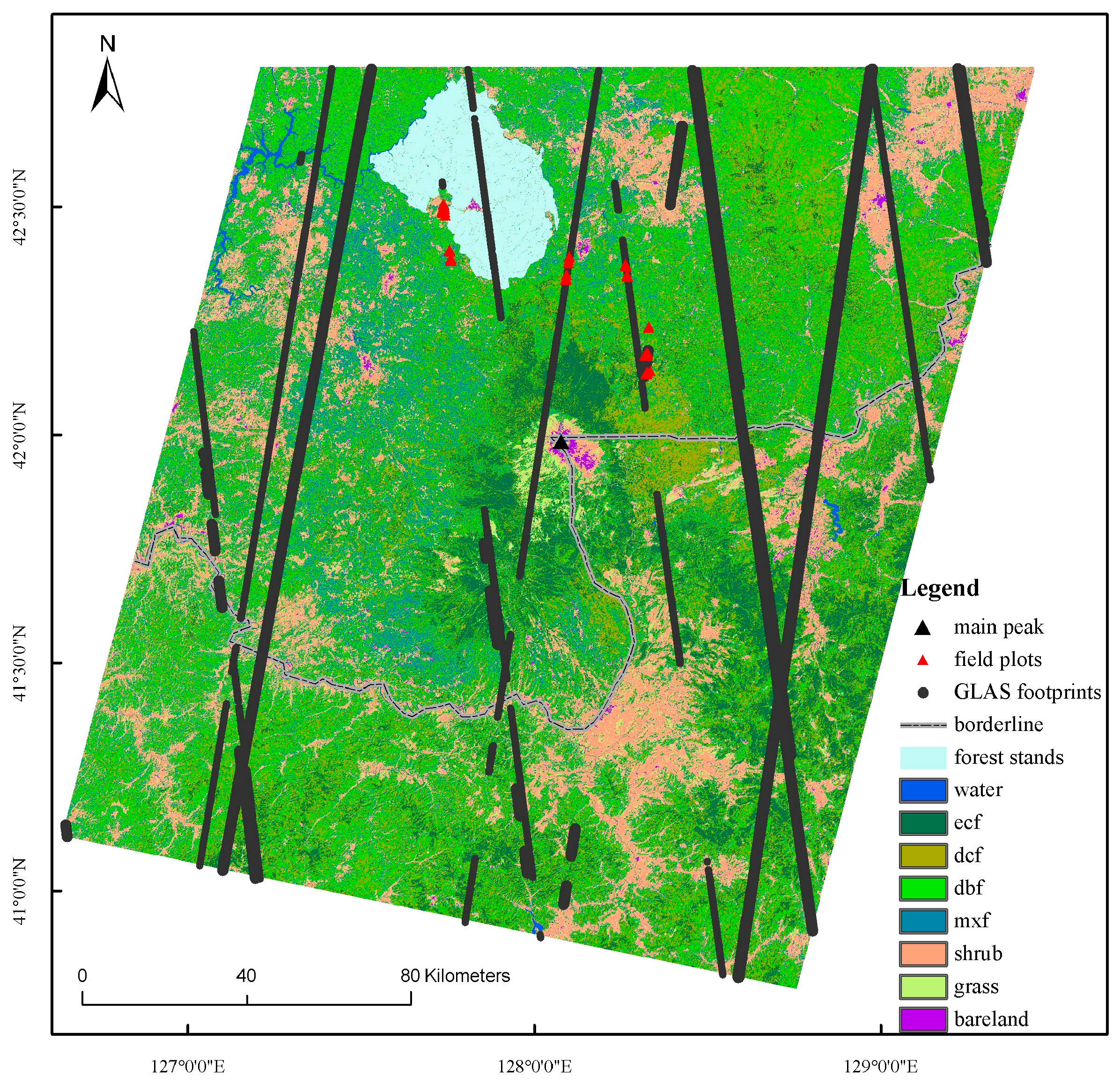
Figure 2.
LAI map.

Figure 3.
Canopy closure map.

Figure 4.
Map of AGB in the Changbai Mountain region.

Figure 5.
Distribution of forest AGB from AGB predicted map in five classes.

Figure 6.
Comparison of forest inventory AGB with GLAS- and TM-derived AGB.
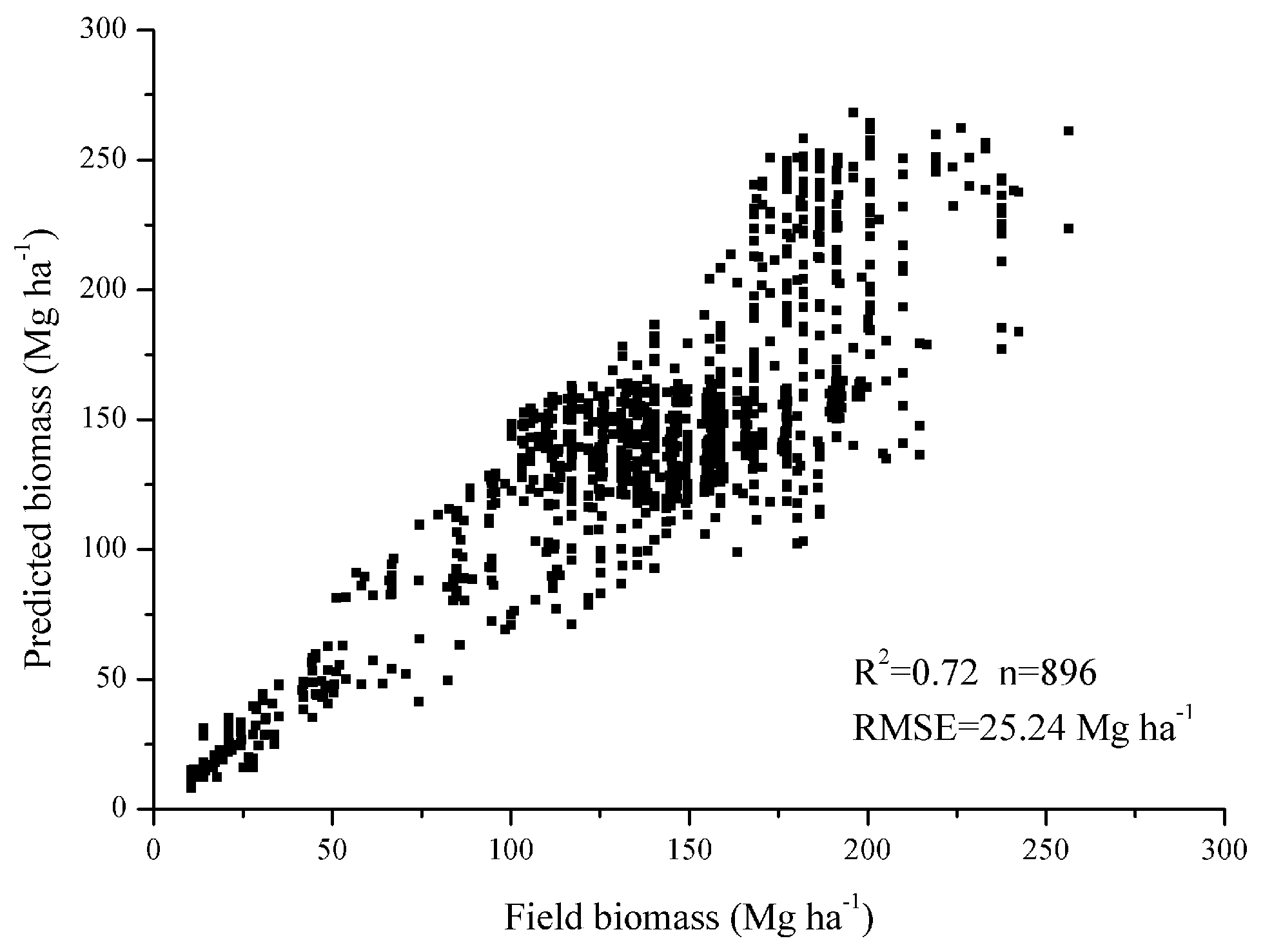
Figure 7.
Relative importance of remote sensing variables in modeling AGB of four forest types.

Figure 8.
For tree crown of a given size, canopy cover (B) is independent of canopy height, but canopy closure (A) is dependent of canopy height. In this example, B1 = B2, but A1> A2 [63].
Figure 8.
For tree crown of a given size, canopy cover (B) is independent of canopy height, but canopy closure (A) is dependent of canopy height. In this example, B1 = B2, but A1> A2 [63].
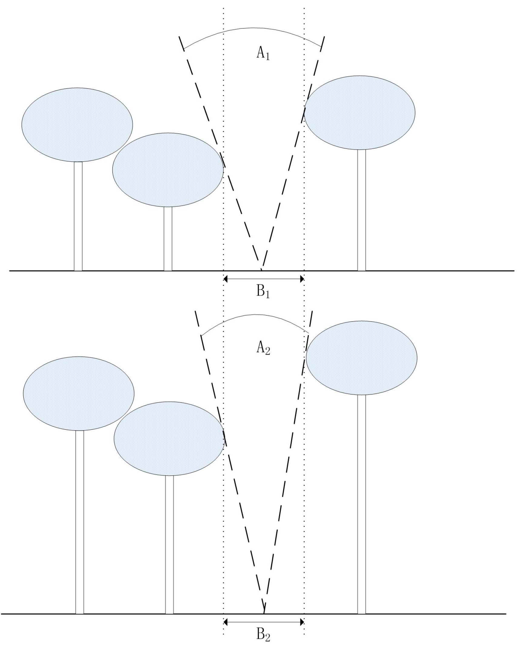

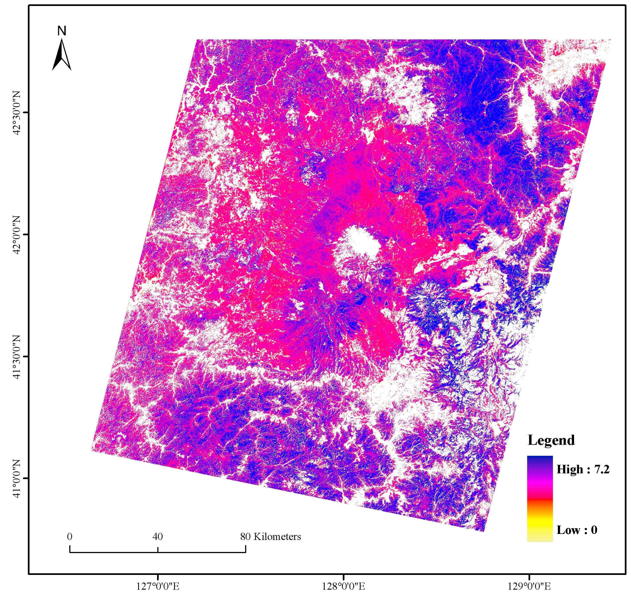
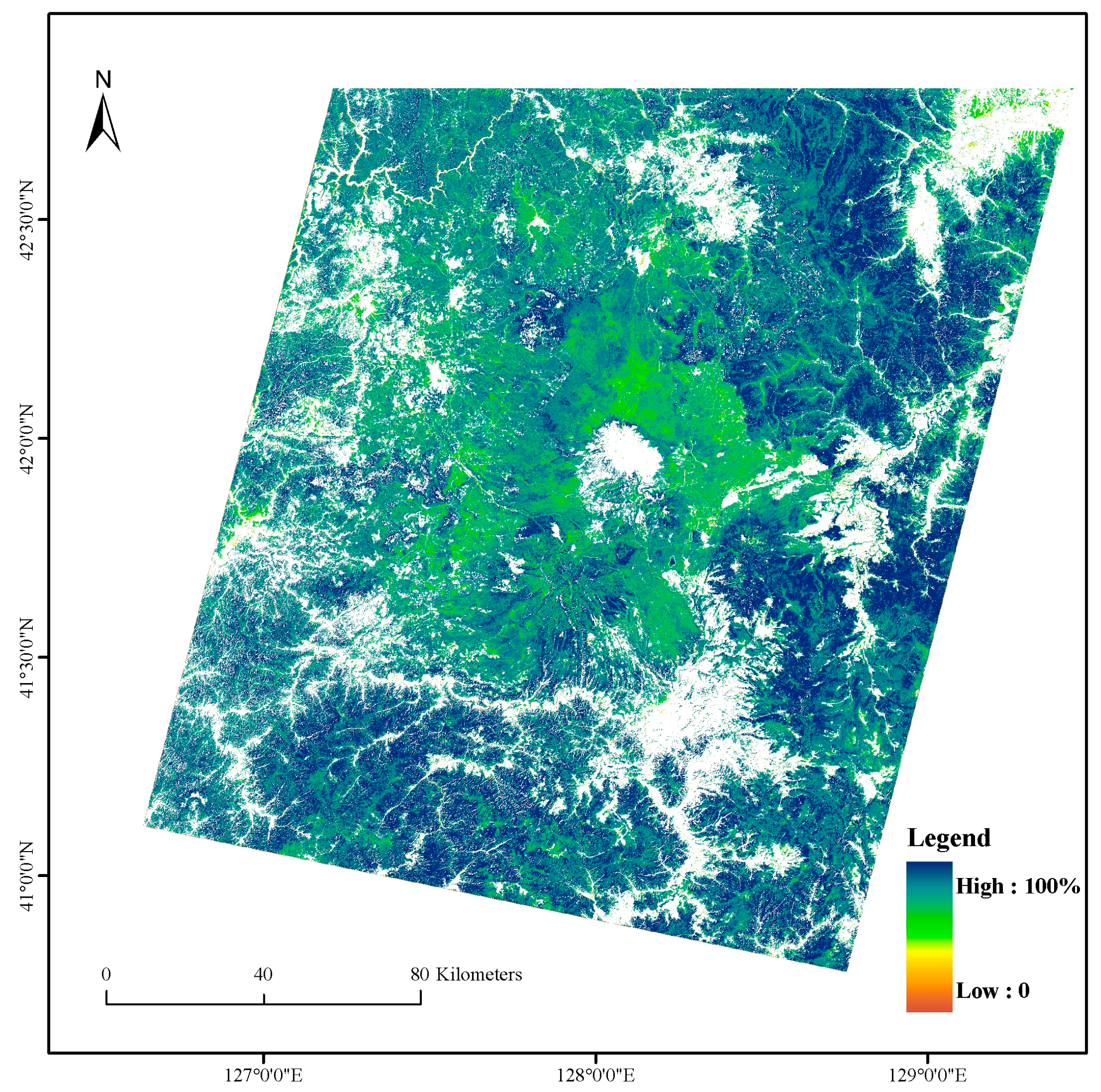
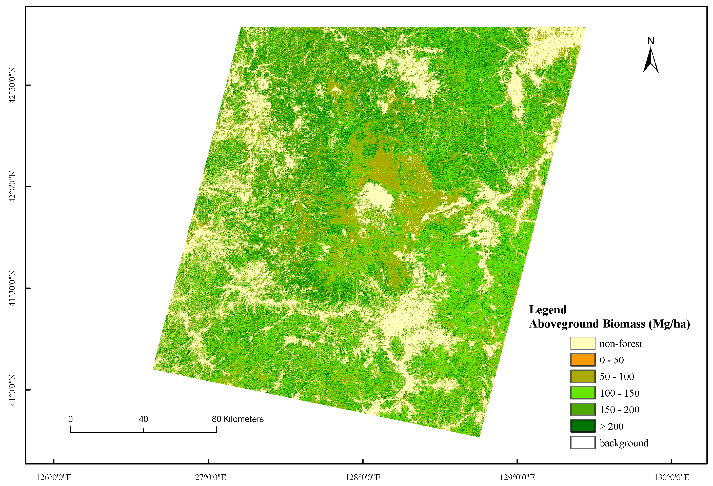
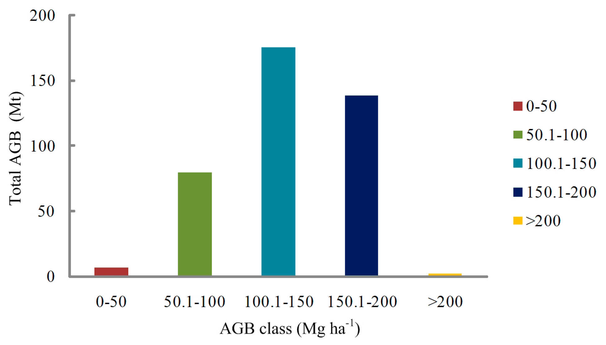
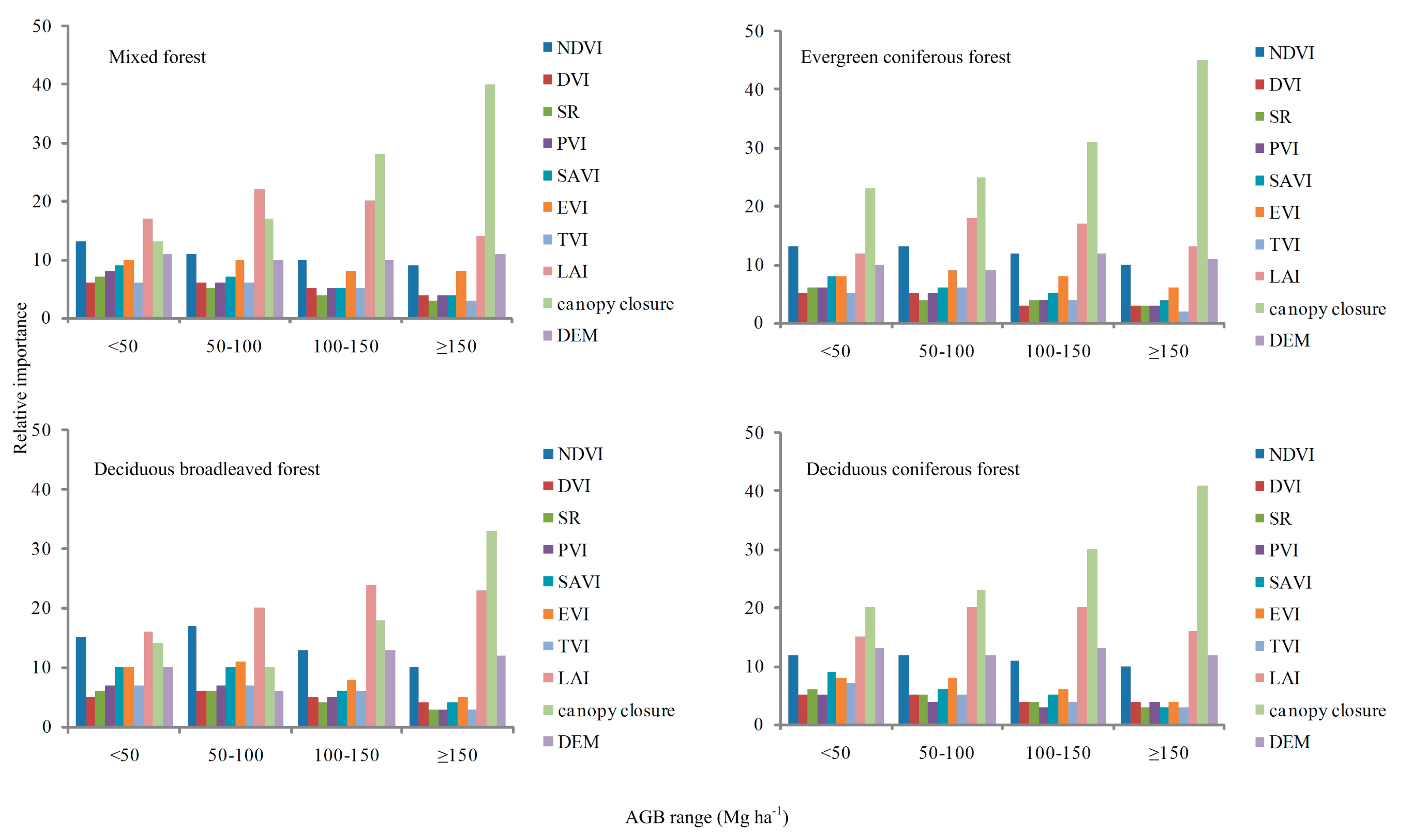
Table 1.
Summary of field data: Nt is the total number of all field forest plots; and Necf, Ndcf, Ndbf, and Nmxf are the total number of evergreen coniferous forest, deciduous coniferous forest, deciduous broadleaved forest, and mixed forest plots, respectively.
Table 1.
Summary of field data: Nt is the total number of all field forest plots; and Necf, Ndcf, Ndbf, and Nmxf are the total number of evergreen coniferous forest, deciduous coniferous forest, deciduous broadleaved forest, and mixed forest plots, respectively.
| Source | Nt | Necf | Ndcf | Ndbf | Nmxf | AGB Range (Mg·ha−1) | LAI Range |
|---|---|---|---|---|---|---|---|
| NFRI | 2911 | 756 | 571 | 762 | 822 | 10.52–303.84 | |
| field survey | 58 | 5 | 4 | 30 | 21 | 7.73–323.63 | |
| field survey | 40 | 12 | 5 | 7 | 16 | 1.73–7.49 |
Table 2.
Definition of GLAS waveform variables.
| GLAS Waveform Variables | Definition |
|---|---|
| meanh, medh | Mean and median canopy height calculated from waveform [57] |
| wflen, h14 | Waveform length and top tree height from GLA14 product |
| eratio | Vegetation to surface energy ratio from waveform as calculated by [38] |
| h10, h20, …, h100 | Decile heights for waveform energy to reach 10%, 20%, …,100% of the total energy starting from signal end [38] |
| h25, h75 | Quartile heights for waveform energy to reach 25% and 75% of the total energy starting from signal end [38] |
| lead, trail | Leading edge extent and trailing edge extent calculated from the waveform [56] |
| hslope | A terrain index calculated from a function of waveform length, footprint size, and slope [8] |
Table 3.
Parameters of the look up table in LAI estimation
| Parameter | Range | Step of Chance | No. of Simulations |
|---|---|---|---|
| Solar zenith | 0°–90° | 5° | 16 |
| View zenith | 0°–65° | 5° | 13 |
| Bands | 6 | 1 | 6 |
| Leaf area index | 0.1–8 | 0.1 | 80 |
| Canopy cover | 0–1 | 0.5 | 20 |
Table 4.
Vegetation indices derived from TM data.
| Vegetation Indices | Formula | Reference |
|---|---|---|
| NDVI | (bandNIR−bandRED)/(bandNIR + bandRED) | Tucker [78] |
| DVI | bandNIR − bandRED | Tucker [78] |
| SR | bandRED/bandNIR | Colombo et al. [74] |
| PVI | (bandNIR− a×bandRED− b)/(1 + a2)0.5 where a = 0.96916, b = 0.084726 | Richardson and Everitt [77] |
| SAVI | 1.5 × (bandNIR − bandRED)/(bandNIR + bandRED + 0.5) | Huete [75] |
| EVI | 2.5 × (bandNIR − bandRED)/(bandNIR + 6bandRED −7.5bandBLUE + 1) | Huete et al. [76] |
| TVI | 0.5 × (120(bandNIR−bandGREEN) − 200(bandRED−bandGREEN)) | Broge and Leblanc [73] |
Table 5.
LAI estimation of four forest types.
| Forest Types | LAI Range | Mean LAI |
|---|---|---|
| Evergreen coniferous forest | 1.1–7.0 | 3.8 |
| Deciduous coniferous forest | 0–6.8 | 3.6 |
| Deciduous broadleaved forest | 0–6.9 | 4.0 |
| Mixed forest | 1.2–7.2 | 3.7 |
Table 6.
Canopy closure estimation of four forest types.
| Forest Types | Canopy Closure Range (%) | Mean Canopy Closure (%) | Stand Deviation |
|---|---|---|---|
| Evergreen coniferous forest | 40.2–98.5 | 86.8 | 7.12 |
| Deciduous coniferous forest | 27.1–99.1 | 88.3 | 9.85 |
| Deciduous broadleaved forest | 25.0–99.5 | 89.2 | 10.24 |
| Mixed forest | 32.6–98.7 | 86.5 | 9.06 |
Table 7.
Stratified regression models of AGB estimated from GLAS waveform data. Adjusted R2 were the Goodness of Fit for four forest types (B = AGB, N = number of GLAS footprints sampled by forest plots used in each model).
Table 7.
Stratified regression models of AGB estimated from GLAS waveform data. Adjusted R2 were the Goodness of Fit for four forest types (B = AGB, N = number of GLAS footprints sampled by forest plots used in each model).
| Forest Types | Model | R2-a | N |
|---|---|---|---|
| Evergreen coniferous forest | ln(B) = 0.5128 meanh+ 0.0918trail − 0.7033h25 + 0.8597h50 + 0.3184h100 + 4.0624 (slope <10°) | 0.804 | 327 |
| ln(B) = 0.6243 medh + 0.2471 lead − 0.1918 trail − 0.7836 h25 +1.0716 h50 + 0.3441 h100 + 4.8015 (slope ≥10°) | 0.787 | 184 | |
| Deciduous coniferous forest | ln(B) = 0.2778 wflen + 0.1034trail−0.3609 h50 + 0.5466 h75 + 0.2989 h100 + 4.1116 (slope <10°) | 0.813 | 234 |
| ln(B) = 0.5846 h14 + 0.2613 lead −0.2089trail−1.0773 h50 + 0.2122 h75 + 0.2989 h100 + 4.0624 (slope ≥10°) | 0.786 | 116 | |
| Deciduous broadleaved forest | ln(B) = 0.3358 lead + 0.3749 h75 + 0.1516 h100 − 0.0889 eratio− 0.3196 h20− 1.4819 ln(h25) + 6.8414 (slope <10°) | 0.793 | 472 |
| ln(B) = 0.8283 lead − 0.3189 trail + 0.1668 h75 + 0.3292 h100 − 0.1173 eratio− 0.3724 h40 − 0.8618 ln(h50) + 0.2159 hslope+ 3.0177 (slope ≥10°) | 0.772 | 163 | |
| Mixed forest | ln(B) = 0.5735 h75 − 0.2833eratio − 0.1981 h25 + 0.2264 h100 + 3.6923 (slope <10°) | 0.798 | 355 |
| ln(B) = 0.4763lead − 0.1587trail − 0.1007h25 + 0.0819h100 + 0.6691 hslope + 3.4732 (slope ≥10°) | 0.765 | 128 |
Table 8.
AGB predicted from GLAS data on slopes <10° and ≥10° were compared with AGB converted from forest inventory data for four forest types. R2 and RMSE (in parentheses) values correspond to each forest type.
Table 8.
AGB predicted from GLAS data on slopes <10° and ≥10° were compared with AGB converted from forest inventory data for four forest types. R2 and RMSE (in parentheses) values correspond to each forest type.
| Forest Types | R2 and RMSE (Mg·ha−1) in AGB Model Validation | |
|---|---|---|
| <10° | ≥10° | |
| Evergreen coniferous forest | 0.811(9.85) | 0.796(13.97) |
| Deciduous coniferous forest | 0.825(10.34) | 0.825(10.34) |
| Deciduous broadleaved forest | 0.829(12.29) | 0.807(17.93) |
| Mixed forest | 0.878(11.40) | 0.823(18.62) |
© 2017 by the authors. Licensee MDPI, Basel, Switzerland. This article is an open access article distributed under the terms and conditions of the Creative Commons Attribution (CC BY) license (http://creativecommons.org/licenses/by/4.0/).
Share and Cite
MDPI and ACS Style
Chi, H.; Sun, G.; Huang, J.; Li, R.; Ren, X.; Ni, W.; Fu, A. Estimation of Forest Aboveground Biomass in Changbai Mountain Region Using ICESat/GLAS and Landsat/TM Data. Remote Sens. 2017, 9, 707. https://doi.org/10.3390/rs9070707
AMA Style
Chi H, Sun G, Huang J, Li R, Ren X, Ni W, Fu A. Estimation of Forest Aboveground Biomass in Changbai Mountain Region Using ICESat/GLAS and Landsat/TM Data. Remote Sensing. 2017; 9(7):707. https://doi.org/10.3390/rs9070707
Chicago/Turabian StyleChi, Hong, Guoqing Sun, Jinliang Huang, Rendong Li, Xianyou Ren, Wenjian Ni, and Anmin Fu. 2017. "Estimation of Forest Aboveground Biomass in Changbai Mountain Region Using ICESat/GLAS and Landsat/TM Data" Remote Sensing 9, no. 7: 707. https://doi.org/10.3390/rs9070707
Note that from the first issue of 2016, this journal uses article numbers instead of page numbers. See further details here.