Estimation of Winter Wheat Above-Ground Biomass Using Unmanned Aerial Vehicle-Based Snapshot Hyperspectral Sensor and Crop Height Improved Models

Abstract

Correct estimation of above-ground biomass (AGB) is necessary for accurate crop growth monitoring and yield prediction. We estimated AGB based on images obtained with a snapshot hyperspectral sensor (UHD 185 firefly, Cubert GmbH, Ulm, Baden-Württemberg, Germany) mounted on an unmanned aerial vehicle (UAV). The UHD 185 images were used to calculate the crop height and hyperspectral reflectance of winter wheat canopies from hyperspectral and panchromatic images. We constructed several single-parameter models for AGB estimation based on spectral parameters, such as specific bands, spectral indices (e.g., Ratio Vegetation Index (RVI), NDVI, Greenness Index (GI) and Wide Dynamic Range VI (WDRVI)) and crop height and several models combined with spectral parameters and crop height. Comparison with experimental results indicated that incorporating crop height into the models improved the accuracy of AGB estimations (the average AGB is 6.45 t/ha). The estimation accuracy of single-parameter models was low (crop height only: R² = 0.50, RMSE = 1.62 t/ha, MAE = 1.24 t/ha; R₆₇₀ only: R² = 0.54, RMSE = 1.55 t/ha, MAE = 1.23 t/ha; NDVI only: R² = 0.37, RMSE = 1.81 t/ha, MAE = 1.47 t/ha; partial least squares regression R² = 0.53, RMSE = 1.69, MAE = 1.20), but accuracy increased when crop height and spectral parameters were combined (partial least squares regression modeling: R² = 0.78, RMSE = 1.08 t/ha, MAE = 0.83 t/ha; verification: R² = 0.74, RMSE = 1.20 t/ha, MAE = 0.96 t/ha). Our results suggest that crop height determined from the new UAV-based snapshot hyperspectral sensor can improve AGB estimation and is advantageous for mapping applications. This new method can be used to guide agricultural management.

1. Introduction

Above-ground biomass (AGB) [1] reflects the status of crop growth and is related to solar energy utilization, yield and grain quality [2,3]. Therefore, AGB is considered one of the most important biochemical crop parameters [4,5,6], and correct estimation of AGB can help improve crop monitoring and yield prediction [7]. Estimation of AGB is also important for ecological research at regional and global scales [8] and has been employed in global carbon cycle [9,10,11] and climate change [12,13,14] studies.

Manual methods for measuring AGB are time consuming and destructive. Prior to the emergence of remote sensing technology, large AGB surveys were limited by labor and resources [4,5,6]. Hyperspectral technology has shown great potential for monitoring of crop parameters [15,16]. Hyperspectral sensors can obtain spectral features based on radiation from visible to near-infrared wavelengths, and advancements in technology have increased the number of features that can be collected [17,18,19]. Spectral features and indices are important variables for estimating hyperspectral crop parameters [20,21,22,23,24,25,26], and many studies have estimated AGB using a combination of narrow spectral bands and vegetation indices [27,28,29].

The development and application of unmanned aerial vehicles (UAVs) as remote sensing platforms [15,30,31,32] have increased rapidly over the past decade. Additionally, UAVs can obtain remote sensing images with higher temporal, spatial and ground resolution than satellites. Small-sized remote sensing sensors can be mounted on UAVs, making UAV platforms increasingly popular in agricultural applications [15,31]. Use of UAVs in agricultural and environmental applications has numerous advantages compared with conventional aerial vehicles, including lower cost, weight, flight speed and flight altitude [15].

Previous studies have proposed various methods and sensors for agricultural monitoring based on UAV remote sensing. The results of Ribeiro et al. [33] (geometric products), Bendig et al. [34,35] (plant height, biomass) and Jannoura et al. [36] (LAI) indicated that digital cameras with visible and infrared spectra are efficient and flexible for monitoring agricultural crop parameters. Berni et al. [37] suggested that thermal infrared cameras mounted on UAVs show potential for environmental and agricultural applications (mapping canopy conductance and crop water stress). The results of Vonbueren et al. [38], Vega et al. [39] and Honkavaara et al. [40] indicated that data from UAV-based spectral cameras can be used to monitor parameters (e.g., crop height, yield, aboveground biomass and nitrogen content) of various plants, such as grass, wheat and sunflowers. However, the use of UAVs for agricultural monitoring is limited by the weight of hyperspectral imaging systems, the complexity of image processing and the cost of sensors [41,42].

Many powerful techniques/methods had been employed by previous researchers to make full use of the hyperspectral information, such as partial least squares regression (PLSR), support vector machine regression (SVR), artificial neural network (ANN) and random forest regression (RF). The results of Jin et al. [25] (leaf water content), Fu et al. [43] (biomass) and Nguyen et al. [44] (rice leaf growth and nitrogen status) indicated that PLSR is efficient and flexible for hyperspectral monitoring of agricultural crop parameters. Yang et al. [45] (LAI) and Atzberger et al. [46] (LAI, leaf chlorophyll content, equivalent leaf water thickness) suggested that ANN has great potential for biophysical canopy variables’ estimation. Yang et al. [47] suggested that SVM shows great potential for rice leaf area index estimation. Han et al. [48] suggested that RF is more efficient than SVM in apple tree canopy LAI estimation. The results of Yuan et al. [49] indicated that RF can be used to monitor the soybean leaf area index over the whole growth period.

The objective of this study was to evaluate the performance of AGB estimations based on hyperspectral data (canopy surface information) and crop height (vertical information about crop growth). A snapshot hyperspectral sensor mounted on a UAV was used to obtain hyperspectral and high-resolution panchromatic images. Using image fusion and photogrammetry, we obtained the canopy hyperspectral reflectance and crop height of winter wheat. Hyperspectral data and crop height were used to construct AGB estimation models, and model accuracy was validated with field data.

2. Materials and Methods

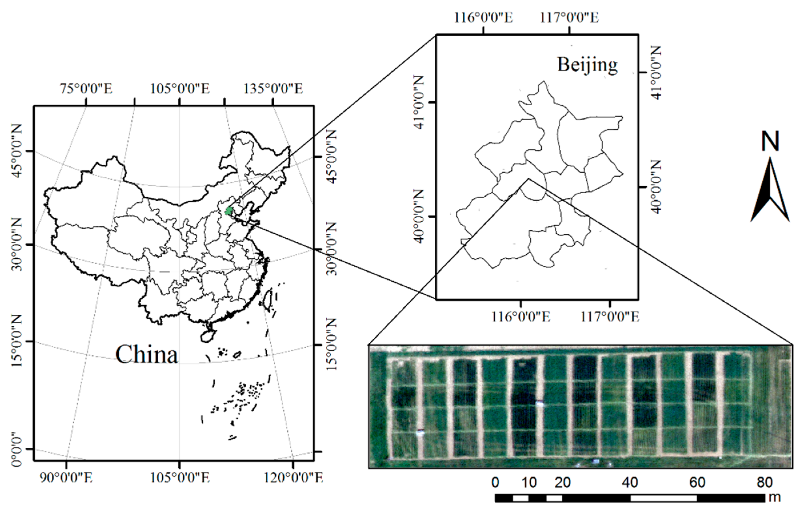
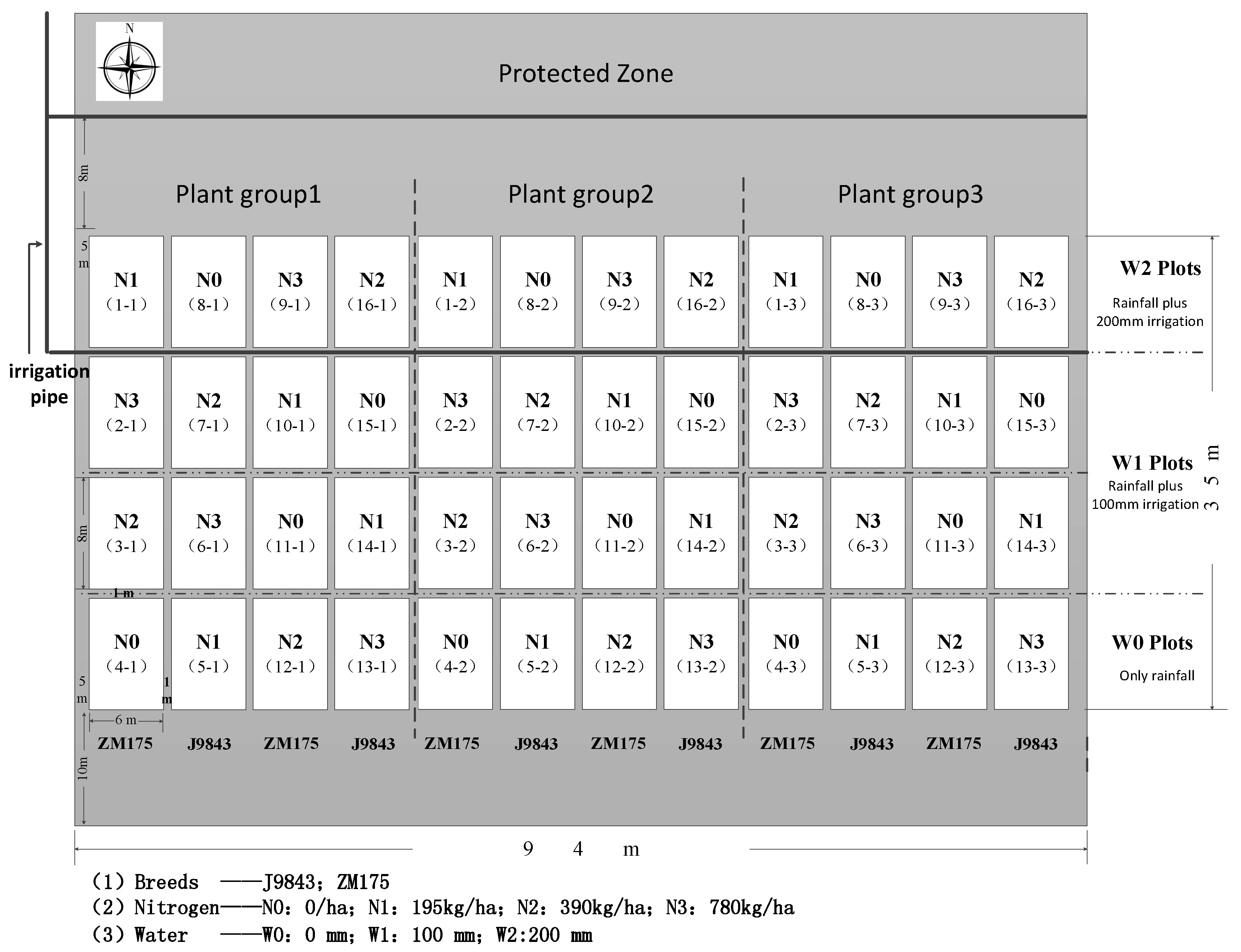
Winter wheat was grown on 48 plots with different amounts of nitrogen fertilizer and irrigation levels. We measured spectral features of the crops and analyzed the relationships between crop height, UHD 185 (UHD 185 firefly, Cubert GmbH, Ulm, Baden-Württemberg, Germany) spectrometer hyperspectral data, ASD Field Spec 3 spectrometer hyperspectral data and winter wheat AGB.

2.1. Study Area

Experiments were conducted at the Xiao Tangshan National Precision Agriculture Research Center of China, which has an area of ~2 square kilometers and is located in Changping District (115°50′17″～116°29′49″E, 40°2′18″～40°23′13″N) of Beijing City, China (Figure 1). Changping District has an average altitude of 36 m, a warm temperate semi-humid continental monsoon climate, average rainfall of 450 mm, average low temperature of −10 °C–7.5 °C and an average high temperature of 35 °C–40 °C. Meteorological data were acquired from the China Meteorological Data Service [50].

2.2. Data

2.2.1. AGB and Crop Height Measurement

The sampling plan is shown in Figure 2. Crops were divided into three groups, and each group included a total of 16 winter wheat samples. Samples received different levels of irrigation and nitrogen fertilizer. The irrigation levels included rainfall only (W0), rainfall plus the normal irrigation level (W1, 100 mm) and rainfall plus twice the normal irrigation level (W2, 200 mm). The nitrogen fertilizer levels included no fertilizer (N0), one-half the normal fertilization level (N1, 195 kg/ha), the normal fertilization level (N2, 390 kg/ha) and twice the normal fertilization level (N3, 780 kg/ha).

During sampling, 20 stems were collected near the center of each plot. Crop height was measured using a straightedge. Samples were taken to the laboratory for processing and stored in paper bags. Leaves and stems were dried at 80 °C to remove moisture. Until the samples became constant weight (about 24 h), the dry weight of each sample was recorded. Winter wheat AGB was calculated using Equation (1)

$$\mathrm{AGB}=\frac{m\times n}{20\times l}$$

where m is the dry weight of the sample, n is the number of winter wheat ears per unit area and l is the row spacing.

2.2.2. Snapshot Hyperspectral Sensor

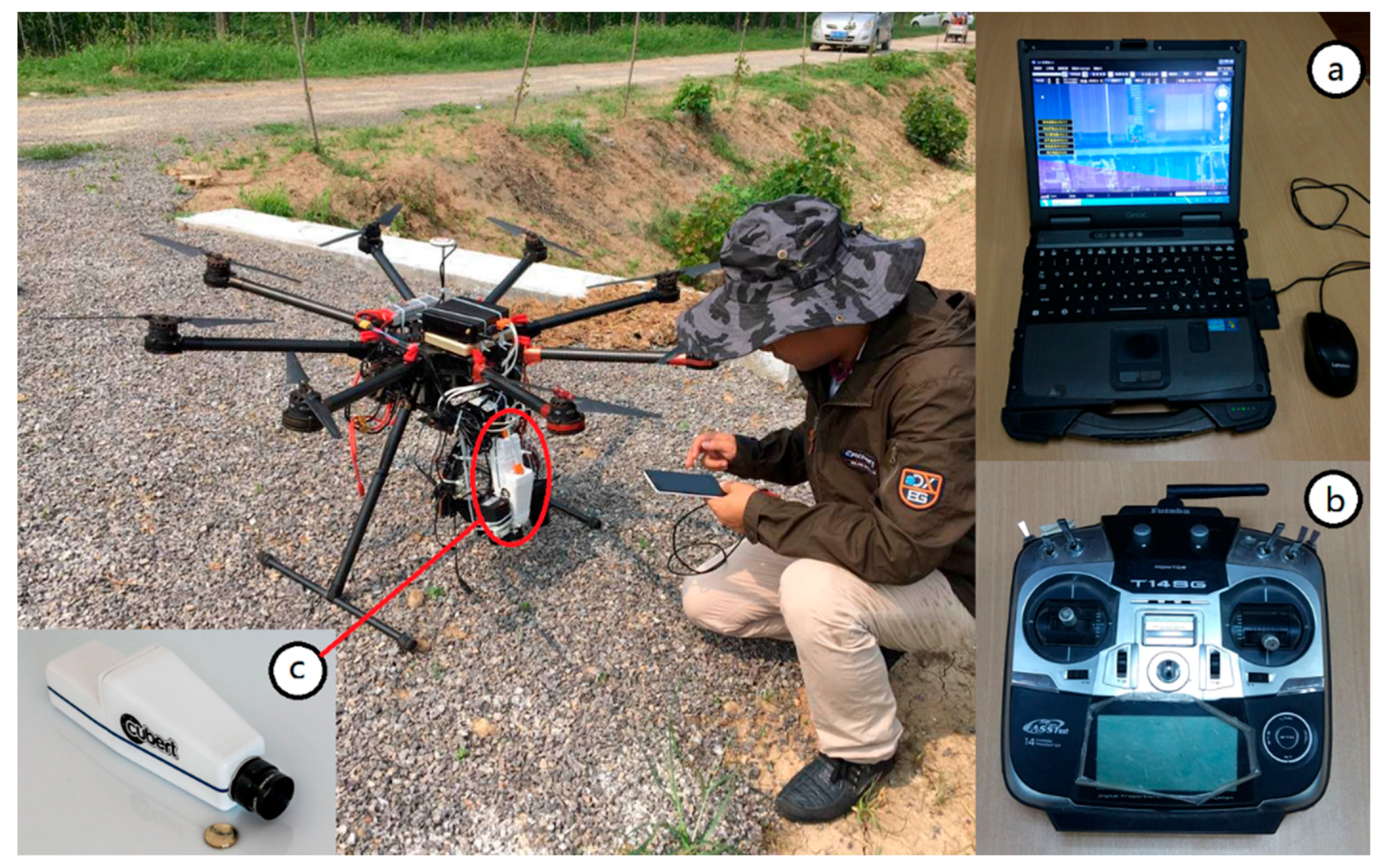
The UHD 185 Firefly (UHD 185) is a new type of snapshot hyperspectral sensor, characterized by short exposure and integration time. The sensor weighs 0.47 kg, and its dimensions are 195 × 67 × 60 mm. It can obtain reflected radiation from the visible to near-infrared spectra. The sensor can capture 450–950-nm wavelengths, while maintaining a reasonable balance of image and good spectral resolution (4 nm). Radiation is recorded and processed as a 1000 × 1000 (1 band) panchromatic image and a 50 × 50 (125 bands) hyperspectral image. The acquired panchromatic images are rich in texture information, and stitching is relatively simple; however, images lack spectral information. The 50 × 50 (125 bands) hyperspectral images are characterized by rich spectral information, but lack texture information. Hyperspectral image fusion [19] was used to splice the UHD 185 hyperspectral image. After fusion, all images were stitched together using an image stitching process.

2.2.3. Platform

The UAV UHD 185 hyperspectral system was designed by the National Engineering Research Center for Information Technology in Agriculture (NERCITA) of China [51]. The system was composed of three parts, including a ground control system, UAV and UHD 185 hyperspectral system and post-processing software. As shown in Figure 3, the ground control system included a DJI S1000 UAV (SZ DJI Technology Co., Ltd., Sham Chun, Guangdong Province, China) [52] (Figure 3), the DJI ground-control station (software, Figure 3a), reinforcement notebook computer (hardware, Figure 3a) and remote controller (Figure 3b). The UHD 185 hyperspectral system consisted of a cloud platform and the UHD 185 hyperspectral sensor (Figure 3c). The post-processing software consisted of software for stitching, as well as radiation and geometry correction (e.g., as Cubert [19], Agisoft PhotoScan [53] and ENVI 5.1 [54]).

The DJI S1000 UAV is a UAV platform with eight propellers and a multirotor, which improve stability at slow flight speeds and low altitude. When equipped with two 18,000-mAh (25 V) batteries, the UAV can run for 30 min with a take-off weight of 6 kg, flying altitude of 50 m and flight speed of 8 m/s. Flights were conducted during the flagging (26 April 2015) and flowering (13 May 2015) stages of winter wheat with ground winter wheat ASD measurement. Each flight covered a field area of 6000 square meters and lasted ~20 min. Remote sensing images acquired from high-altitude platforms typically require atmospheric correction; conversely, the UHD 185 images were obtained under stable light conditions in this study, and atmospheric correction was not required. We compared hyperspectral data acquired with the UHD 185 and ground ASD.

2.2.4. ASD Measurement

Ground winter wheat canopy reflectance was measured using an ASD Field Spec 3 spectrometer (Analytical Spectral Devices, Boulder, Colorado, CO, USA; abbreviated as ASD). Measurements were collected during the flagging (26 April 2015) and flowering (13 May 2015) stages of winter wheat growth. After the UAV flight (from 11 a.m.–2 p.m.), ground measurements were carried out under windless conditions and stable light levels. Winter wheat canopy reflectance was measured 10 times at the center of each plot, and the average reflectance was recorded. The reflectance obtained by ground-based ASD and UAV-mounted UHD spectrometers was compared.

2.3. Methods

After the UHD 185 images were stitched together, a ground resolution of 1 cm was obtained for the hyperspectral images. We used ENVI ROI (ENVI image processing and analysis software, from ITT Visual Information Solutions, Boulder, CO, USA) tools to calculate the average canopy spectral reflectance of each plot and selected bands of 462 nm–882 nm to avoid unstable spectra; this band range should also be selected for this study to obtain the best combination of spectral bands and indices. The first two groups of crops were used to build the AGB models, and the remaining group was used as the validation set. With two UAV flights and ground measurements, we have 64 sets of data for AGB model building and 32 sets of data for AGB model validating.

2.3.1. Selection of Spectral Bands and Indices

To construct linear AGB estimation models, five spectral specific bands and fourteen spectral vegetation indices were selected from the literature [55,56,57,58,59,60,61,62], including: B₄₇₀, G₅₅₀, R₆₇₀, R₆₈₀, Nir₇₅₀, Nir₈₀₀, the Ratio Vegetation Index (RVI) [55], the Normalized Difference Vegetation Index (NDVI) [20], Enhanced VI (EVI) [56], Two-band Enhanced VI (EVI2) [57], the Greenness Index (GI) [58], the Modified Soil-Adjusted Vegetation Index (MSAVI) [59], the Optimized Soil Adjusted Vegetation Index (OSAVI) [60], Wide Dynamic Range VI (WDRVI) [26], Triangular VI (TVI) [61,62], Difference Vegetation Index (DVI1, DVI2, DVI3) [55], Modified Triangular VI (MTVI1) [61] and Modified Triangular VI (MTVI2) [61] (

Table 1. Specific bands and Spectral vegetation indices. Ratio Vegetation Index (RVI) [55], the Normalized Difference Vegetation Index (NDVI) [20], Enhanced VI (EVI) [56], Two-band Enhanced VI (EVI2) [57], the Greenness Index (GI) [58], the Modified Soil-Adjusted Vegetation Index (MSAVI) [59], the Optimized Soil Adjusted Vegetation Index (OSAVI) [60], Wide Dynamic Range VI (WDRVI) [26], Triangular VI (TVI) [61,62], Difference Vegetation Index (DVI1, DVI2, DVI3) [55], Modified Triangular VI (MTVI1) [61] and Modified Triangular VI (MTVI2).

Spectral Indices	Characteristics and Functions	Definition	Reference
B470	Reflectance of 470 nm	R470	[55]
G550	Reflectance of 550 nm	R550	[55]
R670	Reflectance of 670 nm	R670	[55]
R680	Reflectance of 680 nm	R680	[55]
Nir800	Reflectance of 800 nm	R800	[55]
RVI	Ratio of near infrared and red bands	R800/R680	[55]
NDVI	Responds to change in the amount of green biomass and more efficiently in vegetation with low to moderate density	$\frac{R_{800}-R_{680}}{R_{800}+R_{680}}$	[20]
EVI	Estimate vegetation LAI, biomass and water content, and improve sensitivity in high-biomass regions	$\frac{2.5\left(R_{800}-R_{680}\right)}{R_{800}+6R_{680}-7.5R_{550}+1}$	[56]
EVI2	Similar to EVI, but without blue band and good for atmospherically corrected data	$\frac{2.5\left(R_{800}-R_{680}\right)}{R_{800}+2.4R_{680}+1}$	[57]
GI	Estimate biochemical constituents and LAI at leaf and canopy levels	R550/R680	[58]
MSAVI	A more sensitive indicator of vegetation amount than SAVI at canopy level	0.5[2R800 + 1 − ((2R800 + 1)2 − 8(R800 − R670))1/2]	[59]
OSAVI	Similar to MSAVI, but more applicable in agricultural applications, whereas MSAVI is recommended for more general purposes	$\frac{1.16\left(R_{800}-R_{670}\right)}{R_{800}+R_{670}+0.16}$	[60]
WDRVI	Estimate LAI, vegetation cover, biomass; better than NDVI	$\frac{0.1R_{800}-R_{680}}{0.1R_{800}+R_{680}}$	[26]
TVI	Characterize the radiant energy absorbed by leaf pigments (Chls); note that the increase of Chls concentration also results in the decrease of the green reflectance	0.5[120(R750 − R550) − 200(R670 − R 550)]	[61,62]
DVI1	Reflectance differ of 800 nm and 680 nm	R800 − R680	[55]
DVI2	Reflectance differ of 750 nm and 680 nm	R750 − R680	[55]
DVI3	Reflectance differ of 550 nm and 680 nm	R550 − R680	[55]
MTVI1	More suitable for LAI estimation than TVI	1.2[1.2(R800 − R550) − 2.5(R670 − R550)]	[61]
MTVI2	Preserves sensitivity to LAI and resistance to Chl influence	{1.5[1.2(R800 − R550) − 2.5(R670 − R550)]}/ {(2R800 + 1)2 − [6R800− 5(R670) 1/2] − 0.5}1/2	[61]

Note: UHD 185 data did not include bands centered in 680 or 800 because its spectral resolution was 4 nm. Therefore, UHD b680 and b800 were calculated as the average UHD reflectance at 682 and 678 nm and at 802 and 798 nm (written as Band 600 and Band 800 in the following passage), respectively.

).

2.3.2. Winter Wheat Height

It was impossible to set up stable ground elevation control points in the field due to the irrigation system used at our experimental site. Therefore, we calculated the relative crop height using digital elevation model (DEM) and digital surface model (DSM). DEM and DSM are two types of surface simulations used in surveying. A DEM conveys ground surface elevation, and a DSM is the sum of the DEM and vegetation surface. Thus, crop height can be obtained by subtracting the DEM from the DSM (Figure 4 and Equation (2)).

$$Heigh{t}_{\mathrm{crop}}=H{\mathrm{eight}}_{DSM}-Heigh{t}_{DEM}$$

In this paper, the DSM was obtained using photogrammetric technology software (Agisoft PhotoScan, Agisoft, St. Petersburg, Russia), panchromatic images and the positioning and orientation system (POS) information, all acquired by the UAV. Some soil points’ coordinate information was recorded using ARCGIS software (ARCGIS, Environmental Systems Research Institute, Inc., Redlands, CA, USA), then using ARCGIS extract tools to obtain all soil points’ elevation. The DEM was obtained by interpolating the surface elevation using ARCGIS kriging tools. After DEM and DSM were calculated, we use ARCGIS raster calculator tools to calculate the crop height map. After the above calculation, the soil part in the crop height map is about 0 m (black area in Figure 4), and the crop zone will show the crop height value (gray area in Figure 4).

2.3.3. Partial Least Squares Regression

Partial least squares regression is a statistical method introduced by Herman Wold [63] in the 1960s as an economic technique. PLSR provides an efficient way to make full use of the hyperspectral information and was also widely used in remote sensing for vegetation studying. Previous studies [64,65] indicated that PLSR has excellent capability in making use of the full spectral information. In this paper, we employed the partial least squares regression using MATLAB (MATLAB 2014a, MathWorks, Inc., Natick, MA, USA) software on Microsoft Windows.

2.3.4. Precision Evaluation

Spectral data collected from two plan groups were used for model construction, and data collected from the third group were used for validation. We used the coefficient of determination (R²), root mean square error (RMSE) and mean absolute error (MAE) to evaluate the performance of each model. Higher R² values correspond to smaller RMSE and MAE values and higher model precision. Equations (3)–(5) were used to calculate R², RMSE and MAE.

$$R^2=\frac{{{\displaystyle \sum }}_{i=1}^n{(x_i-\overline{x})}^2{(y_i-\overline{y})}^2}{{{\displaystyle \sum }}_{i=1}^n{(x_i-\overline{x})}^2{{\displaystyle \sum }}_{i=1}^n{(y_i-\overline{y})}^2}$$

$$\mathrm{RMSE}=\sqrt{\frac{{\displaystyle {\displaystyle \sum }_{i=1}^n}{(x_{\mathrm{i}}-y_i)}^2}{n}}$$

$$\mathrm{MAE}=\frac{{\displaystyle {\displaystyle \sum }_{i=1}^n}\left|x_i-y_i\right|}{n}$$

where x_i and y_i are the estimated and measured values (AGB), $\overline{x}$ and $\overline{y}$ are the average estimated and measured values and n is the sample number.

3. Results

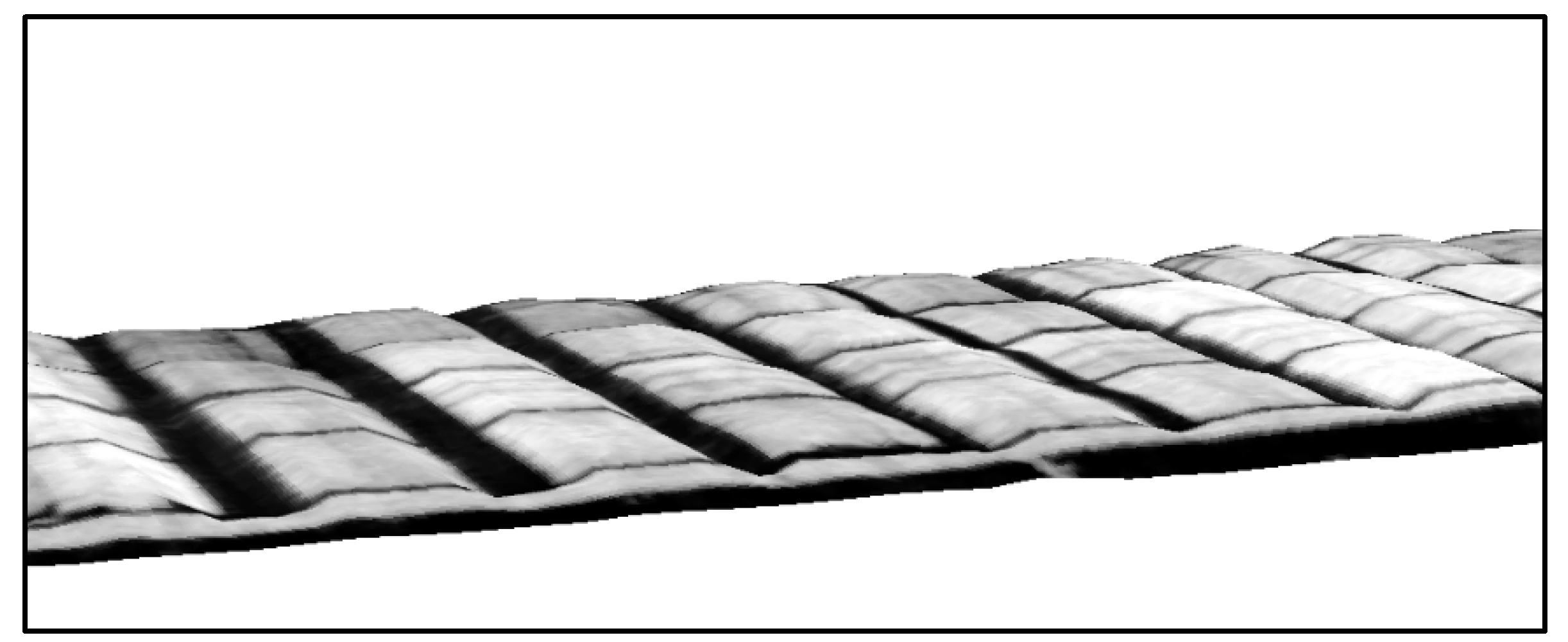
3.1. UHD Hyperspectral Data and Crop Height Analysis

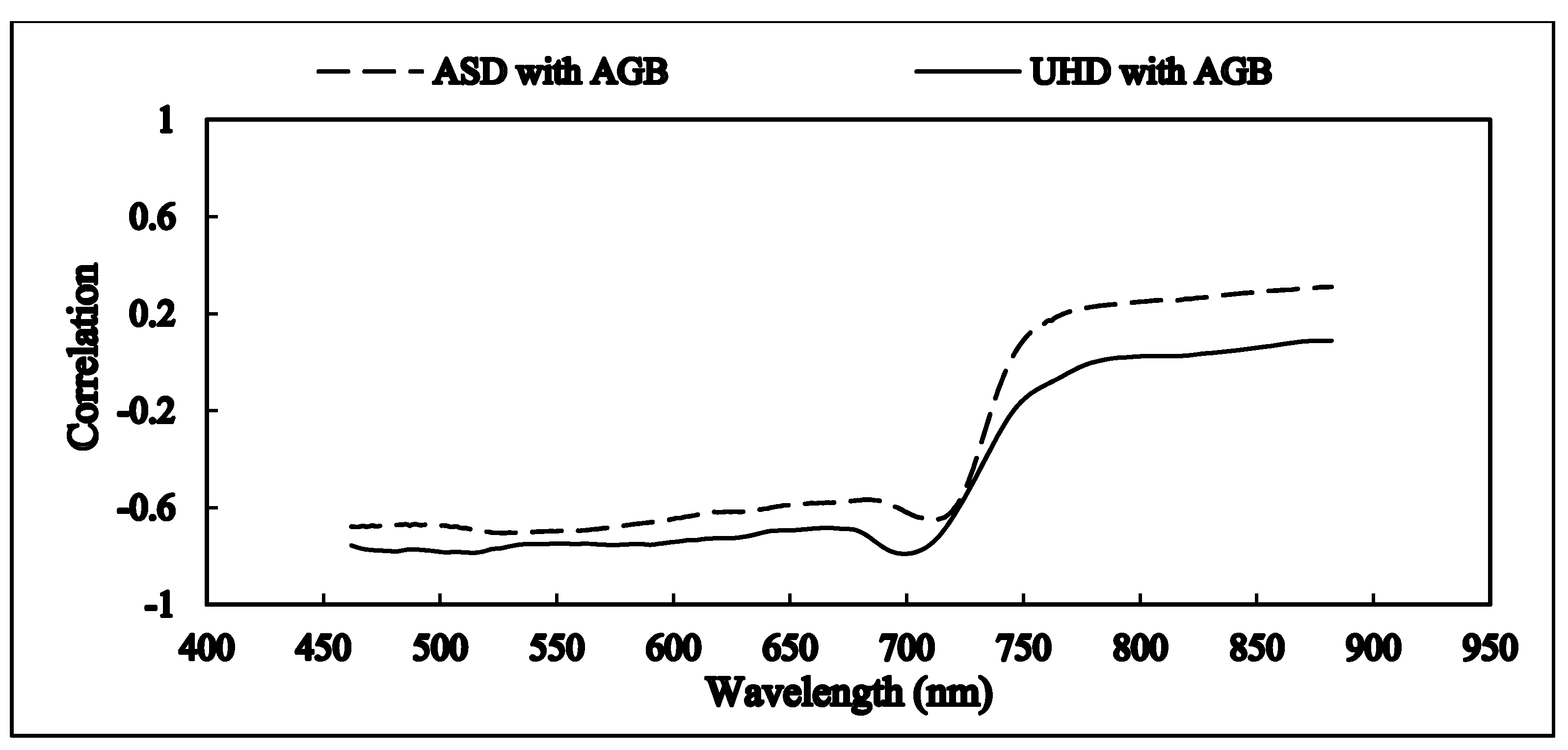
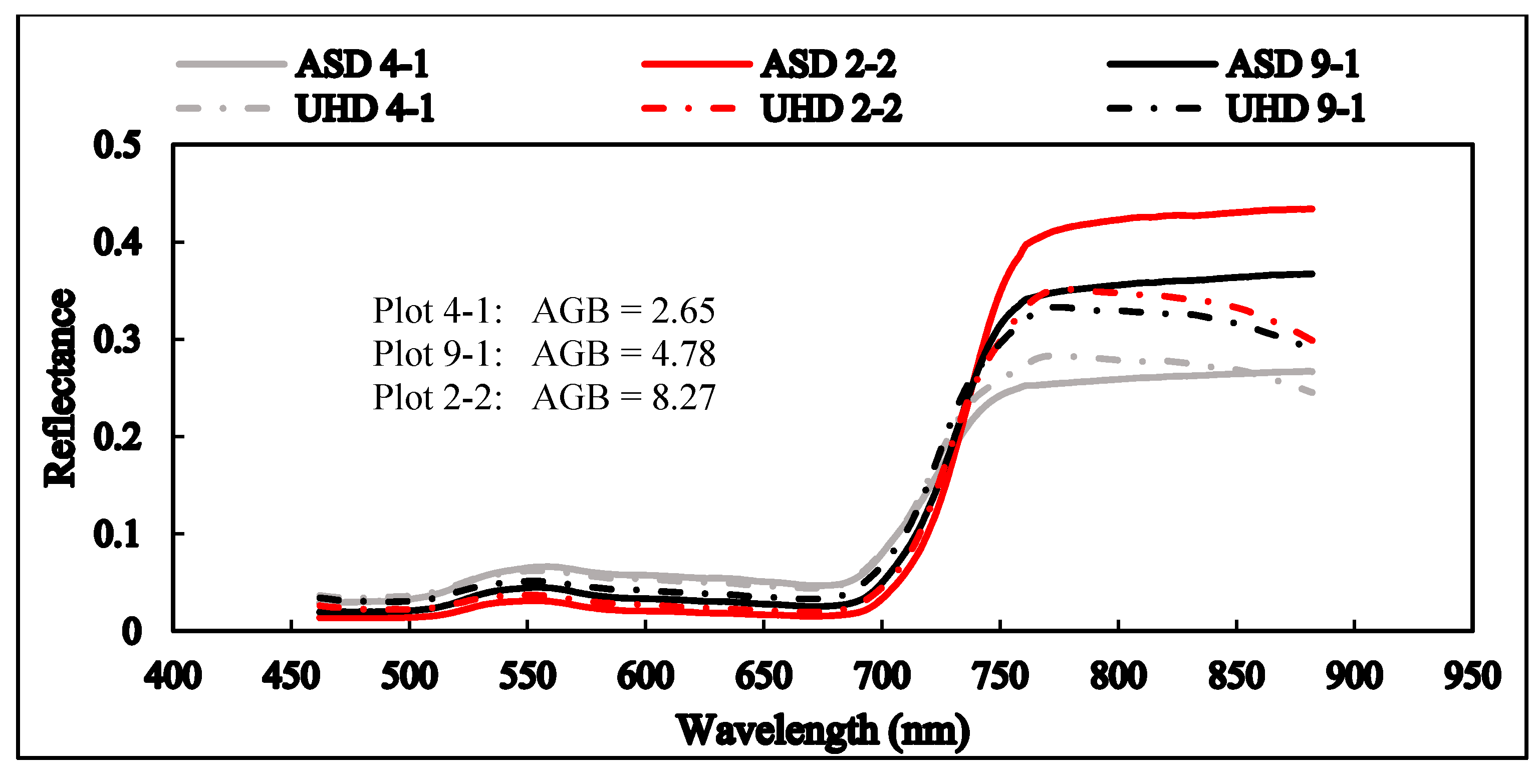
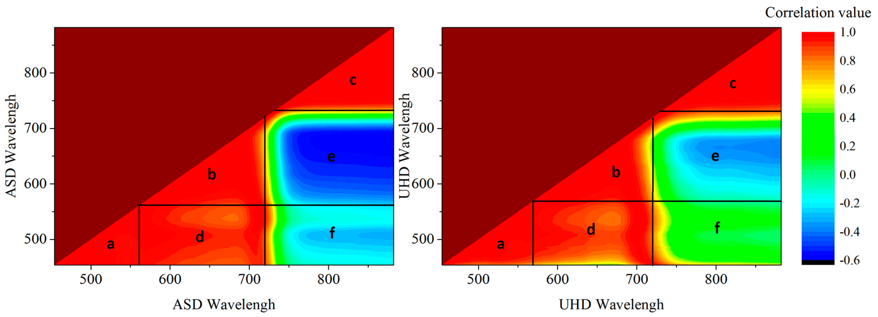
3.1.1. Analysis of ASD and UHD Hyperspectral Data

The canopy reflectance of different plots (Plots 2-2, 4-1, 9-1) is shown in Figure 5. For wavelengths in the range of 462–882 nm, typical vegetation spectral features are shown; strong absorption is seen at 680 nm, and reflection peaks are seen at 550 nm and 800 nm.

Significant correlations were found between AGB and canopy spectral reflectance measured with the UHD 185 and ASD from 462 nm–882 nm during the flag leaf and flowering stages (Figure 6). Correlation results for UHD185 and ASD reflectance were similar. It shows that bands centered at 470, 550, 670 and 680 have a high correlation with AGB; conversely, Band 800 was quite low.

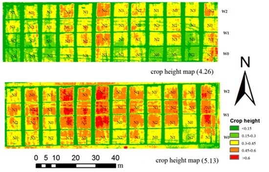
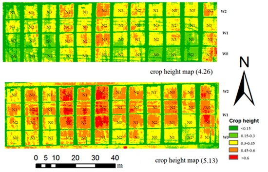
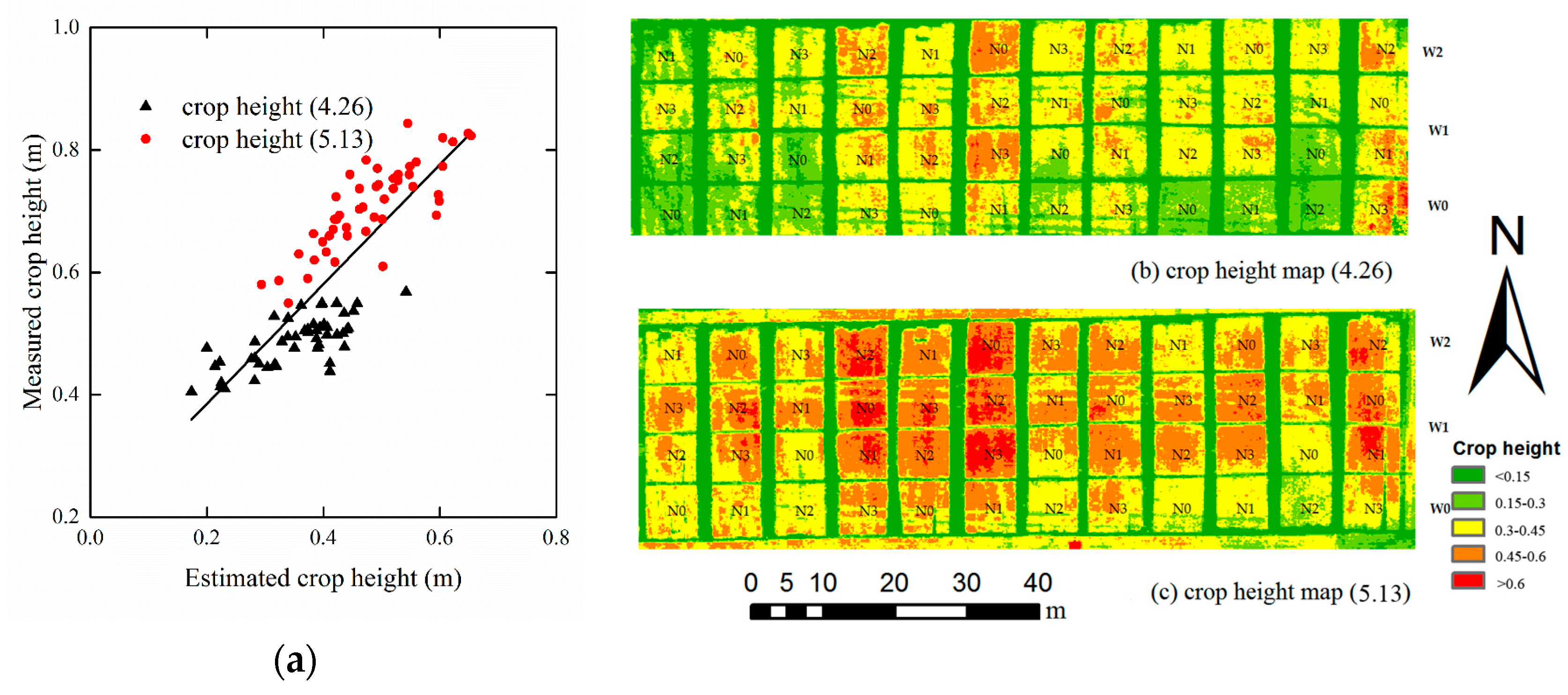
3.1.2. Crop Height Estimation

The height of each plant was extracted using ARCGIS software; estimated and measured crop height is shown in Figure 7a. The linear relationship between estimated and measured crop height was: y = 0.977x + 0.190 (R² = 0.69). Crop height on 26 April and 13 May 2015 is shown in Figure 7b,c. Accuracy verification (Figure 7a) and mapping (Figure 7b,c) demonstrate that the crop height is reliable, although the estimated crop height was smaller than the measured crop height by ~0.19 m; the coefficient of determination for the relationship between the two was high. Figure 7b,c also showed the crop height changing with different growing stage, N and water treatment.

3.2. Biomass Modeling

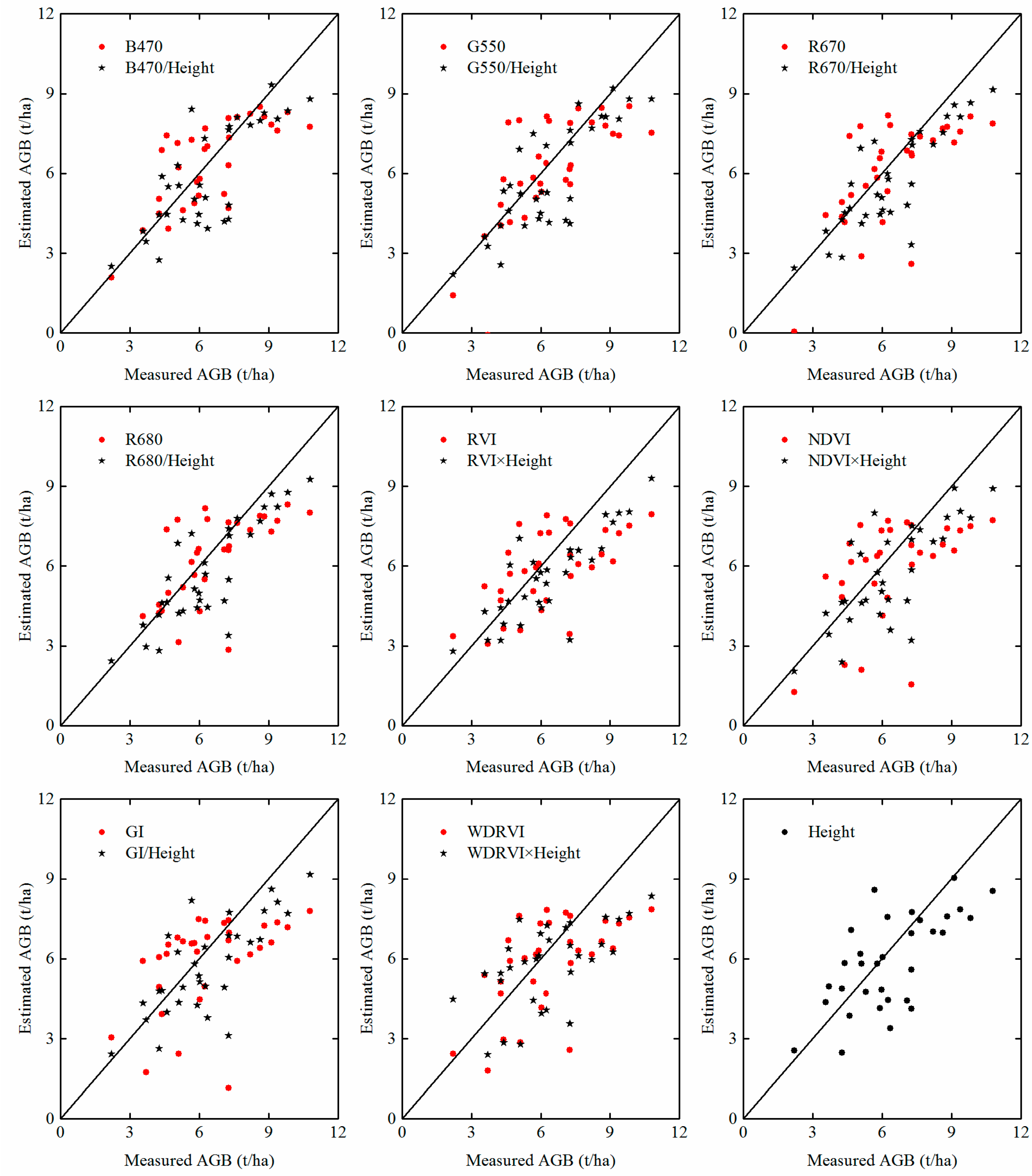
3.2.1. Hyperspectral Model

Winter wheat AGB was significantly correlated with both specific bands and spectral vegetation indices (

Table 2. Correlation coefficients (r) between AGB, specific bands and spectral vegetation indices (n = 96).

Specific Bands and Spectral Vegetation Indices	Correlation Coefficients (r)	Specific Bands and Spectral Vegetation Indices	Correlation Coefficients (r)
B470	−0.74 **	MSAVI	0.21 *
G550	−0.73 **	OSAVI	0.37 **
R670	−0.68 **	WDRVI	0.59 **
R680	−0.69 **	TVI	−0.04 n.s.
Nir800	−0.17 *	DVI1	0.12 n.s.
RVI	0.60 **	DVI2	−0.03 n.s.
NDVI	0.60 **	DVI3	0.12 n.s.
EVI	0.56 **	MTVI1	0.09 n.s.
EVI2	0.19 *	MTVI2	0.27 **
GI	−0.51 **

Note: Probability levels are indicated by n.s., * and ** for ‘not significant’ (up to 0.169), 0.05 (greater than 0.201) and 0.01 (greater than 0.262), respectively. ** r (0.01, 96) = 0.262; * r (0.05, 96) = 0.201.

). Variables in Table 2 with high correlation coefficients (B₄₇₀, G₅₅₀, R₆₇₀, R₆₈₀, RVI, NDVI, GI and WDRVI) were employed to build eight single-parameter AGB estimation models (M1, M2, M3, M4, M5, M6, M7 and M8, respectively) using IBM SPSS19 software (IBM Statistical Product and Service Solutions 19.0, International Business Machines Corporation, New York, NY, USA). The model input parameters, equations and accuracy indices are shown in

Table 3. Details of AGB estimate models.

Models	Details of Models		Modeling Accuracy
	Input Variables	Equation	R2	RMSE (t/ha)	MAE (t/ha)
M1	B470	AGB = −343.928 × B470 + 16.181	0.58	1.48	1.19
M2	G550	AGB = −201.304 × B550 + 15.953	0.56	1.52	1.18
M3	R670	AGB = −212.163 × B670 + 12.687	0.54	1.55	1.23
M4	R680	AGB = −204.084 × B680 + 13.059	0.59	1.47	1.17
M5	RVI	AGB = 0.459 × RVI + 1.467	0.38	1.79	1.53
M6	NDVI	AGB = 25.036 × NDVI − 14.006	0.37	1.81	1.47
M7	GI	AGB = −15.193 × GI + 16.792	0.30	1.91	1.55
M8	WDRVI	AGB = 9.250 × WDRVI + 6.282	0.39	1.79	1.49
M9	Height	AGB = 12.145 × Height + 0.056	0.50	1.62	1.24

Note: Modeling accuracy were calculated using 64 sets of data for AGB models building.

. Crop height also was used to build a single-parameter model (M9), as shown in Table 3.

3.2.2. Crop Height Improved AGB Models

Incorporation of crop height improved the estimation accuracy of AGB models. In this study, specific bands and spectral indices that were positively related to AGB were multiplied by plant height, and those that were negatively related to AGB were divided by crop height to build crop height improved models; as evidenced by the R² (0.58–0.71, 0.54–0.73, 0.56–0.74, 0.59–0.76), RMSE (1.48–1.22 t/ha, 1.52–1.18 t/ha, 1.55–1.16 t/ha, 1.47–1.12 t/ha) and MAE (1.19–0.96 t/ha, 1.18–0.90 t/ha, 1.2–0.85 t/ha, 1.17–0.82 t/ha) values for the HB₄₇₀, HG₅₅₀, HR₆₇₀ and HR₆₈₀ models (

Table 4. Details of the improved AGB model.

Models		Details of Models	Modeling Accuracy
	Description	Equation	R2	RMSE (t/ha)	MAE (t/ha)
HB470	Height/B470	AGB = 0.268 × Height/B470 + 1.163	0.71	1.22	0.96
HG550	Height/G550	AGB = 0.476 × Height/G550 + 0.848	0.73	1.18	0.90
HR670	Height/R670	AGB = 0.246 × Height/R670 + 1.591	0.74	1.16	0.85
HR680	Height/R680	AGB = 0.273 × Height/R680 + 1.567	0.76	1.12	0.82
HRVI	RVI × Height	AGB = 0.723 × RVI × Height + 2.183	0.63	1.39	1.06
HNDVI	NDVI × Height	AGB = 14.300 × NDVI × Height + 0.243	0.58	1.48	1.13
HGI	GI/Height	AGB = 7.072 × GI/Height + 0.821	0.58	1.48	1.16
HWDRVI	WDRVI × Height	AGB = 18.981 × WDRVI × Height + 6.100	0.42	1.75	1.46

Note: Modeling accuracy were calculated using 64 sets of data for AGB models building.

). These models also were validated using field data (Figure 8).

3.2.3. PLSR Methods to Improve the Estimation Accuracy

Incorporation of several spectral indices in Table 3 and Table 4, B₄₇₀, G₅₅₀, R₆₇₀, R₆₈₀, RVI, NDVI, GI, WDRVI, Height, HB₄₇₀, HG₅₅₀, HR₆₇₀, HR₆₈₀, HRVI, HNDVI, HGI and HWDRVI, was combined using the PLSR method (PLSR a in

Table 5. Modeling variables and statistics (R², MAE and RMSE) between the estimated and the measured AGB.

Models	Variables	Modeling			Verification
		R2	RMSE (t/ha)	MAE (t/ha)	R2	RMSE(t/ha)	MAE (t/ha)
PLSR a	HB470, HG550, HR670, HR680, HRVI, HNDVI, HGI and HWDRVI	0.78	1.08	0.83	0.74	1.20	0.96
PLSR b	Height, B470, G550, R670, R680, RVI, NDVI, GI and WDRVI	0.75	1.14	0.87	0.67	1.46	1.14
PLSR c	B470, G550, R670, R680, RVI, NDVI, GI and WDRVI	0.64	0.37	1.09	0.53	1.69	1.20

Note: PLSR a, b and c represent three different combinations for PLSR method. Variables in Table 4 were employed in PLSR a; Variables in Table 3 were employed in PLSR b; Spectral variables in Table 3 were employed in PLSR c respectively.

) to obtain better estimation results. For comparison, the other two groups of variables (PLSR b and PLSR c, list in Table 5) were also employed to calculate AGB using the PLSR method. These PLSR models also were validated using field data. Table 5 shows the modeling precision and verification quality.

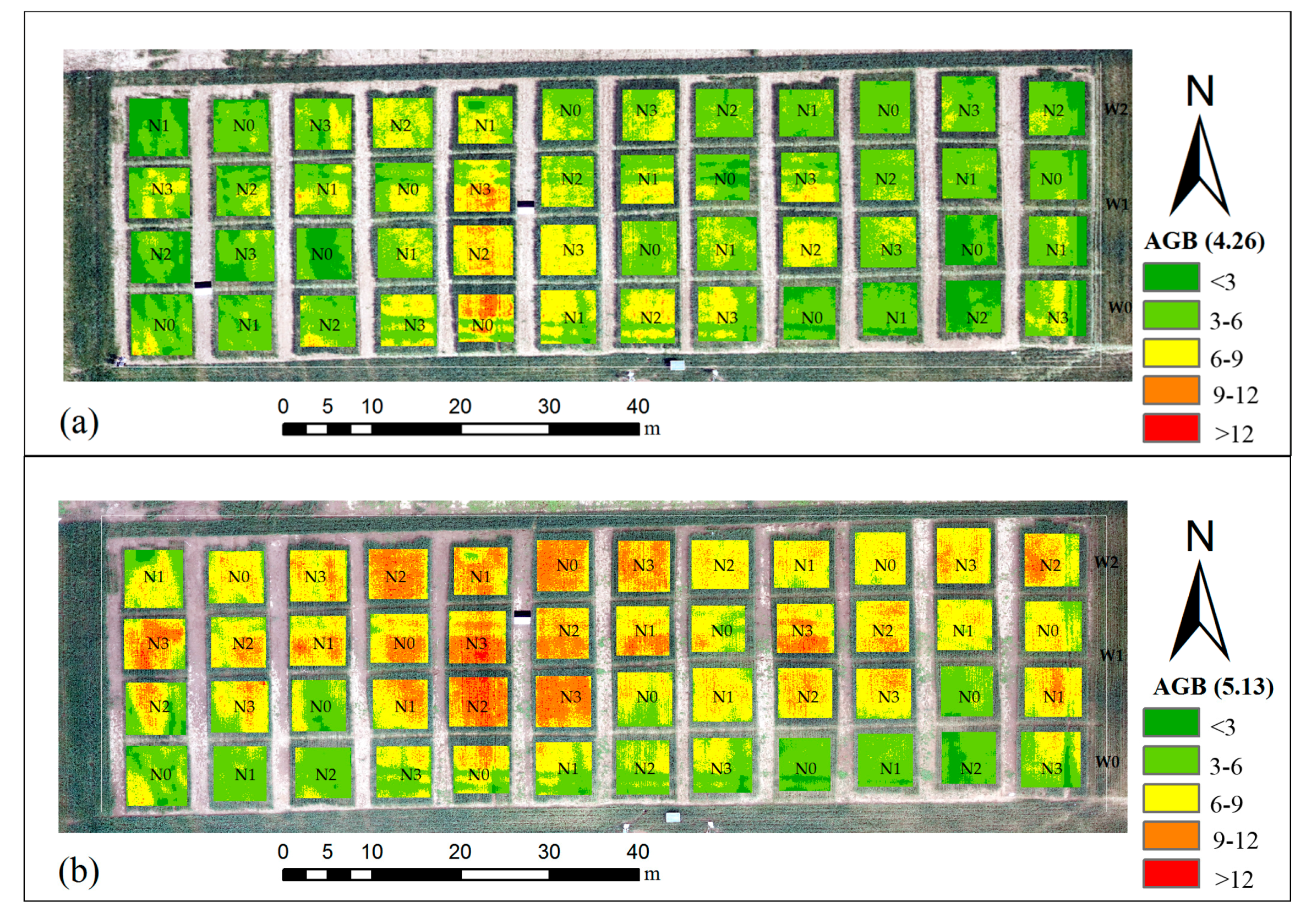
3.2.4. Mapping with Improved Models Based on Crop Height

A map of AGB over the study area was constructed using the HR₆₈₀ model and UHD 185 hyperspectral imagery. An increase in AGB was observed from 26 April–13 May (Figure 9a,b). Furthermore, samples with different levels of irrigation and nitrogen fertilizer were shown to be different in AGB maps; those N0 and W0 plots had lower AGB than N2, N3, W1 and W2. However, there is no strong evidence that the AGB of W2 plots is much higher than W1 plots. The same signs appear on N3 and N2. It is quite clear that excessive fertilize and water alone could not help to increase winter wheat AGB.

4. Discussion

The primary aim of this study was to evaluate the performance of AGB estimation using a snapshot hyperspectral sensor mounted on a UAV platform. Canopy hyperspectral reflectance and crop height were used to construct AGB estimation models.

4.1. Stability and Redundancy of UHD Hyperspectral Data

Aasen et al. [18] showed that the difference between ASD and UHD spectral reflectance is less than 1% in the range of 466–806 nm, but the offset increases rapidly for wavelengths below 466 nm and above 850 nm. We obtained similar hyperspectral data and correlation analysis results of UHD 185, ASD hyperspectral reflectance and AGB (Figure 5 and Figure 6). Both results showed a significant positive approximation between 462 and 800 nm, but a negative approximation between 850 and 882 nm (Figure 5). Correlations between AGB and both ASD and UHD 185 reflectance were high for wavelengths between 462 and 720 nm, but low between 750 and 882 nm (Figure 6). Based on the results, we conclude that the spectrum obtained from the UHD 185 sensor is stable in the visible and near-infrared regions (462–800 nm). These findings about UHD 185 and ASD are consistent with Cui et al. [66] and Gao et al. [65]. The ASD Field Spec 3 spectrometer is designed specifically to have full-range detection capacity (from 350 nm–2500 nm) and provides uniform Vis/NIR/SWIR data collection across the entire solar irradiance spectrum, and its capacity has been publicly recognized. When measuring reflection using the ASD spectrometer, the whiteboard calibration frequency was controllable, but the UHD 185 spectrometer can take this only once before UAV take off. Additionally, the UAV flew fast, leaving the UHD 185 spectrometer an instantaneous time at one location, so it was impossible to obtain enough stable radiation as the ground ASD spectrometer, which also may lead to differences in hyperspectral data.

Redundancy is an important aspect of hyperspectral data that cannot be ignored. The high number of narrow spectral bands results in a high inter-correlation (Figure 10) between them and introduces redundancy into the regression equation [64]. As shown in Figure 10, the band correlation of the two spectrometers is similar. It seems that from the band of 454 nm–882 nm, both ASD and UHD 185 band correlation results can be divided into six groups (a, b, c, d, e, f) by using the correlation value. In previous studies, many methods had been employed for dimensionality reduction, such as principal component analysis, sensitivity analysis and grey relational analysis [25]. In this paper, B470 (blue), G550 (green), R670 (red), R680 (red) and Nir800 (NIR) were selected based on the spectral characteristics of vegetation (Figure 5), sensitivity analysis (Figure 6) and the spectral vegetation indices (Table 1).

4.2. Saturation of Hyperspectral Data and Crop Height Improvement for AGB Estimation

Of the eight single-parameter models we constructed, those based on R₆₇₀ and R₆₈₀ achieved the best accuracy for AGB estimations (Table 3). The estimation accuracy of VI−based models (e.g., RVI, NDVI, GI and WDRVI) was lower than that of models constructed from single specific bands, possibly because the experiments were conducted during the flagging and flowering stages. Sun et al. [67] show that the predictive ability of spectral indices decreased during the middle and late stages of crop growth, while red and near-infrared band-based spectral indices lost sensitivity. During the middle and late stages of crop growth, the wheat reproductive growth was enhanced when the vegetative growth was weakened [68,69], and the winter wheat AGB continued to increase. However, the chlorophyll content of winter wheat leaves was decreased [67], leading to the near-infrared reflectance decreases. In our study, the low correlation results between near-infrared reflectance and biomass correspond with these previous studies. We believe that the reason for the above problem was that the correlation between near-infrared spectral reflectance and crop biomass was decreased for the change of chlorophyll. Therefore, in these wheat growing stages, for biomass estimations based on sole specific bands, spectral indices are infeasible.

AGB estimation models became saturated in the late growth stage of winter wheat using sole spectral information. Many researchers had noticed this problem a long time ago, and they usually switched to using an improved vegetation index [27] or a new type of sensor (such as LiDAR [70] or SAR [71]). Some studies using PLSR can also improve these saturated problems [43], but these models lose physical/biological meaning. Our method is to provide three-dimensional information combining crop height and hyperspectral information to overcome the shortcoming caused by the use of canopy hyperspectral information only. Crop height is an important parameter of winter wheat growth, and many studies have shown that biomass models based on both crop height and spectral indices have high estimation accuracy. Bending et al. [34,35] combined UAV-based spectral vegetation indices (digital camera image data) and crop height (DSM generated by digital camera image) into a biomass estimation model to improve the estimation accuracy of winter wheat AGB. Aasen et al. [18] recently suggested that snapshot hyperspectral sensors are a reliable source for crop height data. Our results support those of these studies and demonstrate that the combing of hyperspectral canopy reflectance and crop height can be used to improve the estimation accuracy of winter wheat AGB. The estimation accuracy of the AGB model based on crop height only (R² = 0.50, RMSE 1.62 t/ha, MAE 1.24 t/ha) was similar to that of models based on single spectral vegetation indices or specific bands. When crop height was combined with spectral vegetation indices or specific bands, the estimation accuracy greatly improved. Models constructed from crop height and HR₆₇₀, HR₆₈₀ or HRVI achieved the best AGB estimation accuracy (

Table 6. Statistics of the coefficient of determination (R²), root mean square error (RMSE) and mean absolute error (MAE) of models in modeling and verification.

Models	R2				RMSE (t/ha)				MAE (t/ha)
	Modeling		Verification		Modeling		Verification		Modeling		Verification
	Before	After	Before	After	Before	After	Before	After	Before	After	Before	After
HB470	0.58	0.71	0.45	0.60	1.48	1.22	1.60	1.41	1.19	0.96	1.33	1.12
HG550	0.56	0.73	0.51	0.66	1.52	1.18	1.50	1.34	1.18	0.90	1.16	1.06
HR670	0.54	0.74	0.51	0.70	1.55	1.16	1.52	1.28	1.23	0.85	1.17	0.99
HR680	0.59	0.76	0.60	0.71	1.47	1.12	1.98	1.27	1.17	0.82	1.41	0.98
HRVI	0.38	0.63	0.46	0.69	1.79	1.39	1.94	1.34	1.53	1.06	1.33	1.10
HNDVI	0.37	0.58	0.36	0.56	1.81	1.48	1.68	1.49	1.47	1.13	1.14	1.17
HGI	0.30	0.58	0.31	0.56	1.91	1.48	2.02	1.48	1.55	1.16	1.68	1.18
HWDRVI	0.39	0.42	0.24	0.35	1.79	1.75	1.94	1.73	1.49	1.46	1.58	1.51

Note: ‘before’ represents only spectral parameters AGB estimation models, and ‘after’ represents crop height improved AGB estimation models.

).

4.3. Two-Band Spectral Vegetation Indices and PLSR Methods

In this paper, by providing three-dimensional information combining crop height and hyperspectral information, the accuracy of spectral vegetation indices (Table 4) has been greatly improved, as well as becoming briefer, simpler and having clearer physical/biological meaning. However, it is also important to recognize that two-band spectral vegetation indices (maybe three-band) make use only of small parts of the information (such NDVI) [72], and the accuracy is lower.

Many previous research works suggested that making full use of hyperspectral information may provide a huge improvement greater than only two-band spectral vegetation indices, such as PLSR [25,43,44,64,72,73], ANN [45,46], SVM [47], RF [48,49], PCR [73] and SMLR [72]. In Table 5 and Table 6, the best two-band spectral vegetation indices (HR680) have been greatly improved with crop height. PLSR still obtained the edge (modeling: R² 0.76−0.78, RMSE 1.12−1.02, MAE 0.82−0.83; verification: R² 0.71−0.74, RMSE 1.27−1.20, MAE 0.98−0.96). These studies about hyperspectral and PLSR are consistent with Atzberger et al. [72], Mirzaie et al. [73] and Fu et al. [43].

However, using these powerful techniques/methods was limited by the complex models, for example being difficult to express in the form of a simple formula. More importantly, the models lose the crucial physical/biological meaning. Additionally, airborne hyperspectral sensors are more expensive than narrow band multispectral sensors, and two-band spectral vegetation indices may have advantages in these applications.

4.4. Crop Height and Ground Elevation Control Points

DSM, DEM and crop height values were extracted without using ground elevation control points; therefore, crop height results may still be impacted without the ground elevation control point. Elevation in DEM was measured based on multiple bare soil points from the DSM, and an interpolation method (kriging) was used to obtain the DEM. Without the help of ground elevation control points [74], these crop height values cannot be highly accurate, and thus, our study could be improved by using stable ground elevation control points.

5. Conclusions

Images from the UHD 185 hyperspectral sensor combined imagery and hyperspectral information. We constructed AGB estimation models based on crop height, specific bands and spectral vegetation indices, which are extremely sensitive to winter wheat growth. Eight models based on specific bands and vegetation indices were established (Table 3), as well as eight models based on crop height combined with specific bands and vegetation indices (Table 4). The results show that the combination of hyperspectral canopy reflectance data and crop height can be used to improve the estimation accuracy of winter wheat AGB (Table 6, Figure 8).

To make full use of hyperspectral data, suitable methods have to be used. In this study, concerning the two-band spectral vegetation indices (maybe three-band) making use only of small parts of the hyperspectral information, the existence of PLSR is particularly necessary to achieve higher accuracy.

The UHD 185 sensor can improve AGB monitoring performance by providing hyperspectral and stereo imagery. Crop height obtained from this new spectrometer can greatly improve biomass estimation accuracy and mapping applications (Figure 9), which are critical for guiding agricultural management.

References

1. Wang, L.; Zhou, X.; Zhu, X.; Dong, Z.; Guo, W. Estimation of biomass in wheat using random forest regression algorithm and remote sensing data. Crop J. 2016, 4, 212–219. [Google Scholar] [CrossRef]
2. Hensgen, F.; Bühle, L.; Wachendorf, M. The effect of harvest, mulching and low-dose fertilization of liquid digestate on above ground biomass yield and diversity of lower mountain semi-natural grasslands. Agric. Ecosyst. Environ. 2016, 216, 283–292. [Google Scholar] [CrossRef]
3. Huang, J.; Sedano, F.; Huang, Y.; Ma, H.; Li, X.; Liang, S.; Tian, L.; Zhang, X.; Fan, J.; Wu, W. Assimilating a synthetic Kalman filter leaf area index series into the WOFOST model to improve regional winter wheat yield estimation. Agric. For. Meteorol. 2016, 216, 188–202. [Google Scholar] [CrossRef]
4. He, L.; Chen, Z.; Jiang, Z.; Wen, B.; Wu, W.B.; Ren, J.; Liu, B.; Tuya, H. Comparative analysis of GF-1, HJ-1, and Landsat-8 data for estimating the leaf area index of winter wheat. J. Integr. Agric. 2016, 16, 266–285. [Google Scholar] [CrossRef]
5. Soudani, K.; François, C.; Maire, G.L.; Dantec, V.; Dufrêne, E. Comparative analysis of IKONOS, SPOT, and ETM+ data for leaf area index estimation in temperate coniferous and deciduous forest stands. Remote Sens. Environ. 2006, 102, 161–175. [Google Scholar] [CrossRef]
6. Jibo, Y.; Guijun, Y.; Haikuan, F. Comparative of remote sensing estimation models of winter wheat biomass based on random forest algorithm. Trans. Chin. Soc. Agric. Eng. 2016, 32, 175–182. [Google Scholar] [CrossRef]
7. Campos, M.; García, F.J.; Camps, G.; Grau, G.; Nutini, F.; Crema, A.; Boschetti, M. Multitemporal and multiresolution leaf area index retrieval for operational local rice crop monitoring. Remote Sens. Environ. 2016, 187, 102–118. [Google Scholar] [CrossRef]
8. Dong, Y.; Wang, J.; Li, C.; Yang, G. Comparison and Analysis of Data Assimilation Algorithms for Predicting the Leaf Area Index of Crop Canopies. IEEE J. Sel. Top. Appl. Earth Obs. Remote Sens. 2013, 6, 188–201. [Google Scholar] [CrossRef]
9. Houghton, A.; Hall, F.; Goetz, J. Importance of biomass in the global carbon cycle. J. Geophys. Res. Biogeosci. 2009, 114, 1–13. [Google Scholar] [CrossRef]
10. Badhwar, D.; Macdonald, B. Satellite-derived leaf-area-index and vegetation maps as input to global carbon cycle models-a hierarchical approach. Int. J. Remote Sens. 1986, 7, 265–281. [Google Scholar] [CrossRef]
11. Liu, R.; Chen, M.; Liu, J.; Deng, F.; Sun, R. Application of a new leaf area index algorithm to China’s landmass using MODIS data for carbon cycle research. J. Environ. Manag. 2007, 85, 649–658. [Google Scholar] [CrossRef] [PubMed]
12. Chen, Y.; Luo, Y.; Reich, B.; Searle, B.; Biswas, R. Climate change−associated trends in net biomass change are age dependent in western boreal forests of canada. Ecol. Lett. 2016, 19, 1150–1158. [Google Scholar] [CrossRef] [PubMed]
13. Chen, Y.; Luo, Y. Net aboveground biomass declines of four major forest types with forest ageing and climate change in western canada’s boreal forests. Glob. Chang. Biol. 2015, 21, 3675–3684. [Google Scholar] [CrossRef] [PubMed]
14. Adler, O.; Rosenberger, A.; Malberger, E.; Koenig, B.; Peleg, H. Relative contributions of climate change, stomatal closure, and leaf area index changes to 20th and 21st century runoff change: A modelling approach using the Organizing Carbon and Hydrology in Dynamic Ecosystems (ORCHIDEE) land surface model. J. Geophys. Res. Atmos. 2010, 115, 1383–1392. [Google Scholar] [CrossRef]
15. Sankaran, S.; Khot, R.; Espinoza, Z.; Jarolmasjed, S.; Sathuvalli, R.; Vandemark, J.; Miklas, N.; Carter, H.; Pumphrey, O.; Knowles, R. Low-altitude, high-resolution aerial imaging systems for row and field crop phenotyping: A review. Eur. J. Agron. 2015, 70, 112–123. [Google Scholar] [CrossRef]
16. Zarcotejada, J.; Guilléncliment, L.; Hernándezclemente, R.; Catalina, A.; González, R.; Martín, P. Estimating leaf carotenoid content in vineyards using high resolution hyperspectral imagery acquired from an unmanned aerial vehicle (UAV). Agric. For. Meteorol. 2013, 171–172, 281–294. [Google Scholar] [CrossRef]
17. Bareth, G.; Aasen, H.; Bendig, J.; Gnyp, L.; Bolten, A.; Jung, A.; Michels, R.; Soukkamäki, J. Low-weight and UAV-based Hyperspectral Full-frame Cameras for Monitoring Crops: Spectral Comparison with Portable Spectroradiometer Measurements. Photogramm. Fernerkund. Geoinf. 2015, 69–79. [Google Scholar] [CrossRef]
18. Aasen, H.; Burkart, A.; Bolten, A.; Bareth, G. Generating 3D hyperspectral information with lightweight UAV snapshot cameras for vegetation monitoring: From camera calibration to quality assurance. Isprs J. Photogramm. Remote Sens. 2015, 108, 245–259. [Google Scholar] [CrossRef]
19. Uhd-185-Firefly. Available online: http://cubert-gmbh.com/uhd-185-firefly/ (accessed on 15 May 2017).
20. Rouse, J.; Haas, H.; Schell, A.; Deering, W.; Harlan, C. Monitoring the Vernal Advancement of Retrogradation (Green Wave Effect) of Natural Vegetation; Type III, Final Report; NASA: Washington, DC, USA, 1974; pp. 1–371. Available online: https://ntrs.nasa.gov/archive/nasa/casi.ntrs.nasa.gov/19730009608.pdf (accessed on 15 May 2017).
21. Huete, A. A soil-adjusted vegetation index (SAVI). Remote Sens. Environ. 1988, 25, 295–309. [Google Scholar] [CrossRef]
22. Jordan, F. Derivation of Leaf−Area Index from Quality of Light on the Forest Floor. Ecology 1969, 50, 663–666. [Google Scholar] [CrossRef]
23. Elmore, J.; Mustard, F.; Manning, J. Quantifying vegetation change in semiarid environments: Precision and accuracy of spectral mixture analysis and the normalized difference vegetation index. Remote Sens. Environ. 2000, 73, 87–102. [Google Scholar] [CrossRef]
24. Jin, L.; Diao, Y.; Xiao, H.; Wang, Y.; Chen, B.; Wang, R. Estimation of wheat agronomic parameters using new spectral indices. PLoS ONE 2013, 8, e72736. [Google Scholar] [CrossRef] [PubMed]
25. Jin, X.; Xu, X.; Song, X.; Li, Z.; Wang, J.; Guo, W. Estimation of leaf water content in winter wheat using grey relational analysis-partial least squares modeling with hyperspectral data. Agron. J. 2013, 105, 1385–1392. [Google Scholar] [CrossRef]
26. Gitelson, A. Wide dynamic range vegetation index for remote quantification of biophysical characteristics of vegetation. J. Plant Physiol. 2004, 161, 165–173. [Google Scholar] [CrossRef] [PubMed]
27. Pu, R.; Gong, P. Wavelet transform applied to eo-1 hyperspectral data for forest lai and crown closure mapping. Remote Sens. Environ. 2004, 91, 212–224. [Google Scholar] [CrossRef]
28. Delegido, J.; Fernandez, G.; Gandia, S.; Moreno, J. Retrieval of chlorophyll content and lai of crops using hyperspectral techniques: Application to proba/chris data. Int. J. Remote Sens. 2008, 29, 7107–7127. [Google Scholar] [CrossRef]
29. Meroni, M.; Colombo, R.; Panigada, C. Inversion of a radiative transfer model with hyperspectral observations for lai mapping in poplar plantations. Remote Sens. Environ. 2004, 92, 195–206. [Google Scholar] [CrossRef]
30. Calderón, R.; Navas, J.A.; Lucena, C.; Zarco, P. High-resolution airborne hyperspectral and thermal imagery for early detection of Verticillium wilt of olive using fluorescence, temperature and narrow-band spectral indices. Remote Sens. Environ. 2013, 139, 231–245. [Google Scholar] [CrossRef]
31. Li, W.; Niu, Z.; Chen, H.; Li, D.; Wu, M.; Zhao, W. Remote estimation of canopy height and aboveground biomass of maize using high-resolution stereo images from a low-cost unmanned aerial vehicle system. Ecol. Indic. 2016, 67, 637–648. [Google Scholar] [CrossRef]
32. Gago, J.; Douthe, C.; Coopman, E.; Gallego, P.; Ribas, M.; Flexas, J.; Escalona, J.; Medrano, H. UAVs challenge to assess water stress for sustainable agriculture. Agric. Water Manag. 2015, 153, 9–19. [Google Scholar] [CrossRef]
33. Ribeiro, K.; Hernandez, D.; Ballesteros, R.; Moreno, M. Approximate georeferencing and automatic blurred image detection to reduce the costs of UAV use in environmental and agricultural applications. Biosyst. Eng. 2016, 151, 308–327. [Google Scholar] [CrossRef]
34. Bendig, J.; Bolten, A.; Bennertz, S.; Broscheit, J.; Eichfuss, S.; Bareth, G. Estimating biomass of barley using crop surface models (csms) derived from uav-based rgb imaging. Remote Sens. 2014, 11, 10395–10412. [Google Scholar] [CrossRef]
35. Bendig, J.; Yu, K.; Aasen, H.; Bolten, A.; Bennertz, S.; Broscheit, J.; Gnyp, M.; Bareth, G. Combining UAV-based plant height from crop surface models, visible, and near infrared vegetation indices for biomass monitoring in barley. Int. J. Appl. Earth Obs. Geoinf. 2015, 39, 79–87. [Google Scholar] [CrossRef]
36. Jannoura, R.; Brinkmann, K.; Uteau, D.; Bruns, C.; Joergensen, R. Monitoring of crop biomass using true colour aerial photographs taken from a remote controlled hexacopter. Biosyst. Eng. 2014, 129, 341–351. [Google Scholar] [CrossRef]
37. Berni, J.; Zarcotejada, P.; Sepulcrecantó, G.; Fereres, E.; Villalobos, F. Mapping canopy conductance and CWSI in olive orchards using high resolution thermal remote sensing imagery. Remote Sens. Environ. 2009, 113, 2380–2388. [Google Scholar] [CrossRef]
38. Vonbueren, S.; Burkart, A.; Hueni, A.; Rascher, U.; Tuohy, M.; Yule, I. Deploying four optical UAV-based sensors over grassland: Challenges and limitations. Biogeosciences 2015, 12, 163–175. [Google Scholar] [CrossRef]
39. Vega, F.; Ramírez, F.; Saiz, M.; Rosúa, F. Multi-temporal imaging using an unmanned aerial vehicle for monitoring a sunflower crop. Biosyst. Eng. 2015, 132, 19–27. [Google Scholar] [CrossRef]
40. Honkavaara, E.; Saari, H.; Kaivosoja, J.; Nen, L.; Hakala, T.; Litkey, P.; Kynen, J.; Pesonen, L. Processing and Assessment of Spectrometric, Stereoscopic Imagery Collected Using a Lightweight UAV Spectral Camera for Precision Agriculture. Remote Sens. 2013, 5, 5006–5039. [Google Scholar] [CrossRef]
41. Moshou, D.; Bravo, C.; Oberti, R.; West, J.; Bodria, L.; McCartney, A.; Ramon, H. Plant disease detection based on data fusion of hyper-spectral and multi-spectral fluorescence imaging using Kohonen maps. Real-Time Imaging 2005, 11, 75–83. [Google Scholar] [CrossRef]
42. Liu, J.; Zhao, C.; Yang, G.; Yu, H.; Zhao, X.; Xu, B.; Niu, Q. Review of field-based phenotyping by unmanned aerial vehicle remote sensing platform. Trans. Chin. Soc. Agric. Eng. 2016, 32, 98–106. [Google Scholar] [CrossRef]
43. Fu, Y.Y.; Yang, G.J.; Wang, J.H.; Song, X.Y.; Feng, H.K. Winter wheat biomass estimation based on spectral indices, band depth analysis and partial least squares regression using hyperspectral measurements. Comput. Electr. Agric. 2014, 100, 51–59. [Google Scholar] [CrossRef]
44. Nguyen, H.T.; Lee, B.W. Assessment of rice leaf growth and nitrogen status by hyperspectral canopy reflectance and partial least square regression. Eur. J. Agron. 2006, 24, 349–356. [Google Scholar] [CrossRef]
45. Yang, G.J.; Zhao, C.J.; Xing, Z.R. LAI inversion of spring wheat based on PROBA/CHRIS hyperspectral multi-angular data and PROSAIL model. Trans. CSAE 2011, 27, 88–94. [Google Scholar] [CrossRef]
46. Atzberger, C. Object-based retrieval of biophysical canopy variables using artificial neural nets and radiative transfer models. Remote Sens. Environ. 2004, 93, 53–67. [Google Scholar] [CrossRef]
47. Yang, X.H.; Huang, J.F.; Wang, X.Z.; Wang, F.M. The estimation model of rice leaf area index using hyperspectral data based on support vector machine. Spectrosc. Spectr. Anal. 2008, 28, 1837. [Google Scholar] [CrossRef]
48. Han, Z.Y.; Zhu, X.C.; Fang, X.Y.; Wang, Z.Y.; Wang, L.; Zhao, G.X. Hyperspectral estimation of apple tree canopy lai based on svm and rf regression. Spectrosc. Spectr. Anal. 2016, 36, 800–805. [Google Scholar] [CrossRef]
49. Yuan, H.H.; Yang, G.J.; Li, C.C.; Wang, Y.J.; Liu, J.G.; Yu, H.Y.; Feng, H.K.; Xu, B.; Zhao, X.Q.; Yang, X.D. Retrieving Soybean Leaf Area Index from Unmanned Aerial Vehicle Hyperspectral Remote Sensing: Analysis of RF, ANN, and SVM Regression Models. Remote Sens. 2017, 9, 309. [Google Scholar] [CrossRef]
50. China Meteorological Data. Available online: http://data.cma.cn/ (accessed on 15 May 2017).
51. National Engineering Research Center for Information Technology in Agriculture. Available online: http://www.nercita.org.cn/English/e_index.asp (accessed on 15 May 2017).
52. DJI. Available online: https://www.dji.com/ (accessed on 15 May 2017).
53. Agisoft. Available online: http://www.agisoft.com/ (accessed on 15 May 2017).
54. ENVI. Available online: http://www.harrisgeospatial.com/ProductsandSolutions/GeospatialProducts/ENVI.aspx (accessed on 15 May 2017).
55. Pu, R.; Gong, P. Hyperspectral Remote Sensing of Vegetation Bioparameters. In Advances in Environmental Remote Sensing: Sensors, Algorithm, and Application; Weng, Q., Ed.; CRC Press: Boca Raton, FL, USA, 2011; pp. 101–142. [Google Scholar]
56. Huete, A.; Didan, K.; Miura, T.; Rodriguez, E.; Gao, X.; Ferreira, L. Overview of the radiometric and biophysical performance of the MODIS vegetation indices. Remote Sens. Environ. 2002, 83, 195–213. [Google Scholar] [CrossRef]
57. Jiang, Z.; Huete, A.; Didan, K.; Miura, T. Development of a two-band enhanced vegetation index without a blue band. Remote Sens. Environ. 2008, 112, 3833–3845. [Google Scholar] [CrossRef]
58. Zarco, P.; Rueda, C.; Ustin, L. Water content estimation in vegetation with MODIS reflectance data and model inversion methods. Remote Sens. Environ. 2003, 85, 109–124. [Google Scholar] [CrossRef]
59. Qi, J.; Chehbouni, A.; Huete, A.; Kerr, H.; Sorooshian, S. A modified soil adjusted vegetation index. Remote Sens. Environ. 1994, 48, 119–126. [Google Scholar] [CrossRef]
60. Rondeaux, G.; Steven, M.; Baret, F. Optimization of soil−adjusted vegetation indices. Remote Sens. Environ. 1996, 55, 95–107. [Google Scholar] [CrossRef]
61. Haboudane, D.; Miller, J.; Pattery, E.; Zarco, P.; Strachan, B. Hyperspectral vegetation indices and novel algorithms for predicting green LAI of crop canopies: Modeling and validation in the context of precision agriculture. Remote Sens. Environ. 2004, 90, 337–352. [Google Scholar] [CrossRef]
62. Broge, H.; Leblanc, E. Comparing prediction power and stability of broadband and hyperspectral vegetation indices for estimation of green leaf area index and canopy chlorophyll density. Remote Sens. Environ. 2000, 76, 156–172. [Google Scholar] [CrossRef]
63. Wold, H. Estimation of Principal Components and Related Models by Iterative Least Squares. J. Multivar. Anal. 1966, 1, 391–420. [Google Scholar]
64. Darvishzadeh, R.; Skidmore, A.; Schlerf, M.; Atzberger, C.; Corsi, F.; Cho, M. Lai and chlorophyll estimation for a heterogeneous grassland using hyperspectral measurements. Isprs J. Photogramm. Remote Sens. 2008, 63, 409–426. [Google Scholar] [CrossRef]
65. Gao, L.; Yang, G.; Yu, H.; Xu, B.; Zhao, X.; Dong, J.; Ma, Y. Retrieving winter wheat leaf area index based on unmanned aerial vehicle hyperspectral remoter sensing. Trans. Chin. Soc. Agric. Eng. 2016, 32, 113–120. [Google Scholar] [CrossRef]
66. Cui, J.; Zhang, S.; Zhang, J. Determining surface magnetic susceptibility of loess-paleosol sections based on spectral features: Application to a UHD 185 hyperspectral image. Int. J. Appl. Earth Obs. Geoinf. 2016, 50, 159–169. [Google Scholar] [CrossRef]
67. Sun, H.; Li, M.; Zhao, Y.; Zhang, Y.; Wang, X.; Li, X. The spectral characteristics and chlorophyll content at winter wheat growth stages. Spectrosc. Spectr. Anal. 2010, 30, 192–196. [Google Scholar] [CrossRef]
68. Wang, J.; Zhao, C.; Huang, W. Fundamental and Application of Quantitative Remote Sensing in Agric, 1st ed.; Science China Press: Beijing, China, 2008; pp. 4–5. [Google Scholar]
69. Yang, G. Cropland Radiative Transfer Model and Remote Sensing Imaging Simulation, 1st ed.; China Meteorological Press: Beijing, China, 2012; pp. 109–110. [Google Scholar]
70. Wallace, L.; Musk, R.; Lucieer, A. An Assessment of the Repeatability of Automatic Forest Inventory Metrics Derived From UAV-Borne Laser Scanning Data. IEEE Trans. Geosci. Remote Sens. 2014, 52, 60–71. [Google Scholar] [CrossRef]
71. Iiames, J.; Marks, W.; Lunetta, R.; Khorram, S.; Mace, T. Basal Area and Biomass Estimates of Loblolly Pine Stands using L-Band UAVSAR. Photogramm. Eng. Remote Sens. 2014, 80, 33–42. [Google Scholar] [CrossRef]
72. Atzberger, C.; Guérif, M.; Baret, F.; Werner, W. Comparative analysis of three chemometric techniques for the spectroradiometric assessment of canopy chlorophyll content in winter wheat. Comput. Electr. Agric. 2010, 73, 165–173. [Google Scholar] [CrossRef]
73. Mirzaie, M.; Darvishzadeh, R.; Shakiba, A.; Matkan, A.A.; Atzberger, C.; Skidmore, A. Comparative analysis of different uni-and multi-variate methods for estimation of vegetation water content using hyper-spectral measurements. Int. J. Appl. Earth Obs. Geoinf. 2014, 26, 1–11. [Google Scholar] [CrossRef]
74. Jianqing, Z.; Li, P.; Shugen, W. Photogrammetry, 3rd ed.; Wuhan University Press: Wuhan, China, 2009; pp. 74–96. [Google Scholar]
Figure 1. Location of the study area.
Remotesensing 09 00708 g001
Figure 2. Experimental details. Plants were divided into three groups, with a total of 16 winter wheat plants per group. Planting area was 6 × 8 m, and each group received different fertilization and irrigation treatments.
Remotesensing 09 00708 g002
Figure 3. Components of the UHD 185 hyperspectral system: (a) reinforcement notebook computer and ground control station; (b) remote controller; (c) UHD 185 Firefly spectrometer.
Remotesensing 09 00708 g003
Figure 4. 3D surface view of the crop height map.
Remotesensing 09 00708 g004
Figure 5. Canopy reflectance measured by the UHD 185 and ASD from 462–882 nm during the flagging stage. Grey solid and dashed lines represent the reflectance of Plot 4-1 measured by the ASD and UHD 185, respectively; black solid and dashed lines represent the reflectance of Plot 9-1 measured by the ASD and UHD 185, respectively; red solid and dashed lines represent the reflectance of Plot 2-2 measured by the ASD and UHD 185, respectively.
Remotesensing 09 00708 g005
Figure 6. Correlation analysis between ASD spectral reflectance with AGB, UHD 185 spectral reflectance with AGB.
Remotesensing 09 00708 g006
Figure 7. Crop height: (a) estimated and measured crop height; (b) crop height on 26 April 2015; (c) crop height on 13 May 2015.
Remotesensing 09 00708 g007
Figure 8. Comparison of measured and improved model estimated AGB.
Remotesensing 09 00708 g008
Figure 9. AGB Map: (a) AGB during the flagging stage (26 April 2015); (b) AGB during the flowering stage (13 May 2015); Dark and light green regions of the image (Figure 9a,b, AGB < 6) correspond to low crop growth, yellow regions (Figure 9a,b, 6 < AGB < 9) correspond to normal crop growth, and orange and red regions (Figure 9a,b, AGB > 9) correspond high crop growth.
Remotesensing 09 00708 g009
Figure 10. The correlation coefficients among different bands of the UHD 185 and ASD spectrometer. Mostly, Groups a, b and c represent band correlation values greater than 0.9; Group d represents correlation values at 0.7−0.9; the correlation values of Groups e and f are less than 0.4.
Remotesensing 09 00708 g010