Assessing the Value of UAV Photogrammetry for Characterizing Terrain in Complex Peatlands


Department of Geography, University of Calgary, Calgary, AB T2N 1N4, Canada
*
Author to whom correspondence should be addressed.
Remote Sens. 2017, 9(7), 715; https://doi.org/10.3390/rs9070715
Submission received: 26 April 2017
/
Revised: 13 June 2017
/
Accepted: 6 July 2017
/
Published: 12 July 2017
(This article belongs to the Section Forest Remote Sensing)
Abstract
:Microtopographic variability in peatlands has a strong influence on greenhouse gas fluxes, but we lack the ability to characterize terrain in these environments efficiently over large areas. To address this, we assessed the capacity of photogrammetric data acquired from an unmanned aerial vehicle (UAV or drone) to reproduce ground elevations measured in the field. In particular, we set out to evaluate the role of (i) vegetation/surface complexity and (ii) supplementary LiDAR data on results. We compared remote-sensing observations to reference measurements acquired with survey grade GPS equipment at 678 sample points, distributed across a 61-hectare treed bog in northwestern Alberta, Canada. UAV photogrammetric data were found to capture elevation with accuracies, by root mean squares error, ranging from 14–42 cm, depending on the state of vegetation/surface complexity. We judge the technology to perform well under all but the most-complex conditions, where ground visibility is hindered by thick vegetation. Supplementary LiDAR data did not improve results significantly, nor did it perform well as a stand-alone technology at the low densities typically available to researchers.
1. Introduction
Fine-scale variability in elevation, commonly referred to as microtopography, is an important factor in the distribution of greenhouse gas (GHG) flux across peatland ecosystems [1,2,3,4,5,6,7]. Consequently, including microtopographic information in carbon-balance models is often recommended as a means of improving model accuracies [6,8,9,10,11]. Most commonly, microtopographic data are acquired via terrestrial surveys using real-time kinematic global navigation satellite system (RTK GNSS) equipment, which are capable of centimeter accuracies [12,13]. However, terrestrial surveys are limited by high costs and personnel requirements, and do not scale well over large areas [13].
Recently, researchers have used photogrammetric data from unmanned aerial vehicles (UAVs) to acquire detailed microtopographic data in a variety of terrestrial settings, suggesting that the technology might provide an attractive alternative to traditional ground surveys in peatlands. Using standard consumer-grade cameras, UAVs can produce high-density point clouds (100 s of points per m2) and ultra-high resolution orthomosaics with modern photogrammetry principles and structure from motion (SfM) computer-vision software [14]. Roosevelt et al. [13] found UAV photogrammetry to be one order of magnitude more labor-efficient and at least two orders of magnitude more detailed (in terms of data density) than RTK GNSS surveys for microtopographic archaeology surveys in western Turkey. Working in gently sloping, sparsely vegetated hills interspersed with olive orchards, the authors reported vertical root mean squares error (RMSE) values of 21 cm compared to ground control points (GCPs). Lucieer et al. [15] reported even better RMSE accuracies of 4 cm in microtopographic surveys of East Antarctic moss beds with UAV photogrammetry. Using an alternative multispectral approach, Lehmann et al. [11] classified vegetation species and microforms with high accuracy (>80%) using UAV-derived color infrared (CIR) imagery of a South Patagonian peatland. While this research did not make use of photogrammetric elevation data, the authors suggested that doing so would have increased classification accuracies even further [11].
Building on these promising early studies, there is a need to evaluate the performance of UAV photogrammetry in other, more complex environments. The peatlands of the boreal zone contain globally significant carbon stocks, and are an essential target for climate-change studies [16,17]. However, terrain modeling in these environments is expected to be more challenging for UAV photogrammetry, given the complexity of the surfaces and the presence of vascular vegetation, both of which can negatively affect the performance of SfM workflows. For example, Javernick et al. [18] assessed photogrammetric point clouds from UAVs for modelling the topography of a shallow braided river in New Zealand, and found vegetation cover to negatively affect results. Vertical accuracies fell from 17 cm (RMSE) in bare areas to 78 cm in areas of vegetation, due to the inconsistent ability of passive photography to penetrate the vegetation canopy [18]. Similarly, elevated wind speeds have been shown to decrease UAV data quality in vegetated areas due to movement of the canopy surface (increased photo blurriness), and interference with UAV positioning and orientation during image capture [19,20]. In some cases, this effect can be severe. For example, Zainuddin et al. [20] found excessive tree leaf movement due to strong winds during UAV data acquisition caused ten trees to be completely missed in the produced point cloud, and increased uncertainty in ground surface elevations around modeled trees. This ultimately resulted in a poor quality, and non-useful 3D model for estimating canopy heights (69.6 cm RMSE; [20]).
Additional challenges associated with elevation changes, presence of standing water and image-texture homogeneity have also been noted in the literature. For example, Mancini et al. [21] compared UAV point clouds from passive photogrammetry to those derived from a terrestrial light detection and ranging (LiDAR) scanning system, an active (laser) technology, over sand dunes in Italy. The authors found photogrammetric point density to decrease in flat bare areas, due to the inability of the SfM feature-matching algorithm to reliably identify tie points. Areas of dense vegetation were excluded from this assessment, though sparse vegetation (15- to 20-cm patches) were included in the linearly interpolated DSM surfaces and reportedly influenced overall accuracy (11 cm RMSE; [21]). Similar results have been reported in areas of standing water, where the surface is too homogenous to accurately locate tie points, or where variations in reflectance across the water surface cause SfM algorithms to incorrectly estimate point locations [22,23,24].
One potentially promising strategy involves combining passive photogrammetric data (high point density, but limited canopy penetrating abilities) with airborne LiDAR, which typically has lower densities but an enhanced capacity to penetrate vegetation. LiDAR has proven to be highly accurate in estimating ground surface elevations within bare, flat areas [25,26], though canopy interference and low point densities are likely to decrease estimated surface accuracies in more complex environments. However, these data have yet to be widely assessed in a peatlands context.
The goal of this research is to assess the value of UAV photogrammetry for characterizing terrain in vegetated peatlands in the Canadian boreal forest. In this study, we worked in a treed-bog ecosystem in North-West Alberta, Canada that displayed a wide range of complexity, from relatively flat, open areas to a mixture of highly undulating and treed zones. Our objective was to assess the accuracy of photogrammetric point clouds for capturing terrain elevation under a variety of vegetation/surface-complexity conditions, paving the way for future work aimed at classifying peatland microtopographic landforms (hummocks and hollows). In addition, we also assessed the value of supplementary LiDAR data over the same gradient of complexity. To achieve these objectives, we created three-dimensional point clouds from three different remote sensing data sets: (i) UAV photogrammetry; (ii) LiDAR; and (iii) merged UAV photogrammetry + LiDAR. The accuracy of these data sets was assessed using terrestrial surveys conducted in the field.
2. Materials and Methods
2.1. Study Area
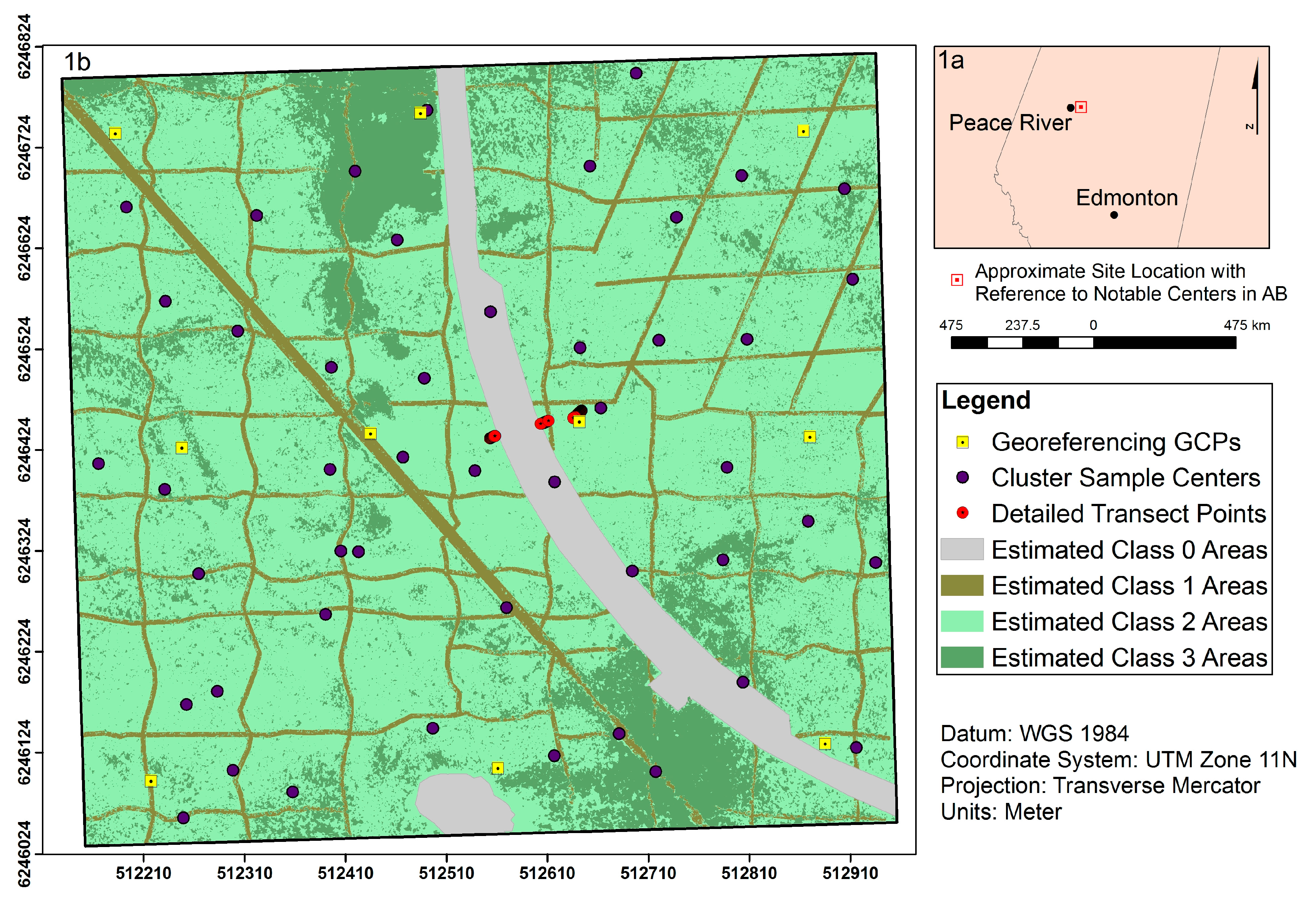
The study site is a 61-hectare section of treed bog located approximately 35 km northeast of Peace River, Alberta, Canada (Figure 1). The site is a mixture of open bog, mostly covered by mosses and lichens (e.g., Sphagnum mosses, big red stem moss (Pleurozium schreberi), stair step moss (Hylocomium splendens), fairy’s puke (lcmadophila ericetorum), and reindeer lichens (Cladina stellaris, C. rangiferina, C. mitis)), shrubby bog with dispersed to moderately dense shrubs (e.g., Labrador tea (Rhododendron groenlandicum) and Lignonberry (Vaccinium vitis-idaea)), and moderately dense treed bog dominated by black spruce (Picea mariana). In the few marginal fen-like areas, tamarack (Larix laricina) and willow (Salix spp.) are present. Upland areas are dominated by mixed forest including balsam poplar (Populus balsamifera), trembling aspen (Populus tremuloides) and white spruce (Picea glauca). Black spruce, the dominant tree species in boreal bog ecosystems, do generally not produce large-diameter canopies. However, these trees are dense enough in some portions of our study site to obscure the ground surface from passive sensors, as are shrubby vegetation cover types such as Labrador tea.
Microforms (hummocks and hollows) are well established in undisturbed bog portions of the study area, and generally occur at scales between 30 and 100 cm. However, a network of linear disturbances, including seismic lines, a pipeline right-of-way (ROW), and a roadway, also transect the site.
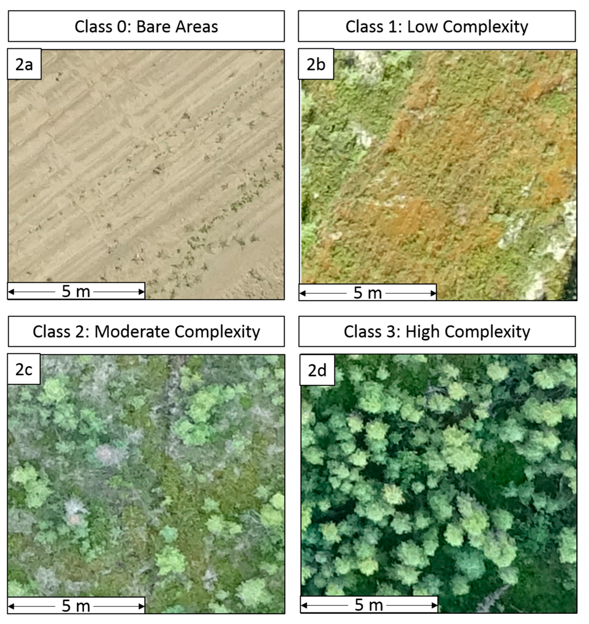
For the purpose of this research, we stratified the study area into four classes of surface complexity, based upon visual observations of the site conditions: tree cover, anticipated surface irregularity (roughness), and visual homogeneity. The four classes were defined as: 0. Bare Areas; 1. Low Complexity; 2. Moderate Complexity; and 3. High Complexity. An example of each class is provided in Figure 2. Class 0 (Figure 2a) exclusively describes the newly constructed roadway and large south pond; Class 1 (Figure 2b) represents linear disturbances within the bog; Class 2 (Figure 2c) includes sparsely treed, undisturbed portions of the bog; and Class 3 (Figure 2d) represents more densely treed areas of undisturbed bog and upland zones.
The spatial distribution of surface complexity classes across the study area is displayed in Figure 1b. The approximate areal coverage of each class is estimated as following: Class 0—5%; Class 1—43%; Class 2—36%; and Class 3—16%. Although, Class 0 areas do not occur in naturally peatland ecosystems, including these points in the assessment serves as a baseline for investigating the effects of surface complexity on point cloud accuracy.
2.2. Data Sets
Two types of data were aquired for this study: terrestrial surveys and remote sensing observations. Descriptions of the assembly and handling of these data are provided in the following sections.
2.2.1. Terrestrial Surveys
Terrestrial ground surveys were used to assess the capacity of remote sensing to characterize terrain within the study area. A total of 678 points were acquired for this purpose, including 474 from cluster sampling and 204 from systematic transects.
Cluster samples were acquired around 48 locations distributed randomly across the study area (Figure 1b). Cluster centers were marked with visible targets that served as ground-control point (GCP) locations for the UAV flights (described below), and so were positioned in locations visible to the sky. As a result, field crews occasionally moved cluster centers up to several meters from their randomly assigned locations. Around each cluster center, field crews surveyed between 6 and 12 points on representative high points (hummocks) and low points (hollows) of terrain, regardless of visibility to the sky.
Additional terrestrial survey points were acquired along three ~10 m transects: two located near the access road and a third in an undisturbed location away from the road (Figure 1b). On these transects, ground elevations were recorded systematically at 10-cm intervals. Visibility to the sky was not a factor in selecting or surveying these transects.
All terrestrial surveys were conducted with a Trimble R4 RTK GNSS system with a base station set up on a nearby survey monument. Average horizontal (x, y) and vertical (z) errors for terrestrial surveys was 0.87 cm and 1.47 cm, respectively.
2.2.2. Remote Sensing Observations
UAV Photogrammetry
Due to persistent full sun conditions, and third-party UAV operator time limitations which prevented early morning or late evening flights, UAV data were collected in two flights on 13 and 14 July, 2016. The first flight was completed in the late afternoon (approximately between 5:00 and 7:00 p.m.) on 13 July and the second in the mid-morning (approximately between 9:00 and 11:00 a.m.) of 14 July. The purpose of conducting two flights was to reduce impacts of deep shadows by collecting complimentary site data with opposing shadow angles, and subsequently using both datasets in point cloud production. Flight data was collected using an Aeryon Scout multirotor platform carrying an HDZoom30 20-megapixel optical camera with global shutter, and approximately 25 min flight duration per battery (3 batteries required to complete flight plan). Moderate average wind speeds were reported for the duration of flight operations (4 m/s on 13 July and 2 m/s on 14 July), and were determined to be acceptable for flight operations as per UAV specifications reported by UAV Geomatics (wind limit of 13.9 m/s) and previous research findings [22,27]. All flights were conducted at 110 m altitude, with a ground-sample distance of 2 cm or less. Parallel flight lines were configured across the site to generate 80% endlap and 60% sidelap amongst individual photos, and photos were obtained in movement (4 m/s flight speed) to minimize the number of required battery replacements.
Ground control was provided by ten permanent GCPs distributed systematically across the study area, and 48 additional GCPs distributed randomly (Figure 1b). As described in Section 2.2.1, these 48 additional GCPs also served as the cluster-center locations for terrestrial surveys. All GCPs were surveyed with the same RTK GNSS system described previously.
Raw UAV photographs were processed using Agisoft PhotoScan [28] to generate a dense point cloud (DPC) and digital orthophotography. In the first step, photo quality was assessed with the Agisoft Photoscan photo-quality assessment tool to determine whether low quality photos (<0.5) existed. From this assessment, all photos were determined to exceed this threshold (reporting > 0.66) and were therefore included in the dataset. Photos were then aligned using camera positions estimated by the onboard GPS during flight, and adjusted with the 10 permanent GCPs in the photos. The sparse point cloud generated through this alignment process was then optimized, with high-error tie points removed, prior to generating a dense point cloud and orthophoto mosaic.
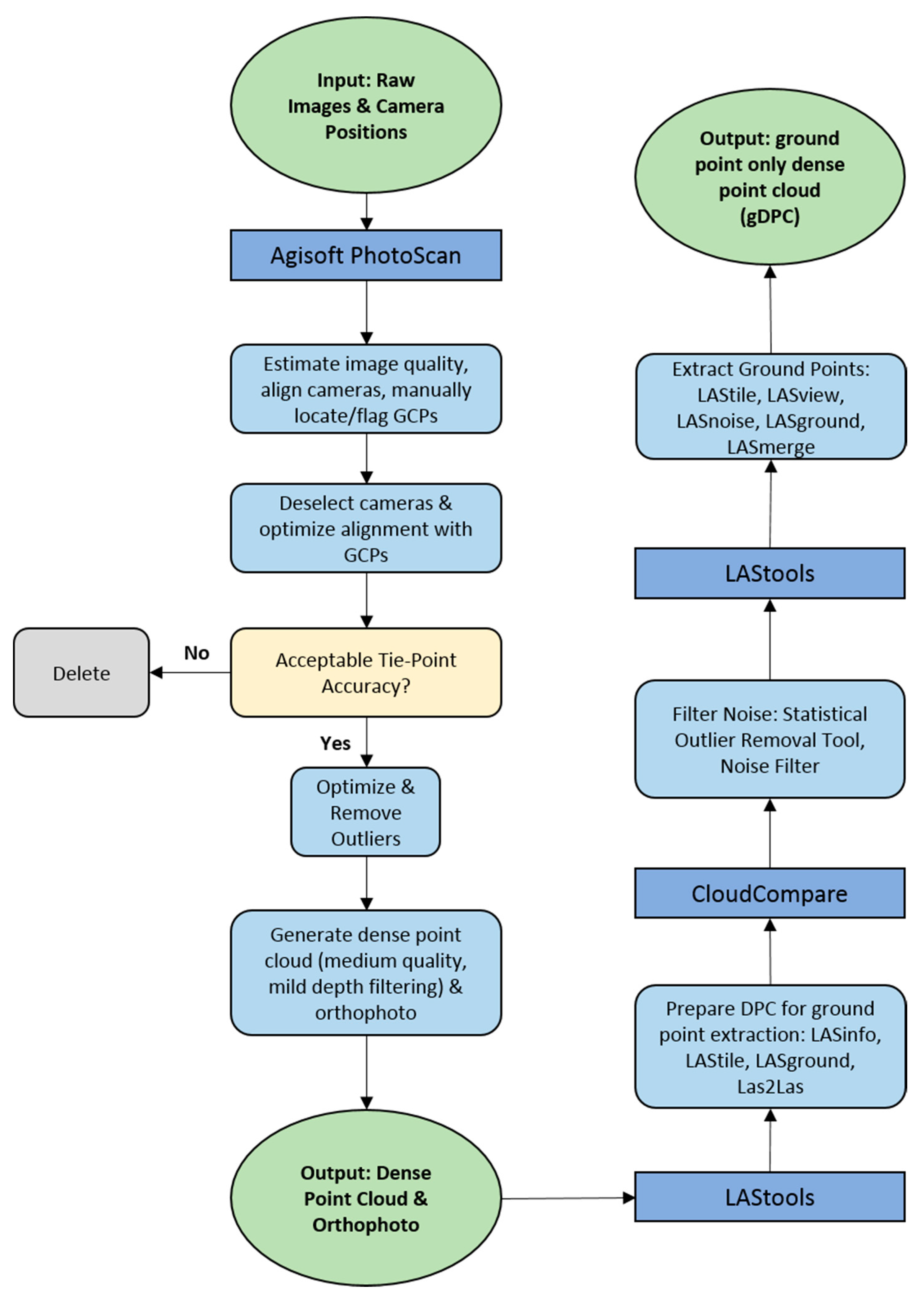
Ground points (i.e., not vegetation) were extracted from the UAV DPC using a combination of LAStools [29] and Cloud Compare [30] software. Cloud Compare is an open-source software package designed specifically for point-cloud processing, and contains significant outlier-removal and noise-filtering tools which we found to work well with photogrammetric data. We used LAStools to perform general tasks such as initial noise filtering, classifying, and merging datasets. This workflow is summarized in Figure 3.
The classified ground DPC (gDPC) was edited manually to remove outliers that had been missed in the automatic filtering process. Point density of the resultant gDPC was calculated at 84.68 pts/m2, although coverage was not uniform across the site and data gaps existed in areas of dense canopy cover. Average point spacing was 13 cm, with a total of 36,880,406 points in the cloud.
LiDAR
LiDAR for the area was commissioned by Shell Canada and collected, processed, and calibrated by Airborne Imaging in May of 2013. This data was provided to the researchers in LAS format for use in this project. Raw point density of this dataset was reported as 4 pts/m2. While we acknowledge the temporal disconnect between the LiDAR data (2013) and those of the UAV and terrestrial surveys (2016), we assume that the terrain elevations, which are the focus of this study, remained constant across this time period.
LAStools was used to classify ground points (ASPRS Class 02) from the raw point cloud (overall classification accuracy 96%), and remove noise from LiDAR data. The point density of the processed data was 2.88 pts/m2, with approximate point spacing of 0.59 m and a total of 1,731,506 points.
Merged UAV Photogrammetry + LiDAR
A combined UAV photogrammetry + LiDAR dataset was generated by merging the UAV gDPC with the ground points classified from LiDAR using LASmerge. While LiDAR clearly had lower overall point densities than the UAV dataset, it was found to have more consistent data coverage across the site, including densely vegetated areas which corresponded with (sometimes large) gaps in the UAV data. Therefore, the purpose of generating this combined dataset was to determine whether point cloud performance could be improved by using the LiDAR to fill these gaps.
2.3. Accuracy Assessments
The capacity of the three remote sensing data sets—(i) UAV photogrammetry; (ii) LiDAR; and (iii) merged UAV photogrammetry + LiDAR—to capture terrain across the study area was asssessed using all appropriate terrestrial-survey points, stratified across the four classes of complexity described in Section 2.1.
2.3.1. UAV Photogrammetry Dataset Performance
A total of 19 GCPs were used to assess the overall accuracy of the dense photogrammetry point cloud (pre-gDPC generation). GCP location and elevation values estimated by PhotoScan were compared with those collected by RTK to determine overall location accuracy (x, y, and z). The comparison of RTK vs reported PhotoScan GCP locations (x, y, z) returned RMSE values of 4 cm, 8 cm, and 13 cm, respectively. These high accuracies were corroborated by mean offset (8 cm) measurements made from the orthophoto.
A rigorous evaluation of terrain accuracy (gDCP) was assessed in two ways; first through comparision of the dataset with all 678 RTK control points, and second by comparing the dataset with with control points stratified by the four classes of surface complexity. Accuracy was determined as the difference between RTK survey point elevations and the nearest point value in the gDCP dataset (gDCP(z) − RTK(z)).
2.3.2. Supplemented LiDAR Performance
The performance of the LiDAR and supplemented UAV photogrammetry+LiDAR datasets were assessed in the same manner as that described for the UAV photogrammetry data (Section 2.3.1 above). Firstly, all suitable RTK points (629 total) were used to assess the overall accuracy, followed by a second assessment of points classified by surface complexity. However, no points were identified in Class 0, since the LiDAR data pre-dated road construction and no alternative bare areas (Class 0) were available. Therefore, we only preformed stratified accuracy assessment for three classes of surface complexity: Low (1); Moderate (2); and High (3).
LiDAR horizontal (x, y) accuracy and vertical (z) accuracy (on flat, hard surfaces) were reported by the acquisition company to be 30 cm and 10 cm, respectively.
2.4. Statistical Analysis
Following the example of previous studies [15,24,31,32], we measured the accuracy and precision of each dataset with root mean squares error (RMSE), average absolute error, mean error, median error, and median offset (the difference between dataset medians).
Since the variance and sample sizes were unequal within the UAV photogrammetry dataset, a robust one-way analysis of variance (ANOVA) and Welch’s test were conducted in SPSS software to determine whether significant differences existed between classes of surface complexity (α = 0.05). Following this, a Tamhane pairwise comparison was conducted to determine where significant differences existed. All results were corroborated by a non-parametric Kruskal-Wallis test.
A two-way mixed model ANOVA test (α = 0.05) was conducted on the UAV Photogrammetry and UAV Photogrammetry + LiDAR datasets in SPSS software to determine whether performance was significantly different between classes and between datasets. Based upon these results, a pairwise comparison was not deemed necessary. A second two-way mixed-model ANOVA test (α = 0.05) was conducted on all three datasets (UAV photogrammetry, LiDAR, and UAV photogrammetry + LiDAR) to determine whether statistically significant differences existed between classes, and between datasets. A subsequent pairwise comparison with a Bonferroni adjustment was used to determine where specific significant differences occurred.
3. Results
Table 1 and Table 2 summarize the results of the elevation accuracy assessments. Table 2 presents dataset performance across all suitable RTK points, while Table 2 shows elevation accuracies of points stratified by surface complexity. There was no statistically significant difference (F(1, 625) = 0.130, p = 0.718) between the overall (unstratified) results obtained by UAV photogrammetry (average absolute error 31 cm, mean error 27 cm, and RMSE 40 cm), and the ‘enhanced’ UAV photogrammetry + LiDAR dataset (average absolute error 30 cm, mean error 27 cm, and RMSE 38 cm). However, LiDAR data alone (average absolute error 42 cm, mean error 41 cm, and RMSE 84 cm) performed significantly worse overall (F(1, 625) = 6.041, p = 0.014). All three data sources displayed positive median offsets: 23 cm for UAV photogrammetry, 27 cm for UAV photogrammetry + LiDAR, and 47 cm for LiDAR alone.
This same relative pattern—no significant difference between UAV photogrammetry alone and UAV photogrammetry + LiDAR (F(2, 625) = 2.292, p = 0.102); significantly worse performance by LiDAR data alone (F(1, 625) = 6.041, p = 0.014) was also observed in the stratified results (Table 2), and we also observed a statistically significant class effect (F(2, 625) = 22.924, p < 0.001). Predictably, errors were found to increase with surface complexity, with the best results found in Class 0 (average absolute error 14 cm, mean error −1 cm, and RMSE 15 cm for UAV photogrammetry), and the worst found in Class 3 (average absolute error 42 cm, mean error 37 cm, and RMSE 51 cm for UAV photogrammetry).
Looking specifically at the UAV photogrammetry data, significant differences could be observed amongst surface-complexity classes (ANOVA: F(3, 674) = 36.969, p < 0.001, Welch: F(3, 134.225) = 53.185, p < 0.001). A post-hoc Tamhane pairwise comparison (α = 0.05) revealed that the performance of these data in Classes 0 and 3 were significantly different from other classes (all p < 0.001), while Classes 1 and 2 performed statistically the same (p = 0.381). A non-parametric Kruskal-Wallis test corroborated these findings.
4. Discussion
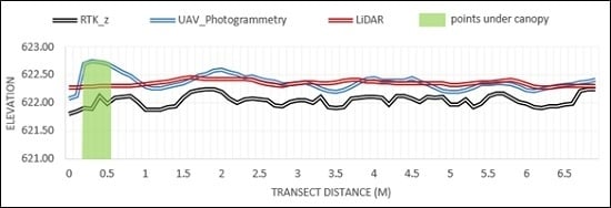
We found UAV photogrammetry to perform better than LiDAR in the task of characterizing terrain across our study site, suggesting that the superior point densities delivered by UAV photogrammetry are more important than the enhanced canopy penetrating abilities of LiDAR. While both technologies tended to over-estimate terrain elevation, we found photogrammetric point clouds to be better able to track microtopographic variability (Figure 4). ‘Enhancing’ photogrammetric datasets with LiDAR does not appear to be worth the increased technical and financial costs.
While the overall errors reported for UAV photogrammetry data (40 cm RMSE) are nominally worse than those reported by other researchers (21 cm from [13]; 4 cm from [15]) we found significant variability amongst surface-complexity classes. Areas of high complexity (Class 3) were found to perform significantly worse than other classes, whose accuracy statistics were more in line with previously published values (Class 0—14 cm; Class 1—21 cm; and Class 2—23 cm). The observation that UAV photogrammetry performed the same across the low and moderate categories of peatland complexity (Classes 1 and 2), suggests that this technology is suitable for characterizing terrain under all but the most-complex conditions. The errors we observed in Class 1 and Class 2 are generally below the scale of microforms (25 cm up to 1 m) across the site, and are therefore likely suitable for mapping microtopography. The fact that highly complex Class 3 areas were relatively rare in our study site—16% of the area as compared to 79% for Classes 1 and 2—lends even further confidence to the notion that UAV photogrammetry can be used to characterize topography in treed bogs such as the one assessed here.
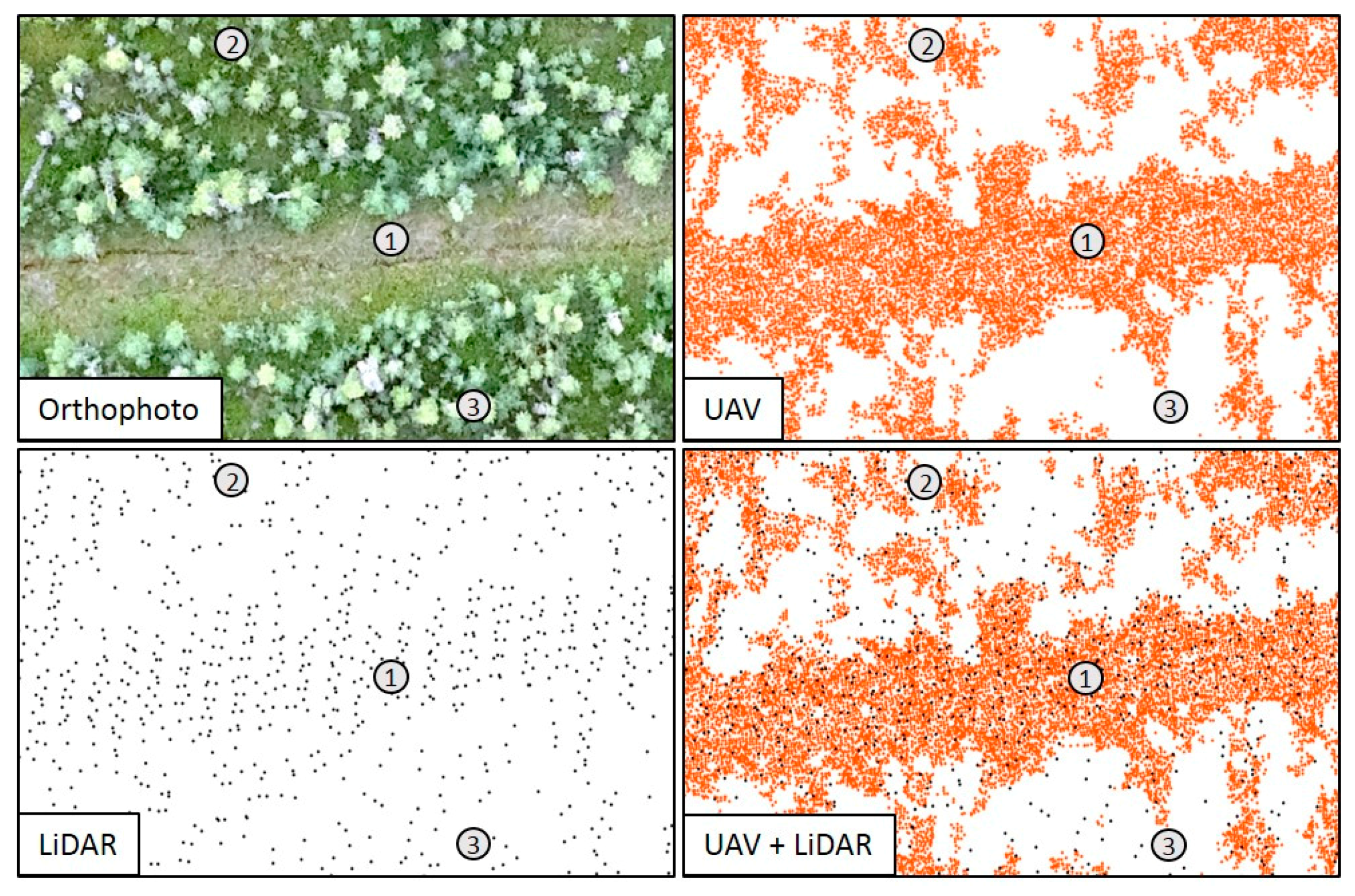
The reduced performance of UAV photogrammetry in highly complex (i.e., heavily treed) areas can be partially explained by the decrease in point density on these sites: 77.5 pts/m2 overall compared to 86.7 pts/m2, 81.3 pts.m2, and 91.6 pts/m2 for Classes 0, 1, and 2, respectively. There are many more ‘data holes’ in these areas as well (Figure 5), reflecting the inability of passive photography to reliably penetrate thick canopies [18]. We had thought that these difficult conditions would be assisted by supplementary LiDAR; this turned out not to be the case in our study site. Not only did UAV photogrammetry + LiDAR fail to perform significantly better than UAV photogrammetry alone in this class (47 cm RMSE vs. 51 cm), but LiDAR data on its own was the worst-performing dataset in Class 3 (58 cm RMSE). While LiDAR is capable of penetrating vegetation canopies to a certain degree, ground point collection is still influenced by vegetation cover [25,33,34], and the point density is far too low overall to accurately capture microtopographic variability (Figure 5).
While UAV photogrammetry alone is capable of mapping most treed-bog terrain at acceptable levels of accuracy, its spatial coverage is limited: typically less than 100 ha for UAV platforms, which must fly within visible line of sight. While airborne LiDAR can cover larger areas, it is more expensive to fly, and typically not acquired at point densities sufficient for mapping peatland microtopography. We did not test high-density LiDAR, but our observations suggest that densities would have to exceed 30–50 pts/m2 in order to be effective at this task.
Potential Sources of Error
All data used in this research are subject to a variety of error sources during collection, processing, and analysis. Firstly, the RTK GNSS system is subject to errors introduced by satellite and radio link connectivity, which is reliant upon external factors such as canopy cover [13], and differences in measurement techniques between field personnel. In order to mitigate these errors, survey summaries were reviewed to ensure RTK points used in the comparisons were reported at accuracies reasonable for microform scale (<20 cm). Additionally, we maintained consistency in field personnel to reduce errors in ground measurements.
UAV photogrammetry data may be compromised by external factors such as flight and weather conditions. To offset these sources of error, multiple flights were conducted to address deep shadows resulting from full sun conditions, as described in Section 2.2.1. Additionally, flights were completed in low to moderate wind (<4 m/s) and dry conditions (little to no standing water and/or moisture present at surface in vegetated areas) to reduce errors associated with these factors. Standing water was observed along the newly constructed roadway, which may have increased errors associated with Class 0 areas. However, as Class 0 areas do not occur naturally within peatland ecosystems, correcting for this source of error was not deemed a priority. Increased overlap may have improved overall model accuracies in areas of highly complex terrain, and should be considered in similar future studies. The distribution and number of GCPs was determined to be adequate for the study area, and not a major anticipated source of error, as ten GCPs per km2 is a well-established standard in aerial photogrammetry [35,36].
5. Conclusions
The primary objective of this research was to evaluate the capacity of UAV photogrammetry to characterize terrain elevation in a boreal treed bog across four categories of vegetation/surface complexity: bare, low, medium, and high. Photogrammetric data were found to perform well under all but the worst (heavily treed) conditions, with RMSE accuracies ranging from 14–23 cm. Based on this assessment, we suggest that UAV photogrammetric technology provides a reasonable foundation for supplementing or even replacing traditional RTK GNSS ground surveys for characterizing peatland terrain in low- and moderately complex conditions. While positive elevation offsets can be expected to occur, the high point density provided by this technology is generally capable of tracking microtopographic terrain undulations. This capacity can be expected to diminish (we documented 42 cm RMSE) in areas of high surface complexity due to the inability of passive photography to reliably penetrate thick vegetation canopies. As a result, site conditions should be considered carefully prior to adopting this technology in peatland-terrain-mapping applications, and researchers should determine whether or not the anticipated accuracies will meet the intended purpose.
We also assessed the value of supplementary LiDAR over the same gradient of complexity, anticipating that the enhanced canopy penetrating capacity of this technology might work well with the enhanced point densities provided by photogrammetry. However, we found no support for this concept, suggesting the type of low-density (ours was 2.88 pts/m2) LiDAR data typically available to researchers is not worth the increased technical and financial costs.
Peatlands are highly diverse, and we would encourage additional studies aimed at characterizing terrain at other study areas, and under different conditions. In particular, it would be interesting to assess the impact of phenological condition (leaf-on, leaf-off), shadow, and atmospheric effects on UAV photogrammetry. The capacity of the technology seems tightly tied to the ability to photograph the ground reliably. Moving from general terrain characterization (spot elevations) to true microtopographic mapping (classifying hummocks and hollows) is another logical next step.
Acknowledgments
Research funding was provided by Emissions Reduction Alberta (Grant # BI40020) and Shell Canada Ltd. We also thank Shell Canada for site access and logistical support, NAIT and the University of Waterloo for assisting with project design and facilitating field data collection, and Tak Fung with the University of Calgary for his assistance with data analysis.
Author Contributions
J.L., M.M.R., and G.J.M. conceived the study and wrote the paper. J.L. and M.M.R. analyzed the data. G.J.M contributed resources and field equipment.
Conflicts of Interest
The authors declare no conflict of interest. The founding sponsors had no role in the design of the study; in the collection, analyses, or interpretation of data; in the writing of the manuscript, and in the decision to publish the results.
References
- Lucieer, A.; Robinson, S.A.; Bergstrom, B. Aerial ‘OktoKopter’ to map Antarctic moss. Aust. Antarct. Mag. 2010, 19, 1–13. [Google Scholar]
- Couwenberg, J.; Thiele, A.; Tanneberger, F.; Augustin, J.; Bärisch, S.; Dubovik, D.; Liashchynskaya, N.; Michaelis, D.; Minke, M.; Skuratovich, A.; et al. Assessing greenhouse gas emissions from peatlands using vegetation as a proxy. Hydrobiologia 2011, 674, 67–89. [Google Scholar] [CrossRef]
- Macrae, M.L.; Devito, K.J.; Strack, M.; Waddington, J.M. Effect of water table drawdown on peatland nutrient dynamics: Implications for climate change. Biogeochemistry 2013, 112, 661–676. [Google Scholar] [CrossRef]
- Comas, X.; Kettridge, N.; Binley, A.; Slater, L.; Parsekian, A.; Baird, A.J.; Strack, M.; Waddington, J.M. The effect of peat structure on the spatial distribution of biogenic gases within bogs. Hydrol. Process. 2014, 28, 5483–5494. [Google Scholar] [CrossRef]
- Food and Agriculture Organization of the United Nations (FAO). Towards Climate-Responsible Peatlands Management. 2014. Available online: http://www.fao.org/3/a-i4029e.pdf (accessed on 3 February 2016).
- Cresto Aleina, F.; Runkle, R.K.; Kleinen, T.; Kutzbach, L.; Schneider, J.; Brovkin, V. Modeling micro-topographic controls on boreal peatland hydrology and methane fluxes. Biogeosciences 2015, 12, 5689–5704. [Google Scholar] [CrossRef]
- Acharya, S.; Kaplan, D.A.; Casey, S.; Cohen, M.J.; Jawitz, J.W. Coupled local facilitation and global hydrologic inhibition drive landscape geometry in a patterned peatland. Hydrol. Earth Syst. Sci. 2015, 19, 2133–2144. [Google Scholar] [CrossRef]
- Strack, M.; Waddington, J.M.; Rochefort, L.; Tuitilla, E.S. Response of vegetation and net ecosystem carbon dioxide exchange at different peatland microforms following water table drawdown. J. Geophys. Res. 2006, 111, 1–10. [Google Scholar] [CrossRef]
- Farmer, J.; Matthews, R.; Smith, J.U.; Smith, P.; Singh, B.K. Assessing existing peatland models for their applicability for modelling greenhouse gas emissions from tropical peat soils. Curr. Opin. Enviorn. Sustain. 2011, 3, 339–349. [Google Scholar] [CrossRef]
- Shi, X.; Thornton, P.W.; Ricciuto, D.M.; Hanson, P.J.; Sebestyen, S.D.; Griffiths, N.A.; Bisht, G. Representing northern peatland microtopography and hydrology within the Community Land Model. Biogeosciences 2015, 12, 6463–6477. [Google Scholar] [CrossRef]
- Lehmann, J.R.K.; Munchberger, W.; Knoth, C.; Blodau, C.; Nieberding, F.; Prinz, T.; Pancotto, V.A.; Kleinebecker, T. High-Resolution Classification of South Patagonian Peat Bog Microforms Reveals Potential Gaps in Up-Scaled CH4 Fluxes by use of Unmanned Aerial System (UAS) and CIR Imagery. Remote Sens. 2016, 8, 1–19. [Google Scholar] [CrossRef]
- Pouliot, R.; Rochefort, L.; Karofeld, E. Initiation of microtopography in revegetated cutover peatlands. Appl. Veg. Sci. 2011, 14, 158–171. [Google Scholar] [CrossRef]
- Roosevelt, C. Mapping site site-level microtopography with Real-Time Kinematic Global Navigation Satellite Systems (RTK GNSS) and Unmanned Aerial Vehicle Photogrammetry (UAVP). Open Archaeol. 2014, 2014, 29–53. [Google Scholar] [CrossRef]
- Sturm, P.; Triggs, B. A factorization based algorithm for multi-image projective structure and motion. In Proceedings of the 4th European Conference on Computer Vision, Cambridge, UK, 15–18 April 1996. [Google Scholar]
- Lucieer, A.; Turner, D.; King, D.H.; Robinson, S.A. Using an Unmanned Aerial Vehicle (UAV) to capture micro-topography of Antarctic moss beds. Int. J. Appl. Earth Obs. Geoinf. 2014, 27, 53–62. [Google Scholar] [CrossRef]
- Strack, M. (Ed.) Peatlands and Climate Change; International Peat Society (IPS): Saarijärvi, Finland, 2008. [Google Scholar]
- Munir, T.M.; Xu, B.; Perkins, M.; Strack, M. Responses of carbon dioxide flux and plant biomass to water table drawdown in a treed peatland in northern Alberta: a climate change perspective. Biogeosciences 2014, 11, 807–820. [Google Scholar] [CrossRef]
- Javernick, L.; Brasington, J.; Caruso, B. Modeling the topography of shallow braided rivers using Structure-from-Motion photogrammetry. Geomorphology 2014, 213, 166–182. [Google Scholar] [CrossRef]
- Jensen, J.; Mathews, A. Assessment of Image-Based Point Cloud Products to Generate a Bare Earth Surface and Estimate Canopy Heights in a Woodland Ecosystem. Remote Sens. 2016, 8, 50. [Google Scholar] [CrossRef]
- Zainuddin, K.; Jaffri, M.; Zainal, M.; Ghazali, N. Verification Test on Ability to Use Low-Cost UAV for Quantifying Tree Height. In Proceedings of the IEEE 12th International Colloquium on Signal Processing & Its Applications, Melaka, Malaysia, 4–6 March 2016. [Google Scholar]
- Mancini, F.; Dubbini, M.; Gattelli, M.; Stecchi, F.; Fabbri, S.; Gabbianelli, G. Using Unmanned Aerial Vehicles (UAV) for High-Resolution Reconstruction of Topography: The Structure from Motion Approach on Coastal Environments. Remote Sens. 2013, 5, 6880–6898. [Google Scholar] [CrossRef]
- Rosnell, T.; Honkavaara, E. Point Cloud Generation from Aerial Image Data Acquired by a Quadrocopter Type Micro Unmanned Aerial Vehicle and a Digital Still Camera. Sensors 2012, 12, 453–480. [Google Scholar] [CrossRef] [PubMed]
- James, M.; Robson, S. Straightforward reconstruction of 3D surfaces and topography with a camera: Accuracy and geoscience application. J. Geophys. Res. 2012, 117. [Google Scholar] [CrossRef]
- Harwin, S.; Lucieer, A. Assessing the Accuracy of Georeferenced Point Clouds Produced via Multi-View Stereopsis from Unmanned Aerial Vehicle (UAV) Imagery. Remote Sens. 2012, 4, 1573–1599. [Google Scholar] [CrossRef]
- Lefsky, M.A.; Cohen, W.B.; Parker, G.G.; Harding, D.J. Lidar remote sensing for ecosystem studies: Lidar, an emerging remote sensing technology that directly measures the three-dimensional distribution of plant canopies, can accurately estimate vegetation structural attributes and should be of particular interest to forest, landscape, and global ecologists. BioScience 2002, 52, 19–30. [Google Scholar]
- Pirotti, F.; Tarolli, P. Suitability of LiDAR point density and derived landform curvature maps for channel network extraction. Hydrol. Process. 2010, 24, 1187–1197. [Google Scholar] [CrossRef]
- UAV Geomatics. Aeryon Scout Technical Specifications. 2011. Available online: http://www.uavgeomatics.com/services/system/scout.pdf (accessed on 12 June 2017).
- AgiSoft PhotoScan Professional Edition (Version 1.2.4) [Software]. 2016. Available online: http://www.agisoft.com/downloads/installer/ (accessed on 3 June 2016).
- Isenburg, M. LAStools—Efficient LiDAR Processing Software (Version 160110, Licensed) [Software]. 2016. Available online: http://rapidlasso.com/LAStools/ (accessed on 3 June 2016).
- CloudCompare (Version 2.7.0) [GPL Software]. 2016. Available online: http://www.cloudcompare.org/ (accessed on 8 August 2016).
- Turner, D.; Lucieer, A.; Watson, C. An Automated Technique for Generating Georectified Mosaics from Ultra-High Resolution Unmanned Aerial Vehicle (UAV) Imagery, Based on Structure from Motion (SfM) Point Clouds. Remote Sens. 2012, 4, 1392–1410. [Google Scholar] [CrossRef]
- Mercer, J.; Westbrook, C. Ultrahigh-resolution mapping of peatland microform using ground-based structure from motion with multiview stereo. Biogeosciences 2016, 121, 2901–2916. [Google Scholar] [CrossRef]
- Hopkinson, C.; Chasmer, L.; Sass, G.; Creed, I.F.; Sitar, M.; Kalbfleisch, W.; Treitz, P. Vegetation class dependent errors in Lidar ground elevation and canopy height estimates in a boreal wetland environment. Can. J. Remote Sens. 2005, 31, 191–206. [Google Scholar] [CrossRef]
- Chasmer, L.; Hopkinson, C.; Treitz, P. Investigating laser pulse penetration through a conifer canopy by integrating airborne and terrestrial lidar. Can. J. Remote Sens. 2006, 32, 116–125. [Google Scholar] [CrossRef]
- Krauss, K. Photogrammetry, Volume 2: Advanced Methods and Applications, 4th ed.; Dümmler: Bonn, Germany, 1997. [Google Scholar]
- McGlone, C.; Mikhail, E.; Bethel, J. Manual of Photogrammetry, 5th ed.; ASPRS: Bethesda, MD, USA, 2004. [Google Scholar]
Figure 1.
Approximate site location in the province of Alberta (AB) with reference to nearby notable city centers (1a); Estimated distribution of surface complexity classes across the study site (1b). An extensive network of linear disturbances transect the site. Areas between these features are assumed to be undisturbed and indicative of natural boreal treed bog conditions within the region. GCP installation locations, cluster sample and detailed transect points are shown (1b), and described in Section 2.2.1.

Figure 2.
Examples of each surface complexity class found within the study site. Data displayed is captured from the orthophoto. The example of Class 0 (2a) is taken from the new clay road bisecting the study area, Class 1 (2b) is taken from a pipeline ROW, Class 2 (2c) is from undisturbed portions of the bog, and Class 3 (2d) is from densely treed portion of bog.

Figure 3.
Photogrammetric and point-cloud management software workflow illustrating the process of using UAV flight data to generate secondary (DPC and orthomosaic) and tertiary products (ground dense point cloud (gDPC)) used in this research.
Figure 3.
Photogrammetric and point-cloud management software workflow illustrating the process of using UAV flight data to generate secondary (DPC and orthomosaic) and tertiary products (ground dense point cloud (gDPC)) used in this research.

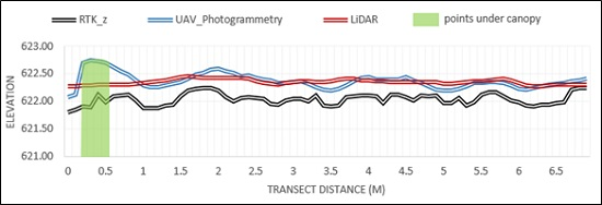
Figure 4.
A comparison of dataset performance along a detailed transect within an undisturbed portion of the study site (representing a mixture of Classes 2 and 3). Both UAV photogrammetry and LiDAR overestimate ‘true’ ground-surface elevation, represented in black, though UAV photogrammetry is better-able to capture microtopographic variability. The area in green indicates ground points that were fully covered by vegetation canopy.
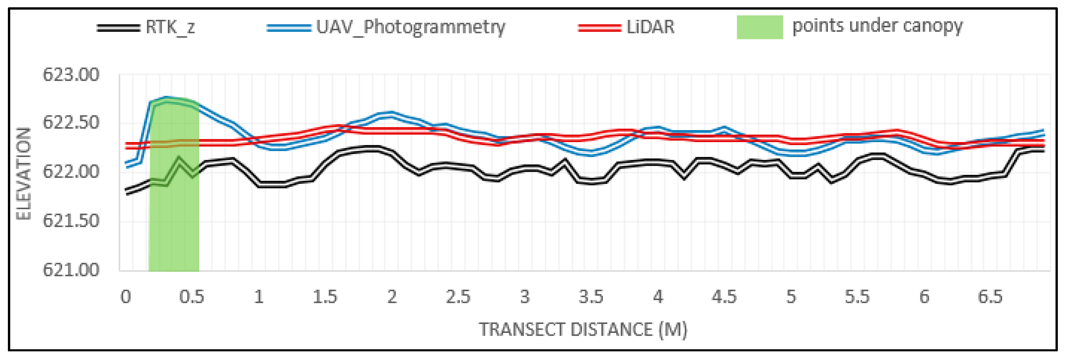
Figure 5.
Comparison of vegetation influence on dataset point densities, modeling a seismic line and adjacent undisturbed peatland. Examples of each surface complexity class indicated as: ① = Class 1 (low); ② = Class 2 (moderate); ③ = Class 3 (high).
Figure 5.
Comparison of vegetation influence on dataset point densities, modeling a seismic line and adjacent undisturbed peatland. Examples of each surface complexity class indicated as: ① = Class 1 (low); ② = Class 2 (moderate); ③ = Class 3 (high).


Table 1.
Dataset Accuracies: Comparison of Dataset Elevations against all RTK Surveyed Point Elevations (678 UAV Photogrammetry dataset and 629 LiDAR and UAV photogrammetry + LiDAR datasets).
Table 1.
Dataset Accuracies: Comparison of Dataset Elevations against all RTK Surveyed Point Elevations (678 UAV Photogrammetry dataset and 629 LiDAR and UAV photogrammetry + LiDAR datasets).
| Dataset | Average Absolute z Error (cm) | Mean z Error (cm) | RMSE (cm) | Median z Error (cm) | Median z Offset (cm) |
|---|---|---|---|---|---|
| UAV Photogrammetry | 31 | 27 | 40 | 25 | 23 |
| LiDAR | 42 | 41 | 84 | 25 | 47 |
| UAV Photogrammetry + LiDAR | 30 | 27 | 38 | 25 | 27 |
Table 2.
Dataset Accuracies: Comparison of Dataset Elevations against RTK Point Elevations Classified by Surface Complexity.
Table 2.
Dataset Accuracies: Comparison of Dataset Elevations against RTK Point Elevations Classified by Surface Complexity.
| Class | Dataset | Average ABS z Error (cm) | Mean Error (cm) | RMSE (cm) | Median z Error (cm) | Median z Offset (cm) |
|---|---|---|---|---|---|---|
| Class 0 | UAV | 14 | −1 | 15 | −8 | −10 |
| (42 points) | ||||||
| Class 1 | UAV | 21 | 15 | 26 | 15 | −10 |
| LiDAR | 14 | 12 | 18 | 10 | −1 | |
| (53 points) | UAV + LiDAR | 20 | 14 | 25 | 14 | −6 |
| Class 2 | UAV | 23 | 21 | 28 | 20 | 15 |
| LiDAR | 34 | 33 | 68 | 23 | 33 | |
| (264 points) | UAV + LiDAR | 23 | 21 | 27 | 20 | 15 |
| Class 3 | UAV | 42 | 37 | 51 | 35 | 47 |
| LiDAR | 58 | 56 | 110 | 29 | 56 | |
| (312 points) | UAV + LiDAR | 39 | 35 | 47 | 32 | 46 |
© 2017 by the authors. Licensee MDPI, Basel, Switzerland. This article is an open access article distributed under the terms and conditions of the Creative Commons Attribution (CC BY) license (http://creativecommons.org/licenses/by/4.0/).
Share and Cite
MDPI and ACS Style
Lovitt, J.; Rahman, M.M.; McDermid, G.J. Assessing the Value of UAV Photogrammetry for Characterizing Terrain in Complex Peatlands. Remote Sens. 2017, 9, 715. https://doi.org/10.3390/rs9070715
AMA Style
Lovitt J, Rahman MM, McDermid GJ. Assessing the Value of UAV Photogrammetry for Characterizing Terrain in Complex Peatlands. Remote Sensing. 2017; 9(7):715. https://doi.org/10.3390/rs9070715
Chicago/Turabian StyleLovitt, Julie, Mir Mustafizur Rahman, and Gregory J. McDermid. 2017. "Assessing the Value of UAV Photogrammetry for Characterizing Terrain in Complex Peatlands" Remote Sensing 9, no. 7: 715. https://doi.org/10.3390/rs9070715
Note that from the first issue of 2016, this journal uses article numbers instead of page numbers. See further details here.