Stem Measurements and Taper Modeling Using Photogrammetric Point Clouds


College of Forestry, Oregon State University, 3100 Jefferson Way, Corvallis, OR 97333, USA
*
Author to whom correspondence should be addressed.
Remote Sens. 2017, 9(7), 716; https://doi.org/10.3390/rs9070716
Submission received: 3 May 2017
/
Revised: 7 July 2017
/
Accepted: 9 July 2017
/
Published: 12 July 2017
(This article belongs to the Section Forest Remote Sensing)
Abstract
:The estimation of tree biomass and the products that can be obtained from a tree stem have focused forest research for more than two centuries. Traditionally, measurements of the entire tree bole were expensive or inaccurate, even when sophisticated remote sensing techniques were used. We propose a fast and accurate procedure for measuring diameters along the merchantable portion of the stem at any given height. The procedure uses unreferenced photos captured with a consumer grade camera. A photogrammetric point cloud (PPC) is produced from the acquired images using structure from motion, which is a computer vision range imaging technique. A set of 18 loblolly pines (Pinus taeda Lindl.) from east Louisiana, USA, were photographed, subsequently cut, and the diameter measured every meter. The same diameters were measured on the point cloud with AutoCAD Civil3D. The ground point cloud reconstruction provided useful information for at most 13 m along the stem. The PPC measurements are biased, overestimating real diameters by 17.2 mm, but with a reduced standard deviation (8.2%). A linear equation with parameters of the error at a diameter at breast height (d1.3) and the error of photogrammetric rendering reduced the bias to 1.4 mm. The usability of the PPC measurements in taper modeling was assessed with four models: Max and Burkhart [1], Baldwin and Feduccia [2], Lenhart et al. [3], and Kozak [4]. The evaluation revealed that the data fit well with all the models (R2 ≥ 0.97), with the Kozak and the Baldwin and Feduccia performing the best. The results support the replacement of taper with PPC, as faster, and more accurate and precise product estimations are expected.
1. Introduction
Forest inventory is focused on the estimation of existing resources with techniques that are simultaneously fast, accurate, precise, and cost effective [5,6,7]. Ground estimates are enhanced by remote sensing techniques, particularly lidar, which provide a wealth of data at reduced costs [8,9]. However, looking at the forest from above limits access to valuable information with respect to product identification from individual trees. Regardless of the sensor (i.e., active or passive), a nadir view fails to capture relevant information about the stem. Therefore, either ground inventory focused on stem product is executed or taper models are used to predict the products that can be obtained from each stem. In practical applications, a stem is described from ground measurements with two procedures: one based on measuring the diameter at various heights with optical devices [10,11,12,13], and one based on point clouds, such as terrestrial laser scanning [14,15,16,17]. Both approaches are time-consuming and not necessarily unexpensive. Besides the significant time needed to acquire the information, accuracy issues are present. Optical devices overestimate the actual diameter by more than 1 mm on average, which could seem insignificant. However, the standard deviation is at least 10 times larger than the mean [10], which suggests that the quality of the measurements depends on the operator as much as on the method or device. An overestimation of the diameter also occurs when lidar serves as the input, depending on the approach, by as much as 25 mm [17]. Compared with ground measurements, taper models require a significant development effort, but once completed the only information needed to estimate product allocation along a stem is the diameter at breast height (d1.3) and total height [18]. However, mixed results were obtained when a taper was used in product identification and estimation, some arguing for [19], and some against [20,21].
An alternative to time-consuming (i.e., ground measurements) or expensive point clouds (i.e., terrestrial lidar) is a reconstruction of reality with computer vision techniques. The main product of computer vision procedures is a point cloud built from two-dimensional (2D) images [22,23]. The distinction between the computer vision-based point clouds and the clouds produced from stereo images is the reduced importance, up to elimination, of the stereometric information in the former. The creation of point clouds with stereopsis is possible, but is slow, difficult to implement in the field, and requires significant post-processing. Image processing is implemented in many instances with expensive software, such as ENVI [24] or IMAGINE Photogrammetry (former Leica Photogrammetry Suite) [25]. The need for performant software is rooted in stereopsis (i.e., it operates with one pair of images at a time), which supplies only a partial view of the trees. To render the entire tree, multiple image acquisition positions are needed, each location producing point clouds that have to be merged subsequently. Therefore, stereometric techniques focused on three-dimensional (3D) rendering are not considered operationally feasible for activities occurring under a forest canopy. The lack of stereometry labels the computer vision derived points as photogrammetric [26,27]. The representation of reality with 3D points is not new [28,29], but gained momentum in forestry when commercial applications became available, such as Agisoft [30], Pix4D [31], or VisualSFM [32]. A large number of papers using photogrammetric point clouds (PPC) describe the forest from above, similarly to aerial lidar [33]. However, the presence of a passive sensor limits the ability of PPC to reach the ground; therefore, they were used either in combination with other data (such as digital terrain models) or confined to the upper canopy. Currently, researchers investigate the applicability of the structure from motion (SfM) technique, a computer vision procedure, in reconstructing the lower portion of a tree stem [34,35]. Success was noticed in the estimation of d1.3, in many instances with precision superior to terrestrial lidar [34]. The encouraging SfM results recommended an expansion from d1.3 to the diameter along the stem. Therefore, the objective of this research is an assessment of the accuracy of diameter measurements executed from the PPC obtained with the SfM technique. A secondary objective is a comparison between the diameters measured from PPC and the diameters estimated from taper equations.
2. Methods
2.1. Field Data Collection
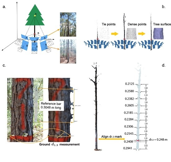
The accuracy and precision of the diameter measurements executed on PPC was assessed using 18 loblolly pines (Pinus taeda Lindl.) from west central Louisiana (Figure 1a,b). The trees were chosen to describe stands that are ready for a silvicultural prescription (Figure 1c) (i.e., a thinning or regeneration harvest), and mirror other studies focused on taper modeling [36,37,38]. The selected trees were positioned in the dominant and codominant crown classes, which according to Nyland [39] receive unobstructed light from above and at least one side (Figure 1d). Trees located in the upper crown classes (i.e., dominant and codominant) are the focus of active forest management, as they are not only the most valuable trees but also the ones that define the forest stand, and consequently, the ecosystem’s dynamics [40]. The trees were scheduled for either the first thin (i.e., mechanical thinning) or for final cut (i.e., clearcut). The average d1.3 was on average 306.1 mm (variance 68.5), ranging from 213.0 mm to 449.6 mm. The total height (H) varied from 15.9 m to 26.8 m, with an average of 22.2 m and a variance of 12.8. The trees grew on productive sites, with site indices ≥60 at base age 25. Each tree was photographed with a Nikon D3200 (i.e., a complementary metal–oxide–semiconductor sensor of 23.2 mm × 15.4 mm) equipped with a Nikkor AF-S DX VR 18–55 mm zoom lens (aperture 3.5–5.6). To capture as much as possible from the tree, the images were acquired at the focal length of 18 mm. For calibration, each tree had the d1.3 painted circularly, and on opposite sides of the d1.3 two metal rods of 304.8 mm (i.e., 1 foot) were freely hanged. Shortly after the images were captured, the trees were felled and the diameter along the stem was measured every meter with a Spencer D-tape starting from d1.3, which was marked at 1.3 m. The accuracy of measurements was 1 mm for diameters and 10 mm for lengths along the stem (i.e., height). To verify the total length after the tree was felled, the total height was extracted from lidar data. The lidar flight scanning the area was executed in March 2012, at most four months before the trees were photographed and cut. To accommodate for the growth between flight time and field measurements, we considered that trees could have increased their height with at most 1 m. The point density was on average 30 points/m2.
2.2. Photorammetric Point Cloud Generation and Diameter Measurements
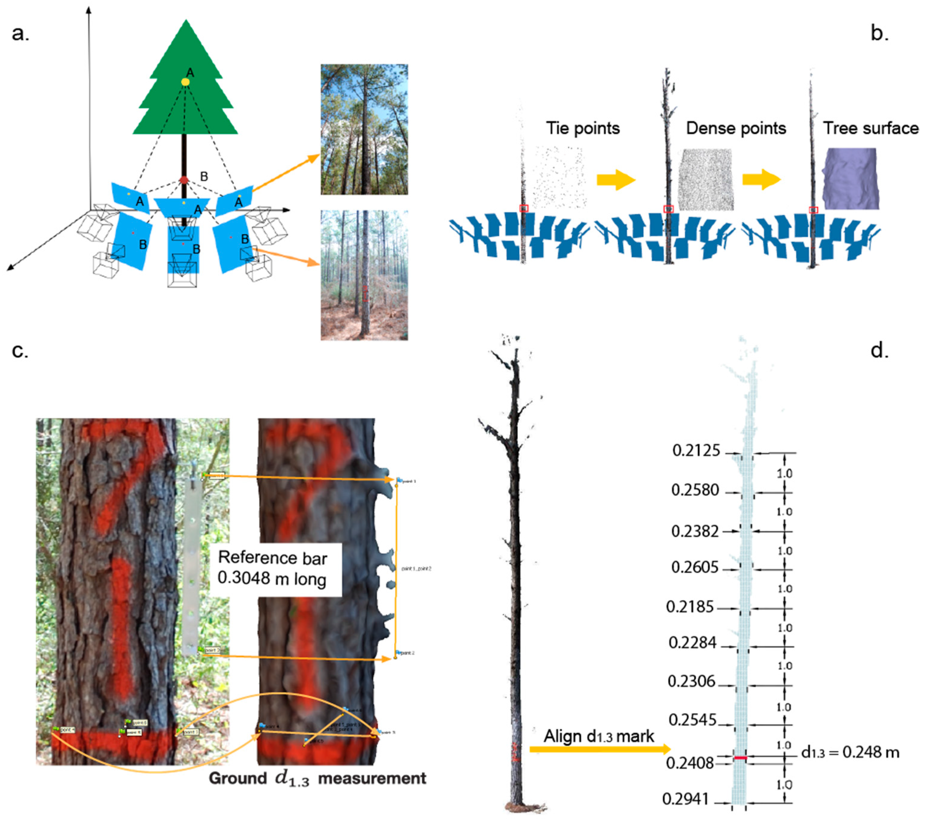
The PPC were generated using SfM implemented in Agisoft PhotoScan ver 1.2 [30]. Tree reconstruction and stem diameter measurements from the PPC were executed in four steps (Figure 2a–d): (1) photo alignment, (2) build the point cloud, (3) scale the point cloud, and (4) measure diameter along the stem. The crucial step of SfM is concerned with the alignment of images, which if not completed properly will render an unusable PPC. Depending on computational power (i.e., the microprocessor), the amount of detail existing inside the image (i.e., the number of pixels), and the time available for processing the alignment can be executed in a few seconds or a few hours. In Agisoft, there are four parameters determining the time and quality of photo alignment: accuracy of camera position, matching detected features across images, the number of key points (i.e., image specific feature points that can represent same entities in multiple images), and tie points (i.e., image specific points used for matching images). Accurate camera locations are obtained when original images are used unaltered, which in Agisoft is coded as “high” [41]. However, this option is time-consuming; therefore, a lower accuracy can be used [42], such as medium, which downscales each side of the image by a factor of 2. Liang et al. [42] obtained good results by a low alignment of photos with a resolution of 5472 × 3648 pixels, which employed only of the information recorded (i.e., 1368 × 912). In our study, the image resolution was 3872 × 2592 pixels, and we aligned the photos by downscaling the original images by half (i.e., 1936 × 1296). Through experimentation, the maximum number of key points was set to 100,000 and the number of tie-points to 60,000.
Photos were captured around the trees in pairs to cover the lower and higher portions of the stem (Figure 2a). Each pair overlapped ≥50%, to ensure sufficient common features for successful photo alignment. Georeference provides auxiliary information that helps camera positioning. However, by operating below the canopy no reliable GPS coordinates were acquired; therefore, the photos were aligned by relying only on the presence of the same features on multiple images. At least 10,000 tie-points/image were used for photo alignment and camera positioning.
The second step occurs after photos alignment, and consists in a densification of the tie-points (Figure 2b). For each tree, the final PPC was created by downscaling the images by a factor of 2, which produced enough points for precise measurements without sacrificing processing time. All trees were described with a PPC of at least 600,000 points (the maximum was approximately 2 million), at least 25,000 points/m2. To ensure precise measurements, we reconstructed the surface of the trunk with at least 500,000 faces (Figure 2b). The faces were built with a ratio of 1:5 to the number of points. Compared with previous studies of image-based forest inventories [34,35,42], the selected parameters for SfM in Agisoft (Table 1) were either similar or provided superior solutions.
Because the images were not georeferenced and no ground control points were present, the PPC is in relative and not absolute units. Therefore, to measure diameters, the PPC and the associated surface had to be scaled. To minimize the errors, scaling was implemented using measurements executed on two perpendicular planes. On the horizontal plane, the ground measured d1.3 was assigned to the corresponding segment from the PPC. The scale on the vertical plane was carried out by allocating the known length of the metal bar (i.e., 304.8 mm) to the distance between the points delineating the bar inside the PPC (Figure 2c). After the length of the metal bar was introduced, the d1.3 on two approximately perpendicular diameters was entered. Based on the tree values, Agisoft computes the scaling error by subtracting the estimated value from the inputted value [30]. If the scaling error was larger than 5% of the field measured d1.3, then the two diameters were re-measured on different positions. Depending on the size of the tree, the root mean square of the error ranged from 6.9 mm to 22.1 mm. Considering that the relationship among points inside the PPC are correct (i.e., are similar to reality) and unchanged, the maximum error that is expected for any linear measurement is 22.1 mm. Scaling is one of the three main sources of errors when PPC are used for actual measurements, and usually increases the magnitude of the investigated attributes with at least one order of magnitude (in our case three orders, from 1 to 1000).
Current guidelines consider field measurements accurate if the difference between the actual and measured d1.3 is <5% [43]. The average d1.3 measured in the field is 306 mm. Because the calibrating metal bar was 304.8 mm (i.e., close to the d1.3 of measured trees), we considered that a vertical error of 5% is also admissible, even when field measurements for heights accept errors of <10% [43]. Therefore, the accepted total error for accurate field measurements is 21.6 mm (i.e., ). For consistency, a similar value could have been used for PPC accuracy, but we decided to tighten the requirements. Consequently, we considered that scaling will have a limited impact on measurements if the total error (i.e., horizontal and vertical) is <10 mm (less than half of the field accepted accuracy).
The last step consists in measuring the diameters every meter along the stem (Figure 2d), which was executed in AutoCAD Civil 3D [44]. The second source of PPC measurement error is matching the ground diameters with PPC-estimated diameters. The matching can be implemented in two ways: (1) identify d1.3 as the middle of the colored band marking the d1.3 in the PPC, then measure all diameters starting from the identified d1.3 (i.e., 1.3 m), or (2) identify the ground in the PPC, then measure the diameters with respect to the ground. Both ways offer a check, as either the ground should be at a height (length) of 0 (i.e., former), or d1.3 should fall inside the colored band (i.e., later). Even when the difference between the d1.3 identified using the two ways should be minor, its propagation could have a significant impact, particularly for the upper section of the stem. Therefore, diameters were measured in both ways.
In AutoCAD, the diameters were measured on a plane perpendicular to the axis of the tree. The diameters were measured in two ways: one mirroring the field procedures for taper estimation from the ground (i.e., side view of the stem), and one mirroring the approach of You et al. [16] (i.e., top view or circumference-based). The side measurement was acquired by averaging four diameters obtained by rotating the stem by approximately 90°. The circumferential measurement was obtained in four steps: (1) section the stem at levels corresponding to the ground measured diameters, (2) eliminate branches and knots, (3) estimate the perimeter with the convex hull algorithm [45], and (4) compute the diameter by dividing the perimeter by pi. While side measurements depend only on the proper identification of heights on the stem, the circumferential view requires also a minimum number of points for accurate estimations. The smallest number of points evenly distributed along the circumference that estimates pi with 99.9% accuracy is 28. In reality, the points are not uniformly distributed, particularly at larger heights; therefore, we selected based on trial and errors the value 100 for the minimum number of points. To ensure that 100 points are attained, the stem was cross-sectioned not by a plane (i.e., not width) but by two parallel planes, 10 cm apart. The points between the planes were used for diameter estimation. The distance between planes of 10 cm was selected to ensure that 100 points are included in the cross-section, and that the frustum of the stem had virtually no taper (we assumed a constant diameter for any 10 cm along the stem under the canopy). Other studies used smaller distances between the planes (i.e., 5 cm by Maas et al. [46] or 1 cm by You et al. [16]), but they were focused on the lower portion of the stem (≤4 m) where enough points existed for constructing the cross-section of the stem. This study focused on the merchantable portion of the stem (i.e., below canopy), which considered larger heights where fewer points exist; therefore, a larger distance was used. The convex hull algorithm was implemented in Matlab version R2017a [47]. The surfaces generated from PPC (i.e., Agisoft mesh or convex hull), on which the measurements are executed, describes the tree by its outer shape. Therefore, values larger than ground measured values are expected. Measurements on the surface are the third source of error, and probably the largest one. Because the PPC-based diameters likely overestimate the actual diameters, biased estimates are likely.
2.3. Assessment of Measurements and Bias Correction
The main statistics used to assess the accuracy of the PPC-based diameter measurements were the difference between the ground diameter measured at height h (i.e., diameter@h field) and its correspondent from AutoCAD (i.e., diameter@h PPC):
Error analysis is necessary not only because overestimates are expected from PPC-based measurements, but also because estimates from SfM could be biased [48]. Bias is assessed with three statistics, similar to other studies [49,50,51,52]:
where errori,h is the PPC-based error at height h for tree i that has diameter measured to maximum height Hi, and n is the number of trees. It should be noticed that Hi being an integer number acts as a count, besides being a linear measurement.
If possible, bias would be corrected using a linear function, as it is more robust and parsimonious than nonlinear approaches [53,54]. For practicality, the proposed linear model should include variables easy to estimate accurately, either in the field (e.g., d1.3 or total height) or during processing (e.g., software scaling errors). Furthermore, considering that the images were recorded from the ground, the upper sections of a tree will be described by fewer points than the lower sections, which will render the measurement process less accurate close to the terminal bud. Therefore, we expect that bias will change with height. Consequently, we will be using the following linear model for bias correction (Equation (5)):
where BCh is the bias correction at height h, RH is the relative height, RH = h/H d1.3 based variable and scalingbased variable are linear variables derived from d1.3 and PPC scaling, and bi, I = 0, … 4, are coefficients to be estimated.
Preference will be given to a model that has coefficient bi 0 or 1, which are easy to implement. However, this simplistic approach will likely not remove the bias. Nevertheless, if bias is reduced to ≤1% while the root mean square error (RMSE) is larger, the simplification becomes operationally justified.
The common approach of testing bias significance is through the null hypothesis stating that the statistics’ measuring bias are not different than 0 [52]. Assuming normality and no outliers, a paired t-test will be used for accepting or rejecting the null hypothesis. However, the t-test is relatively sensitive to outliers [53]; therefore, existence of large errors will be investigated with Grubbs’ test [55]. Grubbs’ test assumes normality, which will be assessed with Kolmogorov–Smirnov test [56]. When one of the previous two assumptions is violated, the Wilcoxon signed rank test will be used, which is robust to outliers and lack of normality [57]. All tests were executed in SAS 9.4 [58].
2.4. Taper Modeling
Diameters provide a cross-sectional perspective of a tree, which is also supplied by taper equations. Therefore, it is natural to compare the values obtained from taper models with the PPC-based diameters. The comparison employed four taper models (Table 2), out of which three are widely used for loblolly pine: Max and Burkhart [1], Baldwin and Feduccia [2], Lenhart et al. [3], and Kozak [4]. The Max–Burkhart (1976) model has been extensively used to develop compatible taper equations of loblolly pine in central Louisiana and East Texas [18,59,60,61]. Instead of describing the tree bole with a single equation, the Max–Burkhart partitions the tree bole into two sections. The partitions approximate better the neiloid and paraboloid forms associated with the respective sections of the stem. Comparatively, Kozak’s model 2 (2004) integrates neiloid, paraboloid, and conic forms of the stem as a continuous function by using “changing exponents” [4]. The Baldwin and Feduccia [2] and Lenhart et al. [3] models have a relatively simple model form, and only contain two coefficients. The four models were fit to the field and PPC-based data with the package nls2 [62] from R version 3.2.4 [63].
Similar fit statistics used for bias assessment were employed to evaluate the taper models: bias, mean absolute bias (MAB), and root mean square error (RMSE). For the taper models, the error present in the fit statistics is computed as the difference between the measured diameter, di,h, and the estimated dimeter, , at height h for tree i. Besides the previous three fit statistics, we have included the coefficient of determination R2 to mirror other taper studies [64,65]. Because errors have different signs, bias is usually smaller than the MAB and the RMSE, which are always non-negative. MAB and RMSE are similar in their evaluation power [66], with the observation that RMSE is slightly higher than MAB, a direct result of the Cauchy–Bunyakovsky–Schwarz inequality [67].
where di,h is the PPC–based diameter of tree i at height ht, Hi is the total height of tree i, is the diameter predicted from taper equations for tree i at height h, and is the average diameter of tree i. (A1) was added to the denominator of each statistic to account for the d1.3 measurement.
The same tests used for assessing the accuracy of PPC measurements (i.e., paired t-test or signed Wilcoxon) were employed to evaluate the performances of the taper models.
3. Results
3.1. Tree Construction and Diameter Measurement
Ground-based methods of measuring the taper of standing trees with optical devices [10,13] or by climbing a tree with a Swedish ladder are accurate, but require at least 15 min/tree (this includes preparatory time and measurement time). For a timber inventory plot, commonly 500 m2 [68], on which five to seven trees are measured, the total time to acquire the data is approximately two hours. The acquisition of images for SfM reconstruction is less than 2 min/tree, with a total time of at most 15 min/plot. The PPC processing time for one tree with the parameters from Table 1 on a Dell Precision workstation 7910 CPU E5-2630 v3 @ 2.40 GHz and 32 Gb RAM was on average 15 min (i.e., ranging from 11 min to 18 min). Therefore, the total processing time for one plot would have been approximately 2 h, the same as for the ground measurements. However, the advantages of using PPC over ground data are tremendous, as a snapshot of the trees is obtained that can be used for subsequent investigations, including audit. Furthermore, while the field measurement time has remained almost unchanged for the last 50 years, the technological advances will most likely reduce the computation time. Therefore, the desired results will likely be obtained faster than by ground measurements.
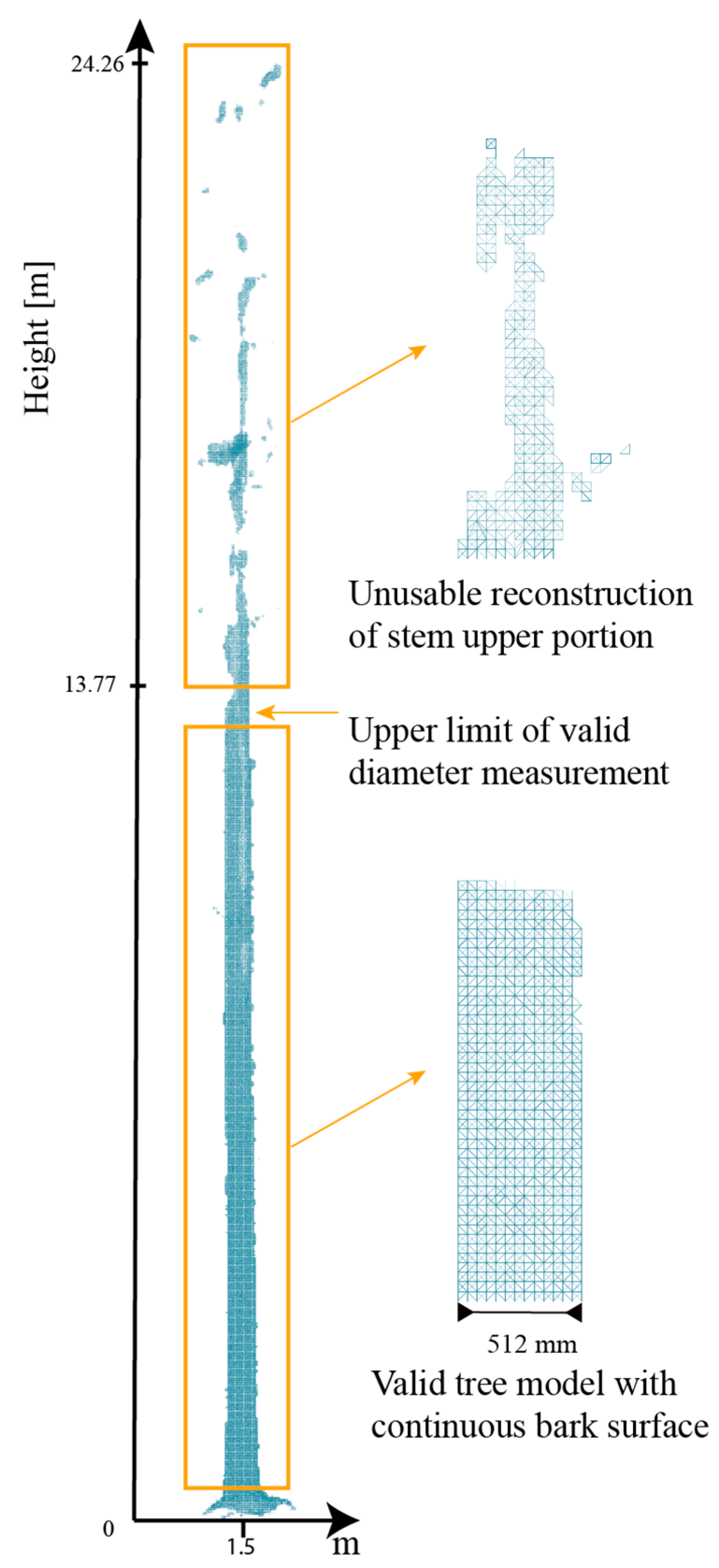
SfM successfully constructed the lower portion of the stem for all 18 trees (Figure 3). SfM was able to produce a usable reconstruction for only three trees above 13 m, and seven for 12 m. Therefore, diameters were measured only on the part of the stem where the tree surface was continuous and has a shape according to visual expectations.
The side-view measured diameters were constantly larger than the circumference-based diameters (Figure 4a), with a significant difference of 5.2 mm (p = 0.007 for the pair t-test). However, there were many heights for which the convex hull algorithm did not produce the expected polygon, as the PPC cross-section did not have the points evenly distributed along the circumference (Figure 4b). To obtain valid results, an algorithm that compensates for a lack of points in some area of the cross-section of the stem should be executed before the implementation of the convex hull algorithm. However, such algorithms are not readily available, and the augmentation of PPC introduces errors, as a model is used. Therefore, to carry the subsequent analyses with all of the ground measured diameters, the side-view measured diameters were used. The decision to use the side-view diameter instead of the circumferential diameter was enforced by an overestimation of diameter with more than 10 mm by both approaches, which requires a subsequent bias correction anyway.
Irrespective of the height of the stem, the PPC-measured mean diameter is constantly larger than the mean ground diameter (Figure 5), supporting the existence of bias. The variability of field and PPC measurements is similar along the stem, with a standard deviation between 61.9–82.7 mm and 40.0–88.4 mm, respectively (Figure 5). For heights <9 m, the variance decreased along the stem for both the ground and the PPC-based measurements, the largest occurring at 1.0 m for PPC (i.e., 782.9) and 1.3 m for field (i.e., 685.3). While diameter tapered with height, at 13 m we noticed the largest mean diameter (Figure 5) and the smallest variances for both the ground and PPC-based measurements. This unnatural situation occurred because only three measurements were recorded at 13 m, and those were for the largest trees (i.e., d1.3 >35 cm). Therefore, in further analyses, only the results for heights ≤12 m were considered.
The overall mean error is −17.2 mm, which is 6.3% larger than the mean diameter (Table 3). The estimates from the PPC are biased and not acceptable by the current field guides, which requires at least 5% accuracy. As expected, the MAB was larger than the bias but not significantly (i.e., 7.2% or 18.9 mm MAB). The RMSE was the largest fit statistic employed for assessment, and was almost 30% greater than the bias (i.e., 22.5 mm or 7.9%). The range of PPC–based measurements errors is fairly constant along the stem height (Figure 6). The smallest deviations of the PPC-based measurements occur close to the ground (i.e., ≤14 mm for heights ≤2.0 m). The largest deviation happens at 9 m, with the mean error equal to −23.7 mm, almost 10% of the corresponding diameter.
The Kolmogorov–Smirnov test supports the normal distribution of the difference between ground and PPC-based diameters (p > 0.1), except for the heights of 5 m and 6 m (p = 0.02 and 0.04, respectively). Grubbs’ test revealed no outliers in the data (p > 0.05), which justifies a t-test for assessing bias significance at all heights, except 5 m and 6 m. The t-test provided strong evidence (p < 0.01) that both bias and MAB are significantly different from 0, when applicable. For 5 m and 6 m, at which the t-test was not appropriate, the Wilcoxon test confirms the presence of significant bias.
To correct the bias, the preferred form of the Equation (5) has bi either 0 or 1. Coefficients different than 0 or 1 require field measurements, which in most instances are not only not available but preclude the remote sensing approach advocated by the paper. Multiple trials revealed that bias can be reduced with a linear function derived from Equation (4) (i.e., b1 and b4 are 1, the rest are 0):
where BC is the bias correction, is the PPC-based measurement error at d1.3 (i.e., d1.3 field–d1.3 PPC), and scaling error is the horizontal calibration error estimated by Agisoft.
Being unfitted to the data or the distribution of errors, Equation (7) will likely not eliminate the bias, but will reduce it. However, since the only field measurement needed is d1.3, which is commonly recorded anyway, Equation (7) delivered the intended results: measurement bias is operational and statistically insignificant. Nevertheless, a formal assessment of the residual error, errorht, residual, is required:
errorh, residual = error@h − BCh
The remaining bias was less than 1.8 mm (~0.5%), which was shown by the t-test to be not significantly different from 0 (p = 0.2). However, the t-test provides only empirical evidence that the bias was reduced to insignificant values. Nevertheless, assuming that bias is linearly related with height, the residual bias is approximately 10% of the d1.3 error, at most 1% of the diameter (proof in the Appendix A). For the 18 trees, the bias reduction was almost 10 times (i.e., 17.2/1.8 = 9.5 times), which proved that biased corrected PPC-measurements are accurate and precise.
3.2. Taper Equations
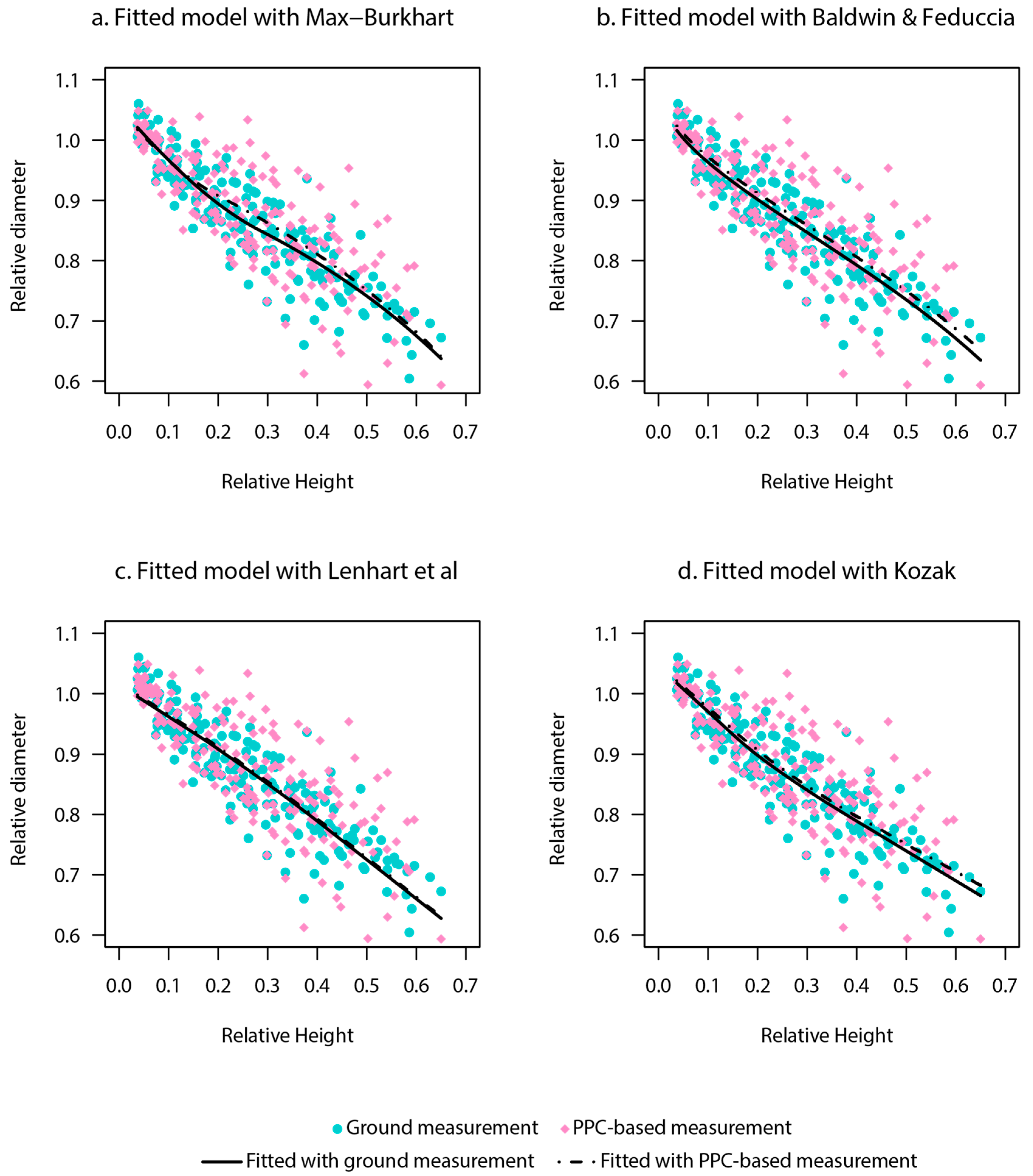
Since the highest valid stem measurement is at a stem height equal to 13 m, the four taper models evaluated the shape of the lower and middle portions of the stem. Only three of the four selected models (Table 2) could be used directly on the data, as they were developed specifically for loblolly pine. Irrespective of the source of data (i.e., field or PPC), all three models performed as intended by the authors with respect to the MAB, even though Lenhart et al. [3] had an MAB that was three times larger than the Max–Burhart or the Baldwin and Feduccia (Table 4). For the 18 trees, the bias was larger than in the original model (e.g., 5.7 mm vs. 3.6 mm for the Max–Burkhart), and significantly greater than other taper studies [69]. However, even though the RMSE was comparable with other taper studies [4,70], we refitted the models to the data, such that a formal assessment of the capacity to supply input data for taper modeling by PPC was executed.
When developed from field measurements, the models performed similarly, with all measures of fit being within the expected range: R2 > 0.97, bias < 1 mm, MAB and RMSE around 10 mm (Table 5). The models refitted from the PPC-based measurements supplied comparable fit statistics with the ground-based data (Table 6), except for bias, which was twice as large (i.e., 1.4 mm for Baldwin and Feduccia and 2.2 mm for Max–Burkhart vs. 0.6 mm and 0.9 mm, respectively). It should be noted that because the upper portion of the stem could not be rendered from the PPC, the upper inflection point of the Max–Burkhart equation was not identified. Therefore, a simplified version of the best Max–Burkhart equation (Table 2) was used for the PPC-based values (Equation (2) in the original article) Irrespective of the equation, the fit statistics are slightly higher for PPC-derived models than the ground-based models. Overall, the Kozak model performed the best, with the smallest bias, MAB, RMSE, and largest R2.
The Max–Burkhart model has the inflection point at a relative height of 0.29 for ground measurements and 0.20 for PPC measurements. However, the PPC-based model does not generate a significant estimate of α (p = 0.37), indicating that a single polynomial curve can approximate the tree bole. An apparent divergence between the field and PPC curves can be observed for the relative height between 0.18–0.40 (Figure 7a). The coefficients of the nonlinear term in the Baldwin and Feduccia model are the same (i.e., 0.24), while the ones for the linear term are practically indistinguishable between the two datasets (Figure 7b). The model fit from the ground measurements is superior to the PPC-based model (i.e., the MAB is 9.2 mm vs. 13.3 mm, and the RMSE is 13.2 mm vs. 18.3 mm, respectively). Similarly to the Baldwin and Feduccia model, regardless of the measurement’s source, the Lenhart et al. model has the same estimates of the power term (Figure 7c). Mirroring the Max–Burkhart model, Kozak’s model has insignificant estimates for two coefficient (i.e., p >0.10 for b2 and b3). The lack of significance is noticed for relative heights >0.5 (Figure 7d).
The cross-validation of the PPC-based models with the field data reveals agreement for all fit statistics (Table 7), with R2 ≥ 0.97 irrespective of the model type, bias < 4 mm, MAB < 10 mm, and RMSE < 15 mm. Even though Kozak’s model proved to be most suited to represent diameter variation along the stem, the Baldwin and Feduccia model, which is simpler, supplied similar fit statistics with a significant increase in parsimony.
4. Discussion
Current applications of SfM in forest inventory are limited by irregular stem geometry and a complex background, which present challenges for camera location, key point extraction, and geo-reference under dense canopy. An oblique perspective limits the ability for 3D reconstruction of the entire tree, particularly the higher portion of the trunk. Therefore, the diameter measurements were below 12 m (i.e., the first two logs), which is approximately half of the total tree height. Nevertheless, higher diameters can be measured if the photographic information is captured with unmanned aerial vehicles flying along and around the tree.
Lighting and the background of the object to be rendered with SfM plays a significant role in the accuracy of the reproduction process [71,72], particularly the lack of features and low light (called “bad lighting” by Koutsoudis et al. [71]). Considering that all images were acquired under canopy where limited light is present, we have chosen only spring and summer bright days, with almost no cloud coverage and no rain for three days. The lack of details and a homogeneous background were not a concern, as forest provides plenty of variation to allow for the identification of a multitude of key points.
The diameter measurements directly from PPCs are constantly higher than ground measurements, which is the result of two assumptions: first, the stem is circular, and second, the length along the stem is measured without error. This combination impacted on the AutoCAD measurements, as the rotation of the stem could, and likely would, lead to small variations in diameter at the same location along the stem. Therefore, besides calibration errors, measurement errors are also present. The bias correction equation that we proposed (Equation (7)) is practical and intuitive rather than mathematically-based. The measurement bias seems to be positively related to the stem height. We assumed that the projective direction of the camera is almost horizontal, at the eye of the operator; therefore, the best-estimated diameter is d1.3. The measurement error expands along the stem as the distance becomes increasingly further from the projection’s center. Consequently, we select the relative height as the correcting term. A higher order polynomial of relative height, or even a rotation correction term, could lead to better results than the proposed affine transformation (Equation (7)), as the images are restructured with a nonlinear process. It is possible that accuracy is influenced by errors occurring from multiple directions [73]. Even so, the largest error, relative to diameter, was 4% (i.e., at 12 m), the rest being ≤2%. The accuracy and precision of diameter measurements from PPC are not the only advantages of using 3D reconstruction from images. The PPC allows for diameter measurements at any height, not only at preset ones (e.g., every meter). Furthermore, high-density PPC supplies information for the detection and estimation of trunk defects, such as catface or sweep.
The results show that the equations developed from the PPC-based measurements are comparable with the equations developed from the ground-based measurements, when the same model forms were applied. The four models developed by the PPC-based measurements could be used to estimate the ground diameter with an accuracy of <4 mm. The bias of the PPC-based diameter models does not vary remarkably among the four model forms. The most evident difference between the ground and PPC-based models occurs for the Max–Burkhart model (Figure 7a). The Kozak model 02 was not originally developed for the diameter estimation of loblolly pine. However, the goodness-of-fit of the Kozak models is slightly better than other models, consistent with the finding of Li and Weiskittel [74]. According to their study, Kozak model 02 will fit the diameters of other species across a wide range of biogeographic zones [74]. Diameters estimated with the Baldwin and Feduccia [2] equation are the closest to the ground measurements at a relative height of >0.22, compared with the Max–Burkhart and Lenhart et al. equations. A possible explanation of the relatively weak performance of the Lenhart et al. (1987) equation could rest with its development, which was confined to small trees (d1.3 < 33 cm). Nevertheless, our study results show that the selection of model form would not significantly influence the model fit. Among the four models selected for taper assessment, we consider the Baldwin and Feduccia [2] approach to be the most trustworthy, as it is intuitive and relatively simple. The Kozak [4] model 02 outperformed all other models, but its lack of realism and low parsimony (e.g., six parameters compared to two for Baldwin and Feduccia) is not appealing. In fact, the difference between Kozak’s model 02 and the Baldwin and Feduccia model is minute, as bias, MAB, and RMSE are almost the same (Table 7). Therefore, the PPC measurements can be used not only for the direct estimation of diameter (bias was <2 mm), but also for taper modeling (bias < 4 mm and R2 ≥ 0.97).
Diameter estimation and taper modeling were possible for loblolly pine because the crown is concentrated on a small portion along the trunk (usually < 30%) and a lack of dead branches on the lower portion of the stem. However, for species that keep for long time their lower branches, such as Douglas fir (Pseudotsuga menziesii Mirb.) or Norway spruce (Picea abies L.), the usage of SfM is difficult not only because of the difficulty to navigate but also because of the poor light conditions. In these situations, a combination of active–passive sensors could deliver the desired point clouds.
The PPC proved that it can be used for modeling taper, and consequently the amount and type of products that can be obtained from individual stems. We expect that subsequent studies on taper, particularly for genetic studies where branching is also important, will be almost entirely based on PPC. New equipment that allows diameter measurements along the stem, such as Criterion RD by Laser Technology, did not reduce significantly the time to acquire accurate data significantly. Furthermore, while measurements based optical devices exhibit an increase in variability with distance from the tree, the PPC is not affected by these issues. Large sample size balances the estimates of various taper modeling methods, but all approaches, except the ones based on PPC, are either expensive (i.e., terrestrial lidar) or have larger variability. The costs of producing PPC will decrease, which would make it even more attractive. We expect that real time PPC creation will occur in the next decade, which will allow for the estimation of products during forest operations, which will increase the value of each stand.
5. Conclusions
In this paper, we proposed an accurate procedure for measuring diameter along the stem from consumer grade cameras. Limited training and fieldwork is required for capturing oblique images of the trees and for the execution of the scaling operation. The images are rendered to a 3D point cloud using a structure form motion algorithm, hence the name photogrammetric point cloud (PPC). Diameter measurements executed on the PPC along the stem are biased, overestimating the real diameter. However, a simple, intuitive, and easy to implement correction will reduce the bias to millimeters, at most ≤2%. Diameter measurements from PPC can successfully replace ground measurements not only by being accurate while reducing the costs and time, but also by allowing a continuous examination of the stem. Therefore, taper models can be developed from PPC-based measurements that would trace closely the stem, (e.g., every 10 cm). We assessed the diameter measurements with four popular taper models, and we found no operational and statistical difference between the models developed from ground data and from PPC-corrected data. In fact, two models (Kozak [4] model 02 and Baldwin and Feduccia [2]) had a bias of less than 1 mm. Although the application of SfM is still limited in the context of vegetation with high complexity, our results suggest that PPC-based models are as accurate as conventional inventory. A reconstruction of the entire stem can be achieved by combining images acquired by unmanned aerial systems with ground-based photographs. The examination of the entire trunk can expand beyond dendrometric attributes, such as diameter or length, and can include stem defects, such as catface, knots, or sweep. For accurate product estimation in the lower portion of the bole (e.g., the first two logs), our results recommend the replacement of taper with PPC, as it is fast, and more accurate and precise.
Author Contributions
Rong Fang executed the PPC reconstruction, assessed the bias of the measurements, and developed taper models. Bogdan Strimbu designed the methodology, coordinated data acquisition, and estimated the residual bias. Both authors contributed to the writing of the paper.
Conflicts of Interest
The authors declare no conflict of interest.
Appendix A. Estimation of Residual Bias after Application of Equation (7)
The selected function to eliminate bias Equation (7) was not tailored to the data or to the error structure. Therefore, it is likely that bias was reduced not eliminated. After bias reduction, the error, εh, becomes:
where the h subscript represents the height at which the respective statistic is computed.
εh = errorh − BCh = dh,field − dh,PPC − d1.3,field − d1.3,PPC − RH × errorAgisoft
According to Agisoft documentation, the scaling error is a result of the difference between the distance estimated from the point cloud and the distance assigned by the operator after identification of two points inside PPC:
errorAgisoft = dPPC − doperator
Figure 5 suggests that a linear function could describe the relationship between bias and relative height (RH). A simple linear regression between error and relative height supplied a significant equation (p = 0.02), with both coefficients significant:
errorh = −1.36 − 1.42 × RH
The two coefficients were close to the d1.3 error, 1.20 mm, (i.e., intercept in Equation (7)) and to reported error by Agisoft, 1.22, (i.e., slope in Equation (7)). In fact, there was no significant difference between the coefficients of regression A3 and the two statistics. The choice of which one will be intercept and which one slope was driven by the magnitude of the bias reduction as well as the variation. The model with d1.3 error as slope has a residual bias of 0.15 mm, while the alternative was 0.18 mm. However, even though the bias was smaller when d1.3 error was slope, the variance was larger (i.e., 2.97 vs. 2.88), which suggested selection of the Equation (7) to reduce the bias.
To assess bias we computed the expectation of the residual errors εh:
The diameter estimated by the operator from Agisoft suffers from the same lack of accuracy as the one measured in the field; therefore, it can be assumed that
Table 3 reveals that errord1.3 is the smallest among all heights (except for height 9 m, which likely is a random occurrence), a direct result of closeness to the operator, and consequently to the camera, of that section of the tree. Figure 6 supports the existence of a linear relationship between expectation of the error anywhere on the stem and d1.3 error:
where b is a coefficient.
Based on Equations (A5) and (A6), Equation (A4) can be rearranged as:
Equation (A7) depends on coefficient b, whose value can be approximated from the observation that
Therefore, the remaining bias after the application of Equation (7) is 1.3 × E[error d1.3]/(total height). Considering that field measurements are executed for stands that require immediate attention, such as thinning or regeneration harvests, it can be assumed that the total height of the trees is larger than 13 m, which mean that the expected residual bias is less than 10% of E[error d1.3]. According to Table 3, E[error d1.3] is the smallest among errors at all heights (except for 12 m), therefore the residual bias is expected to be approximately 1 mm.
References
- Max, T.A.; Burkhart, H.E. Segmented polynomial regression applied to taper equations. For. Sci. 1976, 22, 283–289. [Google Scholar]
- Baldwin, V.C.; Feduccia, D.P. Compatible tree-volume and upper-stem diameter equations for plantation loblolly pines in the west gulf region. South. J. Appl. For. 1991, 15, 92–97. [Google Scholar]
- Lenhart, J.D.; Hackett, T.L.; Laman, C.J.; Wiswell, T.J.; Blackard, J.A. Tree content and taper functions for loblolly and slash pine trees planted on non-old-fields in east texas. South. J. Appl. For. 1987, 11, 147–151. [Google Scholar]
- Kozak, A. My last words on taper equations. For. Chron. 2004, 80, 507–515. [Google Scholar] [CrossRef]
- Avery, T.E.; Burkhart, H. Forest Measurements; Mcgraw-Hill Ryerson: New York, NY, USA, 2001; p. 480. [Google Scholar]
- Husch, B.; Beers, T.W.; Kershaw, J.A. Forest Mensuration, 4th ed.; Wiley: New Yourk, NY, USA, 2002; p. 456. [Google Scholar]
- Burkhart, H.E.; Tome, M. Modeling Forest Trees and Stands; Springer: New York, NY, USA, 2012; p. 460. [Google Scholar]
- Lee, J.-H.; Ko, Y.; McPherson, E.G. The feasibility of remotely sensed data to estimate urban tree dimensions and biomass. Urban For. Urban Green. 2016, 16, 208–220. [Google Scholar] [CrossRef]
- Lu, D.; Chen, Q.; Wang, G.; Liu, L.; Li, G.; Moran, E. A survey of remote sensing-based aboveground biomass estimation methods in forest ecosystems. Int. J. Dig. Earth 2016, 9, 63–105. [Google Scholar] [CrossRef]
- Williams, M.S.; Cormier, K.L.; Briggs, R.G.; Martinez, D.L. Evaluation of the barr & stroud fp15 and criterion 400 laser dendrometers for measuring upper stem diameters and heights. For. Sci. 1999, 45, 53–61. [Google Scholar]
- Shimizu, A.; Yamada, S.; Arita, Y. Diameter measurements of the upper parts of trees using an ultra-telephoto digital photography system. Open J. For. 2014, 4, 316–326. [Google Scholar] [CrossRef]
- Nunes, M.H.; Görgens, E.B. Artificial intelligence procedures for tree taper estimation within a complex vegetation mosaic in brazil. PLoS ONE 2016, 11, e0154738. [Google Scholar] [CrossRef] [PubMed]
- Cushman, K.C.; Muller-Landau, H.C.; Condit, R.S.; Hubbell, S.P. Improving estimates of biomass change in buttressed trees using tree taper models. Methods Ecol. Evol. 2014, 5, 573–582. [Google Scholar] [CrossRef]
- Saarinen, N.; Kankare, V.; Vastaranta, M.; Luoma, V.; Pyörälä, J.; Tanhuanpää, T.; Liang, X.; Kaartinen, H.; Kukko, A.; Jaakkola, A.; et al. Feasibility of terrestrial laser scanning for collecting stem volume information from single trees. ISPRS J. Photogramm. Remote Sens. 2017, 123, 140–158. [Google Scholar] [CrossRef]
- Olofsson, K.; Holmgren, J. Single tree stem profile detection using terrestrial laser scanner data, flatness saliency features and curvature properties. Forests 2016, 7, 207. [Google Scholar] [CrossRef]
- You, L.; Tang, S.; Song, X.; Lei, Y.; Zang, H.; Lou, M.; Zhuang, C. Precise measurement of stem diameter by simulating the path of diameter tape from terrestrial laser scanning data. Remote Sens. 2016, 8, 717. [Google Scholar] [CrossRef]
- Henning, J.G.; Radtke, P.J. Detailed stem measurements of standing trees from ground-based scanning lidar. For.Sci. 2006, 52, 67–80. [Google Scholar]
- Coble, D.W.; Hilpp, K. Compatible cubic-foot stem volume and upper-stem diameter equations for semi-intensive plantation grown loblolly pipe trees in east Texas. South. J. Appl. For. 2006, 30, 132–141. [Google Scholar]
- Farrar, R.M. Stem-profile functions for predicting multiple-product volumes in natural longleaf pines. South. J. Appl. For. 1987, 11, 161–167. [Google Scholar]
- Westfall, J.A. Modifying Taper-Derived Merchantable Height Estimates to Account for Tree Characteristics; USDA Forest Service: Washington, DC, USA, 2006; p. 126. [Google Scholar]
- Newnham, R.M. Variable-form taper functions for four Alberta tree species. Can. J. For. Res. 1992, 22, 210–223. [Google Scholar] [CrossRef]
- Lowe, D.G. Distinctive image features from scale-invariant keypoints. Int. J. Comput. Vis. 2004, 60, 91–110. [Google Scholar] [CrossRef]
- Smith, R.C.; Cheeseman, P. On the representation and estimation of spatial uncertainty. Int. J. Robot. Res. 1986, 5, 56–68. [Google Scholar] [CrossRef]
- Harris Geospatial Solutions. Envi; Exelis Visual Information Solutions: Boulder, CO, USA, 2016. [Google Scholar]
- Hexagon Geospatial. Erdas Imagine; Hexagon AB: Stockholm, Switzerland, 2016. [Google Scholar]
- Schindler, K.; Bischof, H. On robust regression in photogrammetric point clouds. In Proceedings of the Pattern Recognition: 25th Dagm Symposium, Magdeburg, Germany, 10–12 September 2003; Michaelis, B., Krell, G., Eds.; Springer: Berlin/Heidelberg, Germany, 2003; pp. 172–178. [Google Scholar]
- Soule, S.; Maurice, K.; Walcher, W.; Szabo, J. Advanced Point Cloud Generation for Photogrammetric Modeling of Complex 3d Objects. In Proceedings of the International Conference on Image Processing, Rochester, NY, USA, 24–28 June 2002; IEEE: New York, NY, USA, 2002; Volume 523, pp. 529–532. [Google Scholar]
- Lucas, B.D.; Kanade, T. An Iterative Image Registration Technique with an Application to Stereo Vision. In Proceedings of the International Joint Conference on Artificial Intelligence (IJCAI), Vancouverm, BC, Canada, 24–28 August 1981; pp. 674–679. [Google Scholar]
- Haralick, R.M. Digital step edges from zero crossing of second directional derivatives. IEEE Trans. Patt. Anal. Mach. Intell. 1984, 1, 58–68. [Google Scholar] [CrossRef]
- Agisoft LLC. Agisoft Photoscan; Agisoft: St. Petersburg, Russia, 2014. [Google Scholar]
- Pix4d; Pix4D: Lausanne, Switzerland, 2014.
- Wu, C. Visualsfm v0.5.26. Available online: http://ccwu.me/vsfm/ (accessed on 11 July 2017).
- Fritz, A.; Kattenborn, T.; Koch, B. Uav-based photogrammetric point clouds—Tree stem mapping in open stands in comparison to terrestrial laser scanner point clouds. Int. Arch. Photogramm. Remote Sens. Spat. Inf. Sci. 2013, 40, 141–146. [Google Scholar] [CrossRef]
- Forsman, M.; Börlin, N.; Holmgren, J. Estimation of tree stem attributes using terrestrial photogrammetry with a camera rig. Forests 2016, 7, 61. [Google Scholar] [CrossRef]
- Mikita, T.; Janata, P.; Surový, P. Forest stand inventory based on combined aerial and terrestrial close-range photogrammetry. Forests 2016, 7, 165. [Google Scholar] [CrossRef]
- Mensah, S.; Glèlè Kakaï, R.; Seifert, T. Patterns of biomass allocation between foliage and woody structure: The effects of tree size and specific functional traits. Ann. For. Res. 2016, 1, 59. [Google Scholar] [CrossRef]
- Garber, S.M.; Maguire, D.A. Modeling stem taper of three central oregon species using nonlinear mixed effects models and autoregressive error structures. For. Ecol. Manag. 2003, 179, 507–522. [Google Scholar] [CrossRef]
- Valentine, H.T.; Gregoire, T.G. A switching model of bole taper. Can. J. For. Res. 2001, 31, 1400–1409. [Google Scholar] [CrossRef]
- Nyland, R.D. Silviculture. Concepts and Applications; McGraw-Hill: New York, NY, USA, 1996; p. 633. [Google Scholar]
- Smith, D.M. The Practice of Silviculture: Applied Forest Ecology, 9th ed.; Wiley: New York, NY, USA, 1997; p. 537. [Google Scholar]
- Turner, D.; Lucieer, A.; Wallace, L. Direct georeferencing of ultrahigh-resolution uav imagery. IEEE Trans. Geosci. Remote Sens. 2014, 52, 2738–2745. [Google Scholar] [CrossRef]
- Liang, X.L.; Jaakkola, A.; Wang, Y.S.; Hyyppa, J.; Honkavaara, E.; Liu, J.B.; Kaartinen, H. The use of a hand-held camera for individual tree 3d mapping in forest sample plots. Remote Sens. 2014, 6, 6587–6603. [Google Scholar] [CrossRef]
- Robertson, F.D. Timber Cruising Handbook; USDA Forest Service: Washington, DC, USA, 2000; p. 268. [Google Scholar]
- Autodesk. Autocad Civil 3d; Autodesk: SanRafael, CA, USA, 2016. [Google Scholar]
- Barber, C.B.; Dobkin, D.P.; Huhdanpaa, H. The quickhull algorithm for convex hulls. ACM Trans. Math. Softw. 1996, 22, 469–483. [Google Scholar] [CrossRef]
- Maas, H.G.; Bienert, A.; Scheller, S.; Keane, E. Automatic forest inventory parameter determination from terrestrial laser scanner data. Int. J. Remote Sens. 2008, 29, 1579–1593. [Google Scholar] [CrossRef]
- The Math Works Inc. Matlab R2017a; The Math Works Inc.: Natick, MA, USA, 2017. [Google Scholar]
- Daniilidis, K.; Spetsakis, M.E. Understanding noise sensitivity in structure from motion. In Visual Navigation; Aloimonos, Y., Ed.; Lawrence Erlbaum Associates: Hillsdale, NJ, USA, 1996; pp. 61–88. [Google Scholar]
- Stängle, S.M.; Sauter, U.H.; Dormann, C.F. Comparison of models for estimating bark thickness of picea abies in southwest germany: The role of tree, stand, and environmental factors. Ann. For. Sci. 2017, 74, 16. [Google Scholar] [CrossRef]
- Montealegre, A.; Lamelas, M.; Riva, J. Interpolation routines assessment in als-derived digital elevation models for forestry applications. Remote Sens. 2015, 7, 8631–8654. [Google Scholar] [CrossRef]
- Powell, S.L.; Cohen, W.B.; Healey, S.P.; Kennedy, R.E.; Moisen, G.G.; Pierce, K.B.; Ohmann, J.L. Quantification of live aboveground forest biomass dynamics with landsat time-series and field inventory data: A comparison of empirical modeling approaches. Remote Sens. Environ. 2010, 114, 1053–1068. [Google Scholar] [CrossRef]
- Bilskie, M.V.; Hagen, S.C. Topographic accuracy assessment of bare earth lidar-derived unstructured meshes. Adv. Water Resour. 2013, 52, 165–177. [Google Scholar] [CrossRef]
- Schabenberger, O.; Pierce, F.J. Contemporary Statistical Models for the Plant and Soil Sciences; CRC Press: Boca Raton, FL, USA, 2002; p. 730. [Google Scholar]
- Neter, J.; Kutner, M.H.; Nachtsheim, C.J.; Wasserman, W. Applied Linear Statistical Models; WCB McGraw-Hill: Boston, MA, USA, 1996; p. 1408. [Google Scholar]
- Grubbs, F.E. Sample criteria for testing outlying observations. Ann. Math. Stat. 1950, 21, 27–58. [Google Scholar] [CrossRef]
- Thode, H.C. Testing for Normality; Marcel Dekker: New York, NY, USA, 2002; p. 368. [Google Scholar]
- Hollander, M.; Wolfe, D.A. Nonparametric Statistical Methods; John Wiley and Sons: New York, NY, USA, 1973; p. 503. [Google Scholar]
- SAS Institute. Sas 9.1; SAS Institute: Cary, NC, USA, 2010. [Google Scholar]
- Cao, Q.V. Calibrating a segmented taper equation with two diameter measurements. South. J. Appl. For. 2009, 33, 58–61. [Google Scholar]
- Trincado, G.; Burkhart, H.E. A generalized approach for modeling and localizing stem profile curves. For. Sci. 2006, 52, 670–682. [Google Scholar]
- Williams, M.S.; Reich, R.M. Exploring the error structure of taper equations. For. Sci. 1997, 43, 378–386. [Google Scholar]
- Grothendieck, G. Nls2: Non-Linear Regression with Brute Force, Version 0.2. The Comprehensive R Archive Network (CRAN), 2013. Available online: https://cran.r-project.org/web/packages/nls2/nls2.pdf (accessed on 11 July 2017).
- R Core Team. R: A Language and Environment for Statistical Computing; R Foundation for Statistical Computing: Vienna, Austria, 2016. [Google Scholar]
- Jiang, L.-C.; Liu, R.-L. Segmented taper equations with crown ratio and stand density for dahurian larch (larix gmelinii) in Northeastern China. J. For. Res. 2011, 22, 347–352. [Google Scholar] [CrossRef]
- Sharma, M.; Zhang, S.Y. Variable-exponent taper equations for jack pine, black spruce, and balsam fir in eastern canada. For. Ecol. Manag. 2004, 198, 39–53. [Google Scholar] [CrossRef]
- Grimmett, G.D.; Stirzaker, D.R. Probability and Random Processes; Oxford University Press: New York, NY, USA, 2002; p. 600. [Google Scholar]
- Poole, D. Linear Algebra; Thomson Brooks/Cole: Toronto, ON, Canada, 2005; p. 712. [Google Scholar]
- Vidal, C.; Alberdi, I.A.; Mateo, L.H.; Redmond, J.J. National Forest Inventories: Assessment of Wood Availability and Use; Springer: Cham, Switzerland, 2016; p. 845. [Google Scholar]
- Lejeune, G.; Ung, C.-H.; Fortin, M.; Guo, X.; Lambert, M.-C.; Ruel, J.-C. A simple stem taper model with mixed effects for boreal black spruce. Eur. J. For. Res. 2009, 128, 505–513. [Google Scholar] [CrossRef]
- Newberry, J.D.; Burkhart, H.E. Variable-form stem profile models for loblolly pine. Can. J. For. Res. 1986, 16, 109–114. [Google Scholar] [CrossRef]
- Koutsoudis, A.; Vidmar, B.; Ioannakis, G.; Arnaoutoglou, F.; Pavlidis, G.; Chamzas, C. Multi-image 3d reconstruction data evaluation. J. Cult. Herit. 2014, 15, 73–79. [Google Scholar] [CrossRef]
- Nikolov, I.; Madsen, C. Benchmarking close-range structure from motion 3d reconstruction software under varying capturing conditions. In Digital Heritage. Progress in Cultural Heritage: Documentation, Preservation, Proceedings of the Protection: 6th International Conference, Euromed 2016, Nicosia, Cyprus, 31 October–5 November 2016, Part I; Ioannides, M., Fink, E., Moropoulou, A., Hagedorn-Saupe, M., Fresa, A., Liestøl, G., Rajcic, V., Grussenmeyer, P., Eds.; Springer International Publishing: Cham, Switzerland, 2016; pp. 15–26. [Google Scholar]
- Weng, J.; Huang, T.S.; Ahuja, N. Motion and structure from two perspective views: Algorithms, error analysis, and error estimation. IEEE Trans. Patt. Anal. Mach. Intell. 1989, 11, 451–476. [Google Scholar] [CrossRef]
- Li, R.; Weiskittel, A.R. Comparison of model forms for estimating stem taper and volume in the primary conifer species of the north american acadian region. Ann. For. Sci. 2010, 67, 302. [Google Scholar] [CrossRef]
Figure 1.
Area showing the location of the trees: (a) general position of the trees within Louisiana; (b) locations of all the trees photographed and cut; (c) the four most southern trees. The yellow arrows show the size of a rectangular box (highlighted) containing the southern four trees; (d) lidar point cloud of the rectangle containing the southern four trees from (c). The arrows from (c) to (d) indicate the top of each tree in the point cloud.
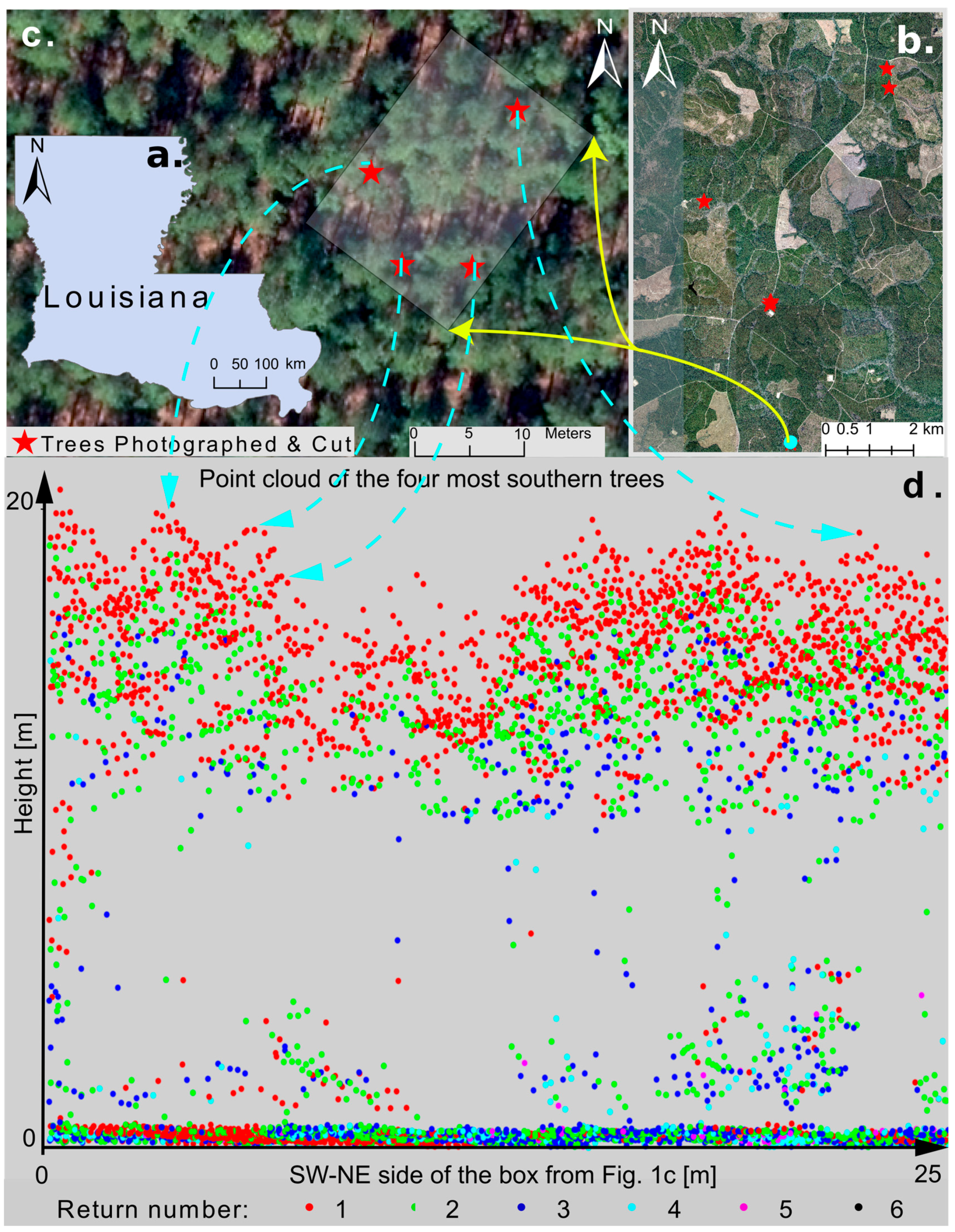
Figure 2.
Workflow of the photogrammetric-based stem reconstruction and diameter measurement. (a) Field photographs for an individual tree; (b) structure from motion (SfM) process of reconstruction (tie points, densified points, surface); (c) scaling the photogrammetric point clouds (PPC) with reference bar and d1.3; (d) diameter measurements in AutoCAD.

Figure 3.
An example of a reconstructed stem, with the lower part continuous, (i.e., measurable surface), and the upper part fragmented (i.e., unsuitable for accurate measurements).
Figure 3.
An example of a reconstructed stem, with the lower part continuous, (i.e., measurable surface), and the upper part fragmented (i.e., unsuitable for accurate measurements).

Figure 4.
Diameter measurements on cross sections of the stem (a) successfully identified by the convex hull algorithm at height 4 m, (b) unsuccessful identified by the convex hull algorithm at height 11 m. The red line is the circumference of the tree as computed by the convex hull algorithm.
Figure 4.
Diameter measurements on cross sections of the stem (a) successfully identified by the convex hull algorithm at height 4 m, (b) unsuccessful identified by the convex hull algorithm at height 11 m. The red line is the circumference of the tree as computed by the convex hull algorithm.
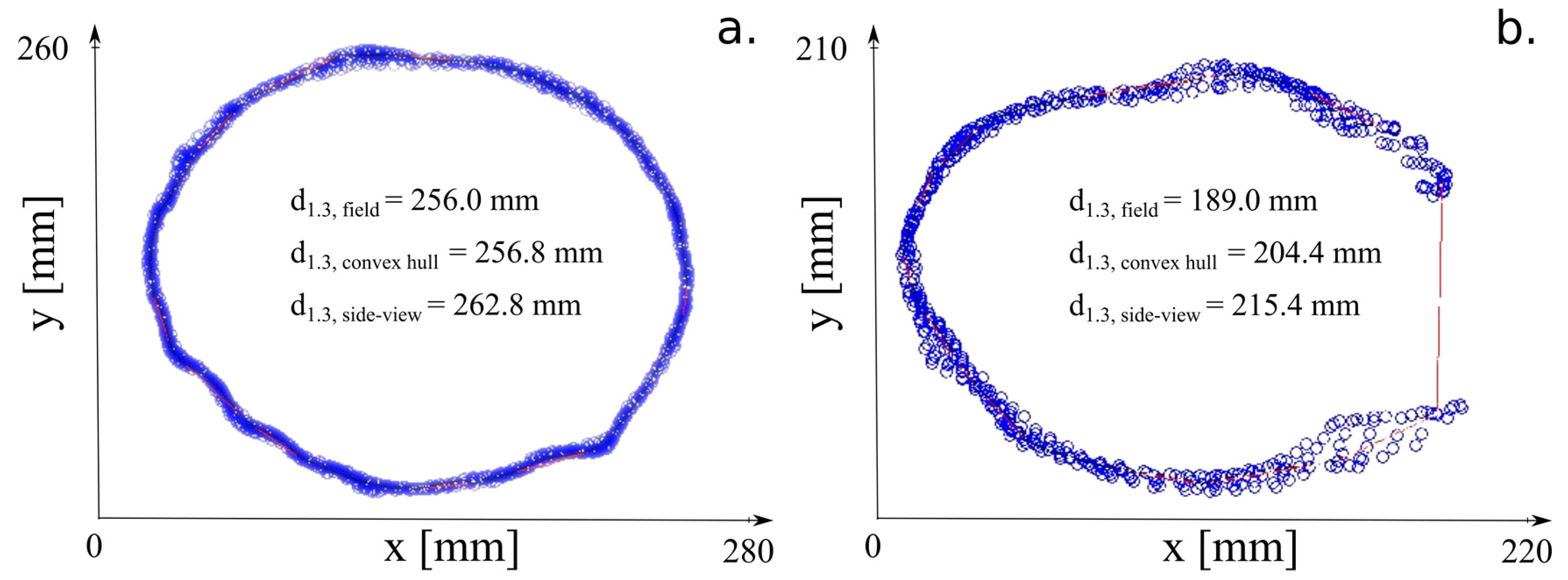
Figure 5.
Variation with height of diameters measured in the field and from the PPC for the side-view measurements.
Figure 5.
Variation with height of diameters measured in the field and from the PPC for the side-view measurements.
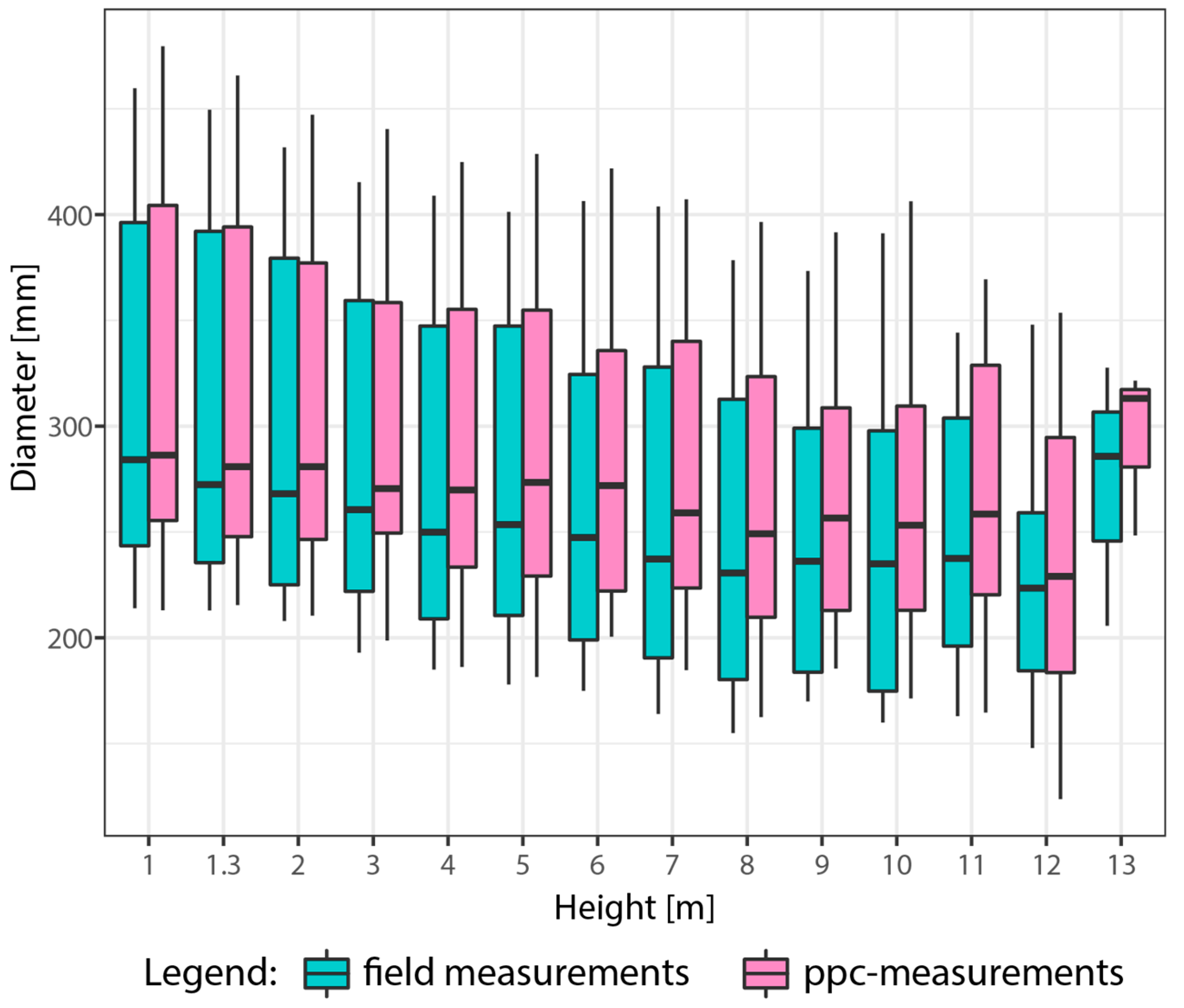
Figure 6.
The PPC-based error vs. the stem height; (a) uncorrected (b) after bias correction with Equation (7). The dots represents outliers, which are estimated using the interquartile range approach.
Figure 6.
The PPC-based error vs. the stem height; (a) uncorrected (b) after bias correction with Equation (7). The dots represents outliers, which are estimated using the interquartile range approach.
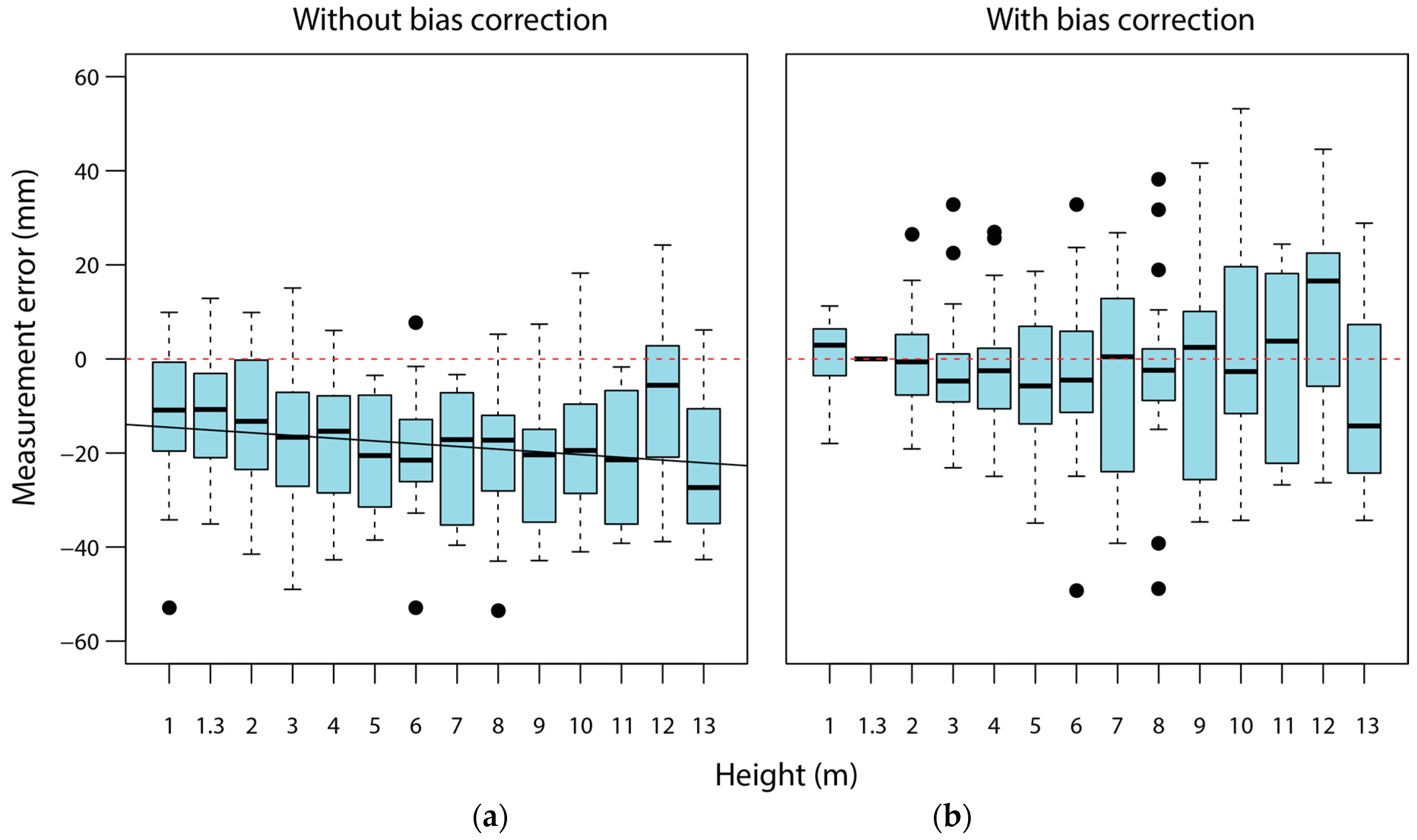
Figure 7.
Comparisons of the models developed with the PPC-based measurement and the ground-based measurement. (a) Max and Burkhart (b) Baldwin and Feduccia (c) Lenhart et al. (d) Kozak.
Figure 7.
Comparisons of the models developed with the PPC-based measurement and the ground-based measurement. (a) Max and Burkhart (b) Baldwin and Feduccia (c) Lenhart et al. (d) Kozak.


Table 1.
Parameter for generation of the PPC with SfM implemented in Agisoft.
| Photo Alignment | Point Cloud Densification | Mesh Building | |||
|---|---|---|---|---|---|
| Accuracy | Medium & High | Quality | High | Face count | High |
| Key points | 100,000 | Depth filtering | Disabled | Interpolation | Disabled |
| Tie points | 60,000 | ||||
Table 2.
Taper equations used for modeling diameter outside bark.
| Model | Equation |
|---|---|
| Max–Burkhart Equation (4) in original paper | |
| Baldwin-Feduccia Equation (2) in original paper | |
| Lenhart et al. Equation (26) in original paper | |
| Kozak Equation (3) in original paper |
Table 3.
Variation along the stem of diameter measurement error from PPC. Diameter is the diameter measured in the field. RMSE, root mean square error.
Table 3.
Variation along the stem of diameter measurement error from PPC. Diameter is the diameter measured in the field. RMSE, root mean square error.
| Height | Diameter | Bias | Mean Absolute Error | RMSE | |||
|---|---|---|---|---|---|---|---|
| [m] | [mm] | [mm] | [%] | [mm] | [%] | [mm] | [%] |
| 1 | 312 | −12.1 | −3.9 | 14.8 | 4.8 | 19.4 | 6.2 |
| 1.3 | 306 | −12.0 | −3.9 | 13.5 | 4.4 | 17.1 | 5.6 |
| 2 | 296 | −13.5 | −4.6 | 16.1 | 5.4 | 20.4 | 6.9 |
| 3 | 287 | −16.4 | −5.7 | 19.2 | 6.7 | 22.5 | 7.8 |
| 4 | 278 | −17.2 | −6.2 | 18.2 | 6.6 | 22.4 | 8.0 |
| 5 | 270 | −20.3 | −7.5 | 20.3 | 6.5 | 23.3 | 8.6 |
| 6 | 263 | −19.5 | −7.4 | 20.3 | 7.7 | 23.3 | 8.9 |
| 7 | 256 | −20.0 | −7.8 | 20.0 | 7.8 | 23.8 | 9.3 |
| 8 | 247 | −20.0 | −8.1 | 20.5 | 8.3 | 24.2 | 9.8 |
| 9 | 244 | −22.4 | −9.2 | 23.8 | 9.8 | 26.7 | 11.0 |
| 10 | 242 | −18.2 | −7.5 | 20.9 | 8.6 | 22.9 | 9.4 |
| 11 | 249 | −19.9 | −8.0 | 19.9 | 8.0 | 24.1 | 9.7 |
| 12 | 229 | −8.1 | −3.5 | 18.1 | 7.9 | 22.1 | 9.6 |
| Total | - | −17.2 | −6.3 | 18.8 | 6.9 | 22.5 | 8.2 |
Table 4.
Performance of existing taper models on field and PPC-based measurements. Max–Burkhart Model 4 was used for assessment. MAB, mean absolute bias.
Table 4.
Performance of existing taper models on field and PPC-based measurements. Max–Burkhart Model 4 was used for assessment. MAB, mean absolute bias.
| Equation | Coeff | Original | Bias [mm] | MAB [mm] | RMSE [mm] | |||
|---|---|---|---|---|---|---|---|---|
| Field | PPC | Field | PPC | Field | PPC | |||
| Max–Burkhart | b1 | −3.0257 | 5.7 | 12.4 | 14.1 | 19.4 | 18.1 | 24.4 |
| b2 | 1.4586 | |||||||
| b3 | −1.4464 | |||||||
| b4 | 39.1081 | |||||||
| a1 | 0.7431 | |||||||
| a2 | 0.1125 | |||||||
| Baldwin–Feduccia | b1 | 1.22467 | −6.2 | 0.1 | 14.7 | 17.9 | 18.6 | 21.9 |
| b2 | 0.3563 | |||||||
| Lenhart et al. | b | 0.841837 | 16.0 | 23.2 | 19.5 | 25.4 | 27.3 | 34.9 |
Table 5.
Taper models developed from ground-based measurements.
| Equation | Coeff. | Data | p-Value | R2 | Bias [mm] | MAB [mm] | RMSE [mm] | RMSE [%] |
|---|---|---|---|---|---|---|---|---|
| Max–Burkhart | b1 | −0.48 | <0.001 | 0.98 | −0.9 | 8.7 | 12.2 | 4 |
| b2 | −0.41 | 0.01 | ||||||
| b3 | 2.72 | 0.02 | ||||||
| a | 0.29 | <0.001 | ||||||
| Baldwin–Feduccia | b1 | 1.11 | <0.001 | 0.98 | −0.6 | 8.6 | 11.7 | 5 |
| b2 | 0.24 | <0.001 | ||||||
| Lenhart et al. | b | 0.5288 | 0.01 | 0.97 | −2.0 | 9.8 | 12.9 | 5 |
| Kozak | a0 | 1.35 | <0.001 | 0.98 | −0.01 | 8.4 | 11.9 | 5 |
| a1 | 0.94 | <0.001 | ||||||
| b0 | 0.19 | <0.001 | ||||||
| b1 | 0.3 | 0.02 | ||||||
| b2 | 0.01 | 0.25 | ||||||
| b3 | −0.05 | 0.19 |
Table 6.
Taper models developed from the bias corrected PPC-based measurements.
| Equation | Coeff. | Estimates | p-Value | R2 | Bias [mm] | MAB [mm] | RMSE [mm] | RMSE [%] |
|---|---|---|---|---|---|---|---|---|
| Max–Burkhart | b1 | −0.64 | <0.001 | 0.95 | −2.2 | 13.5 | 18.4 | 6 |
| b2 | −0.33 | <0.001 | ||||||
| b3 | 3.53 | 0.37 | ||||||
| a | 0.2 | <0.001 | ||||||
| Baldwin–Feduccia | b1 | 1.12 | <0.001 | 0.95 | −1.4 | 13.3 | 18.3 | 6 |
| b2 | 0.24 | <0.001 | ||||||
| Lenhart et.al. | b | 0.519 | <0.001 | 0.94 | −0.7 | 13.6 | 18.6 | 7 |
| Kozak | a0 | 1.81 | <0.001 | 0.95 | −0.1 | 12.5 | 16.7 | 5 |
| a1 | 0.84 | <0.001 | ||||||
| b0 | 0.15 | <0.001 | ||||||
| b1 | 0.42 | 0.02 | ||||||
| b2 | −0.01 | 0.54 | ||||||
| b3 | −0.04 | 0.77 |
Table 7.
Validation of the PPC-based models with ground measured data.
| Equation | R2 | Bias [mm] | MAB [mm] | RMSE [mm] |
|---|---|---|---|---|
| Max-Burkhart | 0.98 | −3.6 | 9.7 | 14.0 |
| Baldwin-Feduccia | 0.97 | −2.9 | 9.4 | 13.7 |
| Lenhart et al. | 0.97 | −2.5 | 10 | 14.2 |
| Kozak | 0.98 | −2.0 | 9.4 | 13.2 |
© 2017 by the authors. Licensee MDPI, Basel, Switzerland. This article is an open access article distributed under the terms and conditions of the Creative Commons Attribution (CC BY) license (http://creativecommons.org/licenses/by/4.0/).
Share and Cite
MDPI and ACS Style
Fang, R.; Strimbu, B.M. Stem Measurements and Taper Modeling Using Photogrammetric Point Clouds. Remote Sens. 2017, 9, 716. https://doi.org/10.3390/rs9070716
AMA Style
Fang R, Strimbu BM. Stem Measurements and Taper Modeling Using Photogrammetric Point Clouds. Remote Sensing. 2017; 9(7):716. https://doi.org/10.3390/rs9070716
Chicago/Turabian StyleFang, Rong, and Bogdan M. Strimbu. 2017. "Stem Measurements and Taper Modeling Using Photogrammetric Point Clouds" Remote Sensing 9, no. 7: 716. https://doi.org/10.3390/rs9070716
Note that from the first issue of 2016, this journal uses article numbers instead of page numbers. See further details here.