
Papaya Tree Detection with UAV Images Using a GPU-Accelerated Scale-Space Filtering Method


1
Guangdong Open Laboratory of Geospatial Information Technology and Application, Key Laboratory of Guangdong for Utilization of Remote Sensing and Geographical Information System, Engineering Technology Center of Remote Sensing Big Data Application of Guangdong Province, Guangzhou Institute of Geography, Guangzhou 510070, China
2
Guangzhou Institute of Geochemistry, Guangzhou 510640, China
3
University of Chinese Academy of Sciences, Beijing 100049, China
*
Author to whom correspondence should be addressed.
Remote Sens. 2017, 9(7), 721; https://doi.org/10.3390/rs9070721
Submission received: 17 May 2017
/
Revised: 29 June 2017
/
Accepted: 8 July 2017
/
Published: 13 July 2017
(This article belongs to the Special Issue Remote Sensing of Smallholder Subsistence Agriculture Using Satellites and UAVs)
Abstract
:The use of unmanned aerial vehicles (UAV) can allow individual tree detection for forest inventories in a cost-effective way. The scale-space filtering (SSF) algorithm is commonly used and has the capability of detecting trees of different crown sizes. In this study, we made two improvements with regard to the existing method and implementations. First, we incorporated SSF with a Lab color transformation to reduce over-detection problems associated with the original luminance image. Second, we ported four of the most time-consuming processes to the graphics processing unit (GPU) to improve computational efficiency. The proposed method was implemented using PyCUDA, which enabled access to NVIDIA’s compute unified device architecture (CUDA) through high-level scripting of the Python language. Our experiments were conducted using two images captured by the DJI Phantom 3 Professional and a most recent NVIDIA GPU GTX1080. The resulting accuracy was high, with an F-measure larger than 0.94. The speedup achieved by our parallel implementation was 44.77 and 28.54 for the first and second test image, respectively. For each 4000 × 3000 image, the total runtime was less than 1 s, which was sufficient for real-time performance and interactive application.
1. Introduction
Recent improvements in inertial measurement units (IMUs), cameras, and flight control systems have led to an increase in the use of unmanned aerial vehicles (UAVs) as remote sensing tools. The advantages in using UAVs are that they can capture information on a single tree basis to improve plantation inventory, reduce the number of field plots required, and fulfill the customer’s specific needs of interactive surveys, which has great potential for plantation management and yield prediction.
Existing methods of tree detection can be grouped in terms of data used, i.e., laser point cloud [1] or multi-spectral images. This work focuses on the latter methods as they are compactable with photograph cameras on consumer-grade UAVs, which have been widely equipped by forestry management, research groups and individuals. Among the many methods, the most basic method involves detecting the local maxima in grayscale images and assumes the imaged canopy is brighter than its surrounding areas due to shading [2]. This method can be extended to delineate the canopy by incorporating the maxima with image segmentation algorithms e.g., region growing [3], watershed segmentation [4], or active contours [5]. The template matching method constructs a series of models to characterize the manner in which trees at different locations are imaged and takes the geometric and radiometric properties of both trees and shadows into consideration [6]. The trees are detected by computing the local similarity or possible vote scores over the image. Some probabilistic methods, including Markov random fields (MRF) [7] and marked point process (MPP) [8] characterize tree geometry using stochastic models. This converts tree detection into an optimization problem, which is solved using classical optimization algorithms in a simulated annealing framework. However, these methods are extremely time-consuming. MPP typically requires ~20 min to process a 500 × 500 image on a 3.5 GHz CPU [8]. Recent hot spot deep learning techniques have also inspired tree detection. Li’s study has shown potential in dense forest [9], which is often difficult for the abovementioned methods. However, this method is even more time consuming than MPP and requires a large amount of training samples; the availability needs further testing.
Most methods perform well in forests of similar tree spacing and crown size, but under complex conditions (e.g., uneven-aged mixed forests), the methods may generate unstable results [10]. The scale-space filtering (SSF) analyzes the same image at different observation scales [11]. In this way, it has the capability of detecting trees of different crown sizes in a single grayscale image. However, there are problems associated with this method: first, the scale-space (SS) is often constructed based on luminance grayscale images, which are sensitive to bright objects and result in over-detection; and second, some algorithm parameters are highly sensitive to image conditions that require fine tuning, such as the trial-and-error method. However, execution time for sequential implementation may require one minute, making interactive tuning impractical.
In this study, we made two improvements with regard to the existing methods and implementations. First, we incorporated SSF with a Lab color transformation to reduce over-detection problems associated with the original luminance image. Second, we ported four of the most time-consuming processes to the graphics processing units (GPU) to improve the computational effectiveness. Specifically, we developed a GPU method for pruning blobs, which enumerated every two-blob combination for the first time in the literature. The proposed method was implemented using PyCUDA [12], which enabled access to NVIDIA’s compute unified device architecture (CUDA) through high-level scripting of the Python language. The accuracy of the SSF algorithm was evaluated quantitatively with ground truth made by manual interpretation. Furthermore, we also developed a CPU implementation of the proposed method to evaluate computational efficiency.
The remainder of this paper is organized as follows: Section 2 describes the experimental materials, the tree detection method based on the SSF algorithm, and the GPU implementation; and Section 3 presents the experimental results analysis and discussions. Conclusions and future research are provided in Section 4.
2. Materials and Methods
2.1. Study Area
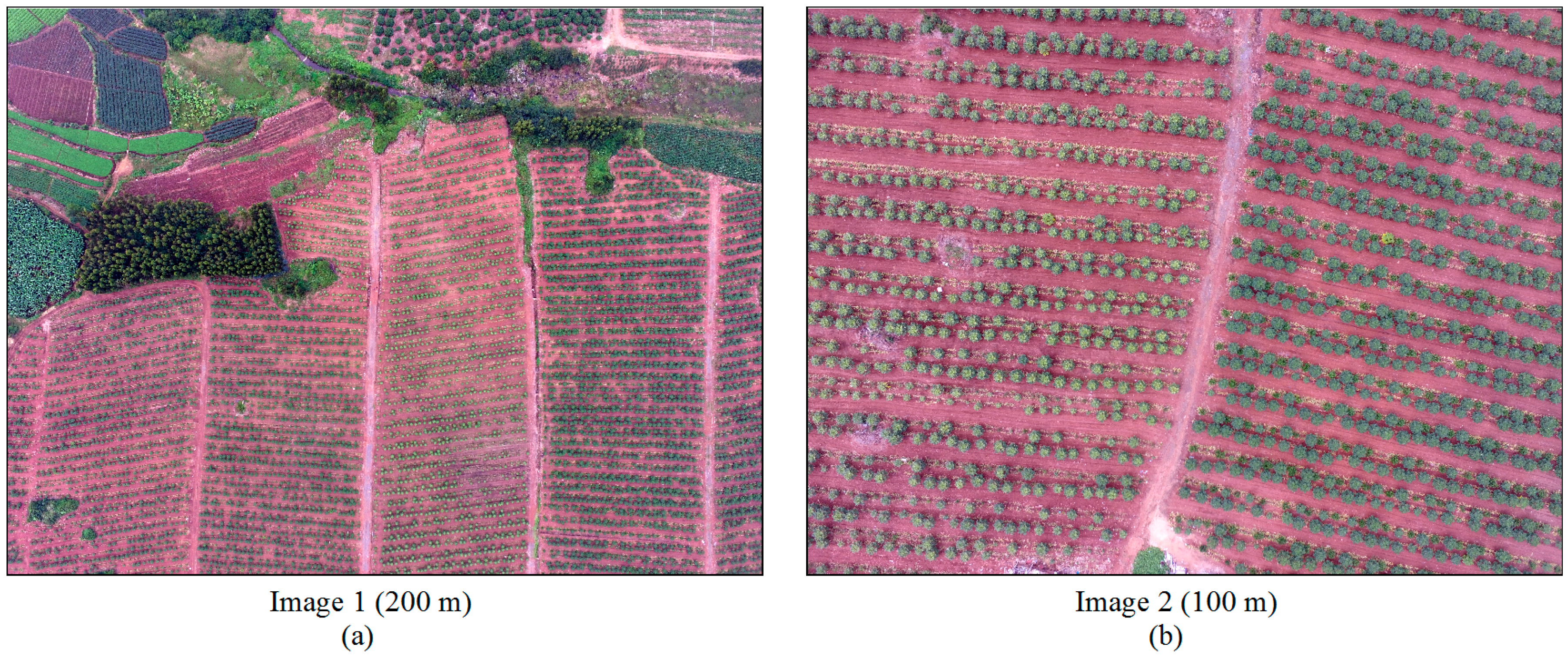
The study area focused on a papaya farm centered at 20.370045°N, 110.056553°E, located in Xuwen County, Zhanjiang City, Guangdong Province, China. The soil in Zhanjiang City is mainly red soil formed by rich minerals [13], and the stands are relatively isolated with many of them intercropping with lemon. Two images, e.g., 1 (Figure 1a) and 2 (Figure 1b) were captured respectively, the image details are listed in Table 1. Both images contain other plants that may cause misidentification, e.g., Image 1 is complex and contains shrubs, eucalyptus, banana, and litchi trees, while Image 2 is simple and contains only an automatic weather station and some shrubs.
2.2. Equipment: Unmanned Aerial Vehicles (UAV) and Computers
The UAV used in our experiment was a Quadcopter (with 4 rotors) called DJI Phantom 3 Professional. It was equipped with a consumer-grade digital camera and the technical details are listed in Table 2. The camera can only take three visible bands of red, green and blue (RGB), while the near-infrared band, commonly used in vegetation analysis [14], is unavailable.
We tested the proposed method on a CPU-GPU heterogeneous computer. The CPU used was an Intel i7-4790 at 3.60 GHz with 8-cores and 16 GB of host memory, and a memory speed of 1.6 GHz with a 64-bit GDDR3 interface. The GPU was an NVIDIA GeForce 1080 GTX running at 1.733 GHz with 2560 compute units, a device memory of 8 GB, a memory speed of 10 Gbps (10.0 GHz effective), and a 256-bit GDDR5X interface. The tests were performed on a 64-bit Ubuntu 16.04 operating system. The versions of GCC, CUDA, and PyCUDA were 4.9.3, 8.0, and 2016.1.1, respectively. Only single-precision floating point numbers were considered in algorithm implementation.
2.3. Validation Data
SSF based tree detection can produce two types of information: the coordinate and radius of the tree crowns. As the tree crowns of papaya and lemon trees appeared small in our captured images, in addition to the geometric deformation of the image, the radius lacks practical value. Thus, the validation only considered the coordinates while the radius was discarded.
In this study, we defined the tree crown coordinate as the center of the tree crown. For each image, two independent student interpreters constructed a reference dataset by manually delineating the coordinates in the image using ArcMap 10.2. The interpreters also participated in our UAV flight mission, thus have basic knowledge regarding the study area. The datasets from two interpreters were cross validated and the uncertain points discussed to enable ground truth data.
It is important to mention that the detected coordinates of the tree crowns may deviate from the ground truth, so point-to-point analysis will lead to mismatches in validation. To avoid this, we set a buffer for each detected coordinate when performing validation, e.g., if a ground truth point was within the buffer of a detected point, it was a correct detection. The buffer was circular and the radius was set as the minimum value of σ (σmin), which is introduced in the following section.
2.4. Scale-Space Filtering (SSF) Based Tree Detection Method
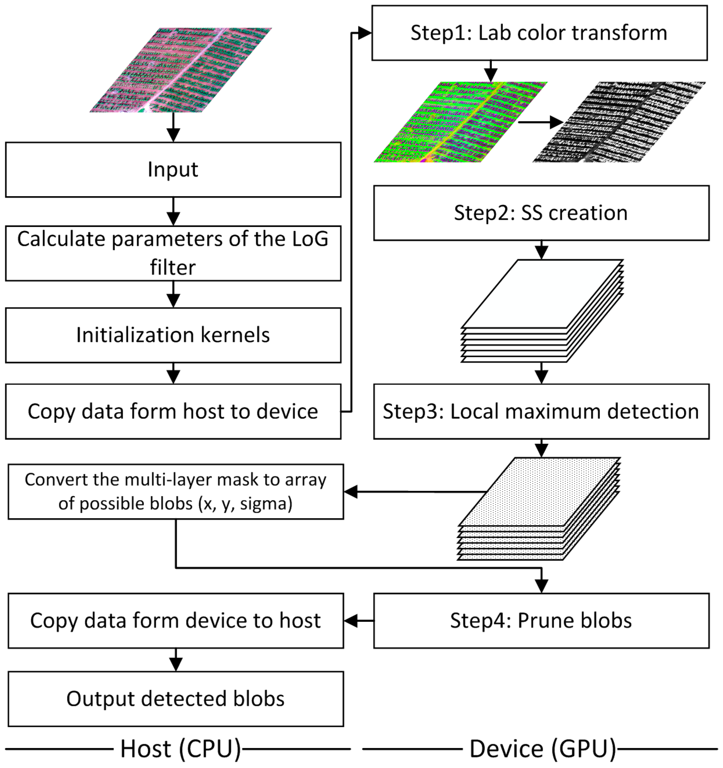
The proposed tree detection method using SSF contained four steps, the details are as follows:
2.4.1. Lab Color Transformation (CT-Lab)
The scale-space was constructed from a single channel grayscale image, which is generally converted from the original RGB image based on transformations including luminous intensity, vegetation indices, or color space [15]. It was essential to choose one that provided high contrast between the trees and backgrounds. The first two methods were closely related to luminance, which may have caused over-detection problems attributable to some small objects appearing as “bright blobs”, including concrete platforms or bare soil. However, these confusing objects differed significantly from papaya and lemon trees in color space. Thus, we transformed the image from the original RGB color space to a Lab color space, which is a color-opponent space with three channels with L for lightness and a (red-green) and b (yellow-blue) for the color-opponent channels [16,17]. Given that the soil in our study area was red and the papaya and lemon treetops were green, the a-channel was very suitable as the grayscale image to construct the SS.
2.4.2. Scale-Space Creation (SSC)
The SS was created as a multi-scale representation of an original intensity image. Blobs of different sizes were highlighted in their corresponding representation scales, which was achieved by convolving the input image with the Gaussian kernel operator (Equation (1)) and the Laplacian operator (Equations (2) and (3)), which facilitated image smoothing and blob sharpening, respectively. In practice, the two operators are often combined and simplified as the Laplacian of Gaussian (LoG) operator (Equation (4)).
2.4.3. Local Maximum Detection (LMD)
The blobs were then detected using local maxima filtering at each scale. A local maximum was defined as a pixel with gray values not only larger than their eight immediate neighbors, but also larger than a specified threshold Tgray. We used the maximum’s location and corresponding σ to represent the blob’s centroid and radius. However, due to the variation in tree structures and sunlit angles, the brightest areas were not always at the centers of the blobs. This may lead to problems where a single blob may be detected over several scales (with varied centroid and radius), thus requiring us to further determine which detection is optimal.
2.4.4. Prune Blobs (PB)
The optimal blob was considered to have the highest response in a small overlapping area (OA) of SS. The OA rate was calculated by circle-to-circle intersection [18]. The process of pruning blobs first involved determining a threshold of OA rate, followed by a comparison of two blobs if their max OA rate exceeded a threshold value. The blob with the higher response in scale was kept, while the other was discarded. This comparison enumerated every two-blob combination.
2.5. Graphics Processing Unit (GPU) Implementation
Conventional multicore CPUs devote more resources to caching or control flow operations. However, within limited chip areas, the GPUs tend to minimize the control logic and memory caches, but enable more computing units for the execution of massive numbers of threads. For example, modern high-performance GPUs such as NVIDIA GeForce GTX1080 provide 2560 computing units, whereas in contrast, the contemporary CPU e.g., Intel i7-6900 contains only eight cores. In this way, scientific computations such as SSF can be accelerated via a CPU–GPU heterogeneous platform in the following way: first, using the host CPU to perform sequential operations including image input/output (I/O) and control operations; and second, using the GPU device to solve the computational and memory-intensive problems.
The compute unified device architecture (CUDA) is a heterogeneous sequential-parallel programming model and software environment that allows for access to the NVIDIA’s GPU resources via so-called kernels. Several programming languages including C/C++, Fortran, and Python are supported for written kernels. Compared to the other non-scripting languages, Python emphasizes quick development and offers a comprehensive mathematics library that has been widely adopted by scientific communities. PyCUDA involves using Python as a wrapper to the CUDA C kernels, and features Python’s automatic memory management, error checking, and requires no user-visible compilation, which makes it very suitable for interactive testing and quick prototyping in our applications.
In this study, the sequential implementation of the SSF algorithm used was based on the Scikit-image package [19] mainly written in Python, where some performance critical sections including color-transform, LoG convolution, and maximum filtering were written in the C programming language (wrapped in SciPy library [9]), while the prune blob process was implemented in ordinary Python. To optimize the performance of the sequential version algorithm, we re-wrote it using Cython [20], which is an optimizing static compiler support near C execution speed with Python code.
To achieve a fair benchmark in terms of execution time with respect to the CPU version, we ported the four most time consuming steps of the algorithm to GPU using PyCUDA, while the other ordinary processes were the same as the sequential task (Figure 2). In the following process, we describe the details of the parallel implementation for each step:
- (1)
- CT-Lab: We used a 32 × 32 window to arrange threads in each block, where each thread performed the RGB to Lab color transformation on a pixel-wise basis. This was due to the maximum number of threads per block being 1024 for our GPU device, and that the 2-dimensional (2-D) arrangement of threads other than 1-D may have reduced the idle threads when processing 2-D images.
- (2)
- SSC: We first calculated the parameters of the LoG operator in the host and then, together with the image, transferred them to the device. The 2-dimensional (2-D) LoG filter was isotropic, and can be separated into two 1-D components (x and y), resulting in a decrease in redundant computations. We used two different kernels to calculate the x and y components and combined them using another kernel. The key point of exploring the power of GPU was using the shared memory, an on-chip cache that operated much faster than the local and global memory. One common problem may appear when the filter window reaches the array border where part of the filter may fall outside the array and will not match corresponding values. This was undertaken by assuming that the arrays were extended beyond their boundaries as per the “reflected” boundary conditions, which involved repeating the nearest array in an inverse order. Other details can be found in previous works since Gaussian-like filtering is one of the most basic applications of CUDA [21].
- (3)
- LMD: We detected the local maximum by filtering the image sequence of SS consecutively through each x, y, and z direction. The over boundary arrays were extended as per the “constant” (repeat a constant value, e.g., zero) instead of “reflected” boundary conditions as the latter may cause over detection in maximum detection. To minimize the time cost in data transfer, only the input image and filtered results were transferred between the host and device, while the intermediate variables were stored in the GPU’s global memory and allocated in advance.
- (4)
- PB: Once the local maxima in SS were identified, the x and y coordinates and σ for each maxima were extracted into an array, which was then transferred to the GPU as the input of the blobs pruning kernel. Our arrangement intended to compare the blobs in a parallel manner over each of the two blob combinations using an associated thread. A three-part algorithm was implemented as follows:
First, an iterative calculation was performed for each thread regarding how to locate its corresponding blobs. For an array S of size n, the number of the two blob combinations was n × (n − 1)/2. We defined icomb as the index for enumerating each of two blob combinations, and p and q as the indexes of corresponding blobs. It was difficult to directly associate a single thread id with two indices (p and q) other than a single index (icomb). Hence, we derived the indices p and q from index (icomb) iteratively using Algorithm 1. Note that a UAV image often contains thousands of trees and may cause even more possible detections, therefore the number of two-blob combinations (Ncomb) may be great enough to exceed the maximum number of available blocks * threads (Nbt). In these cases, there may be a need to execute the kernel by loops, with each loop indexed by iloop processing a subset of Ncomb. It was recommended to set the size of a subset equal to or less than Nbt to achieve optimal performance, since it can coalesce access to memory. The Nbt depended on the GPU architecture and kernel occupancy (registers and local memory), and in our case, the Nbt was equal to on GTX1080.
Second, the OA rate of blob p and q was calculated using the aforementioned algorithm [18], with the only difference being that it was implemented as a device function.
Third, the thread compared two blobs if their max OA rate was larger than the threshold; in this case, the blob with the higher response in scale as kept and the other discarded. These codes were implemented in PyCUDA.
| Algorithm 1. Pseudocode for locating blobs for each thread. |
| 1: INPUTS: index of kernel running (), size of blobs array (n) 2: compute = blockIdx.x * blockDim.x + * Nbt + threadIdx.x + 1 3: define a temporary variable L to store number remains 4: check if (< = 0 or > (n × (n − 1)/2)): True: set p = −1 and return; False: continues 5: set loop starting conditions: p = 1, L = n − p 6: start loop: while ( > L): icomb − = L; p + = 1; L = n − p; 7: Compute indices (p and i): p − = 1; q = p + (); 8: OUTPUT: indices of blobs array (p and q) |
2.6. Metrics for Evaluating Accuracy of Tree Method Detection
To evaluate the performance of our proposed tree detection method quantitatively, three metrics, including precision, recall and F-measure, were calculated by comparing the results with the ground truth:
where true positive (TP) and false positive (FP) are correct and incorrect detections, respectively. False Negative (FN) is the missed detection and α is a non-negative scalar that balances precision and recall. Precision represents the probability that the detections are valid, recall is the probability that trees are correctly detected, and F-measure is the weighted harmonic mean of precision and recall. The α ordinarily takes the values of 0.5, 1, or 2, where it signifies three situations: (1) recall weighs twice as much as precision; (2) precision and recall are equal; and (3) precision weighs twice as much as recall, respectively [22]. In this study, we set α as 0.5 following studies [15,23] that emphasize recall rather than precision.
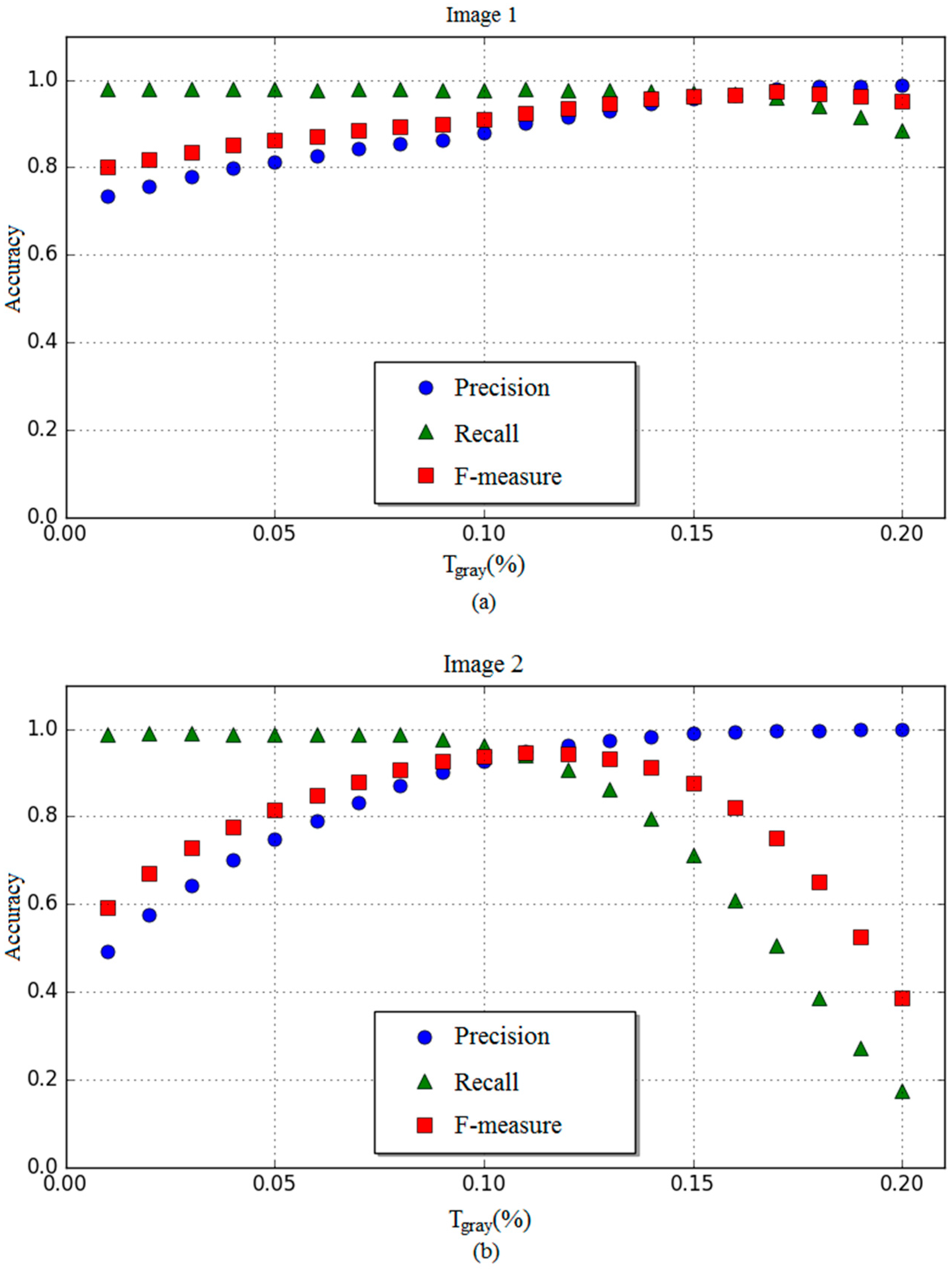
There are five parameters associated with the proposed tree detection method, including σmin, σmax, Nsigma, OA, and Tgray. Among them, the first two can be directly estimated from the image, while the Nsigma and OA are relatively stable. However, Tgray is very sensitive to the accuracy of detection. To explore the potential as much as possible, we tested the proposed method on a range of Tgray (Equation (8)) while other parameters were fixed for each image (Table 3).
where Vmax and Vmin are the maximum and minimum gray values in the image; and c is a variable that ranged from 0.01 to 0.2 in steps of 0.01.
2.7. Metrics for Evaluating Graphics Processing Unit (GPU) Performance
We selected two metrics, e.g., runtime and speedup, for evaluating the GPU performance, and the runtime of both sequential and parallel algorithms were obtained for each image. It should be noted that the reported times were the minimum of ten executions for each running. In addition, the runtime required for each step included the data transfer time from the host to the device memory, and the total time contained the runtime of four steps and all other data processing time, with the exception of data transfers with hard disks.
The speedup was then calculated as the runtime of parallel algorithms executed on the GPU in comparison to its sequential counterpart running on a single core CPU. The same definition of runtime and speedup are used in subsequent discussions.
3. Results and Discussion
3.1. Tree Detection Accuracy
The variation of three assessing metrics based on the change of Tgray is shown in Figure 3. For Image 1, the highest F-measure achieved was 0.942, while the precision was 0.932 and recall was 0.963. For Image 2, the highest F-measure was 0.960, precision was 0.954, and recall was 0.973.
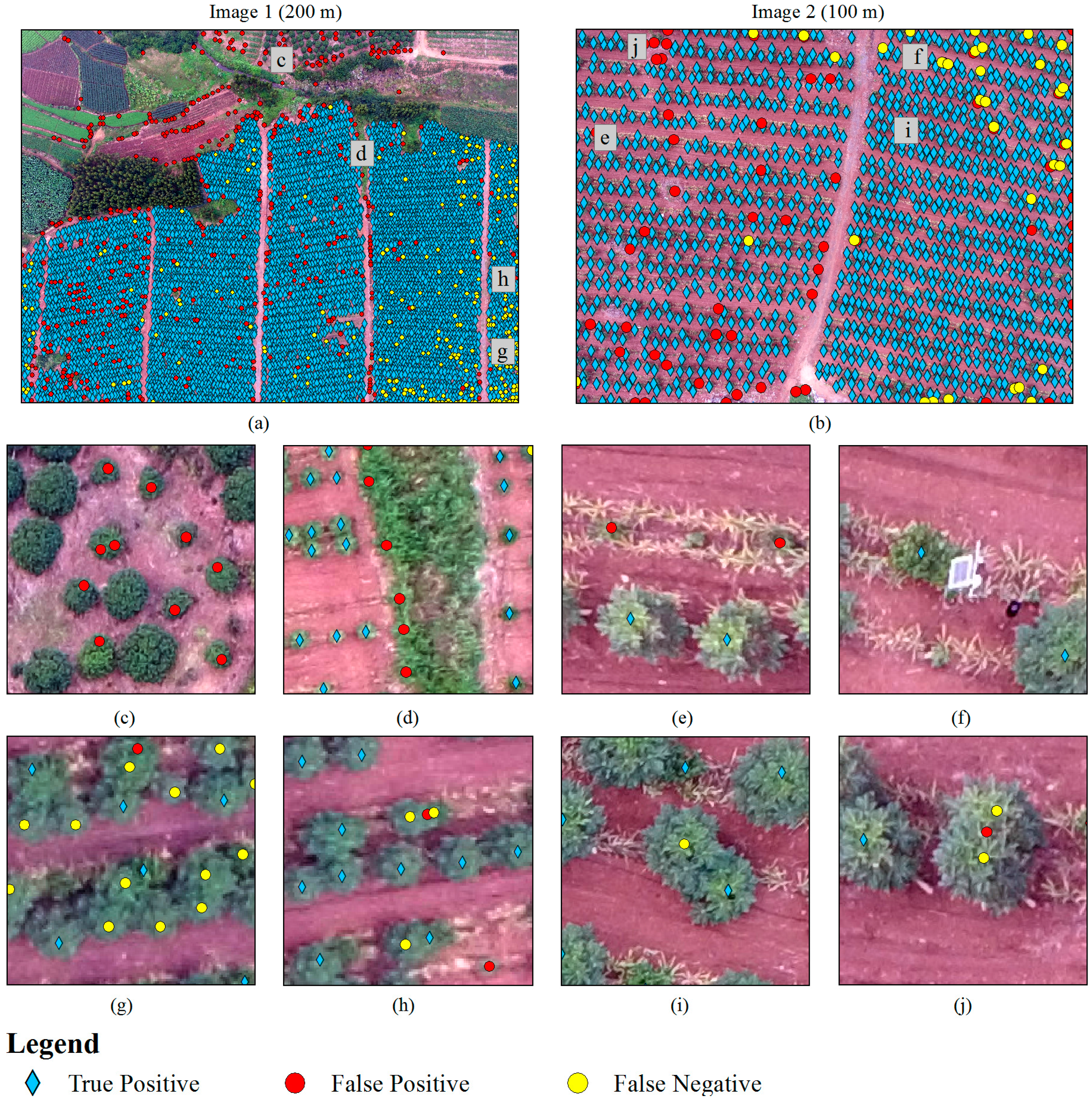
It is worth mentioning that as per the highest F-measure associated parameters, there were 7640 and 1476 possible trees detected for the two images, respectively through Step 3: LMD; after performing blob pruning, 7565 and 1354 were retained as tree detection results, respectively (Table 4).
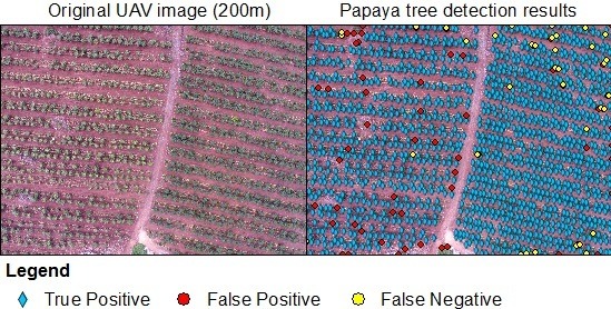
The associated results are illustrated in Figure 4a–j. Among them, Figure 4a,b are the tree detection results overlaid the original images. The false positives were mainly attributable to improper detection of litchi trees (Figure 4c), shrubs (Figure 4d), or dead papaya trees (Figure 4e). Note that an automatic weather station appeared as bright in Image 2, and may have been over-detected under luminance-based methods, but was not detected in the proposed method (Figure 4f). The false negatives were mainly caused by the misidentification of the overlapping canopies of trees, and was attributed to two situations: (1) a camera-induced blur on the edges of an image that may have reduced contrast between the canopy and the background, thus resulting in misidentification (Figure 4g) mostly occurring in the right bottom corner of Image 1 (Figure 4a); and (2) two nearby trees that were misidentified as one (Figure 4h–j).
In this study, the SSF based tree detection method achieved high F-measure. The reason may be due to the fact that the papaya farm in our study area was a relatively sparse forest, which was within the scope of the method. However, the drawbacks of the SSF based tree detection method are that it may result in low performance for dense forest, which is why incorrect detections in this study mainly occurred in overlapping trees where nearby trees were misidentified as one. Previous studies have indicated that among the several tree detection methods, there was no method able to handle all types of forests [10]. Thus for dense tree detection, it is highly recommended that suitable methods e.g., deep learning based [9] are selected over the SSF based method.
In addition, the SSF method blurred the image using a Gaussian filter with several σ, and detected possible trees in each blurred layer. However, if an image was already blurred, the large trees could still be detected while the small trees may be ignored. Furthermore, if the blur mixed nearby tree crowns, the performance of tree detection was reduced. There were some common issues that may have caused the low-quality image of the UAV, including motion blur or camera unforces. Although there are methods that can enhance the quality of the image [24]; it was essential to arrange the flight campaign under good conditions e.g., good weather, appropriate camera adjustment, flight speed, and flight altitude [14].
The two images were captured under similar conditions including weather, ground and the use of the same UAV, with the only difference being flight height. However, for the highest F-measure of each image, the associated variable of c (in parameter Tgray) was 0.17 and 0.11 respectively. In addition, for Image 2, the values of c, other than 0.11, resulted in a significant reduction in f-measure. This emphasized that the parameter of Tgray was very sensitive and required careful tuning; however, in practice, there is no ground truth for its optimization. In this way, a trial-and-error process is often necessary for choosing the appropriate parameter set interactively. Thus, there is a great need for executing the algorithm rapidly.
3.2. GPU Performance
It can be seen in Table 5 that the runtimes of the other processing steps were very close (nearly 46 ms); however, the runtime of the four steps varied significantly. For sequential implementation, they were 44,372.72 ms and 23,858.35 ms; and for parallel implementation, they were 945.45 ms and 790.92 ms. The total speedup achieved by our parallel implementation was 44.77 and 28.54 for the two images.
Step 1 was a Lab color transform, and the runtime of the two images were similar for both sequential and parallel algorithms as the Lab color transform used fixed parameters in both images. The situation was similar to Step 3 (LMD). However, the speedups achieved using Step 1 were larger than those associated with Step 3, mainly because Step 1 took advantage of GPU performance for floating point calculations, but computational intensity was low in Step 3 as its filter radius was only 1.
Step 2 was SSC where the speedup differed for the two images. Image 2 required more time than Image 1 for sequential algorithms, but their runtimes were similar for the parallel algorithm. The reason behind this was that the runtime of the LoG filtering was largely determined by the filter radius. The filter was much smaller for Image 1 (ranging from 12–24, which was four times σ) than for Image 2 (ranging from 60–100). In contrast, the parallel algorithms utilizing the shared memory of the GPU to store temporary data and the data access time were negligible, which showed that the filter radius had little effect on the runtime of the parallel algorithms.
Step 4 consisted of pruning blobs. The runtime of the two images differed considerably between sequential and parallel algorithms. The computational intensity in the two images differed by a factor of almost 31 times. Given that there were 7640 possible trees in Image 1 (7565) and 1476 trees in Image 2 (1354), the number of two-blob combinations in Image 1 was 31 times greater than in Image 2. Due to the high degree of parallelism of the GPU, the parallel algorithm achieved the most significant speedup at more than 218 times that of the sequential algorithm.
To conclude, due to the different quantities and sizes of papaya and lemon trees in the two images, the benefits of the GPU became more significant for Steps 1, 2, and 4 as they involve floating point calculations and convolution operations. As described previously, the optimal parameters varied depending on the characteristics of the image, such as view-altitude and species mixture. In this way, a trial-and-error process was often necessary in selecting the appropriate parameter set. With the help of GPU, the total runtime for both images were reduced from an average of 34 s to less than 1 s, which achieved a real-time response that may support swift parameter optimization and image analysis.
Furthermore, it is worth mentioning that the total runtime could be further accelerated. As the four steps of the proposed method are designed as separate modules, each module contains the data transfer of host-to-device and device-to-host. This design facilitated the comparison with sequential algorithm, but resulted in wasted time in data transfer between the intermediate modules. In our proposed method, there were no sequential operations required between Steps 1, 2, and 3. The former three modules could be combined where the intermediate data was retained on the device to reduce unnecessary data I/O. However, the only exception was that it required a sequential operation to convert local maxima from a 3-D matrix (the output of Step 3) to an array (the input of Step 4), thus Step 4 was still an independent module.
Tree detection is a time-consuming application. In addition, the sum of the algorithm runtime was often greater than linear increases in image size, especially for algorithms requiring global optimization (e.g., MRF and MPP). Therefore, previous studies have generally used small images less than 600 pixels in width, despite cases of running on similar CPUs where the runtime was often more than 20 minutes [8]. Considering that UAV cameras continue to improve, their accessibility for more research groups has grown, that image size and quantity are increasing, and the demand for fast algorithm is more intense, our proposed method is expected to be used more widely.
4. Conclusions
In this paper, we proposed a tree detection method for UAV images based on GPU-accelerated scale-space filtering. The parallel implementation was specifically tailored to large images, taking advantage of the GPU architecture. This approach included separated filter kernels, using shared memory to ensure coalesced memory access, and indexed two-blob combinations iteratively to enable massive parallel floating-point calculations.
Two consumer-grade UAV images containing papaya and lemon trees of different crown sizes were evaluated. Our results indicated significant accuracy with an F-measure larger than 0.94. The speedup achieved by our parallel implementation was 44.77 and 28.54 for both images, respectively, when compared with sequential counterpart. For each image with a size of 4000 × 3000 pixels, the required total runtime was within 1 s of achieving a real-time performance, which is appealing for interactive parameter optimization and application on a large number of images. Future works will explore methods for feature analysis and other tree species identification.
Acknowledgments
This work was jointly supported by the National Natural Science Foundation of China (No. 41601481), Guangdong Innovative and Entrepreneurial Research Team Program (2016ZT06D336), the Natural Science Foundation of Guangdong Academy of Sciences (QNJJ201601), the Science and Technology Planning Project of Guangdong Province (2016A020210060), and GDAS’ Special Project of Science and Technology Development (2017GDASCX-0101).
Author Contributions
Hao Jiang proposed and implemented the method, designed the experiments and drafted the manuscript. Shuisen Chen provided overall guidance to the project and edited the manuscript. Dan Li contributed to the improvement of the proposed method. Chongyang Wang and Ji Yang assisted in the experimental design.
Conflicts of Interest
The authors declare no conflict of interest.
References
- Puliti, S.; Olerka, H.; Gobakken, T.; Næsset, E. Inventory of small forest areas using an unmanned aerial system. Remote Sens. 2015, 7, 9632–9654. [Google Scholar] [CrossRef]
- Gebreslasie, M.T.; Ahmed, F.B.; Van Aardt, J.A.N.; Blakeway, F. Individual tree detection based on variable and fixed window size local maxima filtering applied to ikonos imagery for even-aged eucalyptus plantation forests. Int. J. Remote Sens. 2011, 32, 4141–4154. [Google Scholar] [CrossRef]
- Hirschmugl, M.; Ofner, M.; Raggam, J.; Schardt, M. Single tree detection in very high resolution remote sensing data. Remote Sens. Environ. 2007, 110, 533–544. [Google Scholar] [CrossRef]
- Karlson, M.; Reese, H.; Ostwald, M. Tree crown mapping in managed woodlands (parklands) of semi-arid west africa using worldview-2 imagery and geographic object based image analysis. Sensors 2014, 14, 22643–22669. [Google Scholar] [CrossRef] [PubMed]
- Malek, S.; Bazi, Y.; Alajlan, N.; Alhichri, H. Efficient framework for palm tree detection in uav images. IEEE J. Sel. Top. Appl. Earth Obs. Remote Sens. 2014, 7, 4692–4703. [Google Scholar] [CrossRef]
- Larsen, M.; Rudemo, M. Optimizing templates for finding trees in aerial photographs. Pattern Recognit. Lett. 1998, 19, 1153–1162. [Google Scholar] [CrossRef]
- Descombes, X.; Pechersky, E. Tree Crown Extraction Using a Three State Markov Random Field; INRIA: Paris, France, 2006; pp. 1–14. [Google Scholar]
- Jia, Z.; Proisy, C.; Descombes, X.; Maire, G.L.; Nouvellon, Y.; Stape, J.L.; Viennois, G.; Zerubia, J.; Couteron, P. Mapping local density of young eucalyptus plantations by individual tree detection in high spatial resolution satellite images. For. Ecol. Manag. 2013, 301, 129–141. [Google Scholar]
- Li, W.; Fu, H.; Yu, L.; Cracknell, A. Deep learning based oil palm tree detection and counting for high-resolution remote sensing images. Remote Sens. 2017, 9, 22. [Google Scholar] [CrossRef]
- Larsen, M.; Eriksson, M.; Descombes, X.; Perrin, G.; Brandtberg, T.; Gougeon, F.A. Comparison of six individual tree crown detection algorithms evaluated under varying forest conditions. Int. J. Remote Sens. 2011, 32, 5827–5852. [Google Scholar] [CrossRef]
- Lindeberg, T. Feature detection with automatic scale selection. Int. J. Comput. Vis. 1998, 30, 79–116. [Google Scholar] [CrossRef]
- Ckner, A.; Pinto, N.; Lee, Y.; Catanzaro, B.; Ivanov, P.; Fasih, A. Pycuda and pyopencl: A scripting-based approach to gpu run-time code generation. Parallel Comput. 2011, 38, 157–174. [Google Scholar]
- Zhu, Z.; Xu, Y.; Wen, Q.; Pu, Z.; Zhou, H.; Dai, T.; Liang, J.; Liang, C.; Luo, S. The stratigraphy and chronology of multicycle quaternary volcanic rock-red soil sequence in Leizhou Peninsula, South China. Quat. Sci. 2001, 21, 270–276. [Google Scholar]
- Walczykowski, P.; Kedzierski, M. Imagery Intelligence from Low Altitudes: Chosen Aspects. In Proceedings of the XI Conference on Reconnaissance and Electronic Warfare Systems, Oltarzew, Poland, 21 November 2016. [Google Scholar]
- Srestasathiern, P.; Rakwatin, P. Oil palm tree detection with high resolution multi-spectral satellite imagery. Remote Sens. 2014, 6, 9749–9774. [Google Scholar] [CrossRef]
- Ford, A.; Roberts, A. Colour Space Conversions. Available online: http://sites.biology.duke.edu/johnsenlab/pdfs/tech/colorconversion.pdf (accessed on 17 May 2017).
- Ford, A. Colour Space Conversions; Westminster University: London, UK, 1998. [Google Scholar]
- Weisstein, E.W. Circle-Circle Intersection. Available online: http://mathworld.wolfram.com/Circle-CircleIntersection.html (accessed on 17 May 2017).
- Walt, S.V.D.; Schönberger, J.L.; Nuneziglesias, J.; Boulogne, F.; Warner, J.D.; Yager, N.; Gouillart, E.; Yu, T.; Contributors, T.S. Scikit-image: Image processing in python. PeerJ 2014, 2, e453. [Google Scholar] [CrossRef] [PubMed]
- Behnel, S.; Bradshaw, R.; Citro, C.; Dalcin, L.; Seljebotn, D.S.; Smith, K. Cython: The best of both worlds. Comput. Sci. Eng. 2010, 13, 31–39. [Google Scholar] [CrossRef]
- Liu, J. Comparation of several cuda accelerated gaussian filtering algorithms. Comput. Eng. Appl. 2013, 49, 14–18. [Google Scholar]
- He, H.; Ma, Y. Imbalanced Learning: Foundations, Algorithms, and Applications; John Wiley & Sons, Inc: Hoboken, NJ, USA, 2013. [Google Scholar]
- Martin, D.R.; Fowlkes, C.C.; Malik, J. Learning to detect natural image boundaries using local brightness, color, and texture cues. IEEE Comput. Soc. 2004, 26, 530–549. [Google Scholar] [CrossRef] [PubMed]
- Kedzierski, M.; Wierzbicki, D. Methodology of improvement of radiometric quality of images acquired from low altitudes. Measurement 2016, 92, 70–78. [Google Scholar] [CrossRef]
Figure 1.
Two unmanned aerial vehicles (UAV) images used in this study. Image 1 and 2 were captured at the same orchard, but without spatial overlaps. (a) Image 1 (captured at an altitude of 200 m); and (b) Image 2 (captured at an altitude of 100 m).
Figure 1.
Two unmanned aerial vehicles (UAV) images used in this study. Image 1 and 2 were captured at the same orchard, but without spatial overlaps. (a) Image 1 (captured at an altitude of 200 m); and (b) Image 2 (captured at an altitude of 100 m).

Figure 2.
Summary of the tree detection method based on a parallel implementation of the scale-space (SS) filter.
Figure 2.
Summary of the tree detection method based on a parallel implementation of the scale-space (SS) filter.

Figure 3.
Accuracy of the tree detection results with the variation of parameter Tgray. The precision, recall and F-measure for (a) Image 1; and Image 2 (b).
Figure 3.
Accuracy of the tree detection results with the variation of parameter Tgray. The precision, recall and F-measure for (a) Image 1; and Image 2 (b).

Figure 4.
Tree detection results of the two images, (a) and (b) are tree detection results overlaid on the original images. The false positives were mainly attributable to the improper detection of litchi trees (c); shrubs (d); or dead papaya trees (e). An automatic weather station appeared bright in Image 2, which may have been over-detected under luminance-based methods, but was not detected in the proposed method (f). The false negatives can be attributed to two situations: one is a camera-induced blur on the edges of an image which may have reduced the contrast between the canopy and the background, resulting in misidentification (g); the other was two nearby trees that were misidentified as one (h), (i) and (j).


Table 1.
Information of the two images.
| Information | Image 1 | Image 2 |
|---|---|---|
| Date | 20 December 2015 | 20 December 2015 |
| Local Time | 10:53 | 12:30 |
| Latitude (°N) | 20.3693 | 20.3694 |
| Longitude (°E) | 110.0553 | 110.0574 |
| Flight altitude (m) | 200 | 100 |
| View angle (°) | 0 | 0 |
| Tree (papaya and lemon) numbers of ground truth | 7327 | 1328 |
Table 2.
Imaging sensor specifications.
| Camera Parameters | Values |
|---|---|
| Sensor | Sony EXMOR 1/2.3″ CMOS |
| Effective pixels | 12.4 M (total pixels: 12.76 M) |
| Sensor size | 6.16 mm wide, 4.62 mm high |
| Lens | FOV 94° 20 mm (35 mm format equivalent) f/2.8 focus at ∞ |
| ISO range | 100–1600 (photo), 100–3200 (video) |
| Electronic Shutter Speed | 8–1/8000 s |
| Image Size | 4000 × 3000 |
Note: ISO stands for International Standards Organization, and it is a standardized industry scale for measuring sensitivity of a digital image sensor to light.
Table 3.
Parameters of SSF based tree detection method for two image tests.
| Parameters | Usage | Image 1 | Image 2 |
|---|---|---|---|
| σmin | Minimum value of σ | 3 | 15 |
| σmax | Maximum value of σ | 6 | 25 |
| Nsigma | Number of scale-space | 5 | 5 |
| OA | Threshold of overlapping area ratio | 0.2 | 0.2 |
Table 4.
Performance of Step 4: Prune blobs.
| Processing Step | Image 1 | Image 2 |
|---|---|---|
| Before PB | 7640 | 1476 |
| After PB | 7565 | 1354 |
Table 5.
Runtime and speedup of the proposed method.
| Images | Main Computation Device | Step 1 | Step 2 | Step 3 | Step 4 | Kernel | Total Time (ms) |
|---|---|---|---|---|---|---|---|
| CT-Lab | SSC | LMD | PB | Initialize | |||
| Time (ms) | Time (ms) | Time (ms) | Time (ms) | Time (ms) | |||
| 1 | CPU | 5137.60 | 4175.34 | 1398.84 | 33,660.95 | / | 44,418.80 |
| GPU | 157.67 | 308.92 | 149.51 | 154.22 | 175.13 | 992.22 | |
| Speedups | 32.58 | 13.52 | 9.36 | 218.26 | / | 44.77 | |
| 2 | CPU | 5086.84 | 16,338.77 | 1313.11 | 1119.63 | / | 23,905.13 |
| GPU | 153.05 | 317.89 | 137.60 | 3.97 | 178.41 | 837.62 | |
| Speedups | 33.24 | 51.40 | 9.54 | 282.02 | / | 28.54 |
© 2017 by the authors. Licensee MDPI, Basel, Switzerland. This article is an open access article distributed under the terms and conditions of the Creative Commons Attribution (CC BY) license (http://creativecommons.org/licenses/by/4.0/).
Share and Cite
MDPI and ACS Style
Jiang, H.; Chen, S.; Li, D.; Wang, C.; Yang, J. Papaya Tree Detection with UAV Images Using a GPU-Accelerated Scale-Space Filtering Method. Remote Sens. 2017, 9, 721. https://doi.org/10.3390/rs9070721
AMA Style
Jiang H, Chen S, Li D, Wang C, Yang J. Papaya Tree Detection with UAV Images Using a GPU-Accelerated Scale-Space Filtering Method. Remote Sensing. 2017; 9(7):721. https://doi.org/10.3390/rs9070721
Chicago/Turabian StyleJiang, Hao, Shuisen Chen, Dan Li, Chongyang Wang, and Ji Yang. 2017. "Papaya Tree Detection with UAV Images Using a GPU-Accelerated Scale-Space Filtering Method" Remote Sensing 9, no. 7: 721. https://doi.org/10.3390/rs9070721
Note that from the first issue of 2016, this journal uses article numbers instead of page numbers. See further details here.