Article

Terrestrial Remote Sensing of Snowmelt in a Diverse High-Arctic Tundra Environment Using Time-Lapse Imagery

by
Daniel Kępski
1,*,
Bartłomiej Luks
1,
Krzysztof Migała
2,
Tomasz Wawrzyniak
1,
Sebastian Westermann
3 and
Bronisław Wojtuń
4
1
Institute of Geophysics, Polish Academy of Sciences, Księcia Janusza 64, 01-452 Warsaw, Poland
2
Department of Climatology and Atmosphere Protection, University of Wroclaw, Kosiby 8, 54-621 Wrocław, Poland
3
Department of Geosciences, University of Oslo, Postboks 1047 Blindern, 0316 Oslo, Norway
4
Department of Ecology, Biogeochemistry and Environmental Protection, University of Wroclaw, Kanonia 6/8, 50-328 Wrocław, Poland
*
Author to whom correspondence should be addressed.
Remote Sens. 2017, 9(7), 733; https://doi.org/10.3390/rs9070733
Submission received: 24 April 2017 / Revised: 27 June 2017 / Accepted: 12 July 2017 / Published: 15 July 2017
(This article belongs to the Special Issue Snow Remote Sensing)

Abstract

:
Snow cover is one of the crucial factors influencing the plant distribution in harsh Arctic regions. In tundra environments, wind redistribution of snow leads to a very heterogeneous spatial distribution which influences growth conditions for plants. Therefore, relationships between snow cover and vegetation should be analyzed spatially. In this study, we correlate spatial data sets on tundra vegetation types with snow cover information obtained from orthorectification and classification of images collected from a time-lapse camera installed on a mountain summit. The spatial analysis was performed over an area of 0.72 km2, representing a coastal tundra environment in southern Svalbard. The three-year monitoring is supplemented by manual measurements of snow depth, which show a statistically significant relationship between snow abundance and the occurrence of some of the analyzed land cover types. The longest snow cover duration was found on “rock debris” type and the shortest on “lichen-herb-heath tundra”, resulting in melt-out time-lag of almost two weeks between this two land cover types. The snow distribution proved to be consistent over the different years with a similar melt-out pattern occurring in every analyzed season, despite changing melt-out dates related to different weather conditions. The data set of 203 high resolution processed images used in this work is available for download in the supplementary materials.

Graphical Abstract

1. Introduction

In Arctic tundra landscapes, the distribution and abundance of plants are strongly influenced by the snow cover and its duration [1,2]. In this region, plant growth takes place in the relatively short summer season. Snow cover reduces the amount of light available for photosynthesis, dominates the thermal balance of the ground, and controls the amount of liquid soil moisture [3]. Overall, a number of studies have documented the influence of snow cover duration and its depth to plant phenology and growth in the Arctic [4,5,6,7].
Despite a generally good understanding of the complex relationships between snow cover and vegetation, it is hard to predict plant responses to changes in the amount of snow in a warming climate [6,8,9], which in turn influence processes in the whole ecosystem [10]. Therefore, ecology studies require spatial data sets of snow cover properties [11], in particular for long-term monitoring.
In arctic regions like the Svalbard archipelago, wind redistribution of snow within the micro-relief of the landscape makes the snow cover very heterogeneous [12]. Additionally, the duration of the snow-free period is short, lasting typically from the beginning of July until the end of September [13,14]. This means that even small variations in snow cover duration can influence vegetation development. Therefore, correlations between snow cover and vegetation should be analyzed spatially, making remote sensing methods indispensable tools. Larger-scale vegetation studies based on satellite data are scarce [15,16,17,18] and often problematic due to frequent cloudiness and low frequency of image acquisition, which prevents observing short-term (e.g., daily) and in many cases even seasonal changes in snow cover extent (SCE). On more local scales, automatic time-lapse cameras offer the possibility to overcome such problems and provide both a high temporal and spatial resolution, largely independent of cloudiness. Even unprocessed images from cameras can provide useful data, e.g., for evaluating snow depths from stakes [19,20] and the extent of the snow cover [21], for specifying the state of falling precipitation, for estimating snow interception by tree canopies, or to assess and quantify surface albedo [20]. If the images can be orthorectified and georeferenced, further spatial analyses become feasible. This allows a direct comparison with other georeferenced spatial datasets, such as vegetation maps or terrain properties (slope, aspect, etc.) derived from digital elevation models (DEMs). The advantages of such an approach have been demonstrated in a number of studies in the Arctic region [22,23,24,25]. With its steep mountainous terrain, Svalbard offers excellent possibilities to install time-lapse camera systems on exposed slopes that facilitate monitoring of snow cover and melt dynamics over relatively large areas. Although the Arctic is getting more accessible [26], harsh conditions (freezing temperatures, strong wind) make field measurement campaigns an expensive, time-consuming and potentially dangerous task [27]. However, automatic camera systems require only minimal maintenance which makes them well suited for Arctic conditions. Data sets of high spatial and temporal resolution derived from camera images can be used for both validating [28,29] and enhancing the quality of satellite-derived snow cover observations with lower resolution [30]. Furthermore, SCE maps obtained from time-lapse imagery are valuable in a range of scientific applications, because snow is crucial for seasonal albedo changes [31], heat fluxes between the air and the ground surface [32,33,34], and the thermal regime of the ground [35,36,37]. Ground-truthed SCE information can also be used to enhance climate modelling [38,39], although many models do not take into account the small-scale distribution of the snow cover [40].
The main objective of this work is to analyze the snow cover evolution during the melting period, and its relationship to different vegetation types in the tundra environment of southern Spitsbergen. In this work, we present and evaluate a data set of high-resolution daily SCE maps from high-arctic tundra in southern Svalbard based on automatic time-lapse imagery. We first present details on the camera set-up, the image orthorectification and SCE processing scheme, as well as on data availability. Furthermore, we analyze the snow cover evolution during the melt period for three consecutive melt seasons, with a focus on the interannual variability of the melt-out patterns and on correlations with the occurrence of different vegetation types. Our research hypothesis assumes that the snowmelt pattern is repetitive every year and reflects the occurrence of specific plant communities.

2. Materials and Methods
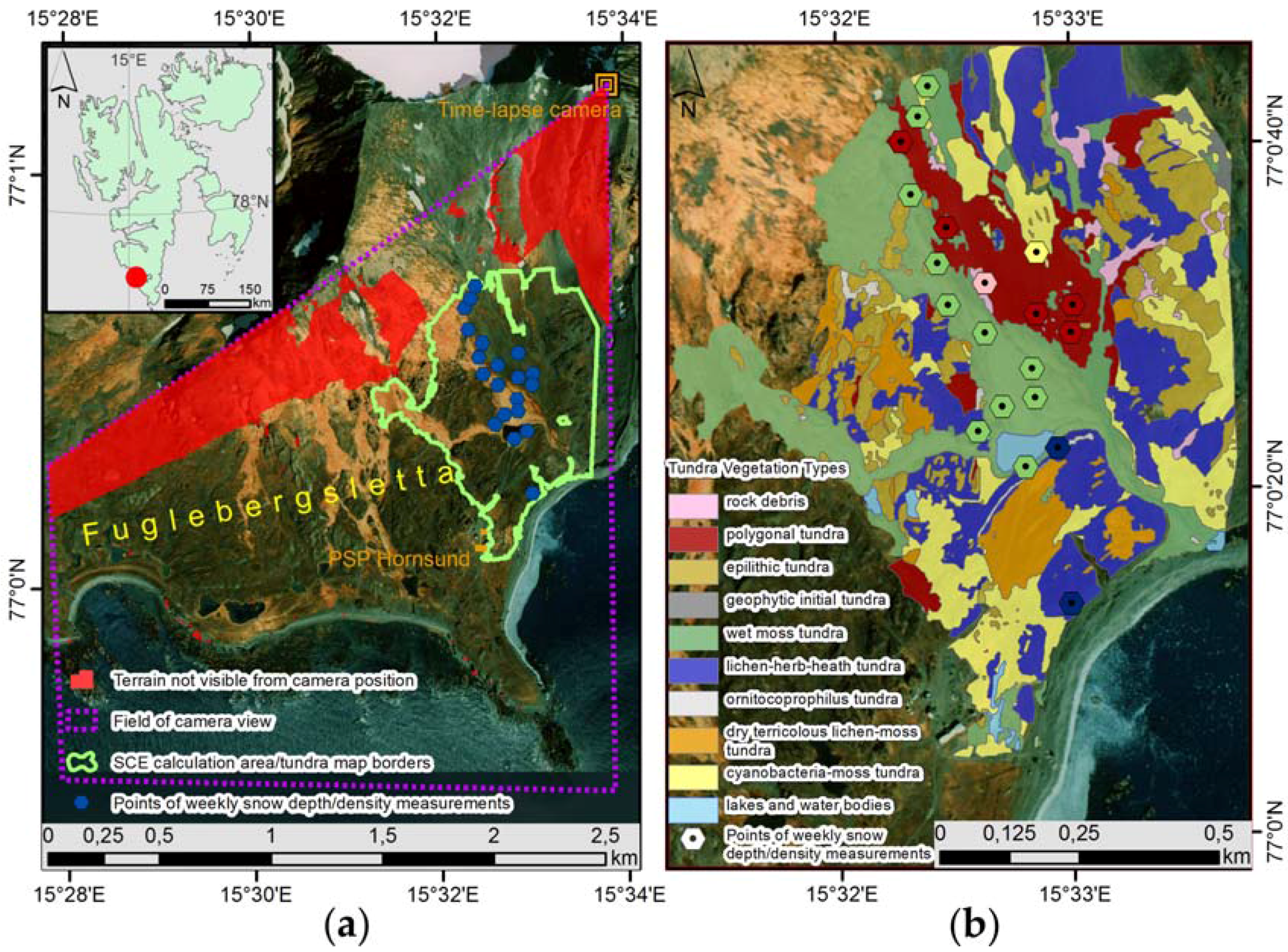
2.1. Study Area

The study was carried out in the vicinity of the Polish Polar Station (PPS) in Hornsund fjord, Spitsbergen, Svalbard (Figure 1). The area represents an unglaciated coastal environment with tundra vegetation which comprise only a small fraction of Svalbard’s land area [15]. The study was conducted in the lower Fuglebekken (“bird stream”) catchment (~1.5 km2) which is a part of the larger Fuglebergsletta plain, a raised marine terrace [41].
For this study, we restrict the investigated area to the lower part of the catchment (0.72 km2). The mean altitude is 16 m a.s.l., with slightly higher terrain towards the north, up to an elevation of 54 m a.s.l. at the highest point at the foothill of the Fugleberget-Ariekammen ridge.
The continuous activity of the Polish Polar Station since 1978 provides an excellent climatological background for the coastal area of Hornsund. The meteorological record (WMO station No. 01003) shows an average air temperature of −4.3 °C and average total precipitation of 435 mm [43], of which as much as 60% falls as snow or sleet [44]. On average, the snow cover on the Fuglebergsletta plain occurs for 244 days of the year and reaches a maximum depth of 43 cm at the end of April [43]. However, both snow depths and duration vary strongly from year to year [14]. Moreover, the snow cover is continuously modified by wind drift, mostly caused by a strong easterly wind [45]. The snow-free period usually lasts from July to September. In the entire climatological record, only 9 days in July/August and 15 days in September were noted as days with snow cover on the ground [43].
Between 2014 and 2016, the study area experienced a wide range of weather conditions (Table 1). The highest snow depth was noted in spring 2014, when maximum accumulation occurred in May, i.e., about one month later than normal. All three winter seasons were significantly warmer in comparison to long-term averages. The winter season 2015/16 was especially warm, with positive temperatures already dominating in May. Although the years 2014–2016 deviate from the multiannual norm in terms of temperature, the year 2013/14 can be considered as snow-rich. As the climate in Svalbard is warming rapidly [46,47], winters with average or cold conditions are increasingly less likely, so that the results from 2014–2016 are highly relevant in the context of the changing Arctic climate.
In the study area, ten different land cover classes are distinguished with respect to plant species [42,48]. More than half of the area is occupied by two classes (Figure 1b): wet moss tundra (26.2% coverage) occurs in conjunction with the wettest hyperskeletic cryosol soil type, and lichen-herb-heath tundra (24.2%) is linked to the driest haplic cryosol type [48,49]. In the Fuglebekken area, dry lichen-herb-heath tundra (Figure 1b) covers flat and exposed areas. Wet moss tundra is the only wet type of tundra here, occupying the close vicinity of the Fuglebekken stream, while all other types are considered as dry plants communities. Cyanobacteria-moss tundra (15.4%) is defined by species that are associated with a long-lasting snow cover (snowbed communities) [50,51,52]. This habitat types covers small patches in the study area, predominantly close to rocky outcrops (Figure 1). Cyanobacteria-moss tundra in the Fuglebekken area is characterized by sparse occurrence of vascular plants, while mosses and cyanobacteria dominate [52]. In general, the study area is characterized by rich vegetation in comparison to other locations in Svalbard [53], mostly due to the presence of large bird colonies [54,55] fertilizing the otherwise nutrient-limited tundra sites.

2.2. Data

Meteorological parameters were obtained from the Hornsund station records (Table 1), operated according to WMO standards [56]. At the station, the snow depth is measured every day at three points at a distance of approximately 50 m from the building on its leeward (western) side. Information about snow depth and density in the Fuglebekken catchment was provided from measurements managed by PPS personnel. These measurements started in 2013 as an additional snow monitoring program and comprise a weekly survey of 20 points when a continuous snow cover is present on the ground (first observations made on 28 October 2013; 20 October 2014; 21 November 2015). The depth is read from snow stakes (installed in 2013), while the average density and the snow water equivalent (SWE) are measured by weighing snow samples obtained with a 60 cm long tube close to the stakes. The data collection depended on weather conditions which resulted in extended gaps between measurements during period of unfavorable weather. The measurements were generally performed until the snow had completely disappeared from the location of the point. However, due to melt ponds during intense ablation, the depth and density assessment often ended earlier (14 June 2014; 24 May 2015; 3 June 2016).
In this work, a set of maps and GIS materials created during previous studies was used. The DEM employed for orthorectification was downloaded from Norwegian Polar Institute resources [57] and rescaled from its native resolution of 20 m to 1 m. The orthophotomap by Kolondra [58] served as a reference to correct the georeferencing of the obtained orthorectified photos. The georeferencing accuracy was additionally evaluated using Landsat 8 panchromatic scenes for days that coincided with time-lapse photo acquisition. Vegetation data were derived from a map of tundra vegetation types published in Migała et al. 2014 [48].

2.3. Methods

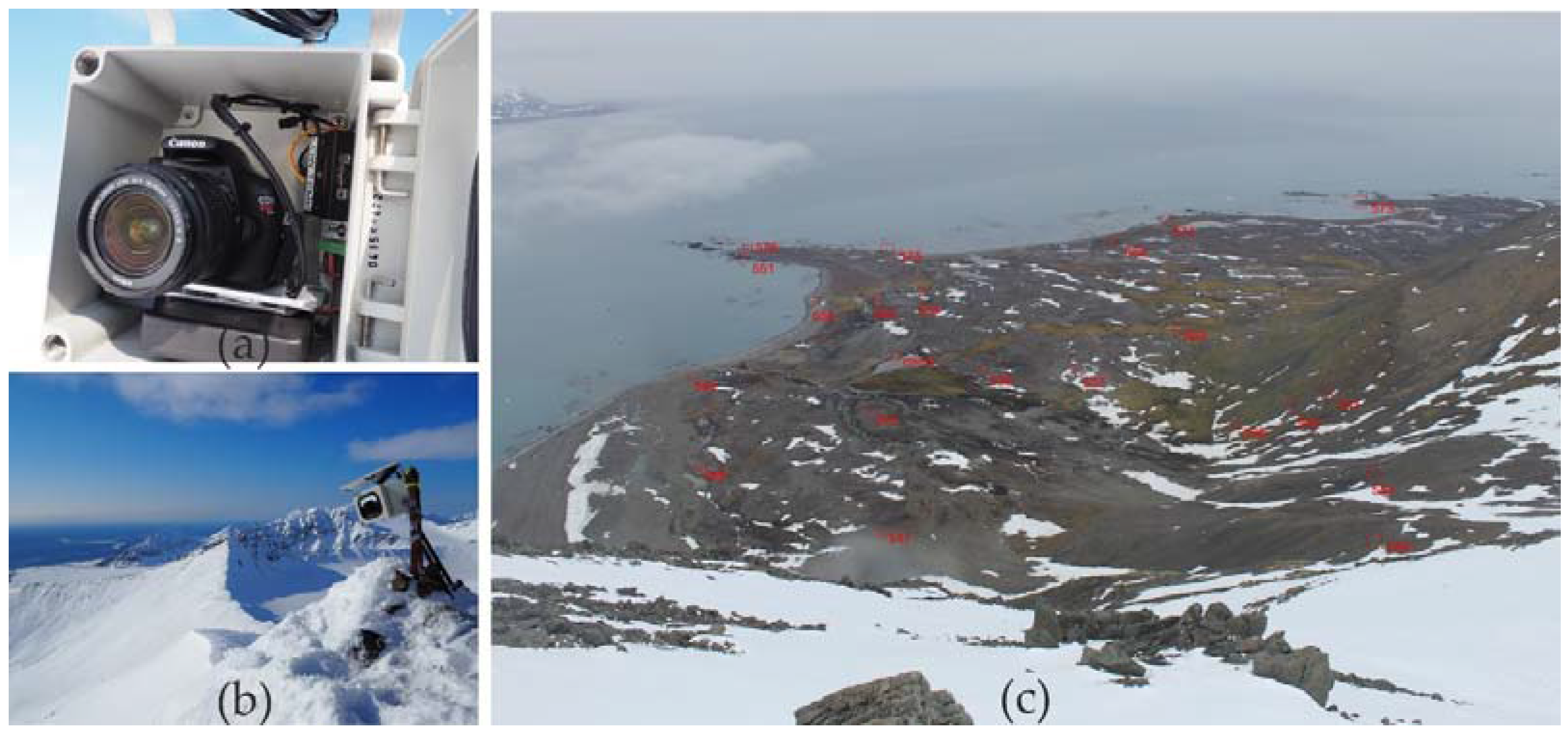
2.3.1. Image Acquisition and Data Preprocessing

An automatic time-lapse camera system (Table 2; Figure 2a) was installed near the summit of Fugleberget (550 m a.s.l., Figure 1a and Figure 2b), overlooking the unglaciated Fuglebekken catchment. In total, the field of view of the camera system amounted to 5.7 km2. However, due to distortion near the image edges, terrain obstacles obscuring part of the terrain (nearly 0.9 km2—see Figure 1a) and difficult referencing in areas far from the camera system, the delineation of the snow extent was limited to an area of 0.72 km2, located in the center of the raw camera images (Figure 2c). The final shape of the classification mask was selected to overlap with the tundra vegetation map ([48]; Figure 1b), which covers the lower Fuglebekken catchment. The original images featured a resolution of 4272 × 2848 pixels (12.2 Mpix) which, after orthorectification (see next sections), resulted in a spatial resolution of the orthoimages of approximately 1 m. As the images were stored with 8-bit color depth, the cell values varied from 0 (black) to 255 (full intensity of the color).
The acquisition of the images started in April 2014. Since then, the system was reinstalled in April in all following years, taking images with a 1-h time step until deinstallation for the winter season. For the purpose of this study, the images were processed until the disappearance of the snow cover in the summer of each season (Table 3).
From the data set of hourly images, a single daily image (if available) was selected. Due to favorable lighting conditions of the scene (least shadows), images acquired between 10 and 11 AM UTC were preferred. If these were not available e.g., due to low-lying clouds, images taken around 11 PM were selected, because the area of interest was in full shade which meant that the scene was evenly illuminated.
Sporadic gaps in the data were caused by low-lying cloud cover or fog obstructing the view towards the area of interest, as well as snow and ice covering the window of the automatic camera system. Furthermore, uneven illumination due to specular reflection of sunlight from water, ice or snow, as well as shadows from mountains and clouds, cause problems in the classification process. These problems were overcome by discarding images unsuitable for further analysis, leaving 203 images which we have used in this study (Table 3).

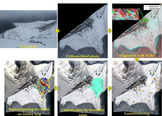
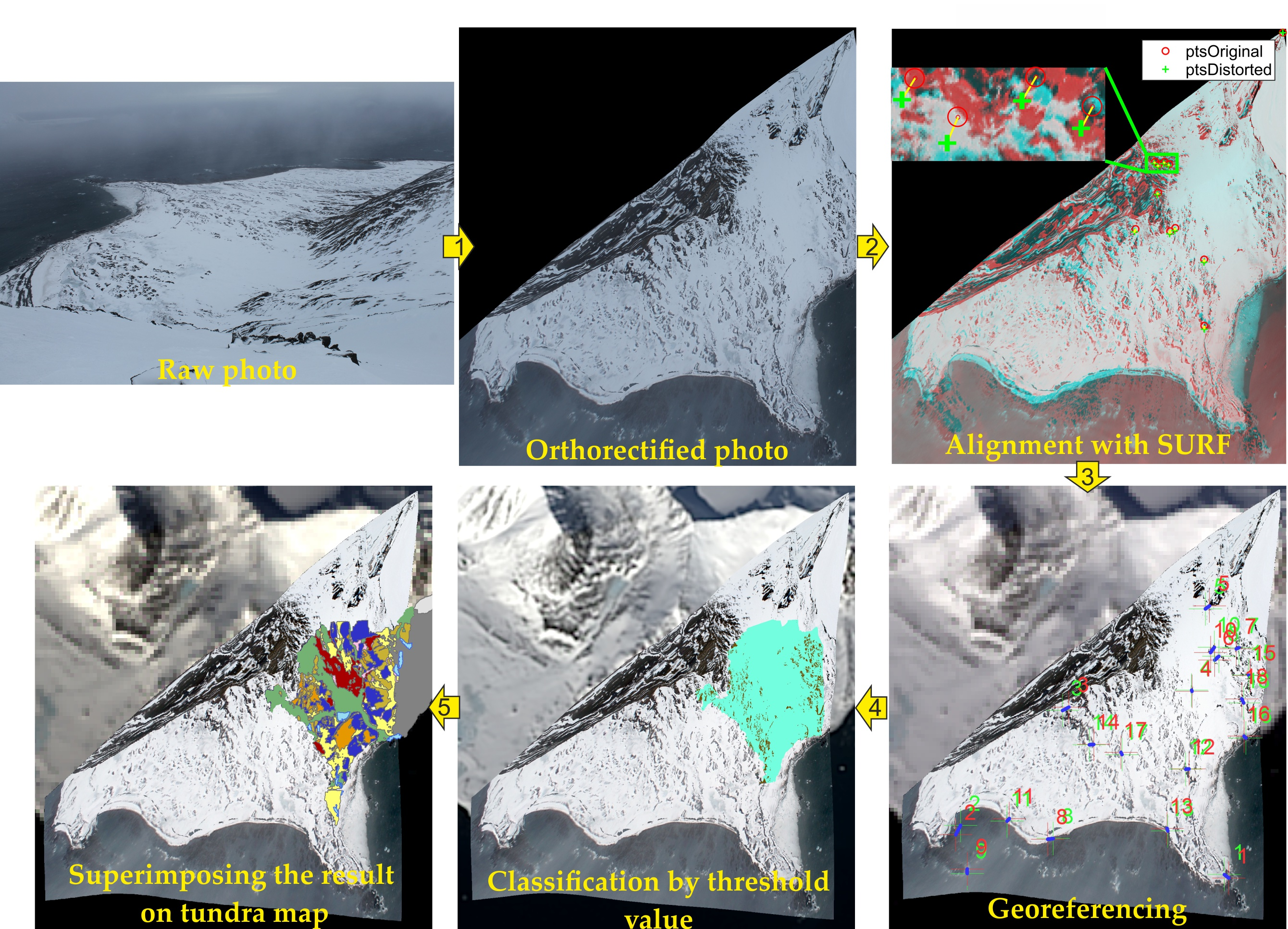
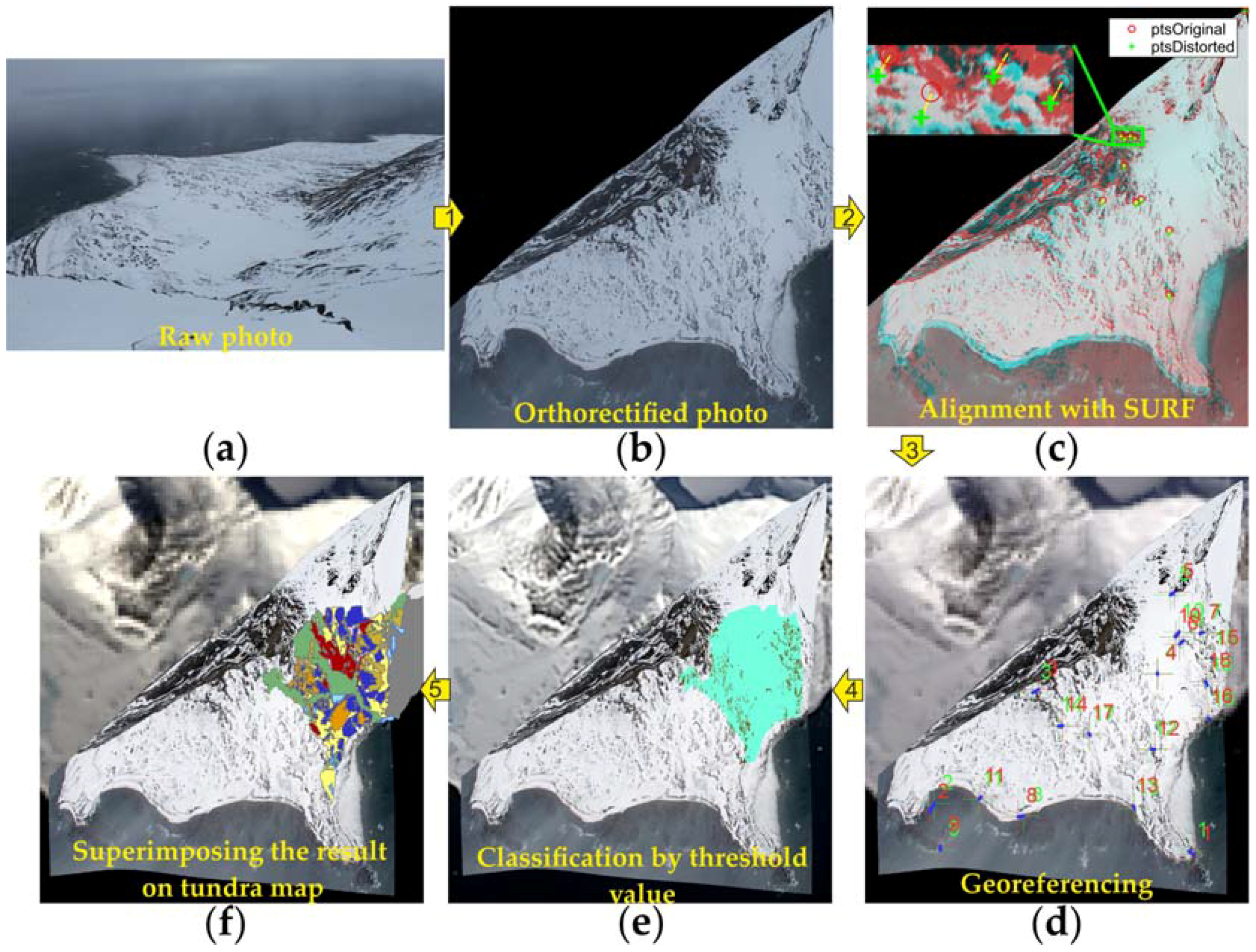
2.3.2. Orthorectification and Georectification

The selected images (Figure 3a) were orthorectified (Figure 3b) in a MATLAB environment using the “Camera Calibration Toolbox” [60] in conjunction with a DEM [57]. Due to strong winds and ground thawing, the camera position and its view angle slightly changed within each season. A continuous workflow with fixed parameters for the camera orientation was therefore not possible, so that the orthorectification was performed independently for subperiods without substantial camera shifts (less than 10 pixels distance between points on two pictures). For this purpose, 17 to 20 characteristic points evenly distributed in the area were used as ground control points (GCPs) (Figure 2c). The average root mean square error (RMSE) of the fit was in the range of 58 to 63 m for the entire camera scene, with a smaller RMSE of 39 m for the study area in the Fuglebekken catchment. After orthorectification, an alignment of the pictures relative to each other was performed, using the MATLAB Computer Vision toolbox and the Speeded-Up Robust Features (SURF) technique [61] (Figure 3c). The employed feature matching algorithm is based on identifying similar patterns found between images. Therefore, the best results were obtained when input images had similar snow coverage.
The orthorectified images were georeferenced in ArcGIS using available GIS materials [48,58] as reference images. For georectification the most rubbersheeting-type “spline” method was used [62], to compensate for the nonlinear distortions produced during orthorectification, and to adjust the orthorectified images as precisely as possible to the base orthophoto map [58] (Figure 3d). As this method exactly transforms the source control points to target control points [63], the obtained RMSE was always close to 0 m. To visualize the general quality of the fit, the RMSE for the standard 1st order polynomial method would be in the range of 13 to 55 m for the whole scene using at minimum 16 referencing points chosen from characteristic terrain features like protruding rocks. The RMSE for only the classification area would reach in worst case 21 m using 46 referencing points. The largest number of reference points (more than 100 in the case of successful image auto registration in ArcGIS) was localized in the Fuglebekken catchment to correctly represent this area.
We emphasize that the SURF alignment and the different georeferencing steps were required to compensate for image shifts due to frequent small camera movements. With a completely stable camera position (which cannot be realistically achieved at the summit of Fugleberget), a simpler workflow would be sufficient.

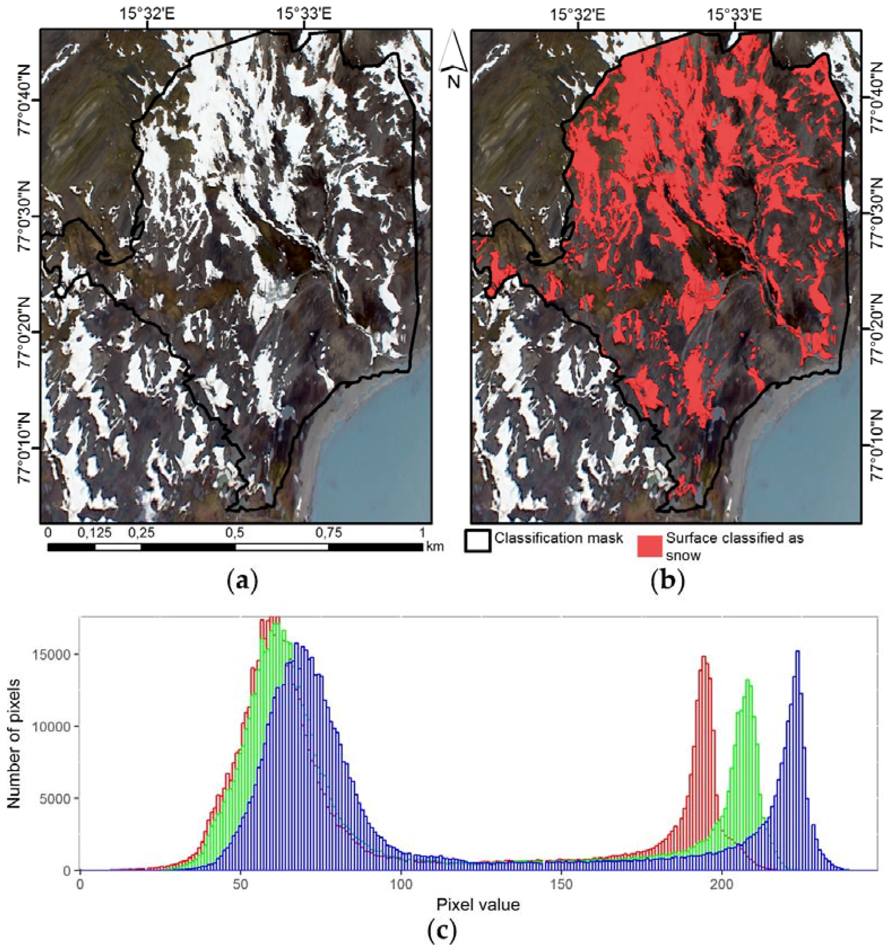
2.3.3. SCE Extraction

To classify the snow cover on the processed time-lapse images, three different approaches were tested: supervised classification, unsupervised classification and threshold filtering. Both unsupervised and supervised classification yielded satisfactory results, but batch processing of a large number of images proved challenging. In the unsupervised classification, a varying number of classes were required to extract snow in different melting stages from the images, since two classes were not always appropriate. On the other hand, a supervised classification required drawing test polygons for every scene with different lighting conditions. However, even this did not always guarantee good results. The most efficient solution was threshold filtering, which could easily be applied simultaneously to multiple scenes. Only the blue band of the images was used, as even the snow in shaded area was characterized by relatively high values in this band. Similar approaches have been successfully used by Salvatori et al. 2011 [64] and Härer et al. 2013 [65]. The threshold values were determined separately for small groups of consecutive pictures with similar lighting conditions. Basing on this assessment, pictures with the same threshold values were grouped in separate geodatabases and processed in ArcGIS (using the developed model available in the supplementary materials). The results of the classification (Figure 3e) were manually evaluated for each picture and, if necessary, images were reclassified using a different threshold value. In general, the threshold value to distinguish snow from snow-free surface was approximately 150 in the blue band, but varied between 115 and 200 (Figure 4) for different illumination and weather conditions. An exception occurred on 23 May 2016, when brownish melt water appeared on the snow surface. In this situation, the threshold value was lowered to 92, which resulted in good classification results. Previous studies using a threshold value in the blue band adopted a threshold value of 127 or more for snow delineation [64,65], which is well in the range of this study. However, 5 of 203 pictures were successfully classified with a lower value, always in situations when brownish meltwater appeared on the snow surface. As this occurred when snow still covered the tundra areas with high reflectance and light colors, lowering the threshold did not produce any misclassifications.
In general, images were classified until the total disappearance of snow from the study area. However, because single pixels in several snow-free scenes were wrongly classified as snow (e.g., a small white cabin, or the Fuglebekken stream reflecting the sun), we defined the complete disappearance date as the first day when SCE decreased below 2% in the study area.

2.3.4. Spatial Analysis

A tundra vegetation map [48] available as a shapefile was superimposed on the classified images in ArcGIS to calculate SCE for different land cover types (Figure 3f). Correlations between SCE and land cover classes were investigated by an analysis of variance (ANOVA) [66] in conjunction with a post-hoc Tukey honest significant difference (HSD) test [67] in R. This statistical procedure was repeated for snow depth and SWE data from manual measurements that were assigned to specific land cover classes.
As classification results from three years were available, it was possible to distinguish local snowbeds. Each pixel was scored from 0 (no snow in all years) to 3 (snow in all years) for “specific melting stages”, i.e., points in time when (nearly) the same SCE was recorded in different years. We defined 72% snow coverage as “early stage”, 33% coverage as “advanced stage” and 4–5% coverage as “late stage”. The SCE thresholds were chosen according to data availability, as these percentages of snow coverage were found in images in all years, which makes them well-suited for comparison.
The dates of snowmelt for points with manually measured snow depths were estimated from the classified images. The date of snow disappearance was defined as the first day when the pixel containing the point and all surroundings cells (nine in total) were classified as snow-free.

3. Results

3.1. Snow Coverage in Fuglebekken Catchment

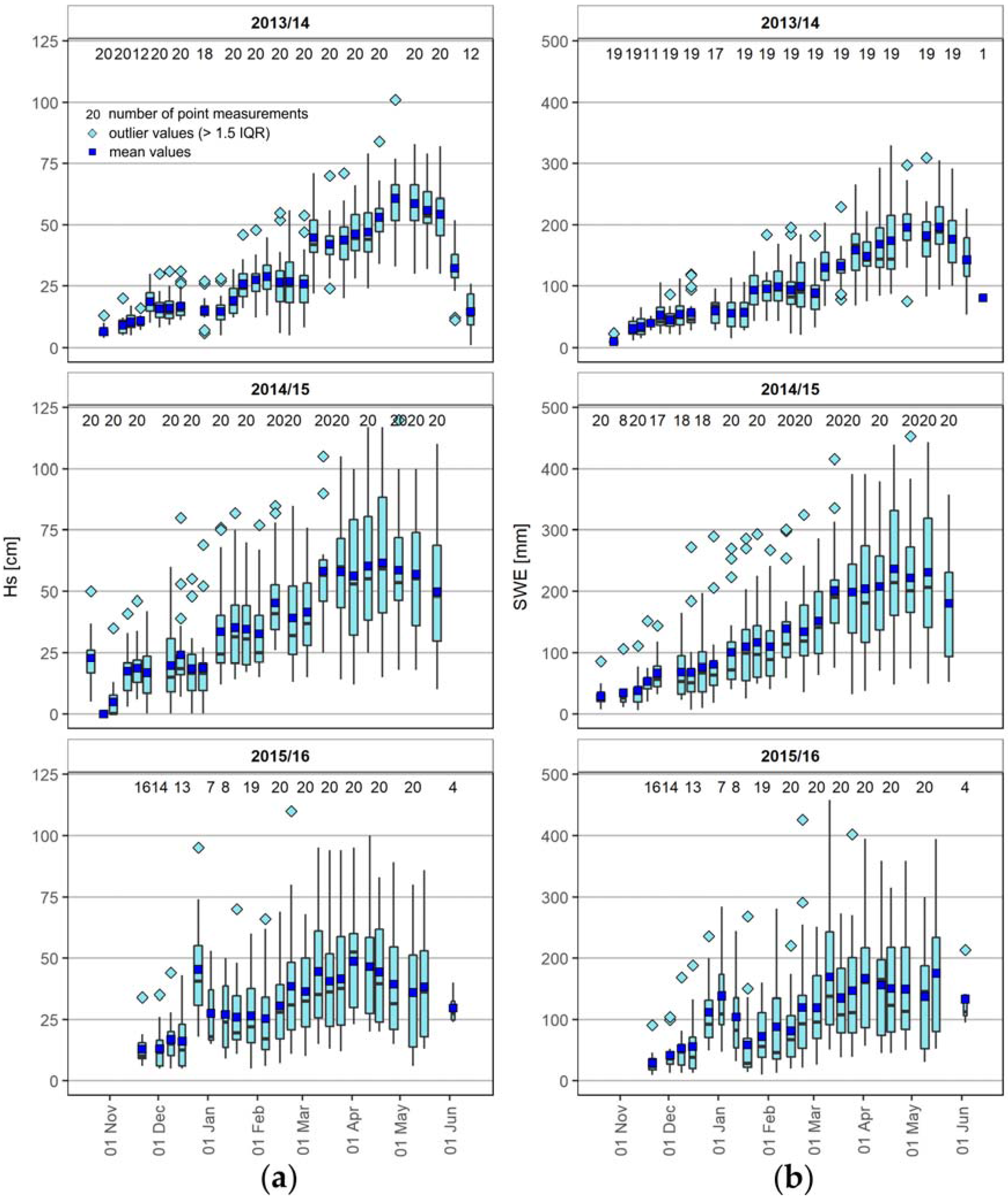
3.1.1. Snow Depth and Water Equivalent

Manual measurements of depths and SWE are available as ground truth information on the distribution of snow in the Fuglebekken catchment (Figure 5). The average values of these measurements were substantially different from snow depths obtained at PPS, with on average 30–40 cm higher values (Figure 5, Table 1). Nevertheless, maximum snow depth occurred at generally the same time in April each year. SWE reached its highest values slightly later, when the snow was saturated with water, probably partly stemming from melt water flowing from the slopes to the lower parts of the catchment. In all years, the highest values of snow depth and SWE were measured at four points in the northern part of the catchment (northernmost points in Figure 1), which correspond to the outlier values in Figure 5. These points are located just under the steep slopes of Fugleberget, where avalanches and slides contribute to snow accumulation. The three years record indicates that the largest outflow of water stored in the tundra snowpack started every time in late May. For example, on 26 May 2014, 177 mm SWE on average was stored in the 54 cm deep snowpack. Within three weeks, the depth of the remaining snow had decreased to 14.5 cm and SWE to approximately 55 mm (measurements from 14 June).

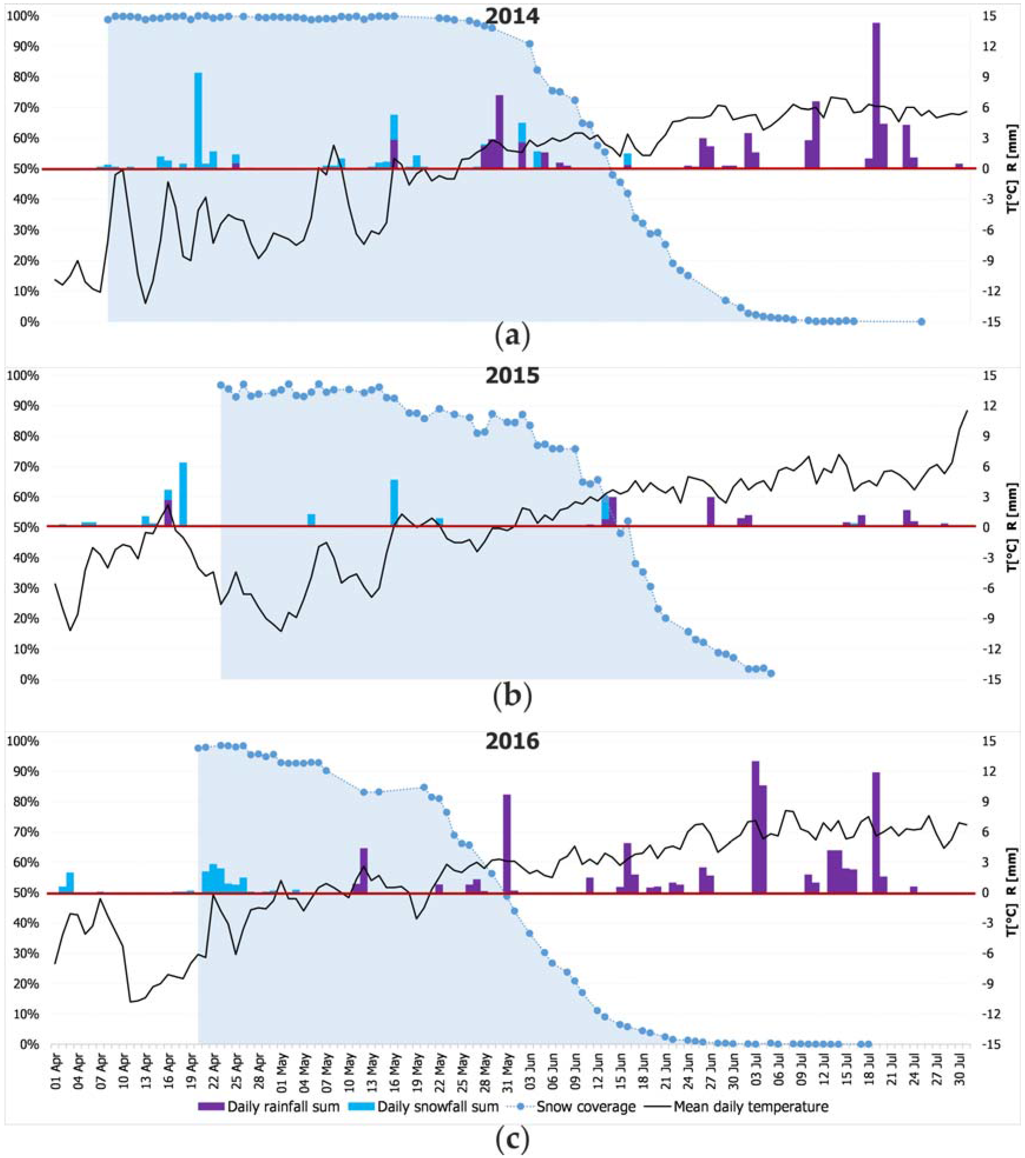
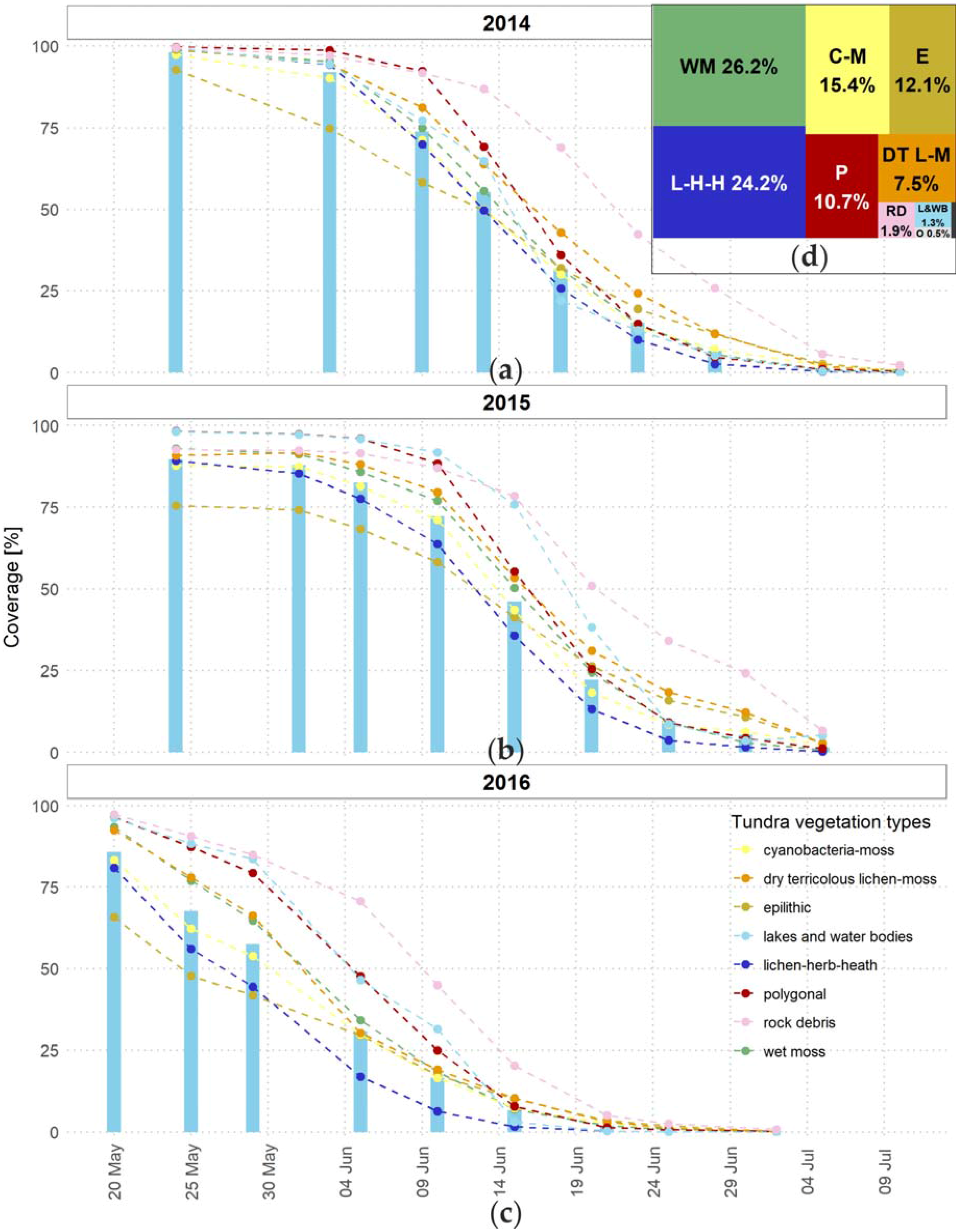
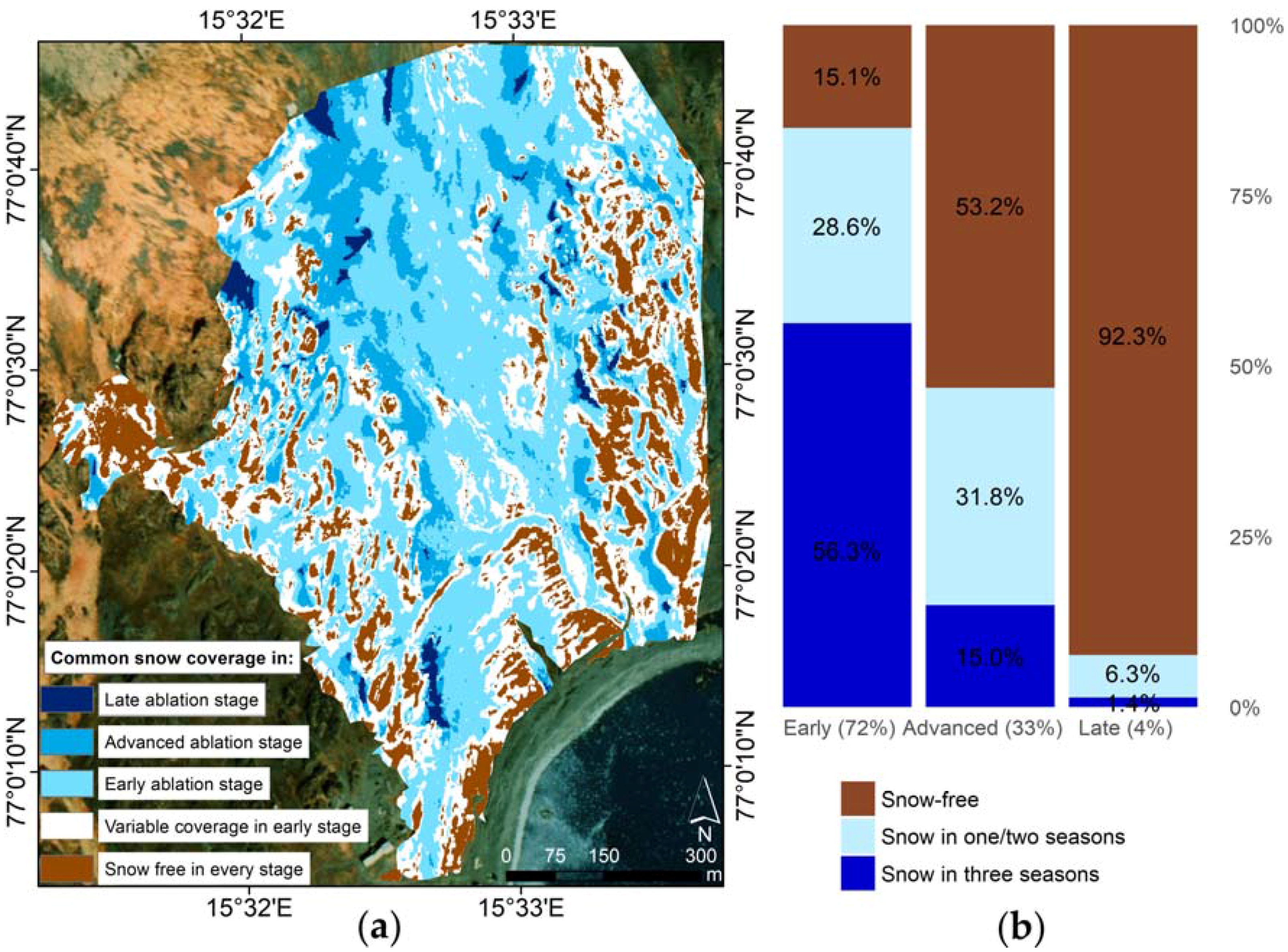
3.1.2. SCE Evolution and Melt-Out Pattern

Figure 6 displays the SCE observations for the melt seasons 2014–2016. Despite some data gaps, SCE was obtained at a high temporal resolution of normally one to three days. Small fluctuations of SCE, were caused by new snowfall, drifting of loose snow or small misclassifications. The SCE curve for 2015 is relatively noisy as a consequence of camera misfocus that reduced the quality of the obtained orthoimages. Nevertheless, the misclassifications were in the range of 3% which was acceptable for all further analyses.
The results indicate that the snow cover in Fuglebekken catchment usually starts to disappear rapidly in late May/early June, when positive air temperatures begin to dominate [43]. The earliest occurrence of bare ground was recorded in 2016, caused by the early onset of above-zero air temperatures in May and generally low snow depths/SWE (Table 1; Figure 5). The longest duration of the snow cover occurred in spring 2015, which was associated with the prevalence of freezing temperatures until the end of May [69] (Table 1). The classified images allow the quantification of SCE losses and determine the exact point in time when SCE drops below 50%, which is considered to be the last day of snow cover in synoptic station records [70,71]. At manned stations, SCE is only visually evaluated by observers, which may lead to data inconsistencies. Automatic stations do not provide such information at all, which is important for climate change monitoring. Results from the time-lapse camera clearly indicate that SCE dropped below 50% on 14 June in 2014, 15 June in 2015 and 30 May in 2016 (Table 4). The snow cover disappeared completely (<2%) from the study area on the following dates: 3 July in 2014, 6 July in 2015 and 22 June in 2016.
The rates of snow disappearance during the study period are presented in Table 4. Although some variability between consecutive years is seen, the total duration of the melt-out period is generally around 3–4 weeks. The first stage of melting was especially variable: snow coverage decreased below 90% relatively early in seasons 2015 and 2016, because areas with shallow snow cover had already melted out during the first melt events. The transition to the next stage (75% SCE) lasted several weeks in 2015 and 2016, mostly due to prolonged cold periods without melt. The main snowmelt period, with the highest rates of SCE decrease (SCE between 75% and 10%) consistently lasted around 3 weeks in all years. In turn, the last melting stage occurred at comparatively lower rates, requiring more than a week for SCE to decrease from 10 to 2% in 2015 and 2016. Small, localized snow patches (SCE < 2%) occurred in the Fuglebekken area until the middle of July.
The multi-year data set facilitates delineation of areas that melt out early, as well as snowbed areas, where snow occurs even in early summer. In general, the melt-out patterns were similar in all years, which is visualized in Figure 7. The “early stage” (72% SCE) occurred on 9 June, 12 June and 24 May in 2014, 2015 and 2016, respectively. The “advanced stage”, (33% SCE) was reached on 17 June 2014, 19 June 2015 and 5 June 2016. The “late stage” (4–5% SCE) was reached on 29 June 2014, 2 July 2015 and 18 June 2016.
A map of the different ablation stages in all years (Figure 7a) shows that snow in each year disappeared first from the rocky terrain located in the eastern and western part of the study area. More snow accumulated in the central part of the study area, which resulted in later melting. The prolonged presence of snow cover in the western part of the catchment (Figure 7a—“advanced” stage) was most likely caused by the prevailing easterly wind direction in the Hornsund area [72], which forms snowdrifts in front of topographic barriers. In the late stage, snow remained only near rocky outcrops and at the foothills of Fugleberget, where the deepest snowpack occurred (Figure 5 outliers). In general, longer occurrence of snow was related to higher snow depths, amounting to 10 to 20 cm larger values during maximum of accumulation on sites where snow remained to the advanced stage, which responded to 50–70 mm higher SWE (Figure 8).
Figure 7 also shows that the melt-out pattern was highly similar in all years (despite changes in the overall timing, Figure 6), with a rather small areal fraction featuring different ablation stages in the different years. Areas with interannual variability of melt-out (snow in one or two years—score 1 or 2), amounted to 28.6% during the early stage, 31.8% in the advanced and 6.3% in the late stage (Figure 7b). By far the largest area was either consistently snow-covered or consistently snow-free in all years for all considered ablation stages. This interannual variability may even be slightly overestimated due to small shifts between superimposed classified pictures, which occurred despite the alignment procedure. Nevertheless, the rates of snowmelt were different despite comparable time of the SCE decrease in the years 2014–2016 (Table 4), because different SWE values were measured during maximum accumulation (Figure 8). It should be noted that some manual measurement points are located in places that show interannual variability in snowmelt, which is visible on Figure 8 (different number of records above the red line on scatterplots). The amount of snow at the same points was variable between the seasons, but in general the points melted out in similar order every year.

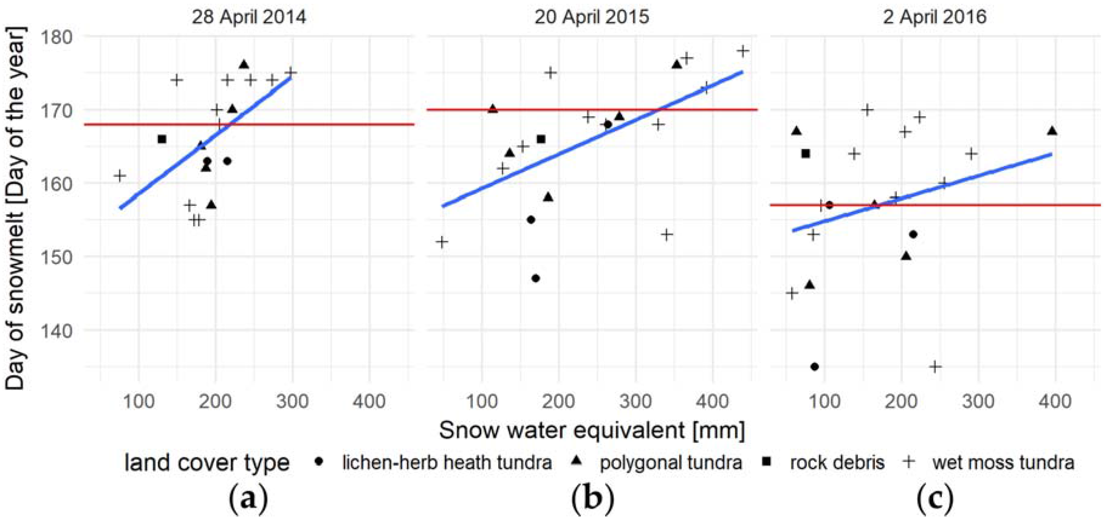
3.2. Relationship between Snow Cover and Vegetation

The SCE data were evaluated against the tundra vegetation map by Migała et al. [48]. The results (Figure 9) show differences in the time of snowmelt for different land cover types. In all years, the lowest SCE in the beginning of the melt-out period was found on epilithic tundra, which is associated with protruding rock formations. During the main melt phase, almost all land cover types were characterized by similar SCE values. The only exception was rock debris without vegetation, which was characterized by high SCE. On this land cover type, snow found in small patches in sheltered places close to rock outcrops melted out last. In contrast, fast snow withdrawal from lichen-herb-heath tundra is distinct in Figure 9. Snowmelt from vegetation types in general shows a consistent interannual pattern, only shifted in time due to different weather conditions (Table 1). In all three years, snow on lichen-herb-heath tundra disappeared entirely when approximately 25% of the rock debris was still snow-covered, resulting in a melt-out time-lag of almost 2 weeks. The largest community in the study area, wet moss tundra, was characterized by only slightly higher SCE values than average, also consistently in all three years.
Statistically significant differences in the ANOVA test were found between SCE, snow depth and SWE measured on various tundra types, although post-hoc analysis with the Tukey HSD test suggest significant differences only between some of the tundra communities. For snow depth, only wet moss tundra featured statistically significant higher average depths in comparison to snow on the other land cover types (Table 5). The significance level was also maintained when 4 outlier points, characterized by the highest snow depths during winter season, were excluded. Wet moss tundra was characterized by the highest average snow depth and SWE compared to other types, with values on average 10 cm (50 mm) higher in the case of the maximum accumulated snow depth (SWE) (see Figure 8). The higher snow depths were in agreement with a higher SCE on wet moss tundra compared to the overall catchment area, which was visible in the earlier stage of snow disappearance (Figure 9). For SCE, only the rock debris type was characterized by statistically significantly greater snow extent during melting (nearly 20 percentage points) in comparison to other land cover types (Figure 9).

4. Discussion

Images obtained from the time-lapse camera system on Fugleberget have been processed to deliver high-quality spatially resolved information on snow cover extent in harsh Arctic conditions. The largest difficulties encountered during this work were small movements of the camera due to strong wind activity and other factors, so that the images needed to be processed with a feature matching algorithm (Figure 3c) in addition to orthorectication and georeferencing. The SURF technique proved to be useful especially in the first phase of the melting when the snow coverage changed very little, or in the summer period, when only snow patches were present on the ground. However, not all camera movements could be compensated by the SURF techniques. Therefore, the final stage of image alignment was completed in ArcGIS. Although the manual alignment of the pictures was accomplished with care, the final classification results are likely to be associated with a certain degree of error, which, however, should be acceptable for most applications. In 2015, camera misfocus led to blurred images, which clearly decreased the precision of the SCE classification (Figure 6b). However, even with these complications, the obtained data constitute a high quality SCE data set, with both spatial and temporal resolution considerably higher than presently achievable with satellite images. The methodology and tools presented in this work, such as the scheme to reduce the effects of camera movements in the spatial analysis, may be applicable to other studies with a similar time-lapse camera setup.
The melt rate obtained in this study is generally compatible with rates in the coastal area near Ny-Ålesund in north-western Svalbard in 2002 [22], where most of the monitored area also melted out within 50 days (see Table 4), with small snow patches that remained one month longer. The reported average melting period was 28 days long, which is generally in line with the 3–4 week-long melt-out period described in our study.
The spatial snow distribution in the study area has been investigated previously, based on a number of point measurements [73,74,75], but the measurement locations were different and focused on capturing the total range of snow depths. Measurements from the spring periods of 1980–1983 indicate an average snow depth of 30 to 60 cm [75], which matches well with results from this study (Figure 5a). Dolnicki [73,74] indicates that in “open” terrain the snow depths generally do not exceed 60 cm, although values above 100 cm are often encountered between rock outcrops. These measurements may correspond to the prolonged snow cover found in this study for the rock debris land cover type (Figure 9).
Previous studies have highlighted the influence of snow cover on vegetation distribution in the Fuglebekken area [48,52]. However, this study is the first to quantify snow ablation and the melt-out patterns in this area. Our analysis suggests weak relationships between the duration of snow cover and the occurrence of specific land cover types. The longest snow cover duration was found on the terrain without plants (“rock debris” type), raising the question of whether the long-lasting snow cover could be one of the reasons for the lack of vegetation. As snow duration is generally strongly related to depth (Figure 8), the rock debris sites should be characterized by the greatest snow thickness. The routine observations of the snow monitoring program near the Polish Polar Station cannot confirm this, because the measurement points were chosen to represent average conditions for hydrology purposes rather than covering different land cover types. This means that no data are available for sites between the rocky outcrops that can accumulate the highest amounts of snow. The earlier disappearance of snow from the dry lichen-herb-heath tundra is likely due to two factors. Firstly, this type of vegetation is linked to Haplic Cryosol, which is the warmest and driest soil type in the studied area [48,49]. Secondly, this vegetation type is confined to dry, flat or only gently sloping sites on raised and exposed marine terraces, where strong wind erosion of snow leads to shallow snow depths. Interestingly, cyanobacteria-moss tundra, which is considered to be a snowbed community in the Fuglebekken area [76], was characterized by relatively average SCE values during the study period (Figure 9), and only some of the snowbed areas (dark blue colors in Figure 7a) coincided with the occurrence of this type of tundra.
In addition to snow cover, soil moisture probably plays a major role in the distribution of vegetation communities in the Fuglebekken catchment [77]. Soil moisture, however, is also closely linked to the spatial variability of snow cover [78], particularly in early summer when snow patches still remain. The highest vegetation indices in the Fuglebekken area were measured for areas covered by wet mosses [79], where large amounts of nitrogen, needed for plant development, were also found [52]. It should be noted that wet mosses were characterized by the largest measured snow depths (Table 5) and slightly increased SCE values compared to other land cover classes (Figure 9). This indicates that the snow cover in some areas might have a positive effect on vegetation communities in the study area.
The Fuglebekken catchment is a focus area for research on various topics, such as permafrost [36,37,73,74], soil nutrients [49,80], hydrology [81], pollutant concentration [42,82] and plant growth [77,83,84]. As all these topics are intimately linked to snow cover, the spatially resolved data sets presented in this study provide valuable background information for ongoing and future research in this region. The automatic camera system on Fugleberget, of which the first data sets are presented in this study, is an important part of long-term snow monitoring in the Hornsund area, which will help answer the question of how the terrestrial cryosphere in the Arctic is responding to rapidly warming climate conditions.

5. Conclusions

In this study, we evaluate the spatial patterns of snowmelt in a high-Arctic tundra environment by using time-lapse imagery obtained from an automatic camera system located on the summit of a mountain. This is the first work that quantifies the spatial distribution of snow in the southern unglaciated part of Svalbard and relates this information to vegetation type occurrence. The methodology proved to be useful for provide data sets on snow cover extent at high spatial and temporal resolution at a small catchment scale with only few data gaps caused by unfavorable weather conditions. Therefore, time-lapse imagery will enhance long-term snow monitoring at PPS in Hornsund, by adding spatial information about snow cover extent, not achievable with traditional measurements.
Based on time-lapse monitoring data supplemented by ground truth information about snow depth and SWE, we show that the melt-out pattern is generally consistent and repetitive between years, despite substantially different weather conditions. The years examined in this study were characterized by different amounts of snow and a different timing of the ablation period, which for example resulted in a two weeks earlier melt-out in 2016. The longest snow durations occurred in the same areas in all seasons (at the foothill of mountain slopes and around rock outcrops), where snow disappeared in late June or early July. In all years the fastest snow withdrawal occurred on protruding rocks connected to epilithic tundra type and wind exposed areas covered mostly by lichen-herb-heath tundra. The main snowmelt period (i.e., the period of SCE decrease from 75% to zero (<2%) snow cover) consistently lasted for about 3 to 4 weeks in the examined years.
The relationship between snow cover and vegetation occurrence was found weaker than assumed. Statistically significant results were found for the “rock debris” type without the vegetation that was characterized by an approximately 20 percentage points larger SCE than other land cover types during the melt season. Furthermore, on wet moss tundra, the snow depth was several centimeters higher in comparison to other plant communities within the snow season. Surprisingly, we found that areas with the longest snow duration did not overlap with the occurrence of snowbed communities (cyanobacteria moss). Therefore, snow depth and the duration of the snow-covered season are not the only decisive factor controlling vegetation distribution in this high-Arctic location.

Supplementary Materials

As part of this article, we provide a model obtained by means of ArcGIS model builder for classification of image stacks in ESRI software. ArcGIS toolbox facilitating the threshold classification and analysis of many images (with parameters set by default to classify 8-bit RGB images into snow/snow-free surfaces) can be found online at: www.mdpi.com/2072-4292/9/7/733/s1. Grouped by years raw, orthorectified and classified images (clipped to the area with the slightest distortions) can be found online at: https://doi.pangaea.de/10.1594/PANGAEA.874387. Data available here are ready to use and provide a quality acceptable for most applications. However, some of the results presented here were done after additional alignment corrections that can be necessary to relate to each other data between consecutive seasons.

Acknowledgments

This work has been (partially) financed from the funds of the Leading National Research Centre (KNOW) received by the Centre for Polar Studies for the period 2014–2018. Daniel Kępski was awarded in VII edition of Anna Pasek Scientific Grant Program and would like to thank foundation for their support in 2015/2016. Time-lapse camera imagery were collected during Snow Monitoring Using Automatic Camera Systems at Svalbard Key Sites project (project No. 236768/E10; Svalbard Science Forum, Research Council of Norway) and Landsat 8 images were available by courtesy of the U.S. Geological Survey. We wish also to thank the Norwegian Polar Institute for sharing their cartographic resources via npolar.no website. This study is partially funded by the Polish National Science Centre through grant No. 2013/09/N/ST10/04105: Impact of climate change on snow cover and hydrological regime of polar non-glaciated catchment, and within statutory activities No. 3841/E-41/S/2017 of the Ministry of Science and Higher Education of Poland. Sebastian Westermann acknowledges financial support by the projects COUP (project No. 244903/E10), SatPerm (project No. 239918) and Permanor (project No. 255331/E10; all Research Council of Norway). We want to sincerely thank reviewers for their useful suggestions that improved structure and clarity of the final text. Heartily thanks for A. Lowell that agreed improving the English language and style.

Author Contributions

The article is a result of collaboration with all listed co-authors. S.W. and B.L. designed the study and processed raw images into orthophotomaps. T.W. provided meteorological and snow depth and density data. B.W. provided spatial data about tundra vegetation and helped with interpretation of them. K.M. contributed to study design and helped with snow extent data analysis. D.K. performed most of data analysis, aligned and classified orhorectified images, produced figures and wrote the majority of the paper. All authors contributed to the final version of the manuscript.

Conflicts of Interest

The authors declare no conflict of interest. The founding sponsors had no role in the design of the study; in the collection, analyses, or interpretation of data; in the writing of the manuscript, and in the decision to publish the results.

References

  1. Evans, B.M.; Walker, D.A.; Benson, C.S.; Nordstrand, E.A.; Petersen, G.W. Spatial interrelationships between terrain, snow distribution and vegetation patterns at an arctic foothills site in Alaska. Ecography 1989, 12, 270–278. [Google Scholar] [CrossRef]
  2. Callaghan, T.V.; Johansson, M.; Brown, R.D.; Groisman, P.Y.; Labba, N.; Radionov, V.; Bradley, R.S.; Blangy, S.; Bulygina, O.N.; Christensen, T.R.; et al. Multiple Effects of Changes in Arctic Snow Cover. AMBIO 2011, 40, 32–45. [Google Scholar] [CrossRef]
  3. Jonas, T.; Rixen, C.; Sturm, M.; Stoeckli, V. How alpine plant growth is linked to snow cover and climate variability. J. Geophys. Res. 2008, 113. [Google Scholar] [CrossRef]
  4. Wahren, C.-H.A.; Walker, M.D.; Bret-Harte, M.S. Vegetation responses in Alaskan arctic tundra after 8 years of a summer warming and winter snow manipulation experiment. Glob. Change Biol. 2005, 11, 537–552. [Google Scholar] [CrossRef]
  5. Wipf, S. Phenology, growth, and fecundity of eight subarctic tundra species in response to snowmelt manipulations. Plant Ecol. 2010, 207, 53–66. [Google Scholar] [CrossRef]
  6. Cooper, E.J.; Dullinger, S.; Semenchuk, P. Late snowmelt delays plant development and results in lower reproductive success in the High Arctic. Plant Sci. 2011, 180, 157–167. [Google Scholar] [CrossRef] [PubMed]
  7. Johansson, M.; Callaghan, T.V.; Bosiö, J.; Åkerman, H.J.; Jackowicz-Korczynski, M.; Christensen, T.R. Rapid responses of permafrost and vegetation to experimentally increased snow cover in sub-arctic Sweden. Environ. Res. Lett. 2013, 8, 035025. [Google Scholar] [CrossRef]
  8. Hülber, K.; Bardy, K.; Dullinger, S. Effects of snowmelt timing and competition on the performance of alpine snowbed plants. Perspect. Plant Ecol. Evol. Syst. 2011, 13, 15–26. [Google Scholar] [CrossRef]
  9. Williams, C.M.; Henry, H.A.L.; Sinclair, B.J. Cold truths: how winter drives responses of terrestrial organisms to climate change: Organismal responses to winter climate change. Biol. Rev. 2015, 90, 214–235. [Google Scholar] [CrossRef] [PubMed]
  10. Wipf, S.; Rixen, C. A review of snow manipulation experiments in Arctic and alpine tundra ecosystems. Polar Res. 2010, 29, 95–109. [Google Scholar] [CrossRef]
  11. Anderson, K.; Gaston, K.J. Lightweight unmanned aerial vehicles will revolutionize spatial ecology. Front. Ecol. Environ. 2013, 11, 138–146. [Google Scholar] [CrossRef]
  12. Gisnås, K.; Westermann, S.; Schuler, T.V.; Litherland, T.; Isaksen, K.; Boike, J.; Etzelmüller, B. A statistical approach to represent small-scale variability of permafrost temperatures due to snow cover. Cryosphere 2014, 8, 2063–2074. [Google Scholar] [CrossRef]
  13. Winther, J.-G.; Godtliebsen, F.; Gerland, S.; Isachsen, P.E. Surface albedo in Ny-Ålesund, Svalbard: variability and trends during 1981–1997. Glob. Planet. Change 2002, 32, 127–139. [Google Scholar] [CrossRef]
  14. Luks, B. Dynamika zmian pokrywy śnieżnej w rejonie południowo-zachodniego Spitsbergenu. Ph.D. Dissertation, Institute of Geophysics, Polish Academy of Sciences, Warszawa, Poland, 2012. [Google Scholar]
  15. Johansen, B.E.; Karlsen, S.R.; Tømmervik, H. Vegetation mapping of Svalbard utilising Landsat TM/ETM+ data. Polar Rec. 2012, 48, 47–63. [Google Scholar] [CrossRef]
  16. Johansen, B.; Tømmervik, H. The relationship between phytomass, NDVI and vegetation communities on Svalbard. Int. J. Appl. Earth Obs. Geoinformation 2014, 27, 20–30. [Google Scholar] [CrossRef]
  17. Karlsen, S.; Elvebakk, A.; Høgda, K.; Grydeland, T. Spatial and Temporal Variability in the Onset of the Growing Season on Svalbard, Arctic Norway — Measured by MODIS-NDVI Satellite Data. Remote Sens. 2014, 6, 8088–8106. [Google Scholar] [CrossRef]
  18. Vickers, H.; Høgda, K.A.; Solbø, S.; Karlsen, S.R.; Tømmervik, H.; Aanes, R.; Hansen, B.B. Changes in greening in the high Arctic: insights from a 30 year AVHRR max NDVI dataset for Svalbard. Environ. Res. Lett. 2016, 11, 105004. [Google Scholar] [CrossRef]
  19. Parajka, J.; Haas, P.; Kirnbauer, R.; Jansa, J.; Blöschl, G. Potential of time-lapse photography of snow for hydrological purposes at the small catchment scale. Hydrol. Process. 2012, 26, 3327–3337. [Google Scholar] [CrossRef]
  20. Garvelmann, J.; Pohl, S.; Weiler, M. From observation to the quantification of snow processes with a time-lapse camera network. Hydrol. Earth Syst. Sci. 2013, 17, 1415–1429. [Google Scholar] [CrossRef]
  21. Smith, K.L.; Baldwin, R.J.; Glatts, R.C.; Chereskin, T.K.; Ruhl, H.; Lagun, V. Weather, ice, and snow conditions at Deception Island, Antarctica: long time-series photographic monitoring. Deep Sea Res. Part II Top. Stud. Oceanogr. 2003, 50, 1649–1664. [Google Scholar] [CrossRef]
  22. Hinkler, J.; Ørbæk, J.B.; Hansen, B.U. Detection of spatial, temporal, and spectral surface changes in the Ny-Ålesund area 79° N, Svalbard, using a low cost multispectral camera in combination with spectroradiometer measurements. Phys. Chem. Earth Parts ABC 2003, 28, 1229–1239. [Google Scholar] [CrossRef]
  23. Buus-Hinkler, J.; Hansen, B.U.; Tamstorf, M.P.; Pedersen, S.B. Snow-vegetation relations in a High Arctic ecosystem: Inter-annual variability inferred from new monitoring and modeling concepts. Remote Sens. Environ. 2006, 105, 237–247. [Google Scholar] [CrossRef]
  24. Laffly, D.; Bernard, E.; Griselin, M.; Tolle, F.; Friedt, J.-M.; Martin, G.; Marlin, C. High temporal resolution monitoring of snow cover using oblique view ground-based pictures. Polar Rec. 2012, 48, 11–16. [Google Scholar] [CrossRef]
  25. Bernard, É.; Friedt, J.-M.; Tolle, F.; Griselin, M.; Martin, G.; Laffly, D.; Marlin, C. Monitoring seasonal snow dynamics using ground based high resolution photography (Austre Lovenbreen, Svalbard, 79 N). ISPRS J. Photogramm. Remote Sens. 2013, 75, 92–100. [Google Scholar] [CrossRef]
  26. Hagen, D.; Vistad, O.; Eide, N.E.; Flyen, A.; Fangel, K. Managing visitor sites in Svalbard: from a precautionary approach towards knowledge-based management. Polar Res. 2012, 31, 18432. [Google Scholar] [CrossRef]
  27. Chang, M.; Bonnet, P. Monitoring in a High-Arctic Environment: Some Lessons from MANA. IEEE Pervasive Comput. 2010, 9, 16–23. [Google Scholar] [CrossRef]
  28. Vogel, S.W. Usage of high-resolution Landsat 7 band 8 for single-band snow-cover classification. Ann. Glaciol. 2002, 34, 53–57. [Google Scholar] [CrossRef]
  29. Cortés, G.; Girotto, M.; Margulis, S.A. Analysis of sub-pixel snow and ice extent over the extratropical Andes using spectral unmixing of historical Landsat imagery. Remote Sens. Environ. 2014, 141, 64–78. [Google Scholar] [CrossRef]
  30. Vikhamar, D.; Solberg, R. Snow-cover mapping in forests by constrained linear spectral unmixing of MODIS data. Remote Sens. Environ. 2003, 88, 309–323. [Google Scholar] [CrossRef]
  31. Grenfell, T.C.; Perovich, D.K. Seasonal and spatial evolution of albedo in a snow-ice-land-ocean environment. J. Geophys. Res. 2004, 109. [Google Scholar] [CrossRef]
  32. Lynch, A.H.; McGinnis, D.L.; Bailey, D.A. Snow-albedo feedback and the spring transition in a regional climate system model: Influence of land surface model. J. Geophys. Res. Atmospheres 1998, 103, 29037–29049. [Google Scholar] [CrossRef]
  33. Chapin, F.S.; Sturm, M.; Serreze, M.C.; McFadden, J.P.; Key, J.R.; Lloyd, A.H.; McGuire, A.D.; Rupp, T.S.; Lynch, A.H.; Schimel, J.P.; et al. Role of land-surface changes in Arctic summer warming. Science 2005, 310, 657–660. [Google Scholar] [CrossRef]
  34. Westermann, S.; Lüers, J.; Langer, M.; Piel, K.; Boike, J. The annual surface energy budget of a high-arctic permafrost site on Svalbard, Norway. The Cryosphere 2009, 3, 245–263. [Google Scholar] [CrossRef]
  35. Zhang, T. Influence of the seasonal snow cover on the ground thermal regime: An overview. Rev. Geophys. 2005, 43. [Google Scholar] [CrossRef]
  36. Dolnicki, P.; Grabiec, M.; Puczko, D.; Gawor, Ł.; Budzik, T.; Klementowski, J. Variability of temperature and thickness of permafrost active layer at coastal sites of Svalbard. Pol. Polar Res. 2013, 34, 353–374. [Google Scholar] [CrossRef]
  37. Wawrzyniak, T.; Osuch, M.; Napiórkowski, J.; Westermann, S. Modelling of the thermal regime of permafrost during 1990–2014 in Hornsund, Svalbard. Pol. Polar Res. 2016, 37, 219–242. [Google Scholar] [CrossRef]
  38. Roesch, A. Evaluation of surface albedo and snow cover in AR4 coupled climate models. J. Geophys. Res. 2006, 111. [Google Scholar] [CrossRef]
  39. Rechid, D.; Hagemann, S.; Jacob, D. Sensitivity of climate models to seasonal variability of snow-free land surface albedo. Theor. Appl. Climatol. 2009, 95, 197–221. [Google Scholar] [CrossRef]
  40. Pimentel, R.; Herrero, J.; Polo, M.J. Subgrid parameterization of snow distribution at a Mediterranean site using terrestrial photography. Hydrol. Earth Syst. Sci. 2017, 21, 805–820. [Google Scholar] [CrossRef]
  41. Karczewski, A.; Kostrzewski, A.; Marks, L. Raised marine terraces in the Hornsund area (northern part), Spitsbergen. Pol. Polar Res. 1981, 1, 39–50. [Google Scholar]
  42. Wojtuń, B.; Samecka-Cymerman, A.; Kolon, K.; Kempers, A.J.; Skrzypek, G. Metals in some dominant vascular plants, mosses, lichens, algae, and the biological soil crust in various types of terrestrial tundra, SW Spitsbergen, Norway. Polar Biol. 2013, 36, 1799–1809. [Google Scholar] [CrossRef]
  43. Marsz, A.A.; Styszyńska, A. Climate and climate change at Hornsund, Svalbard; Gdynia Maritime University: Gdynia, Poland, 2013. [Google Scholar]
  44. Łupikasza, E. Zmienność występowania opadów deszczu i śniegu w Hornsundzie w okresie lipiec 1978-grudzień 2002. Probl. Klimatol. Polarnej 2003, 13, 93–105. [Google Scholar]
  45. Miętus, M. Snow depth at the Hornsund Station, Spitsbergen in 1978-1986. Pol. Polar Res. 1991, 12, 223–228. [Google Scholar]
  46. Førland, E.J.; Benestad, R.; Hanssen-Bauer, I.; Haugen, J.E.; Skaugen, T.E. Temperature and Precipitation Development at Svalbard 1900–2100. Adv. Meteorol. 2011, 2011, 1–14. [Google Scholar] [CrossRef]
  47. Caputa, Z.; Leszkiewicz, J. Klasyfikacja zim w polskiej stacji polarnej w Hornsundzie (SW Spitsbergen) w okresie 1978/1979-2014/2015. Probl. Klimatol. Polarnej 2015, 25, 169–178. [Google Scholar]
  48. Migała, K.; Wojtuń, B.; Szymański, W.; Muskała, P. Soil moisture and temperature variation under different types of tundra vegetation during the growing season: A case study from the Fuglebekken catchment, SW Spitsbergen. CATENA 2014, 116, 10–18. [Google Scholar] [CrossRef]
  49. Szymański, W.; Wojtuń, B.; Stolarczyk, M.; Siwek, J.; Waścińska, J. Organic carbon and nutrients (N, P) in surface soil horizons in a non-glaciated catchment, SW Spitsbergen. Pol. Polar Res. 2016, 37, 49–66. [Google Scholar]
  50. Elvebakk, A. A survey of plant associations and alliances from Svalbard. J. Veg. Sci. 1994, 5, 791–802. [Google Scholar] [CrossRef]
  51. Walker, D.A.; Billings, W.D.; De Molenaar, J.G. Snow-vegetation interactions in tundra environments. In Snow Ecology: An Interdisciplinary Examination of Snow-Covered Ecosystems; Jones, H.G., Pomeroy, J.W., Walker, D.A., Hoham, R.W., Eds.; Cambridge University Press: New York, NY, USA, 2001; pp. 266–324. [Google Scholar]
  52. Skrzypek, G.; Wojtuń, B.; Richter, D.; Jakubas, D.; Wojczulanis-Jakubas, K.; Samecka-Cymerman, A. Diversification of Nitrogen Sources in Various Tundra Vegetation Types in the High Arctic. PLoS ONE 2015, 10. [Google Scholar] [CrossRef]
  53. Borysiak, J.; Ratyńska, H. Stan badań nad szatą roślinną Spitsbergenu ze szczególnym uwzględnieniem rejonów Bellsundu, Hornsundu i Kaffiøyry. In Warsztaty Glacjologiczne SPITSBERGEN 2004. Glacjologia, Geomorfologia I Sedymentologia środowiska Polarnego Spitsbergenu; Stowarzyszenie Geomorfologów Polskich: Poznań, Poland, 2004; pp. 248–260. [Google Scholar]
  54. Isaksen, K. The breeding population of little auk (Alle alle) in colonies in Hornsund and northwestern Spitsbergen. In Seabird population in the northern Barents Sea; Isaksen, K., Bakken, V., Eds.; Norsk Polarinstitutt: Oslo, Norway, 1995; pp. 49–57. [Google Scholar]
  55. Kwasniewski, S.; Gluchowska, M.; Jakubas, D.; Wojczulanis-Jakubas, K.; Walkusz, W.; Karnovsky, N.; Blachowiak-Samolyk, K.; Cisek, M.; Stempniewicz, L. The impact of different hydrographic conditions and zooplankton communities on provisioning Little Auks along the West coast of Spitsbergen. Prog. Oceanogr. 2010, 87, 72–82. [Google Scholar] [CrossRef]
  56. Guide to Meteorological Instruments and Methods of Observation WMO-No. 8. Available online: https://www.wmo.int/pages/prog/gcos/documents/gruanmanuals/CIMO/CIMO_Guide-7th_Edition-2008.pdf (accessed on 14 July 2017).
  57. Norwegian Polar Institute Terrengmodell Svalbard (S0 Terrengmodell); Norwegian Polar Institute: 2014. Available online: https://doi.org/10.21334/npolar.2014.dce53a47 (accessed on 9 April 2017).
  58. Kolondra, L. Polish Polar Station and Surrounding Areas, Spitsbergen. Orthophotomap 1: 5 000; Katowice Government: Katowice, Poland, 2003.
  59. Time-Lapse Camera Package|Products|Harbortronics. Available online: https://www.harbortronics.com/Products/TimeLapsePackage/ (accessed on 14 July 2017).
  60. Camera Calibration Toolbox for Matlab. Available online: http://www.vision.caltech.edu/bouguetj/calib_doc/ (accessed on 29 May 2017).
  61. Bay, H.; Ess, A.; Tuytelaars, T.; Van Gool, L. Speeded-up robust features (SURF). Comput. Vis. Image Underst. 2008, 110, 346–359. [Google Scholar] [CrossRef]
  62. Affek, A. Georeferencing of historical maps using GIS, as exemplified by the Austrian Military Surveys of Galicia. Geogr. Pol. 2013, 86, 375–390. [Google Scholar] [CrossRef]
  63. Fundamentals of georeferencing a raster dataset—Help|ArcGIS Desktop. Available online: http://desktop.arcgis.com/en/arcmap/latest/manage-data/raster-and-images/fundamentals-for-georeferencing-a-raster-dataset.htm (accessed on 9 April 2017).
  64. Salvatori, R.; Plini, P.; Giusto, M.; Valt, M.; Salzano, R.; Montagnoli, M.; Cagnati, A.; Crepaz, G.; Sigismondi, D. Snow cover monitoring with images from digital camera systems. Ital. J. Remote Sens. 2011, 137–145. [Google Scholar] [CrossRef]
  65. Härer, S.; Bernhardt, M.; Corripio, J.G.; Schulz, K. Practise–photo rectification and classification software (v. 1.0). Geosci. Model Dev. 2013, 6, 837–848. [Google Scholar] [CrossRef]
  66. Kabacoff, R. Analysis of variance. In R in Action: Data Analysis and Graphics with R; Stirling, S., Welch, L., Eds.; Manning Publications Co.: Shelter Island, USA, 2015. [Google Scholar]
  67. Abdi, H.; Williams, L.J. Tukey’s honestly significant difference (HSD) test. Encycl. Res. Des. 2010, 1, 1–5. [Google Scholar]
  68. Williamson, D.F.; Parker, R.A.; Kendrick, J.S. The box plot: a simple visual method to interpret data. Ann. Intern. Med. 1989, 110, 916–921. [Google Scholar] [CrossRef] [PubMed]
  69. Łaszyca, E.; Perchaluk, J.; Wawrzyniak, T. Meteorological Bulletin. Spitsbergen - Hornsund. May 2015. Available online: http://hornsund.igf.edu.pl/Biuletyny/BIULETYN_37/report_2015_05.pdf (accessed on 14 July 2017).
  70. Janiszewski, F. Instrukcja dla stacji meteorologicznych; Wydawnictwa Komunikacji i Lączności: Warszawa, Poland, 1962; ISBN 978-83-220-0329-9. [Google Scholar]
  71. Snow Measurement Guidelines for National Weather Service Surface Observing Programs. Available online: http://www.nws.noaa.gov/os/coop/reference/Snow_Measurement_Guidelines.pdf (accessed on 14 July 2017).
  72. Ferdynus, J.; Styszyńska, A. Temperatura powietrza a kierunek wiatru w Hornsundzie (1978-2009). Probl. Klimatol. Polarnej 2011, 21, 197–211. [Google Scholar]
  73. Dolnicki, P. Wplyw pokrywy śnieżnej na termikę i grubość warstwy czynnej zmarzliny w obszarze tundrowym rejonu Polskiej Stacji Polarnej (SW Spitsbergen). Probl. Klimatol. Polarnej 2002, 12, 107–116. [Google Scholar]
  74. Dolnicki, P. Zmienna grubość pokrywy śnieżnej na tundrze jako przyczyna zróżnicowania przestrzennego grubości warstwy czynnej na przykładzie wschodniej Fuglebergsletty (SW Spitsbergen). Probl. Klimatol. Polarnej 2015, 25, 191–200. [Google Scholar]
  75. Migała, K.; Pereyma, J.; Sobik, M. Akumulacja śnieżna na południowym Spitsbergenie. In Wyprawy Polarne Uniwersytetu Ślaskiego 1980-1984; Bajerowa, I., Ed.; Uniwersytet Śląski: Katowice, Poland, 1988; pp. 48–63. [Google Scholar]
  76. Węgrzyn, M.; Wietrzyk, P. Phytosociology of snowbed and exposed ridge vegetation of Svalbard. Polar Biol. 2015, 38, 1905–1917. [Google Scholar] [CrossRef]
  77. Opała-Owczarek, M.; Pirożnikow, E.; Owczarek, P.; Szymański, W.; Luks, B.; Kępski, D.; Szymanowski, M.; Wojtuń, B.; Migała, K. The influence of abiotic factors on the growth of two vascular plant species (Saxifraga oppositifolia and Salix polaris) in the High Arctic. CATENA under review.
  78. Williams, C.J.; McNamara, J.P.; Chandler, D.G. Controls on the temporal and spatial variability of soil moisture in a mountainous landscape: the signature of snow and complex terrain. Hydrol. Earth Syst. Sci. 2009, 13, 1325–1336. [Google Scholar] [CrossRef]
  79. Hobbler, A. Thermal characteristics of tundra, based on satellite data (Fuglebekken Basin, SW Spitsbergen). Master’s Thesis, University of Wroclaw, Wrocław, Poland, 2011. [Google Scholar]
  80. Szymański, W.; Skiba, S.; Wojtuń, B. Distribution, genesis, and properties of Arctic soils: a case study from the Fuglebekken catchment, Spitsbergen. Pol. Polar Res. 2013, 34, 289–304. [Google Scholar] [CrossRef]
  81. Wawrzyniak, T.; Osuch, M.; Nawrot, A.; Napiorkowski, J.J. Run-off modelling in an Arctic unglaciated catchment (Fuglebekken, Spitsbergen). Ann. Glaciol. 2017, 1–11. [Google Scholar] [CrossRef]
  82. Polkowska, Ż.; Cichała-Kamrowska, K.; Ruman, M.; Kozioł, K.; Krawczyk, W.E.; Namieśnik, J. Organic Pollution in Surface Waters from the Fuglebekken Basin in Svalbard, Norwegian Arctic. Sensors 2011, 11, 8910–8929. [Google Scholar] [CrossRef] [PubMed]
  83. Opaliński, K.W. Primary production and organic matter destruction in Spitsbergen tundra. Pol. Polar Res. 1991, 12, 419–434. [Google Scholar]
  84. Owczarek, P.; Opała, M. Dendrochronology and extreme pointer years in the tree-ring record (AD 1951–2011) of polar willow from southwestern Spitsbergen (Svalbard, Norway). Geochronometria 2016, 43, 84–95. [Google Scholar] [CrossRef]
Figure 1. Location of the study area. (a) Overview with denoted extent of the camera view and the polygon used as the classification mask. (b) Zoom to the classification area with superimposed vegetation map. The detailed characteristics of specific plant communities are described in Wojtuń et al. 2013 [42].
Remotesensing 09 00733 g001
Figure 2. Time-lapse camera set: (a) Internal view; (b) Placement near the Fugleberget summit; (c) View from the camera (16 June 2016) with marked location of all the Ground Control Points (GCP) used in the orthorectification process.
Remotesensing 09 00733 g002
Figure 3. Workflow for the images obtained from the time-lapse camera on the example of picture from 4 May 2016: (a) raw photo from the camera; (b) picture after the orthorectification process; (c) picture superimposed on reference scene. Marked characteristic terrain features recognized on both pictures by SURF algorithm (“ptsOriginal”—features on the reference scene; “ptsDistorted”—the same features identified on the input image (4 May 2016)) and used in alignment process compensating the camera movements; (d) picture embedded in geographical space (Landsat 8 scene from 28 April 2016 in the background) with marked GCPs used in georeferencing process; (e) Results of pixel classification into snow/snow-free surfaces using threshold value in blue band, clipped to the study area; (f) processed picture with superimposed the land cover map used in spatial analysis.
Remotesensing 09 00733 g003
Figure 4. Classification example for 5 June 2016. (a) Orthoimage zoomed to classification area; (b) Classification result with threshold value in blue band set to 140; (c) Frequency histogram of RGB values with characteristic bimodal distribution—note that the distance between modal values is largest for the blue band.
Remotesensing 09 00733 g004
Figure 5. Results of weekly (a) snow depth and (b) snow water equivalent manual measurements in the Fuglebekken catchment in 2013/14, 2014/15 and 2015/16 in boxplot format [68].
Remotesensing 09 00733 g005
Figure 6. Evolution of SCE in Fuglebekken catchment obtained from the time-lapse camera images in spring (a) 2014, (b) 2015 and (c) 2016; each blue point represents a classified image, daily meteorological data are shown in the background.
Remotesensing 09 00733 g006
Figure 7. Snow cover distribution in the Fuglebekken catchment based on the 2014–2016 data set in specific melting stages: early (~72% snow coverage), advanced (~33%) and late (~4%). (a) Results of SCE superimposition for three years. (b) Surface percentage of snow coverage during the three stages.
Remotesensing 09 00733 g007
Figure 8. Relationship between date of snowmelt on manual soundings sites and SWE measured there during the maximum accumulation time that occurred: (a) 28 April in 2014, (b) 20 April in 2015 and (c) 2 April in 2016. Red horizontal line indicate the date of advanced stage occurrence (~33% SCE), blue line is a linear regression.
Remotesensing 09 00733 g008
Figure 9. Evolution of snow coverage on various types of land cover in Fuglebekken catchment at approximately 5 day intervals in spring: (a) 2014, (b) 2015 and (c) 2016. Blue bars represent SCE in the whole study area. (d) The share of individual land cover types in the study area. Two tundra vegetation types covering the lowest percentage of study area were omitted in spatial analysis: ornitocoprophilus (O) tundra (0.5%) and geophytic initial (GI) tundra (0.2%).
Remotesensing 09 00733 g009
Table 1. Meteorological data from PPS in the snow seasons 2013/14, 2014/15 and 2015/2016. Extreme values are highlighted. Percentage of snowfall (snow pellets included) in the total precipitation sum calculated from event duration.
Month2013/142014/152015/161978–2016 2
Mean T 1 (°C)Total R 1 (mm)% of SnowfallMean Hs 1 (cm)Mean T (°C)Total R (mm)% of SnowfallMean Hs (cm)Mean T (°C)Total R (mm)% of SnowfallMean Hs (cm)Mean T (°C)Total R (mm)% of SnowfallMean Hs (cm)
October−2.734825−0.365666−0.293561−2.852663
November−6.127897−4.438715−2.439734−640797
December−6.0258110−7.691008−4.6457513−8.9338811
January−3.0327512−5.919899−2.4457410−9.9348817
February−0.989320−11.3498815−3.91610011−10289122
March−6.8549134−5.3409323−5.5448013−10.2309026
April−7.3179637−4.2139717−5.0410021−8.1228929
May−1.9237238−2.8899101.030719−2.6228125
June3.3171642.991223.8172-2.127237
October–June−3.52367818−4.32498211−2.13327210−7.22607915
1 T—air temperature; R—precipitation sum; Hs—snow depth. 2 snow depth data are collected in PPS since winter 1983/1984, temperature and precipitation since 1978.
Table 2. Characteristics and settings of used time-lapse set.
EquipmentApertureFocusISO SensitivityShutter SpeedCapture FrequencyFocal Length
Canon EOS REBEL T3 (1200D) camera with Harbortronics DigiSnap 2000 intervalometer powered by 11.1 V 9000 mAh lithium polymer battery and 5 Watt solar panel 1f/8manual100Auto-mode1 h18–23 mm 2
1 older version of Harbortronics Time Lapse Package [59].2 21 mm in 2014, 23 mm in 2015, 18 mm in 2016.
Table 3. Information on the data collection in Fuglebekken catchment.
YearDate of Initial DeploymentDate of Last Processed PictureNumber of Processed PicturesDays between Dates (Demanded Amount of Pictures)Date of Deinstallation
20148 April25 July8110817 October
201523 April5 July60735 November 1
201620 April18 July628929 July
1 already on polar night (occurring from 1 November to 12 February).
Table 4. Time needed to fully melt the snow cover starting from different SCE values in the period 2014–2016. Dates for specific SCE were interpolated in case of missing data.
Snow CoverageOccurrence Time in 2014Days to MeltOccurrence Time in 2015Days to MeltOccurrence Time in 2016Days to Melt
90%3 June3017 May508 May45
75%5 June2810 June2624 May29
50%14 June1915 June2130 May23
25%21 June1220 June167 June15
10%27 June627 June913 June9
Total disappearance 13 July06 July022 June0
1 understood as in the text—the first day with snow coverage below 2% in the study area.
Table 5. Statistically significant (p value < 0.05) mutual relations between snow depth on different land cover types. The analysis was performed for the whole period 2014–2016 with date as covariate (after excluding outlier values at the foothill of Fugleberget Mountain).
Type 1Type 2Mean Difference (cm)Lower End Point of Confidence Interval (cm)Upper End Point of Confidence Interval (cm)p Value
wet moss tundraRock debris+7.9+3.4+12.40.0000219
wet moss tundrapolygonal tundra+4.2+1.6+6.70.0000833
wet moss tundracyanobacteria-moss tundra+6.2+1.7+10.60.0014096
wet moss tundralichen-herb-heath tundra+4.2+0.6+7.80.0136878

