Bathymetry of the Coral Reefs of Weizhou Island Based on Multispectral Satellite Images
by
Rongyong Huang
1,2,3, 
Kefu Yu
1,2,3,*,
Yinghui Wang
1,2,3,
Jikun Wang
1,2,3,
Lin Mu
4 and
Wenhuan Wang
1,2,3 1
Coral Reef Research Centre of China, Guangxi University, Nanning 530004, China
2
Guangxi Laboratory on the Study of Coral Reefs in the South China Sea, Guangxi University, Nanning 530004, China
3
School of Marine Sciences, Guangxi University, Nanning 530004, China
4
Institute of Complexity Science and Big Data Technology, Guangxi University, Nanning 530004, China
*
Author to whom correspondence should be addressed.
Remote Sens. 2017, 9(7), 750; https://doi.org/10.3390/rs9070750
Submission received: 26 May 2017
/
Revised: 13 July 2017
/
Accepted: 18 July 2017
/
Published: 21 July 2017
(This article belongs to the Section Ocean Remote Sensing)
Abstract
:Shallow water depth measurements using multispectral images are crucial for marine surveying and mapping. At present, relevant studies either depend on the use of other auxiliary data (such as field water depths or water column data) or contain too many unknown variables, thus making these studies suitable only for images that contain enough visible wavebands. To solve this problem, a Quasi-Analytical Algorithm (QAA) approach is proposed in this paper for estimating the water depths around Weizhou Island by developing a QAA to estimate the diffuse attenuation coefficients and simplifying the parameterization of the bathymetric model. The approach contains an initialization sub-approach and a novel global adjustment sub-approach. It is not only independent of other auxiliary data but also greatly reduces the number of unknowns. Experimental results finally demonstrated that the Root Mean Square Errors (RMSEs) were 1.01 m and 0.77 m for the ZY-3 image and the WorldView-3 (WV-3) image, respectively, so the approach is competitive to other QAA bathymetric methods. Besides, the global adjustment sub-approach was also seen to be superior to common smoothing filters: if the Signal-to-Noise Ratio (SNR) is as low as 42, i.e., ZY-3, it can smooth the water depths and improve the accuracies, otherwise can avoid the over-smoothing of water depths.

1. Introduction
Shallow seawater depth measurements are considered to be very important, as they are directly relevant to the applications of environmental management, exploration, and research [1,2,3,4]. For example, the natural development of coral reefs can strongly influence the physical structure of their environment. Information associated with water depth is fundamental for characterizing and discriminating between different kinds of coral reef habitats, such as patch reefs, spur-and-groove systems around reef fronts, and sea grass beds [1]. The knowledge of the water depth can also facilitate estimations of the bottom albedo, which can improve the habitat mapping [5]. Therefore, shallow water depth measurements have consistently represented an important component of marine surveying and mapping.
The bathymetry of the seafloors has usually been determined using conventional echosounders [6,7,8,9]. However, as the echosounders are usually fixed in ships [7,10], such echosounder methods are believed to be expensive and time-consuming, especially for shallow waters [3,11]. One reason is that the scan width of the echosounders will become narrow as the water becomes shallow. Another reason is that some remote and dangerous areas are not suitable for echosounder methods, as massive hidden reefs can make such areas unreachable to ships.
Hence, we focus on developing an approach to improve the performances of the multispectral satellite image-based bathymetric methods, since it is currently easy to collect multispectral satellite images. Besides, if multispectral satellite images are applied, then we no longer need to ship to the locations where the water depths will be measured. To test the approach, we chose the coral fringing reefs of the Weizhou Island in the Beibu Gulf, northern South China Sea, as our study area.
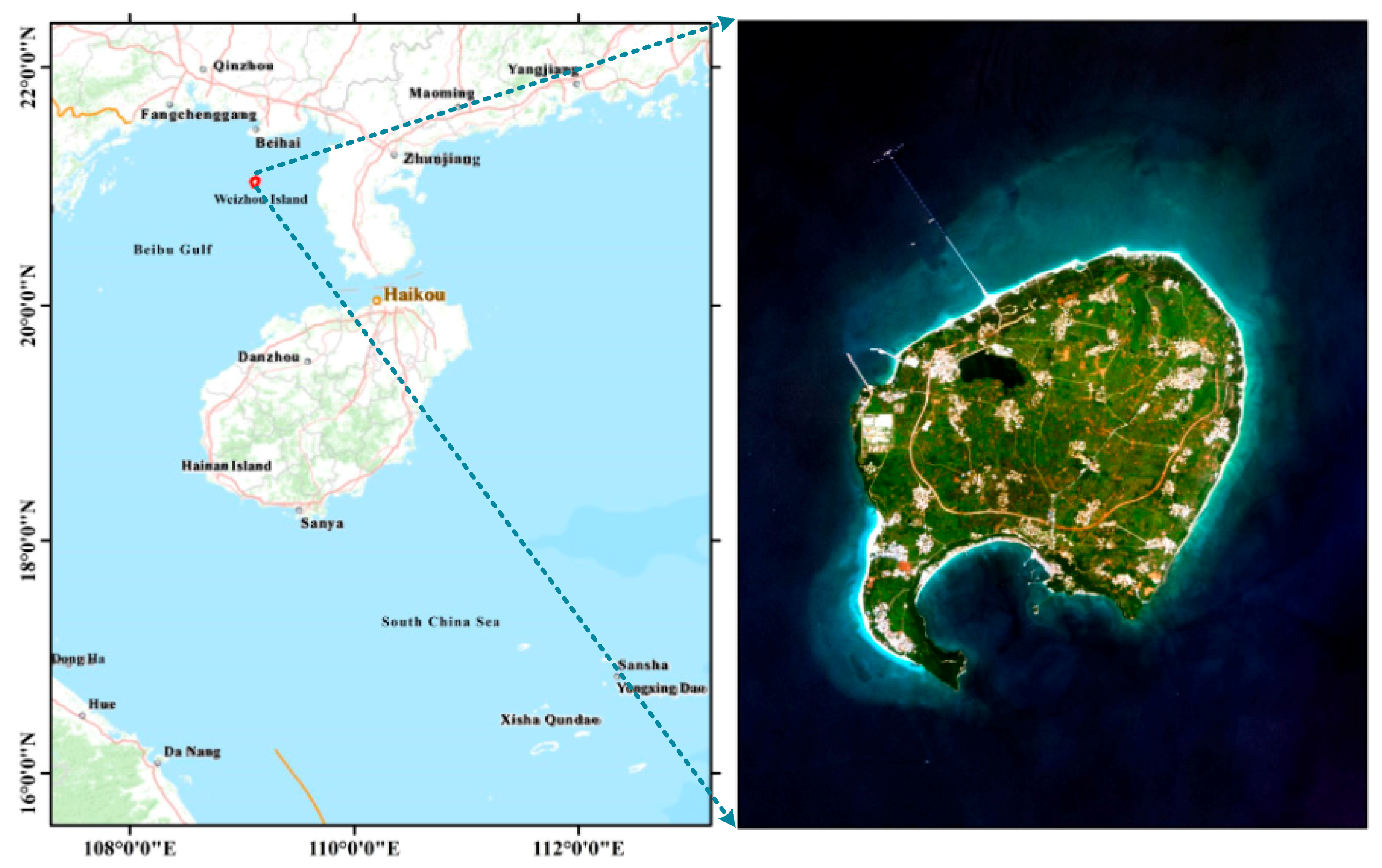
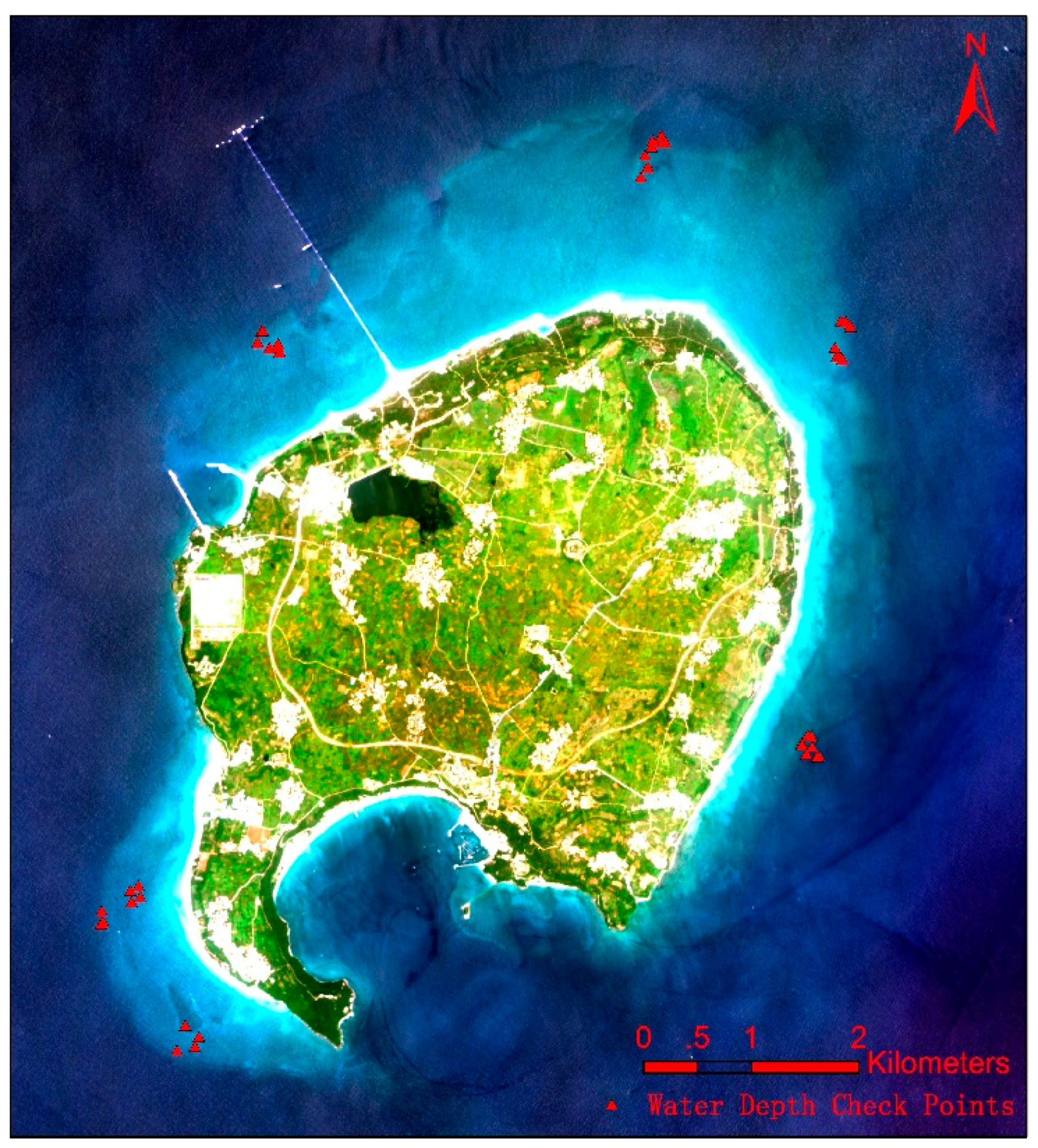
Specifically, Weizhou Island is located at 21°00′–21°05′N, 109°00′–109°10′E, approximately 36 miles from Beihai, Guangxi, as shown in Figure 1. Its coverage area of Weizhou Island is approximately 25 km2. According to Wang et al. [12], the annual average Sea Surface Temperature (SST) and salinity values around Weizhou Island are about 24.55 °C and 31.9‰, respectively, thus it is ideal for coral growth even though the seawater transparency varies only from 3.0 m to 10.0 m [12]. Coral reefs have developed around Weizhou Island since the mid-Holocene, and these reefs cover an area of approximately 6–8 km2 [13,14]. These coral reefs have long been the focus of studies analyzing the responses of coral to global warming and human disturbances, because they are located in a relatively high-latitude area and are heavily influenced by anthropogenic activities [12,14,15,16].
Within this study area, we expect to improve remote sensing data-based solutions for multispectral images to attain relatively accurate and reliable water depth estimations that may be applied to remote, large, or dangerous areas in the future. In addition, another practical motivation of this paper is to provide bathymetric results that will enhance future research of the effects of ambient environmental conditions on the coral reef of Weizhou Island itself.
2. Related Works
In this paper, we mainly focus on band combination methods and semi-analytic methods to make the proposed approach as effective, practical, and convenient as possible. Some related works are summarized as follows.
Based on the law that light is attenuated exponentially with depth in the water column, as follows:
Lyzenga et al. [17,18] argued that the ratio of bottom reflectance between two bands is constant over a given scene for all bottom types; they demonstrated that errors caused by the presence of different bottom types could be corrected with two bands. Accordingly, the two band and n-band combination algorithms were then proposed for the water property-independent and bottom-reflectance-independent water depth extractions. Similarly, Clark et al. [19] introduced a linear multiband method for shallow water depth extraction, which was tested using bands 1 and 2 of Landsat TM imagery acquired in the vicinity of Isla de Vieques. To further develop an empirical solution for the presence of variable bottom types, Stumpf et al. [1] improved the linear multiband combination methods with a ratio of reflectances with only two tunable parameters.
Although band combination methods have been in use since the early 1970s, until now, they are still found to be useful and applicable because of their simple forms and efficient characteristics. Doxani et al. [20] evaluated the effectiveness of several band combination bathymetry algorithms via using a high spatial and spectral resolutions of WorldView-2 (WV-2) image. Yuzugullu and Aksoy [21] compared the linear regression model with a non-linear regression model to predict the depths in Lake Eymir based on WV-2 multispectral satellite images; their results showed that the non-linear regression model predicted these depths slightly better than the linear model. Papadopoulou et al. [3] used Lyzenga’s band combination methods [17,18] and high-resolution IKONOS-2 image to create digital bathymetric maps of the coastal area of Nea Michaniona, Thessaloniki, in northern Greece. Mohamed et al. [22] improved the linear multiband method by using a fitting algorithm called Ensemble Learning (EL) and obtained better performance and accuracy than those obtained by conventional PCA and generalized linear models. Many other related studies [2,23,24,25] were also found to focus on the improvements, comparisons, and applications of these algorithms.
Even though band combination methods are simple enough to have been widely applied by many previous studies, they are obviously highly dependent on field data, which are used for the derivation of the model coefficients. As a result, semi-analytic models were further developed and applied to overcome the disadvantages of the band combination methods by considering such factors as the Inherent Optical Properties (IOPs) of water, bottom types, and in-water light transfer.
Assuming that the water quality and bottom substratum are homogeneous, Bierwirth [26] outlined a method that unmixed the exponential influence of depth in each pixel by employing a mathematical constraint, which was applied in the analysis of Landsat TM data from Hamelin Pool in Shark Bay, Western Australia. Kutser et al. [27] have proved that the bottom type and water depth of the Australian Great Barrier Reef (GBR) can be simultaneously mapped by matching the Hyperion at-sensor radiance data to the simulated at-sensor spectral library. Lafon et al. [28] proposed a semi-empirical bathymetric methodology based on the Hydrolight Radiative Transfer code, which was calibrated using in situ bottom reflectance and effective attenuation coefficient measurements and then applied to determine the depth from SPOT images and to develop topographic maps of the tidal inlet of Arcachon. Lee et al. [29,30,31] also developed a semi-analytical method for shallow water depth estimation using an inversion-optimization approach, which can simultaneously derive the water depth and water column properties from the hyperspectral data in coastal waters. Brando et al. [4] further enhanced the physics-based inversion-optimization approach that was developed by Lee et al. [29,30,31]. They further considered the concentrations of optically active constituents in the water column, different types of substratum covers, and the contribution of every substratum to the remote sensing signal in their enhanced approach. With Lee’s semi-analytic forward model for shallow water remote sensing reflectance, Hedley et al. [32] was able to map water depths efficiently via the introduction of an Adaptive Look-Up Tree (ALUT). Knudby et al. [11] further applied this ALUT method to Landsat 8 data for producing the bathymetric maps for shallow waters in Canada. Recently, Hedley et al. [33] further presented a method for mapping the water depths and the leaf area index (LAI) of seagrasses according to the idea that variations in reflectance is caused by leaf length, leaf position, sediment coverage on leaves, water depth, and solar zenith angle, etc. Sylvain et al. [34] also presented a novel statistical semi-analytic method for mapping water depth and water quality using hyperspectral remote-sensing data, which is based on local maximum likelihood (ML) estimation performed on subimages. The authors assumed that deep water bottom is locally flat so that the spatial correlation between neighboring pixels can be considered sufficiently during the water depth estimation. This method is able to provide multi-resolution maps, where the resolution depends on local water depth.
Semi-analytic methods are usually regarded to be independent of field water depth measurements and having a wider scope of applications than band combination methods. However, many semi-analytic methods were originally developed for high resolution hyperspectral images, e.g., when Dekker et al. [35] reviewed and compared the performances of an empirical and five different analytic/semi-analytic methods, airborne hyperspectral data (Ocean PHILLS and CASI-2) was applied in the experiments. Thus, it is still currently difficult to declare that semi-analytic methods are able to completely solve all bathymetric problems, including those associated with the remote sensing images themselves, especially for the multispectral satellite images that are currently being collected.
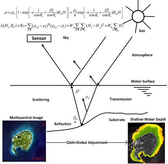
For example, according to a radiative transfer model that can connects the water-leaving reflectance of the optically deep waters , the bottom reflectance , the diffuse attenuation coefficient of the water column , and the water depth to the water-leaving reflectance as follows [36,37]:
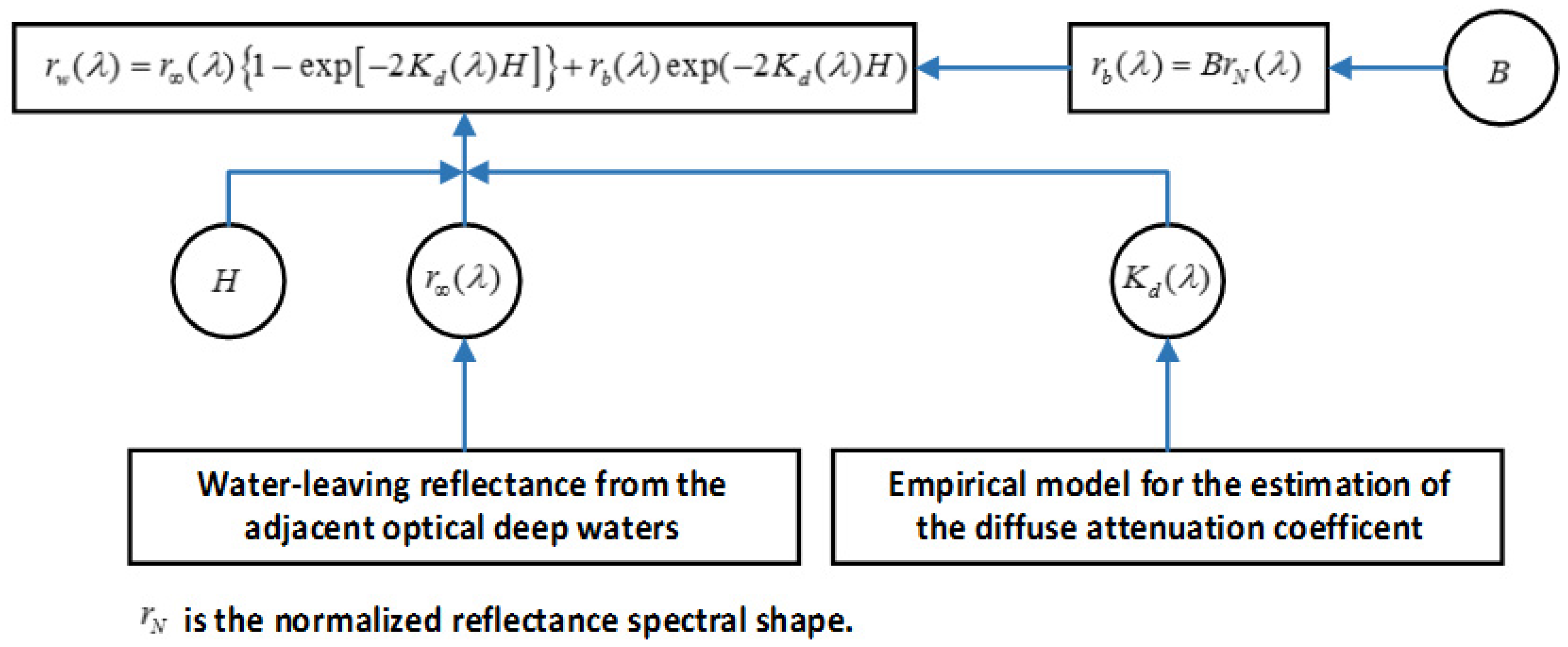
Hu et al. [37] developed a semi-analytic method to derive the coastal water depths of the South China Sea islands using Landsat TM and ETM+ images. In this method, the diffuse attenuation coefficient of the water column is estimated from the adjacent optically deep waters by using the empirical model of MODIS or Landsat data for Case I water, as shown in Figure 2.
On the one hand, when this approach is applied to other types of satellite images, another empirical model need to be built for the estimation of the diffuse attenuation coefficient by using the optically deep water pixels selected from the surrounding areas. Otherwise, when other auxiliary datasets, e.g., MODIS, are needed for the estimation of the diffuse attenuation coefficient, we must ensure that the gap between the acquisition time of the multispectral satellite image and that of the auxiliary data is small enough. On the other hand, this model ignores the influence of the subsurface solar zenith angle , the subsurface view angle , the variations of the bottom reflectances, as well as the differences between the diffuse attenuation coefficients for downwelling and upwelling light.
A more accurate and typical radiative transfer model was developed by Lee et al. [29]. The expression constructs the relationships between the subsurface remote-sensing reflectance for optically deep waters , the bottom irradiance reflectance , the water depth , and the subsurface remote-sensing reflectance as follows:
where and are the optical path-elongation factors for scattered photons from the water column and the bottom, respectively, is the diffuse attenuation coefficient. Some important semi-analytic bathymetric methods have been developed mainly based on the optimization of this model [30,38].
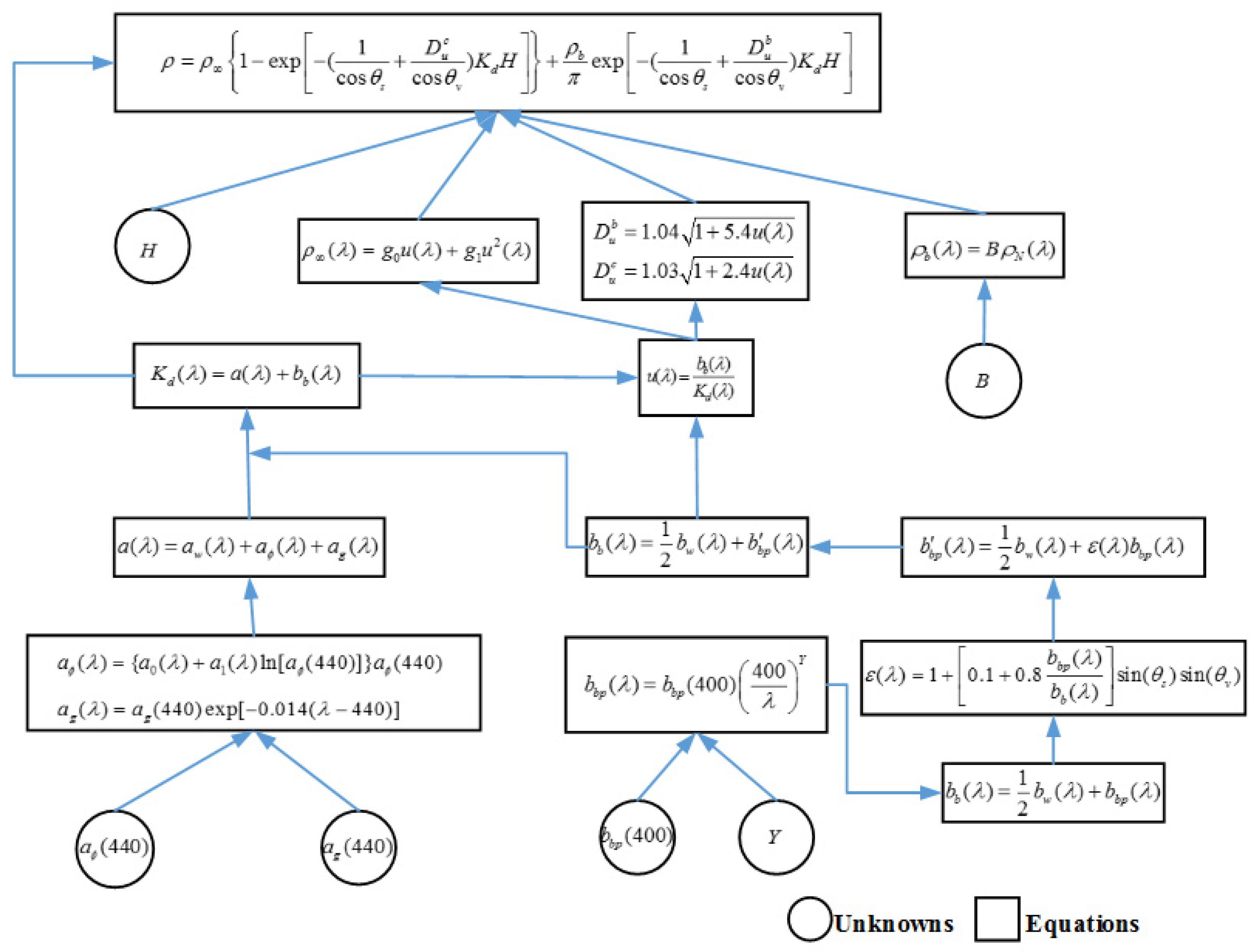
For example, the semi-analytic bathymetric model developed by Eugenio et al. [38] can be summarized as shown in Figure 3. Specifically, the optimum values of , , , , and are determined by minimizing the differences between the observed subsurface remote-sensing reflectance and the estimated reflectance, where is the attenuation coefficient for phytoplankton at 440 nm, is the attenuation coefficient for gelbstoff at 440 nm, is the backscattering coefficient for particles at 400 nm, is the spectral shape that depends on the particulate shape and size, is the bottom albedo at 550 nm, and is the water depth. This approach requires researchers to first initialize the parameter by applying the ratio algorithm, and then, to solve the nonlinear Model (3) using the Levenberg–Marquardt method.
Because the ratio algorithm is used for the initialization, this approach can barely function without the incorporation of field water depth data. In addition, many multispectral satellite images can provide only 3–4 visible wavebands, except for a few types of multispectral satellites (such as WV-2/3 can provide 6 visible wavebands). Hence, the model can become ill-posed because it contains six unknowns for each image pixel, which is usually more than the number of the visible wavebands.
To meet the requirements of most current multispectral satellite images, this paper develops a bathymetric approach on the basis of Model (3). In contrast to the band combination methods and the previously proposed semi-analytic methods, this study mainly highlights the following aspects: (a) making the approach independent of other auxiliary data, such as field water depth measurements and the production of MODIS diffuse attenuation coefficients; (b) reducing the number of unknowns so that the approach can satisfy most current multispectral satellite images; and (c) refining the estimated global water depths to smooth the final water depths and improve the accuracies. The specific details of this approach are discussed in the following sections.
3. Materials and Methods
3.1. Overview of the Approach
In this study, a Quasi-Analytical Algorithm (QAA) is firstly applied to some adjacent optically deep waters to estimate the diffuse attenuation coefficient and the optical path-elongation factors and . As a result, the number of unknowns in the semi-analytic Model (3) is reduced from six (, , , , , and ) to two ( and ). Then, the shallow water depths can be further estimated by using an optimization without the diffuse attenuation coefficients being empirically estimated at first. This choice can also make the method completely independent of field water depth measurement data. Thereafter, we further attempt to propose a global adjustment method to refine the base of the estimated water depths depending on the following two conditions: (a) most of the water depths observed between a pixel and its adjacent pixels should be similar to each other; and (b) if the resolution of the image is high (being better than 5.8 m for the experiments), most of the water depths of the pixels that are close to the transient coastline should be approximately zero. In previous studies, these global adjustments have rarely been taken into consideration. Figure 4 shows the framework of the approach in detail.
3.2. Materials and Preprocessing
3.2.1. Experimental Data
Our experimental data consists of ZY-3 and WorldView-3 (WV-3) multispectral satellite images with 4 and 8 bands, respectively, as shown in Figure 5.
The ZY-3 satellite was launched on 9 January 2012 and represents the first civil high-resolution optical transmission surveying and mapping satellite of China. It is equipped with four optical cameras, including a nadir panchromatic Time Delay and Integration (TDI) CCD camera with a ground resolution of 2.1 m, two back/forward sight panchromatic TDI CCD cameras with a ground resolution of 3.6 m, and a nadir multispectral camera with a ground resolution of 5.8 m. The ZY-3 images are geo-referenced in the World Geodetic System (WGS-84). The geo-positioning accuracy is higher than 14.0 m without ground control after undergoing the on-orbit geometric calibration [39]. In addition, the images have a signal-to-noise ratio (SNR) of approximately 42 [40,41]. The ZY-3 multispectral image chosen as one of the remote sensing data sources for these experiments was acquired on 24 August 2015, at a corresponding tide height of 3.660 m. The satellite azimuth angle and zenith angle are 17.0° and 6.6°, respectively. The sensor band information of the multispectral sensor is presented in Table 1.
The WV-3 satellite was launched by DigitalGlobe Inc., Longmont, CO, USA on 13 August 2014. The WV-3 satellite sensor is a high-resolution commercial satellite sensor operating at an altitude of 617 km. It provides panchromatic, multispectral, short-wave infrared, and CAVIS images with resolutions of 0.31 m, 1.24 m, 3.7 m, and 30 m, respectively. The WV-3 multispectral image used in our experiments was acquired on 1 October 2015, at a corresponding tide height of 2.305 m. The satellite azimuth and zenith values are 218.3° and 21.1°, respectively. The geo-positioning accuracy is predicted to be higher than 3.5 m CE90 without ground control [42]. The WV-3 multispectral images consist of 8 different wave bands (the Coastal, Blue, Green, Yellow, Red, RedEdge, Near-IR1, and Near-IR2 wave bands). The wavelength and the radiometric calibration coefficient information can be all found the IMD file of the WV-3 data.
Moreover, when we performed ecological investigations of the coral reefs around Weizhou Island in October 2015, we measured the water depths at 45 points around the survey stations, as shown in Figure 6. The water depths were measured using an SM-5A hand-held portable depth sounder with an accuracy of 0.1 m, and the horizontal positions were mapped using a Magellan eXplorist 610 hand-held GPS navigation instrument with an accuracy of 3 m. Therefore, the measured water depths can be matched to the satellite data by using the measured horizontal positions and the geo-referenced information of the images.
In this study, these water depths were used to determine the accuracy of the proposed bathymetric approach after the influence of the tidal levels was eliminated. More specifically, all the measured water depths are subtracted by the corresponding tide heights before the accuracy assessment, as well as the water depths estimated from the experimental images. However, when the water depths estimated from the two experimental images are compared with each other, we selected the tide level of the ZY-3 image as a reference, and then corrected water depths estimated from the WV-3 image to this reference. As the tide height corresponding to the ZY-3 image is greater than the one corresponding to the WV-3 image, negative water depths can be then avoided in the comparisons by choosing such a reference.
3.2.2. Data Preprocessing
To implement the bathymetric approach, four main preprocessing steps of the multispectral imagery must be performed prior to obtaining the water depth estimation; these steps include the radiometric calibration, the atmospheric correction, the sunglint correction, and the subsurface remote sensing reflectance estimation.
Radiometric Calibration
The radiometric calibration is performed to transform the Digital Numbers (DN) into the Top-Of-Atmosphere (TOA) radiance .
For the WV-3 image, this calibration is performed with the following equation:
where and are the abscalfactor and the effective bandwidth from the IMD file of the WV-3 data, respectively, and and are both provided by data from the DigitalGlobe website [43].
For the ZY-3 image, the calibration is easy to implement by using the radiometric calibration coefficients shown in Table 1 as follows:
Atmospheric Correction
The atmospheric correction aims to transform the TOA radiance into the top-of-canopy reflectance . Similar to the study of Eugenio et al. [38], the atmospheric correction can also be performed by using the Second Simulation of a Satellite Signal in the Solar Spectrum (6S) radiative transfer code [44,45,46]. Specifically, the can be estimated by using the following equations:
where , , and are the atmospheric correction coefficients calculated by the 6S code.
However, the aerosol optical thickness is also needed to run the 6S code, in addition to the spectral response functions of the sensor bands, the view zenith and azimuth angles, the sun zenith and azimuth angles, the date and time of the image acquisition, and the latitude and longitude of the center of the image scene.
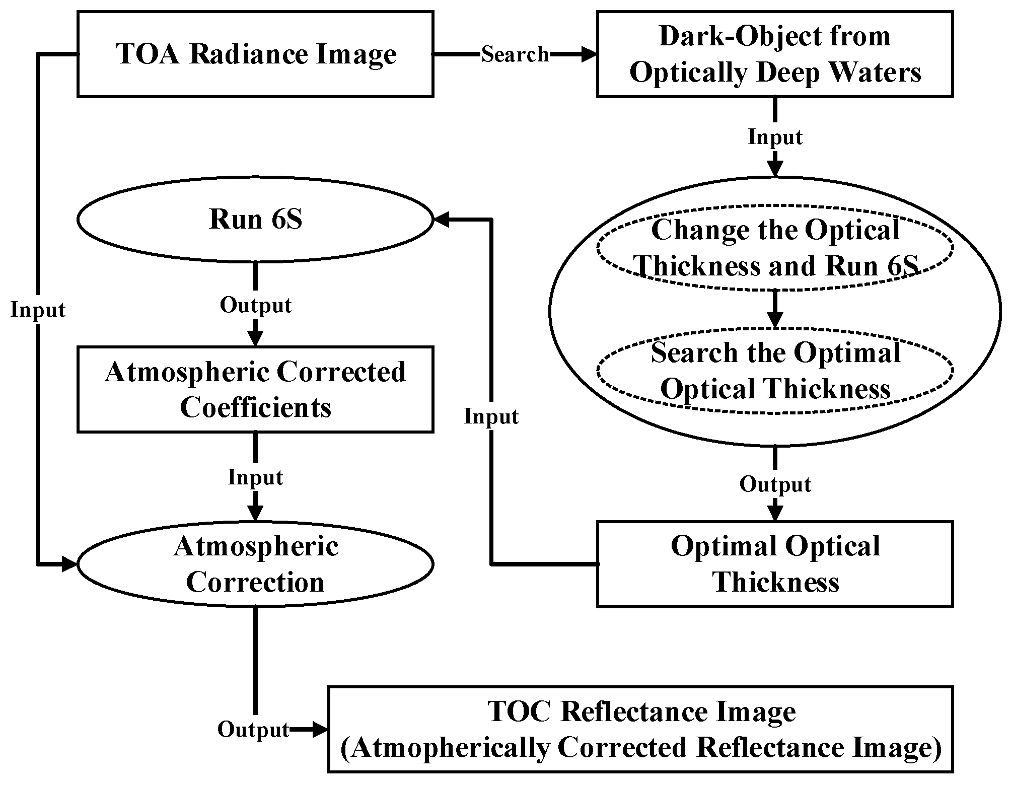
In accordance with Tian et al. [47] and Zheng et al. [48], we first select the minimum TOA radiance of the adjacent optically deep waters to be the dark-object in this study. Then, we change the aerosol optical thickness from 0.0 to 2.0 in intervals of 0.001 and run the 6S code for each of the aerosol optical thicknesses. Consequently, the radiance of the dark-object is transformed into different values of corresponding to different aerosol optical thicknesses by using Equation (6), which allows us to select the aerosol optical thicknesses that cause the of the near-infrared bands (Near-IR1 and Near-IR2 for WV-3 and Near-Infrared for ZY-3) to become as close as possible to zero (which is the optimal aerosol optical thickness).
Thereafter, the optimal aerosol optical thickness is then input into the 6S code to obtain the atmospheric correction coefficients. Therefore, the image can finally be calculated by using Equation (6). The atmospheric correction approach is briefly presented in Figure 7.
Sunglint Correction and Subsurface Remote Sensing Reflectance Estimation
Because we actually use the remote sensing reflectance rather than the TOC reflectance in further processing, must be further transformed into the remote sensing reflectance. As the 6S code can also directly provide the values of solar irradiance and atmospheric diffuse irradiance , we can approximate the remote sensing reflectance using the following equation [49,50,51,52,53]:
where is the reflectivity of the gas-water interface that can be calculated using the Fresnel reflection formula as follows [49,50,51]:
where and are the view zenith angle and the corresponding refraction angle, respectively.
On the other hand, sunglint is usually caused by the specular reflection of solar radiation on the slopes of the waves of surface winds. Thus, it is difficult to avoid and may seriously influence the bathymetry results, especially for images with high spatial resolution. Fortunately, a sunglint correction algorithm has already been developed by Hochberg et al. [54], and it was improved and used to correct the sunglint of high-spatial-resolution images for the estimation of water depth and diffuse attenuation coefficients by Eugenio et al. [38,55]. Thus, to perform the sunglint correction in this study, we simply applied Eugenio’s method to the remote sensing reflectance image. For convenience, we defined the sunglint-corrected remote sensing reflectance corresponding to the remote sensing reflectance as .
The bathymetric Model (3) provides only the subsurface remote-sensing reflectance , rather than the above-surface remote sensing reflectance . Therefore, we further defined the subsurface remote sensing reflectance obtained from , according to the relationship between the above-surface and subsurface remote sensing reflectances provided by Lee et al. [29,30], as follows:
3.3. Bathymetric Model and Its Solution
3.3.1. Reduce the Number of Unknowns
Many current multispectral satellite images can provide only 3–4 visible wavebands; for example, the ZY-3 imagery in this study provides only three visible wavebands (the blue, green, and red bands). As a result, we must reduce as many unknown variables of the bathymetric model as possible. Otherwise, the bathymetric model may become ill-conditioned, and the approach will end in failure.
According to the work of Prieur and Sathyendranath [56] and Lee et al. [29], the phytoplankton pigment absorption coefficient at 440 nm, , can be further parameterized using the chlorophyll-a concentration as follows:
As illustrated in Figure 3, when Model (3) is used, the backscattering coefficients of the particles can be parameterized, using and , as follows:
To reduce the number of unknown variables, is further updated using the chlorophyll-a concentration (as shown in Appendix A and Appendix B) as follows:
where , and
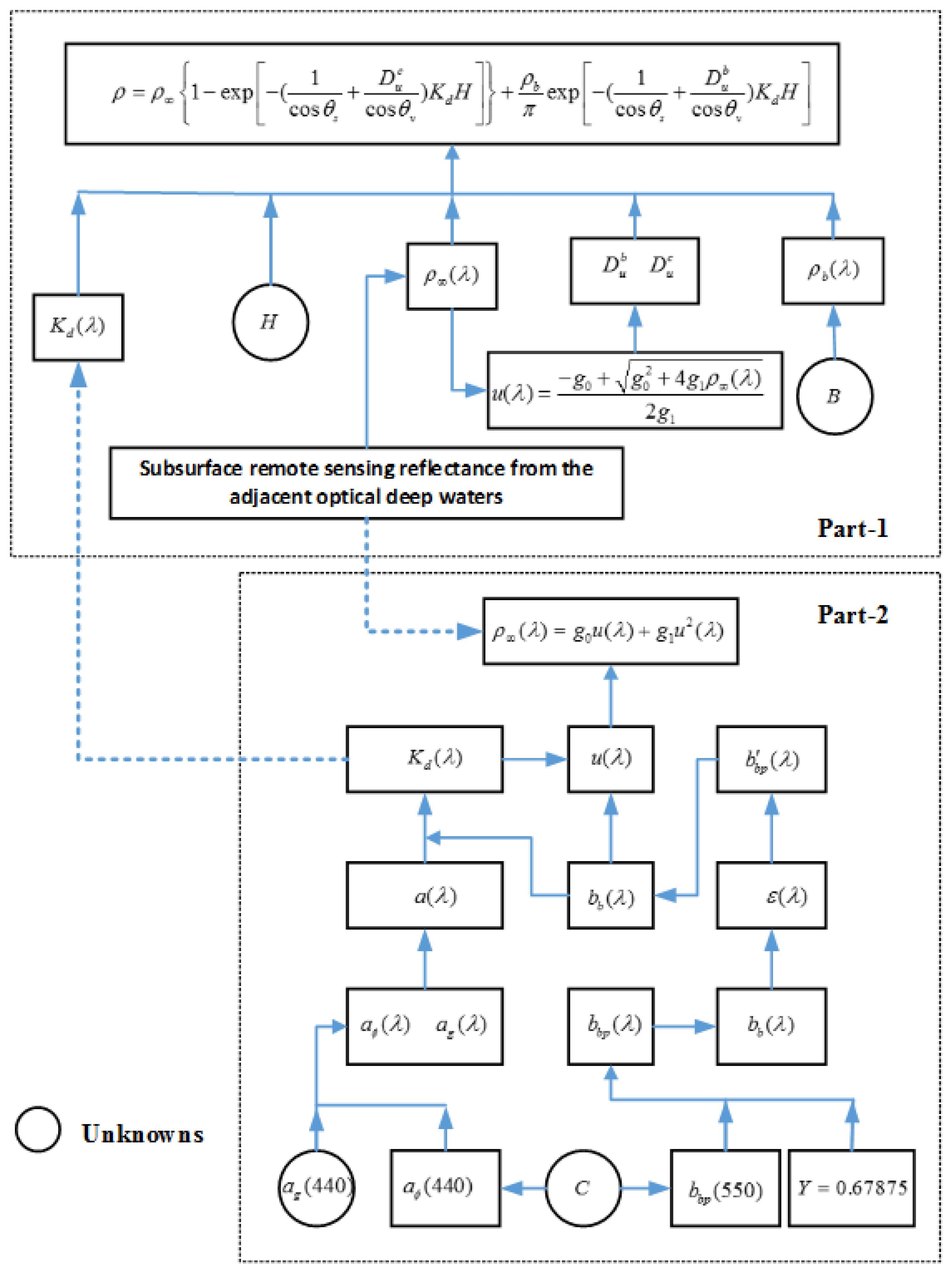
To summarize, the model described in Figure 3 can now be updated using Equations (10), (12), and (13), and a constant of . As a result, the number of unknown variables is reduced to only four: , , , and .
To further reduce the number of unknowns, we note that
can be rewritten as
Therefore, we can further separate the updated semi-analytic bathymetric model into two parts, as shown in Figure 8. In other words, we can solve the bathymetric problem with the following two steps: (a) according to Part 2 of the updated semi-analytic bathymetric model, determine the optimal values of and , so that the differences between the values of the estimated and the subsurface remote sensing reflectance of the optical deep waters are as small as possible, thus allowing the diffuse attenuation coefficient to be estimated; and (b) according to Part 1 of the updated semi-analytic bathymetric model, determine the optimal values of and for every pixel, so that the differences between the values of the estimated subsurface remote sensing reflectance and the observed values calculated by Equation (9) are as small as possible. We will illustrate these two steps in the following two sections, respectively.
3.3.2. Solve the Diffuse Attenuation Coefficient
Eugenio et al. [55] adapted the QAA for WV-2 multispectral images to estimate the values of phytoplankton attenuation , gelbstoff and detritus attenuation , and particle backscattering . In this study, we present a similar approach to the adjacent optically deep waters according to Part 2 of the updated semi-analytic bathymetric model (Figure 8). In contrast to Eugenio et al. [55], our model is parameterized using and , which can be applied to multispectral images that have no fewer than 2 visible bands.
Specifically, to solve the parameters of and , we first change from 0 m−1 to 0.5 m−1 using intervals of 0.001 m−1, then change from 0.1 mg/m3 to 5.0 mg/m3 using intervals of 0.1 mg/m3, and calculate the corresponding subsurface remote sensing reflectance of each pair of and using Part 2 of the updated semi-analytic bathymetric model (Figure 8). Then, the initialization of the values of and are selected by making the sum of squared differences between the calculated subsurface remote sensing reflectance and the observed reflectance to be as close to zero as possible. Thereafter, the Levenberg–Marquardt method is used to solving for the optimal values of and . Finally, the average diffuse attenuation coefficient is then estimated from these optimal and values, according to Part 2 of the updated semi-analytic bathymetric model (Figure 8). The estimated here is thus assumed to be known and is input into Part 1 of the model to complete the following steps of the proposed approach.
The effectiveness of the frame of the QAA approach has already been proved by Eugenio et al. [55], so we only need to further argue that the estimated diffuse attenuation coefficient here is approximately constant in the study area for each of the two experimental images.
To prove this, several deep-water regions were first designated manually from the two experimental images. Then, 100 pixels were randomly selected from the designated regions. The diffuse attenuation coefficients corresponding to these pixels were finally estimated by using our approach. The statistical analyses of these results are shown in Table 2 and Table 3, as follows.
In Table 2 and Table 3, the standard deviation of the diffuse attenuation coefficient is comparatively small, as are the values of skewness and kurtosis. This means that the diffuse attenuation coefficients estimated from most deep-water pixels are close to their means. In other words, the diffuse attenuation coefficients obtained from both the WV-3 image and the ZY-3 image prove to be approximately constants.
3.3.3. Initialize the Water Depths
The bottom irradiance reflectance is usually expressed as follows [30,37,38]:
where , which is usually assumed to be known in most bathymetric approaches, is the spectral shape of the reflectance normalized at the reference wavelength. For example, Lee et al. [30] and Eugenio et al. [38] used a 550-nm-normalized sand-albedo shape, and Hu et al. [37] tried to derive from the spectral reflectance values of sand, algae, dark sediment, and their mixtures.
To estimate water depths using Part 1 of the updated semi-analytic bathymetric model (Figure 8), we must also specify the shape of prior to running our bathymetric approach. Equation (3) illustrates that if the water depth is close to zero, the subsurface remote sensing will be approximately equal to
Therefore, we manually select several typical subsurface remote sensing reflectance shapes located close to the transient coastline as references. We assign these subsurface remote sensing reflectance shapes values of (), where is the number of selected reference shapes. Considering that the water depths of the selected shapes are not actually equal to zero, we parameterized the bottom irradiance reflectance shapes according to Equation (17), as follows:
or
Thereafter, in principle, we can estimate pixel-by-pixel water depths according to Part 1 of our updated semi-analytic bathymetric model (Figure 8) using the Levenberg–Marquardt algorithm. However, the initialization of the water depth must be performed prior to applying the Levenberg–Marquardt algorithm. In this study, the initial values of and are estimated using the following steps:
(a) For each value of (), change from 0 m to 40 m using intervals of 0.5 m, change from 0.5 to 1.5 using intervals of 0.01, and calculate the subsurface remote sensing reflectance corresponding to every pair of and according to Part 1 of the model, as shown in Figure 8.
(b) For each value of , build a K-D tree [57] based on the calculated subsurface remote sensing reflectance , and define this K-D tree as , where K-D tree is known as a space-partitioning data structure for organizing points in a k-dimensional space, and it was useful for us to efficiently search the closest reflectance of the observed one from these calculated ones in the following step.
(c) For each observed value of subsurface remote sensing reflectance (calculated by Equation (9)), determine its closest corresponding reflectance value from , define the result as , and define the corresponding square distance as .
(d) For each observed value of subsurface remote sensing reflectance , determine the minimum distance from the set of , define the result as , and define the corresponding normalized reflectance spectral shape as .
As a result, the value of is selected as the normalized reflectance spectral shape corresponds to the observed . Furthermore, based on such normalized reflectance spectral shape, the values of and corresponding to are selected to initialize the Levenberg–Marquardt algorithm. Finally, the result of the Levenberg–Marquardt algorithm is then used as the initialization to perform the following global adjustment.
3.4. Global Adjustment of Water Depths
In contrast to most bathymetric methods, we further propose a global adjustment method to refine the estimated water depths, for trying to smooth the water depths and improve the accuracies.
As mentioned in Section 3.1, the principle is based on the following two conditions: (a) most water depths should be close to each other for any two adjacent pixels; and (b) if the pixel size is small, most water depths of the pixels that are close to the transient coastline should be approximately zero. The specific computational model is described as follows.
First, we define the water depth and the parameter of a given pixel as and , respectively, and define the corresponding normalized reflectance spectral shape (see Section 3.3.3) as . As a result, Condition (a) can be described as follows:
where represents one pixel that is adjacent to pixel . In addition, if pixel is located close to the transient coastline, then Condition (b) can be described as follows:
Therefore, by considering Part 1 of the updated semi-analytic model (Figure 8) together with Equations (20) and (21), we can construct the following objective function to refine the estimated water depths:
where represents the region of the image that is used to perform the bathymetric approach, is the adjacent pixel set of in region , and is the pixel set where the water depths are close to zero. In this study, consists of pixels that are located close to the transient coastline (at a distance of less than two pixels); is the observed subsurface remote sensing reflectance vector calculated by Equation (9); and is the subsurface remote sensing reflectance vector expressed by Equation (3), which is dependent on the unknown parameters and . and are the weights of the corresponding items of the objective function. can usually be determined according to the observed local variations in the water depths; if the actual variation in the water depth is large, then should be set to a relatively small positive number. To avoid the over-smoothing of the water depths, we set to a small number in these experiments, i.e., . is used to constrain the water depths of the pixels around the transient coastline to be as close to zero as possible; thus, in this study, .
The first item of the objective function causes the results to fit the radiative transfer Model (3) as closely as possible. The second item is a smoothing item, which can reduce the influence of noise on the final water depth results. When it is difficult to determine the pixels with water depths of approximately zero, the third item of the objective function can be ignored in the global adjustment approach.
In principle, all values of the water depth and the parameter can be globally adjusted by minimizing the proposed objective function. Specifically, we started at the values of water depth and parameter that were estimated in Section 3.3.3 and employed the trust–region–reflective method proposed by Coleman and Li [58,59] to optimize the objective function in this study.
Note that in case of some pixels that are close to the transient coastline but are not really zeroes in depth, we should discard such pixels from before performing the global adjustment.
4. Results
We have already applied the proposed bathymetric approach to the two experimental images that were shown in Section 3.2.1. Accordingly, the results will be illustrated and discussed in the following sections.
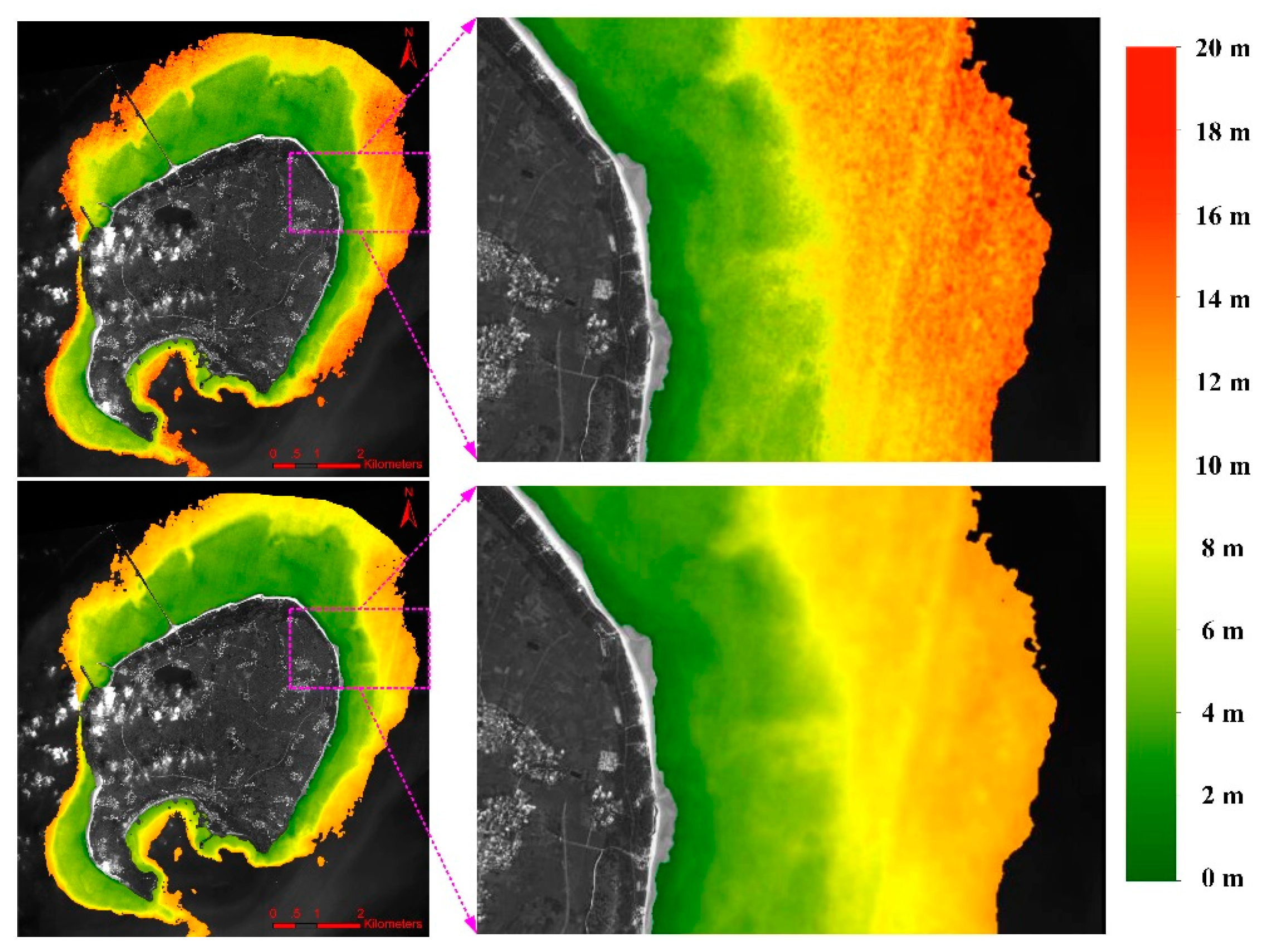
4.1. Visualization of the Water Depths
4.2. Evaluations of the Accuracies before and after the Global Adjustment
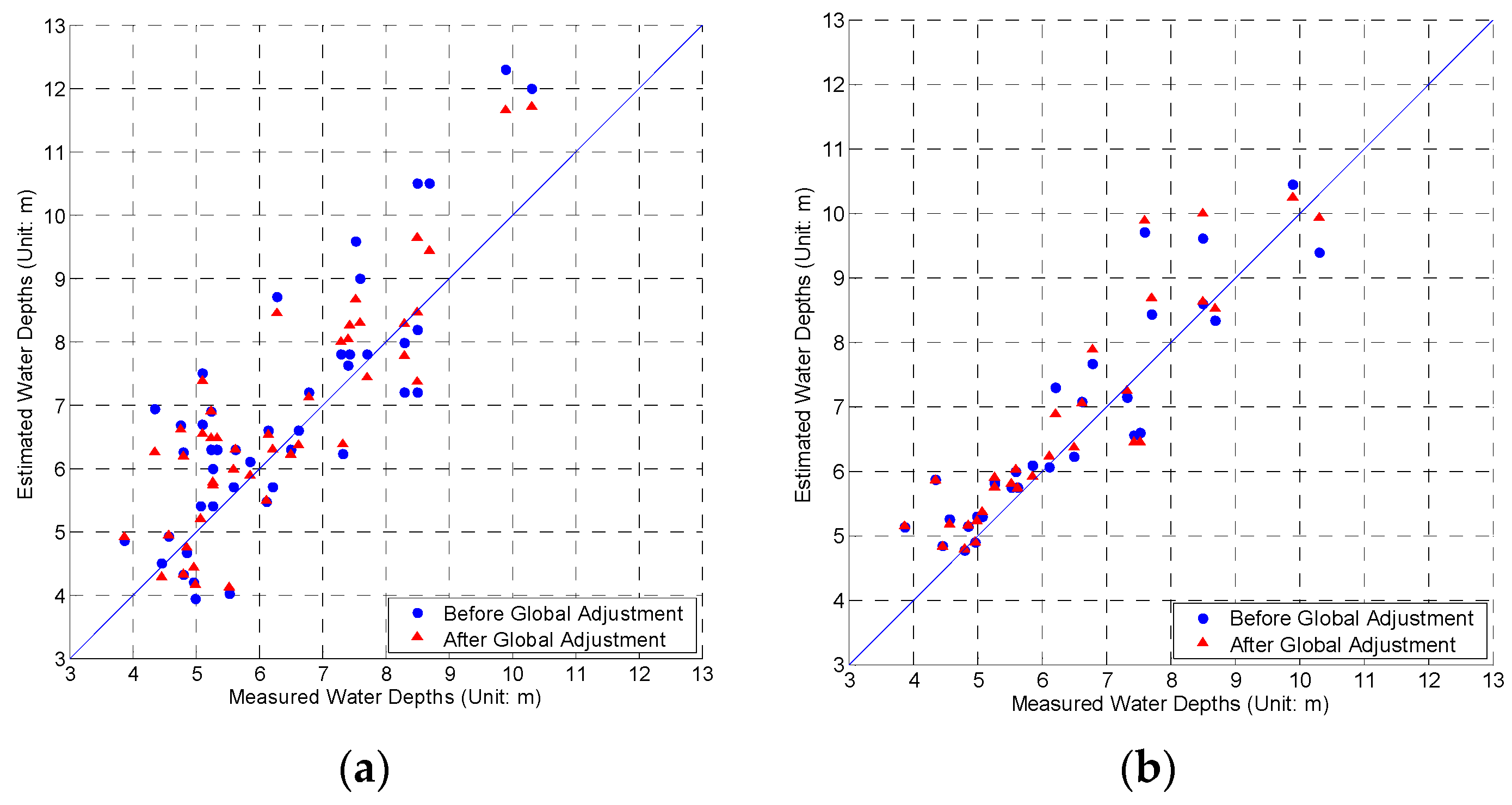
Since water depths at 45 points around the Weizhou Island have been measured during October 2015, the accuracy of the proposed bathymetric approach can be then evaluated by comparing the estimated water depths with the measured ones. These comparisons are shown in Figure 11, and the corresponding statistics are illustrated in Table 4.
It should be note that although the gap between the time that the ZY-3 image was obtained and the water depth measurements were acquired was approximately 40 days, the water bottom around Weizhou Island changed little during this time due to the following three reasons: (a) no very strong tropical storms passed through Weizhou Island during this time; (b) the island is piled up under the water when Quaternary basalt magma gushed out, and now has a relatively stable structure [60]; and (c) the distributions of the water depths estimated from the two images were seen to be similar to each other, as is seen in the visualization of Section 4.1.
4.3. Comparisons between the Water Depths Estimated from the Two Different Images
In contrast to other works, we compared the differences between the water depths estimated from the ZY-3 and the WV-3 images for further testing the performances of the proposed approach. Specifically, we randomly selected 200 points from the two images and quantitatively compared the results obtained from these two images. The results are shown in Figure 12. When the statistics are further estimated, we find that the maximum value of the absolute errors (MAX) is 4.69 m, the mean of the absolute errors (MAE) is 1.02 m, and the root mean square error (RMSE) is 1.24 m, where the errors are calculated by using the differences between the water depths estimated from the ZY-3 and the WV-3 images.
5. Discussion
5.1. Discussion on the Visualization of the Water Depths
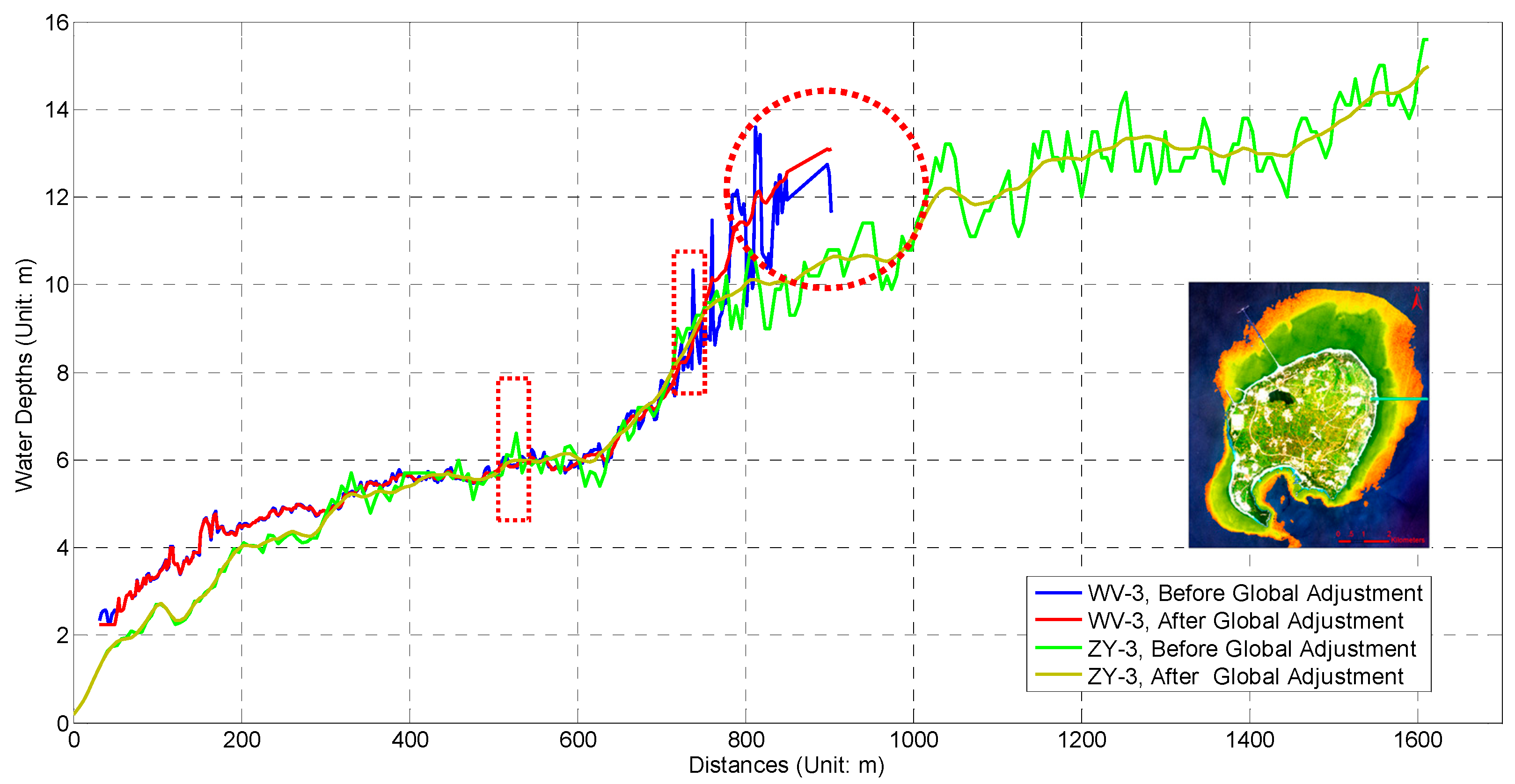
We can see from Figure 9 and Figure 10 that the water depths are slightly smoother after the global adjustment, especially for the ZY-3 image. To more carefully compare the water depths obtained before and after the global adjustment, we further examined an arbitrary transect of water depths shown in Figure 13.
When comparing only the water depths obtained before and after the global adjustment for the ZY-3 image and the WV-3 image, the water depths along the transect are smoother after performing the global adjustment, as shown in Figure 13.
Note that the ZY-3 image has a lower SNR, and this may be the reason why the smoothing effect of the ZY-3 image was more significant than the WV-3 image.
On the other hand, the following aspects are also illustrated in Figure 13: (a) when the water depths are less than 5 m, the water depths estimated from the WV-3 image are slightly greater than those estimated from the ZY-3 image, although most of these differences are less than approximately 1 m; (b) when the water depths range from 5 m to 10 m, the water depths obtained from the two different images agree well with each other; and (c) when the water depths are more than 10 m, the differences between the two images may reach up to 2 m (see the dotted circle in Figure 13).
When the water depths are lower than 5 m (i.e., about 2 m without tide corrections), the proposed approach may be more susceptible to the errors of the spectral shape of the selected bottom reflectance. This is regarded as the reason why the differences between the water depths estimated from the two images become slighter and slighter as the water depths increase until about 10 m, as shown in Figure 13.
As can also be seen in Figure 13, before the global adjustment, the local variations in water depth increase with increasing water depth. This is due to the decreases in the ratio between the radiations reflected by the water bottom and those coming from the water column. Thus, the influences of the noise become increasingly significant, so that the local variations of water depths become large, as do the differences between the water depths estimated from the two images as seen in the dotted circle of Figure 13.
Besides, we note that the ZY-3 and the WV-3 images are acquired at 11:23 a.m., 24 August 2015, with the sun zenith angle of 22.1°, and 11:37 a.m., 1 October 2015, with the sun zenith angle of 27.6°, respectively. Hence, the WV-3 image may correspond to a weaker direct solar radiation intensity than the ZY-3 image. This can also cause the local variations of the water depths estimated from the WV-3 image being greater than the ZY-3 image at the places where the water depths are deeper than 10 m, as shown in the dotted circle of Figure 13.
5.2. Discussion on the Accuracy Assessment of the Estimated Water Depths
Except for the visualization results, we focus more on the quantitative statistics of the differences between the estimated and measured water depths.
As shown in Figure 11, the water depths estimated for the ZY-3 image appear to be closer to the measured depths after undergoing the global adjustment sub-approach, but this trend is not remarkable for the WV-3 image. This phenomenon is further confirmed by the statistics shown in Table 4: the MAE and RMSE changed from 0.97 m and 1.22 m before the global adjustment to 0.81 m and 1.01 m after undergoing the global adjustment for the ZY-3 image, while from 0.58 m and 0.75 m to 0.56 m and 0.77 m for the WV-3 image.
When Figure 13 was further reviewed, we can clearly find that the proposed global adjustment sub-approach is able to adjust some possible large outliers to the relatively reasonable values, as shown in the dotted boxes of Figure 13. At the same time, we also find that if the variation of the adjacent water depths is not remarkable, the global adjustment sub-approach can hardly influence the final water depth estimation. Accordingly, we speculate that the reasons for the mentioned phenomenon may include the following aspects:
(a) The SNR of the ZY-3 image is lower than that of the WV-3 image; therefore, the influences of noise were more serious for ZY-3 than for WV-3.
(b) The band number of the ZY-3 image is considerably less than that of the WV-3 image; thus, the bathymetry of the ZY-3 image is much more sensitive to noise than that of the WV-3.
(c) The smoothing item of the objective function (see Equation (22)) works well when the noises are sensitive or the influences of the noises are serious.
These factors indicate that the global adjustment sub-approach can not only improve the accuracy when the influences of the noises are remarkable, but can also avoid the over-smoothing of the water depths when the results are not sensitive to the noises. This is what common smoothing filters are difficult to realize.
On the other hand, if we focus only on the statistics after the global adjustment as shown in Table 4, we note that the proposed approach have exceeded those of Hu et al. [37] and Eugenio et al. [38] on RMSEs, as shown in Table 5. Although these RMSEs are calculated by using different images with different resolutions, we are more inclined to believe that they are comparable to each other. The reason is that we can see from Table 5 that Hu et al. [37] obtained better RMSEs (1.1 m and 1.6 m) with 30 m resolution of Landsat ETM+ images than those of Eugenio et al. [38] (1.20 m and 1.94 m) with 2.0 m resolution of WV-2 images, while the bathymetric model used by Hu et al. [37] (see Equation (2)) can be seen as a simplification or an approximation of the one used by Eugenio et al. [38] (see Equation (3)). Actually, we used a ZY-3 multispectral image with a resolution of 5.8 m and a WV-3 multispectral image with a resolution of 1.24 m in the experiments, and obtained the RMSEs of 1.01 m and 0.77 m respectively, which were less than those of Hu et al. [37] and Eugenio et al. [38].
When we further compare the proposed approach with those of Hu et al. [37] and Eugenio et al. [38], we can see that the proposed approach is not only better than other methods on accuracies as mentioned previously, but also has the following advantages:
(a) This approach can extract water depths directly from the multispectral image itself and does not require the use of extra MODIS data, water depth data, or water column data, except for the evaluation of its results;
(b) This approach has fewer variables than many other current methods, which means that it can be used to analyze most current multispectral satellite images, even some images that contain only 2–3 visible wavebands.
Note that the proposed approach reduced the unknown variables through parameterizing the radiative transfer model using only two unknown parameters (see Section 3.3.1) instead of six of Eugenio et al. [38] (see Equation (3) in Section 2). This seems to increase the model errors for the proposed approach, and may lead to the statistics of the differences between the estimated and measured water depths becoming worse, but this is not true as shown in Table 4 and Table 5. Hence, we believe that the parameterization is reasonable without causing significant model errors in this study.
In addition, Figure 12 further demonstrates that these comparisons between the water depths estimated from the ZY-3 and the WV-3 images are similar to the results derived from the transect shown in Figure 13; the results of statistical analysis indicate that the value of the root mean square error is 1.24 m (see Section 4.3).
In fact, we can also estimate the RMSE of the differences between the water depths estimated from the ZY-3 and WV-3 images according to the results shown in Table 4 as follows:
Such value is relatively small and very close to 1.24 m. This indicates that the water depths estimated from the ZY-3 and WV-3 images are consistent to each other, and then is able to further enhance our confidence in the effectiveness and the accuracies of the proposed approach.
5.3. Discussion on Supplementary Notes and Future Work
We note that the global adjustment sub-approach depends slightly on the assumption that most water depths should be similar to each other between one pixel and its adjacent pixels. This may indicate that this method involves an implicit assumption that the detected sea floor elevations are continuous and vary gradually. Thus, when the sea floor is not sufficiently continuous, this refinement may become inaccurate or may even fail. Fortunately, when the weight of the smooth item (the second item of the objective function, Equation (22)) is set as a small value (), we find that the smooth item mainly works when the noises are sensitive or their influences are serious, as discussed in Section 5.2. In other words, when the noises of the images are significantly sensitive or the influences of the noises are serious, the global adjustment approach works well on improving the water depth results, otherwise the global adjustment approach is able to avoid the over-smoothing of the water depths.
As a result, we believe that the proposed global adjustment sub-approach can be applied to estimate the water depth of many types of sea floors. Specifically, the proposed approach has great potential for the marine surveying and mapping of large, remote, or dangerous areas in the future, particularly for further research on the bathymetries of typical coral reefs.
Thus, more different images and regions are needed to further test and improve this approach in our next works. Moreover, we also plan to improve this approach by further considering the variations in the properties of the water column between shallow and deep waters in future studies that may introduce the global adjustment sub-approach to smooth the water-column properties.
6. Conclusions
In this paper, a QAA method is firstly explored to estimate the diffuse attenuation coefficients, and then the parameterization of bathymetric model is further simplified. Based on these two aspects, we have developed a QAA approach that includes sub-approaches of initialization and a novel global adjustment to estimate the water depths around Weizhou Island from multispectral images. One advantage is that the approach is able to reduce the number of unknowns and is independent of auxiliary datasets. Another advantage is that the global adjustment sub-approach can not only smooth the final water depths and improve the accuracies, but can also avoid the over-smoothing of water depths. Experimental results have finally illustrated that the water depths estimated from the ZY-3 and WV-3 images are approximately consistent to each other, and yield EMSEs of 1.01 m and 0.77 m, respectively. Therefore, the proposed approach is thought to be competitive to other QAA bathymetric methods.
Acknowledgments
This work is financially supported by the National Basic Research Program of China (2013CB956102), the National Natural Sciences Foundation of China (91428203), the BaGui Scholars Program Foundation (2014BGXZGX03), and the Natural Sciences Foundation of Guangxi, China (2016GXNSFBA380031). We are very grateful to our colleagues, Professor Zheng Wang and Kun Hu for their precious comments and revision of the language, and special thanks are given to the anonymous reviewers and members of the editorial board for their suggestions of improving this article.
Author Contributions
Kefu Yu, Rongyong Huang, and Yinghui Wang conceived and designed the experiments, and wrote the paper together; Rongyong Huang, Jikun Wang, and Wenhuan Wang performed the experiments; Rongyong Huang analyzed the experimental results; and Lin Mu provided the ZY-3 image and contributed the image pre-processing tool.
Conflicts of Interest
The authors declare no conflict of interest.
Appendix A. The Relationship between Backscattering Coefficients and Wavelengths
As illustrated in Figure 3, when Model (3) is used, the backscattering coefficients of particles are parameterized, using and , as follows:
If we set in Equation (A1), we obtain
hence,
Lee et al. [29] noted that most Hydrolight simulations used a phase function with a ratio of 1.9%, but they made use of another more highly backscattering phase function (with a ratio of 3.7%) in their simulation. Here, we followed the methodology of Lee et al. [29] and assumed that the ratio is independent of in this study. As a result, Equation (A3) can be rewritten as follows:
where represents the backscattering coefficient for the particles.
It should be noted that the parameter is sometimes considered an unknown in some studies, e.g., Eugenio et al. [38]. However, in other studies, is set as a constant. For example, when Eugenio et al. [55] estimated the IOPs using QAA, was set to . In this study, we decided to set to a constant to reduce the number of unknowns in the model. Its value is derived as follows.
If is near , then Equation (A4) can be approximated by using the first-order Taylor’s expansion, as follows:
According to the discussions of Voss [61] and Loisel and Morel [62], when ranges between 440 nm and 670 nm, then can also be parameterized by
If we set in Equation (A6), we obtain
thus,
When Equation (A5) is compared to Equation (A8), it can be found that if
then the right sides of Equations (A5) and (A8) will become equal. In other words, Equation (A8) can be seen as an approximation of Equation (A5).
If we set nm, then , and according to Equation (A4),
Appendix B. The Relationship between the Backscattering Coefficient for Particles at 550 nm and the Chlorophyll-a Concentration
As seen in the studies of Voss [61], Lee et al. [29,30], and Morel and Maritorena [63], among others, for a certain wavelength , the corresponding scattering coefficient for particles can usually be parameterized using the chlorophyll-a concentration . For example, for nm,
As mentioned in Appendix A, we followed the method of Lee et al. [29] and assumed that the ratio is 3.7%, which is independent of the wavelength. Therefore, the backscattering coefficient for the particles can be expressed as follows:
References
- Stumpf, P.; Richard, P.; Holderied, K.; Sinclair, M. Determination of water depth with high-resolution satellite imagery over variable bottom types. Limnol. Oceanogr. 2003, 48, 547–556. [Google Scholar] [CrossRef]
- Su, H.; Liu, H.; Heyman, W.D. Automated Derivation of Bathymetric Information from Multi-Spectral Satellite Imagery Using a Non-Linear Inversion Model. Mar. Geod. 2008, 31, 281–298. [Google Scholar] [CrossRef]
- Papadopoulou, M.; Lafazani, P.; Mavridou, E.R.; Tsakiri-Strati, M.; Doxani, G. Creation of Digital Bathymetric Maps using High Resolution Satellite Imagery and Multispectral Bathymetric Modeling for Shallow Waters. Tour. Manag. 2015, 14, 407–408. [Google Scholar]
- Brando, V.E.; Anstee, J.M.; Wettle, M.; Dekker, A.G.; Phinn, S.R.; Roelfsema, C. A physics based retrieval and quality assessment of bathymetry from suboptimal hyperspectral data. Remote Sens. Environ. 2009, 113, 755–770. [Google Scholar] [CrossRef]
- Mumby, P.J.; Clark, C.D. Benefits of water column correction and contextual editing for mapping coral reefs. Int. J. Remote Sens. 1998, 19, 203–210. [Google Scholar] [CrossRef]
- Moustier, C.D.; Matsumoto, H. Seafloor acoustic remote sensing with multibeam echo-sounders and bathymetric sidescan sonar systems. Mar. Geophys. Res. 1993, 15, 27–42. [Google Scholar] [CrossRef]
- Chen, E.; Guo, J. Real time map generation using sidescan sonar scanlines for unmanned underwater vehicles. Ocean Eng. 2014, 91, 252–262. [Google Scholar] [CrossRef]
- Montereale-Gavazzi, G.; Roche, M.; Lurton, X.; Degrendele, K.; Terseleer, N.; Lancker, V.V. Seafloor change detection using multibeam echosounder backscatter: Case study on the Belgian part of the North Sea. Mar. Geophys. Res. 2017, 38, 1–19. [Google Scholar] [CrossRef]
- Maleika, W. The influence of track configuration and multibeam echosounder parameters on the accuracy of seabed DTMs obtained in shallow water. Earth Sci. Inform. 2013, 6, 47–69. [Google Scholar] [CrossRef]
- Parnum, I.M.; Gavrilov, A.N. High-frequency multibeam echo-sounder measurements of seafloor backscatter in shallow water: Part 1 Data acquisition and processing. Underw. Technol. Int. J. Soc. Underw. 2011, 30, 3–12. [Google Scholar] [CrossRef]
- Knudby, A.; Ahmad, S.K.; Ilori, C. The Potential for Landsat-based Bathymetry in Canada. Can. J. Remote Sens. 2016, 42, 1–34. [Google Scholar] [CrossRef]
- Wang, W.; Yu, K.; Wang, Y. A Review on the Research of Coral Reefs in the Weizhou Island, Beibu Gulf. Trop. Geogr. 2016, 36, 72–79. [Google Scholar]
- Yu, K. Coral reefs in the South China Sea: Their response to and records on past environmental changes. Sci. China Earth Sci. 2012, 55, 1217–1229. [Google Scholar] [CrossRef]
- Yu, K.; Zhao, J. Coral reefs (of the South China Sea). In The South China Sea—Paleoceanography and Sedimentology, 1st ed.; Wang, P., Li, Q., Eds.; Springer: Dordrecht, The Netherlands, 2009; pp. 229–248. [Google Scholar]
- Chen, T.; Li, S.; Yu, K.; Zheng, Z.; Wang, L.; Chen, T. Increasing temperature anomalies reduce coral growth in the Weizhou Island, northern South China Sea. Estuar. Coast. Shelf Sci. 2013, 130, 121–126. [Google Scholar] [CrossRef]
- Chen, T.; Zheng, Z.; Mo, S.; Tang, C.; Zhou, X. Bioerosion in Porites corals at Weizhou Island and its environmental significance. Chin. Sci. Bull. 2013, 58, 1574–1582. [Google Scholar] [CrossRef]
- Lyzenga, D.R. Passive remote sensing techniques for mapping water depth and bottom features. Appl. Opt. 1978, 17, 379–383. [Google Scholar] [CrossRef] [PubMed]
- Lyzenga, D.R.; Malinas, N.P.; Tanis, F.J. Multispectral bathymetry using a simple physically based algorithm. IEEE Trans. Geosci. Remote Sens. 2006, 44, 2251–2259. [Google Scholar] [CrossRef]
- Clark, R.K.; Fay, T.H.; Walker, C.L. A Comparison of Models for Remotely Sensed Bathymetry; Naval Ocean Research and Development Activity: Stennis Space Center, MS, USA, 1987. [Google Scholar]
- Doxani, G.; Papadopoulou, M.; Lafazani, P.; Pikridas, C.; Tsakiristrati, M. Shallow-Water Bathymetry over Variable Bottom Types Using Multispectral WORLDVIEW-2 Image. ISPRS Int. Arch. Photogramm. Remote Sens. Spat. Inf. Sci. 2012, XXXIX-B8, 159–164. [Google Scholar] [CrossRef]
- Yuzugullu, O.; Aksoy, A. Generation of the bathymetry of a eutrophic shallow lake using WorldView-2 imagery. J. Hydroinform. 2014, 16, 50–59. [Google Scholar] [CrossRef]
- Mohamed, H.; Negm, A.; Zahran, M.; Saavedra, O.C. Bathymetry Determination from High Resolution Satellite Imagery Using Ensemble Learning Algorithms in Shallow Lakes: Case Study El-Burullus Lake. Int. J. Environ. Sci. Dev. 2016, 7, 295–301. [Google Scholar] [CrossRef]
- Jawak, S.D.; Luis, A.J. High-resolution multispectral satellite imagery for extracting bathymetric information of Antarctic shallow lakes. Proc. SPIE Int. Soc. Opt. Eng. 2016. [Google Scholar] [CrossRef]
- Su, H.; Liu, H.; Wu, Q. Prediction of Water Depth From Multispectral Satellite Imagery—The Regression Kriging Alternative. IEEE Geosci. Remote Sens. Lett. 2015, 12, 2511–2515. [Google Scholar]
- Gholamalifard, M.; Kutser, T.; Esmailisari, A.; Abkar, A.A.; Naimi, B. Remotely Sensed Empirical Modeling of Bathymetry in the Southeastern Caspian Sea. Remote Sens. 2013, 5, 2746–2762. [Google Scholar] [CrossRef]
- Bierwirth, P.N. Shallow sea-floor reflectance and water depth derived by unmixing multispectral imagery. Photogramm. Eng. Remote Sens. 1993, 59, 331–338. [Google Scholar]
- Kutser, T.; Miller, I.; Jupp, D.L.B. Mapping coral reef benthic substrates using hyperspectral space-borne images and spectral libraries. Estuar. Coast. Shelf Sci. 2006, 70, 449–460. [Google Scholar] [CrossRef]
- Lafon, V.; Froidefond, J.M.; Lahet, F.; Castaing, P. SPOT shallow water bathymetry of a moderately turbid tidal inlet based on field measurements. Remote Sens. Environ. 2002, 81, 136–148. [Google Scholar] [CrossRef]
- Lee, Z.; Carder, K.L.; Mobley, C.D.; Steward, R.G.; Patch, J.S. Hyperspectral remote sensing for shallow waters. I. A semianalytical model. Appl. Opt. 1998, 37, 6329–6338. [Google Scholar] [CrossRef] [PubMed]
- Lee, Z.; Carder, K.L.; Mobley, C.D.; Steward, R.G.; Patch, J.S. Hyperspectral remote sensing for shallow waters. 2. Deriving bottom depths and water properties by optimization. Appl. Opt. 1999, 38, 3831–3843. [Google Scholar] [CrossRef] [PubMed]
- Lee, Z.; Carder, K.L.; Chen, R.F.; Peacock, T.G. Properties of the water column and bottom derived from Airborne Visible Infrared Imaging Spectrometer (AVIRIS) data. J. Geophys. Res. 2001, 106, 11639–11652. [Google Scholar] [CrossRef]
- Hedley, J.; Roelfsema, C.; Phinn, S.R. Efficient radiative transfer model inversion for remote sensing applications. Remote Sens. Environ. 2009, 113, 2527–2532. [Google Scholar] [CrossRef]
- Hedley, J.; Russell, B.; Randolph, K.; Dierssen, H. A physics-based method for the remote sensing of seagrasses. Remote Sens. Environ. 2016, 174, 134–147. [Google Scholar] [CrossRef]
- Sylvain, J.; Mireille, G. A novel maximum likelihood based method for mapping depth and water quality from hyperspectral remote-sensing data. Remote Sens. Environ. 2014, 147, 121–132. [Google Scholar]
- Dekker, A.G.; Phinn, S.R.; Anstee, J.; Bissett, P.; Brando, V.E.; Casey, B.; Fearns, P.; Hedley, J.; Klonowski, W.; Lee, Z.P.; et al. Intercomparison of shallow water bathymetry, hydro-optics, and benthos mapping techniques in Australian and Caribbean coastal environments. Limnol. Oceanogr. Methods 2011, 9, 396–425. [Google Scholar] [CrossRef]
- Maritorena, S.; Morel, A.; Gentili, B. Diffuse reflectance of oceanic shallow waters: Influence of water depth and bottom albedo. Limnol. Oceanogr. 1994, 39, 1689–1703. [Google Scholar] [CrossRef]
- Hu, L.; Liu, Z.; Liu, Z.; Hu, C.; He, M.X. Mapping bottom depth and albedo in coastal waters of the South China Sea islands and reefs using Landsat TM and ETM+ data. Int. J. Remote Sens. 2014, 35, 4156–4172. [Google Scholar] [CrossRef]
- Eugenio, F.; Marcello, J.; Martin, J. High-Resolution Maps of Bathymetry and Benthic Habitats in Shallow-Water Environments Using Multispectral Remote Sensing Imagery. IEEE Trans. Geosci. Remote Sens. 2015, 53, 3539–3549. [Google Scholar] [CrossRef]
- Deren, L.I.; Mi, W. On-orbit Geometric Calibration and Accuracy Assessment of ZY-3. Spacecr. Recover. Remote Sens. 2012, 33, 1–6. [Google Scholar]
- Li, L.; Luo, H.; Zhu, H. Estimation of the Image Interpretability of ZY-3 Sensor Corrected Panchromatic Nadir Data. Remote Sens. 2014, 6, 4409–4429. [Google Scholar] [CrossRef]
- Wen, X.; Shule, G.; Xiaoxiang, L.; Xiaoyan, W.; Junjie, L. Radiometric Image Quality Assessment of ZY-3 TLC Camera. Spacecr. Recover. Remote Sens. 2012, 33, 65–74. [Google Scholar]
- Longbotham, N.W.; Pacifici, F.; Malitz, S.; Baugh, W.; Campsvalls, G. Measuring the Spatial and Spectral Performance of WorldView-3. In Hyperspectral Imaging and Sounding of the Environment 2015; Optical Society of America: Lake Arrowhead, CA, USA, 2015. [Google Scholar]
- Kuester, M.A. Absolute Radiometric Calibration of the DigitalGlobe Fleet and updates on the new WorldView-3 Sensor Suite. In Report of JACIE Civil Commercial Imagery Evaluation Workshop of DigitalGlobe Inc.; DigitalGlobe Inc.: Westminster, CO, USA, 2017; Available online: http://www.digitalglobe.com/resources/technical-information (accessed on 5 May 2017).
- Vermote, E.F.; Tanré, D.; Deuzé, J.L.; Herman, M.; Morcrette, J.J.; Kotchenova, S.Y. Second Simulation of a Satellite Signal in the Solar Spectrum—Vector (6SV). Available online: http://6s.ltdri.org/files/tutorial/6S_Manual_Part_1.pdf (accessed on 20 July 2017).
- Vermote, E.F.; Tanre, D.; Deuze, J.L.; Herman, M.; Morcette, J.J. Second Simulation of the Satellite Signal in the Solar Spectrum, 6S: An overview. IEEE Trans. Geosci. Remote Sens. 1997, 35, 675–686. [Google Scholar] [CrossRef]
- Kotchenova, S.Y.; Vermote, E.F.; Matarrese, R.; Klemm, F.J. Validation of a vector version of the 6S radiative transfer code for atmospheric correction of satellite data. Part I: Path radiance. Appl. Opt. 2006, 45, 6762–6774. [Google Scholar] [CrossRef] [PubMed]
- Tian, Q.; Zheng, L.; Tong, Q. Image based atmospheric radiation correction and reflectance retrieval methods. Q. J. Appl. Meteorl. 1998, 9, 456–461. [Google Scholar]
- Zheng, W.; Zeng, Z.Y. Dark-object methods for atmospheric correction of remote sensing image. Remote Sens. Land Res. 2005, 17, 8–11. [Google Scholar]
- Zhang, B.; Li, J.; Wang, Q.; Shen, X. Hyperspectral Remote Sensing of Inland Water, 1st ed.; Science Press: Beijing, China, 2012. [Google Scholar]
- Li, J.; Zhang, B.; Shen, Q.; Zhang, X.; Chen, Z. Applicaton of Spaceborne Imaging Spectrometry CHRIS in Monitoring of Inland Water Quality. Remote Sens. Technol. Appl. 2007, 22, 593–597. [Google Scholar]
- Tang, J. The Simulation of Marine Optical Properties and Color Sensing Models; The Institute of Remote Sensing Applications (IRSA): Beijing, China; Chinese Academy of Sciences (CAS): Beijing, China, 1999. [Google Scholar]
- Mobley, C.D. Estimation of the remote-sensing reflectance from above-surface measurements. Appl. Opt. 1999, 38, 7442–7455. [Google Scholar] [CrossRef] [PubMed]
- Tang, J.; Tian, G.; Wang, X.; Wang, X.; Song, Q. The Methods of Water Spectra Measurement and Analysis I: Above-Water Method. J. Remote Sens. 2004, 8, 37–44. [Google Scholar]
- Hochberg, E.J.; Andrefouet, S.; Tyler, M.R. Sea surface correction of high spatial resolution Ikonos images to improve bottom mapping in near-shore environments. IEEE Trans. Geosci. Remote Sens. 2003, 41, 1724–1729. [Google Scholar] [CrossRef]
- Eugenio, F.; Martin, J.; Marcello, J.; Fraile-Nuez, E. Environmental monitoring of El Hierro Island submarine volcano, by combining low and high resolution satellite imagery. Int. J. Appl. Earth Obs. Geoinform. 2014, 29, 53–66. [Google Scholar] [CrossRef]
- Prieur, L.; Sathyendranath, S. An Optical Classification of Coastal and Oceanic Waters Based on the Specific Spectral Absorption Curves of Phytoplankton Pigments, Dissolved Organic Matter, and Other Particulate Materials. Limnol. Oceanogr. 1981, 26, 671–689. [Google Scholar] [CrossRef]
- DeBerg, M.; Cheong, O.; van Kreveld, M.; Overmars, M. Computational Geometry: Algorithms and Applications, 2nd ed.; Springer: New York, NY, USA, 2000. [Google Scholar]
- Coleman, T.F.; Li, Y. An Interior Trust Region Approach for Nonlinear Minimization Subject to Bounds. Siam J. Optim. 2006, 6, 418–445. [Google Scholar] [CrossRef]
- Coleman, T.F.; Li, Y. On the convergence of reflective Newton methods for large-scale nonlinear minimization subject to bounds. Math. Progr. 1993, 67, 189–224. [Google Scholar] [CrossRef]
- Liu, J.; Li, G.; Nong, H. Features of geomorphy and Quaternary geology of the Weizhou Island. J. Guangxi Acad. Sci. 1991, 7, 27–35. [Google Scholar]
- Voss, K.J. A spectral model of the beam attenuation coefficient in the ocean and coastal areas. Limnol. Oceanogr. 1992, 37, 501–509. [Google Scholar] [CrossRef]
- Loisel, H.; Morel, A. Light scattering and chlorophyll concentration in case 1 waters: A reexamination. Limnol. Oceanogr. 1998, 43, 847–857. [Google Scholar] [CrossRef]
- Morel, A.E.; Maritorena, S. Bio-optical properties of oceanic waters: A reappraisal. J. Geophys. Res. 2001, 106, 7163–7180. [Google Scholar] [CrossRef]
Figure 1.
The position of Weizhou Island and one of the corresponding satellite image (ZY-3).

Figure 2.
The bathymetric model used by Hu et al. [37]: is bottom albedo and is reflectance spectral shape normalized at the reference wavelength.
Figure 2.
The bathymetric model used by Hu et al. [37]: is bottom albedo and is reflectance spectral shape normalized at the reference wavelength.

Figure 3.
The semi-analytic bathymetric model used by Eugenio et al. [38]: and are the attenuation coefficients and the backscattering coefficient, respectively; , , and are the attenuation coefficients for water, phytoplankton, and gelbstoff, respectively; and are the backscattering coefficients for water and particles, respectively; is the backscattering diffuse attenuation ratio; is an empirical parameter to account the effect of changing angle on the effective scattering; and is the 550-nm-normalized sand-albedo shape.

Figure 4.
The flowchart of the implementation of the proposed bathymetric method.
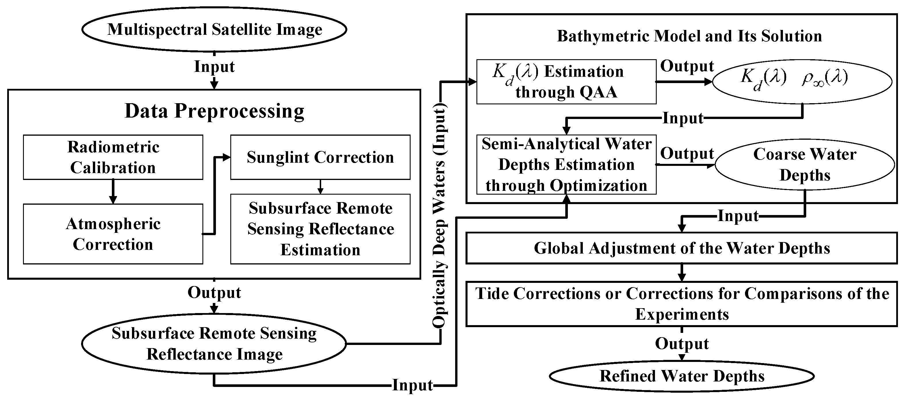
Figure 5.
The experimental multispectral images: (a) the ZY-3 multispectral image; and (b) the WV-3 multispectral image. Based on the division represented by the straight line, the western region of the WV-3 image may be seriously influenced by clouds; therefore, we only study the eastern region of the WV-3 image in our experiments.
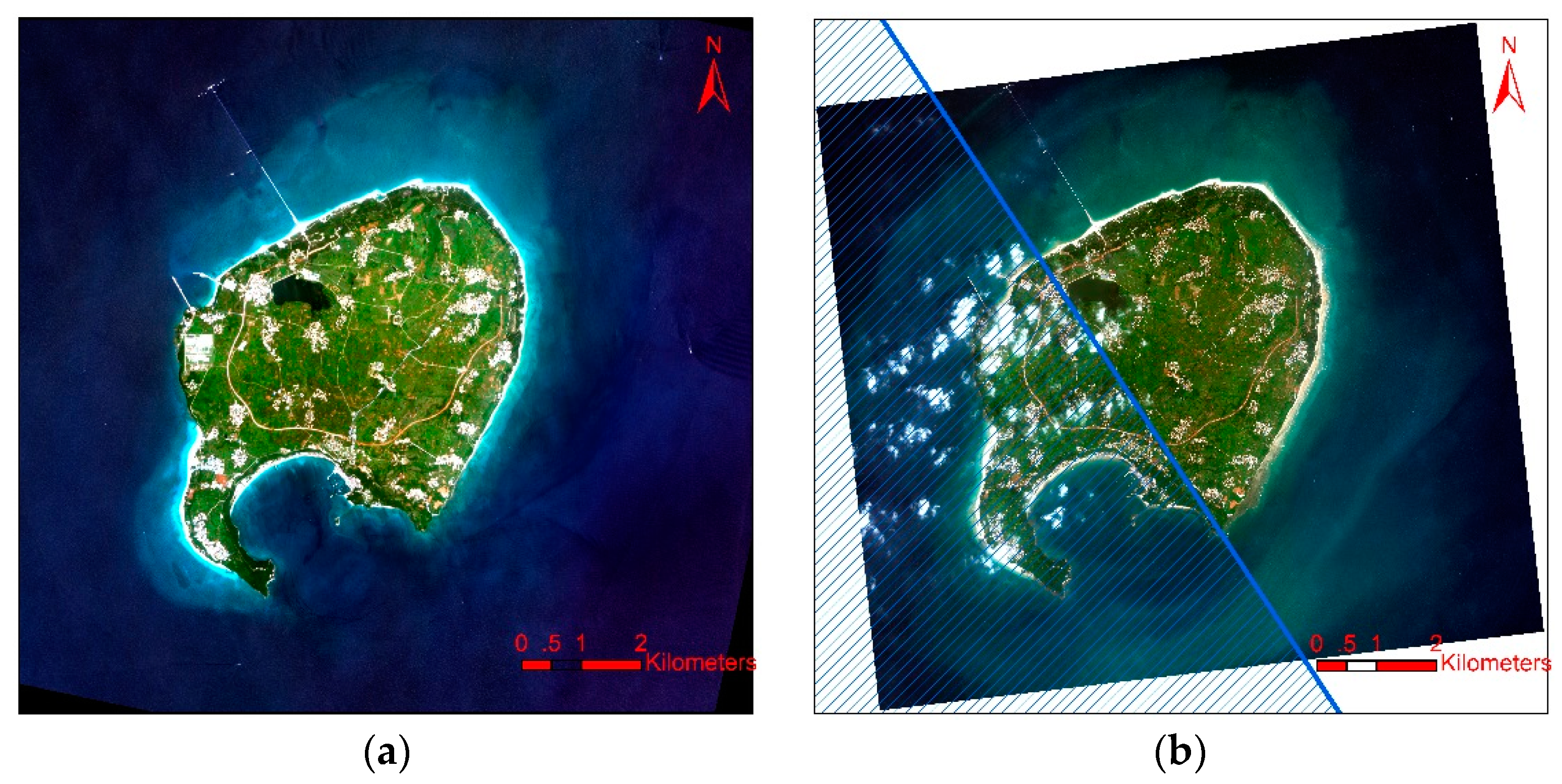
Figure 6.
The position distribution of the measured water depths: the red triangles are the stations where the water depths were measured, these measured water depths are used as water depth check points for the accuracy assessment.
Figure 6.
The position distribution of the measured water depths: the red triangles are the stations where the water depths were measured, these measured water depths are used as water depth check points for the accuracy assessment.

Figure 7.
The atmospheric correction approach.

Figure 8.
The two parts of the updated semi-analytic model.

Figure 9.
The water depths estimated by the ZY-3 image: (Top) before the global adjustment; and (Bottom) after the global adjustment.
Figure 9.
The water depths estimated by the ZY-3 image: (Top) before the global adjustment; and (Bottom) after the global adjustment.

Figure 10.
The water depths estimated by the WV-3 image: (Top) before the global adjustment; and (Bottom) after the global adjustment.
Figure 10.
The water depths estimated by the WV-3 image: (Top) before the global adjustment; and (Bottom) after the global adjustment.
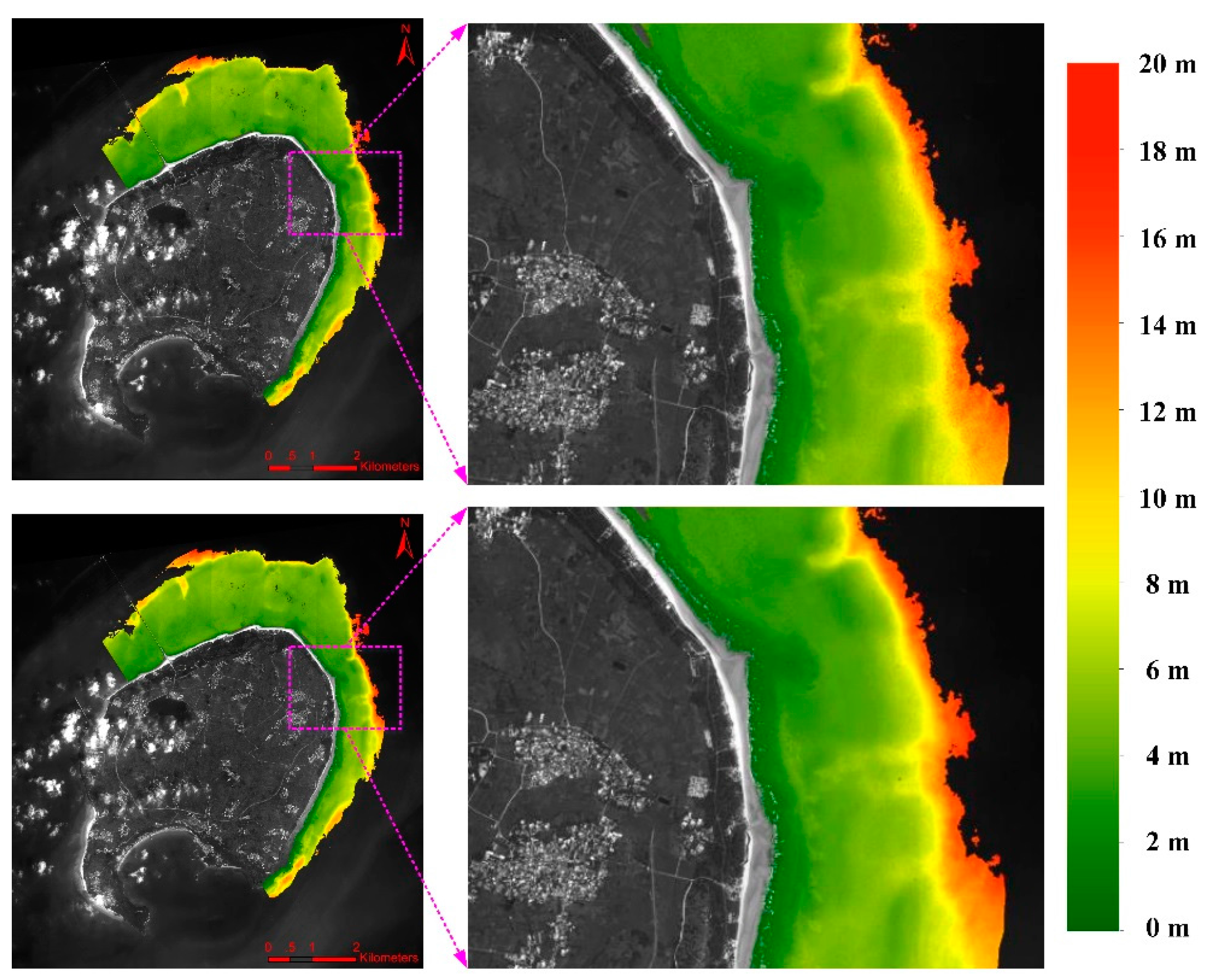
Figure 11.
The comparisons between the estimated and measured water depths: (a) ZY-3; and (b) WV-3.

Figure 12.
The Comparisons between the water depths estimated from the ZY-3 and the WV-3 images.
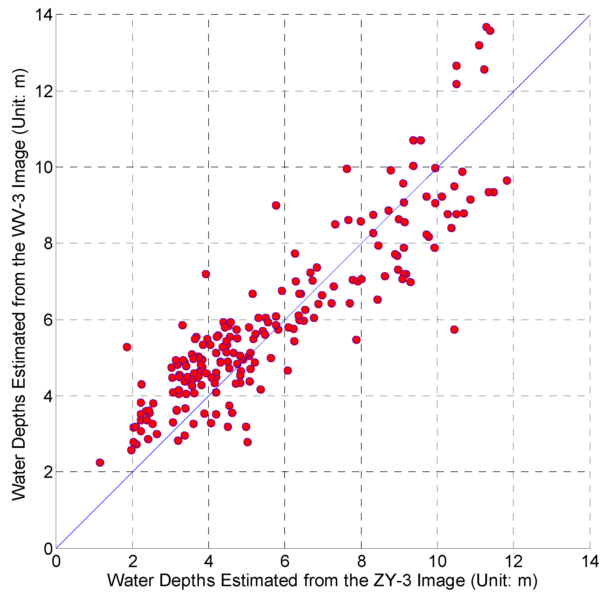
Figure 13.
The water depths along a transect of the two images: the dotted boxes mark some possible large outliers of the water depths of the ZY-3 or the WV-3 image before the global adjustment; the dotted circle marks the place where the local variations and the differences of the water depths estimated from the two images become large.

Table 1.
Band information of the ZY-3 multispectral satellite image.
| Bands | Wavelength (nm) | Radiometric Calibration Coefficients () | |
|---|---|---|---|
| Gain | Offset | ||
| Blue | 450–520 | 0.233 | 0 |
| Green | 520–590 | 0.2162 | 0 |
| Red | 630–690 | 0.1789 | 0 |
| Near-Infrared | 770–890 | 0.1949 | 0 |
Table 2.
Statistics of the Diffuse Attenuation Coefficients (WV-3).
| Bands | Coastal | Blue | Green | Yellow | Red | RedEdge |
|---|---|---|---|---|---|---|
| Mean | 0.0482 | 0.0529 | 0.0714 | 0.2776 | 0.4289 | 1.3665 |
| Std. Deviation | 0.00248 | 0.00201 | 0.00112 | 0.00091 | 0.00150 | 0.00073 |
| Skewness | 0.209 | 0.296 | 0.373 | 0.390 | 0.426 | 0.358 |
| Kurtosis 1 | 0.006 | 0.669 | 0.069 | −0.025 | 0.432 | −0.265 |
1 The Kurtosis has already been reduced by 3.
Table 3.
Statistics of the Diffuse Attenuation Coefficients (ZY-3).
| Bands | Blue | Green | Red |
|---|---|---|---|
| Mean | 0.0371 | 0.0677 | 0.4143 |
| Std. Deviation | 0.00947 | 0.00329 | 0.00265 |
| Skewness | −0.111 | 0.481 | 0.784 |
| Kurtosis 1 | 0.446 | −0.050 | 0.088 |
1 The kurtosis has already been reduced by 3.
Table 4.
Statistics of the differences between the estimated and measured water depths 1 (Unit: m)
| Satellite | Before Global Adjustment | After Global Adjustment | ||||
|---|---|---|---|---|---|---|
| MAX | MAE | RMSE | MAX | MAE | RMSE | |
| ZY-3 | 2.587 | 0.97 | 1.22 | 2.265 | 0.81 | 1.01 |
| WV-3 | 2.11 | 0.58 | 0.75 | 2.27 | 0.56 | 0.77 |
1 Note: MAX represents the maximum value of the absolute errors between the estimated and measured water depths, MAE represents the mean value of the absolute errors, and RMSE represents the root mean square error, which is calculated using the following equation:
where is the measured water depth and is the water depth estimated using the proposed approach.
Table 5.
Comparisons of the RMSEs obtained using different methods.
| Author/Method | Location | Data | RMSE (Unit: m) |
|---|---|---|---|
| Hu et al. (2014) | Pratas Atoll | Landsat ETM+ | 1.6 |
| North Danger Reefs | Landsat ETM+ | 1.1 | |
| Eugenio et al. (2015) | Granadilla area of Tenerife Island | WV-2 | 1.20 |
| Corralejo area of Fuerteventura Island | WV-2 | 1.94 | |
| Our Approach | Weizhou Island | ZY-3 | 1.01 |
| Weizhou Island | WV-3 | 0.77 |
© 2017 by the authors. Licensee MDPI, Basel, Switzerland. This article is an open access article distributed under the terms and conditions of the Creative Commons Attribution (CC BY) license (http://creativecommons.org/licenses/by/4.0/).
Share and Cite
MDPI and ACS Style
Huang, R.; Yu, K.; Wang, Y.; Wang, J.; Mu, L.; Wang, W. Bathymetry of the Coral Reefs of Weizhou Island Based on Multispectral Satellite Images. Remote Sens. 2017, 9, 750. https://doi.org/10.3390/rs9070750
AMA Style
Huang R, Yu K, Wang Y, Wang J, Mu L, Wang W. Bathymetry of the Coral Reefs of Weizhou Island Based on Multispectral Satellite Images. Remote Sensing. 2017; 9(7):750. https://doi.org/10.3390/rs9070750
Chicago/Turabian StyleHuang, Rongyong, Kefu Yu, Yinghui Wang, Jikun Wang, Lin Mu, and Wenhuan Wang. 2017. "Bathymetry of the Coral Reefs of Weizhou Island Based on Multispectral Satellite Images" Remote Sensing 9, no. 7: 750. https://doi.org/10.3390/rs9070750
Note that from the first issue of 2016, this journal uses article numbers instead of page numbers. See further details here.