
A Novel Method to Reconstruct Overhead High-Voltage Power Lines Using Cable Inspection Robot LiDAR Data


1
Department of Power and Mechanical Engineering, Wuhan University, Wuhan 430072, China
2
Guangdong Keystar Intelligent Robot Co., Ltd., Foshan 528000, China
3
Key Laboratory of Hydraulic Machinery Transients, Ministry of Education, Wuhan University, Wuhan 430072, China
*
Author to whom correspondence should be addressed.
Remote Sens. 2017, 9(7), 753; https://doi.org/10.3390/rs9070753
Submission received: 24 June 2017
/
Revised: 16 July 2017
/
Accepted: 17 July 2017
/
Published: 22 July 2017
Abstract
:Overhead high-voltage power lines are key components of power transmission and their monitoring has a very significant influence on security and reliability of power system. Advanced laser scanning techniques have been widely used to capture three-dimensional (3D) point clouds of power system scenes. Nevertheless, power line corridors are found in increasingly complex environments (e.g., mountains and forests), and the multi-loop structure on the same power line tower raises great challenges to process light detection and ranging (LiDAR) data. This paper addresses these challenges by constructing a new collection mode of LiDAR data for power lines using cable inspection robot (CIR). A novel method is proposed to extract and reconstruct power line using CIR LiDAR data, which has two advantages: (1) rapidly extracts power line point by position and orientation system (POS) extraction model; and (2) better solves pseudo-line during reconstruction of power line by structured partition. The proposed method mainly includes four steps: CIR LiDAR data generation, POS-based crude extraction, voxel-based accurate extraction and power line reconstruction. The feasibility and validity of the proposed method are verified by test site experiment and actual line experiment, demonstrating a fast and reliable solution to accurately reconstruct power line.
1. Introduction
High-voltage power lines are key components of the power transmission infrastructure to compensate for the long transmission distances and to reduce electricity transmission losses [1]. Globally, high-voltage power lines will increase from 5.5 million km in 2014 to 6.8 million km in 2020. In China, high-voltage power lines will grow 0.44 million km, with a global growth of 48% [2]. With the rapid growth of transmission network, power lines will inevitably cover more complex terrains, e.g., mountains, lakes or forests [3]. Power lines exposed long-termly in these harsh conditions (e.g., large temperature difference, high humidity, and vegetation encroachment [4,5]) might aggravate mechanical tension and electrical flashover, even leading to large area blackout, causing heavy national economic losses [6,7]. Therefore, this is urgent demand for monitoring power lines conveniently, rapidly and accurately to guarantee safe operation of transmission network [8].
With the development of detecting technology, LiDAR system is a good way to solve problems such as spatial orientation and continuous measurement, quickly obtaining high precision spatial information of transmission corridors [9,10]. Power line model can be obtained by extracting and reconstructing power line point cloud in 3D scene dataset, which can be used to achieve essential work, including monitoring the clearance between trees and power lines to identify and predicting dangers from vegetation [11]; providing professional electricity analysis to conduct power network design and upgrading; and supporting electric circuit management and decision-making. Therefore, power line extraction and reconstruction greatly improve intelligent level and efficiency of power line monitoring [12,13]. LiDAR system will play a more important role in the smart grid with decreasing cost of scanning laser.
At present, power line inspection with LiDAR mainly includes two methods: airborne laser scanning (ALS) and mobile laser scanning (MLS) [14,15]. ALS has achieved successful application on mobile measurement in power grid system. It has been accepted widely by power sector as the principle tool to monitor power line. The ALS-based methods have a set of process from raw point cloud to risk spot diagnosis. There are fruitful achievements on improving the precision and efficiency of power line reconstruction [16,17]. MLS, an emerging mobile mapping system, can obtain surface features rapidly by vehicles. Some experiments indicated that MLS can be used to inspect power lines because power lines are often distributed along the roads [18,19]. Taken together, the two methods have their advantages and disadvantages. ALS can collect rapidly and efficiently large-scale spatial data, but its point cloud is sparser. When the same airborne LiDAR system acquires data in a fixed gesture, the point distance will be greater with increased height and vice versa [20]. To obtain sufficient power line points, a helicopter has a relatively low flying height, which makes the working environment of helicopter complicated and dangerous. For MLS, it can obtain higher density point cloud and the average point distance of power lines can reach the centimeter-level, but it cannot pass over lakes or forests in a limited inspection area. Therefore, MLS is more suitable for monitoring power lines along the road in urban [21]. In recent years, a new LiDAR system, Geiger Mode (GM) LiDAR [22], is developed for commercial use. GM LiDAR requires much less power since the receiver is photon sensitive, producing high-resolution data with dramatically increased efficiency.
During the last few decades, many research works on the detection and reconstruction of power lines using air/vehicle-borne LiDAR have been reported [23,24]. Axelsson [25] presented a classification method of power lines by searching parallel and linear 2D structures based on Hough transform (HT) method. Melzer and Briese [26] proposed a method for power line extraction and modeling based on a bottom-up strategy and applied the iterative HT to identify single power line. McLaughlin [27] proposed a knowledge-based classification method for distinguishing power lines from their surroundings. Jwa and Sohn [28,29] introduced a voxel-based piecewise line detector (VPLD) method for automatically reconstructing power line. Liu et al. [30] detected power lines with a 2D gray-level image and introduced an improved HT. Kim and Sohn [31] used the random sample consensus (RANSAC) method and principal component analysis in feature extraction, as well as random forests as a classification technique. Sohn et al. [32] proposed a Markov random field (MRF) classifier, delineating the spatial context of linear and planar features, and reconstructed power line based on the location of the pylon with catenary model. Kim and Sohn [33] introduced a point-based supervised random forest method to classify five utility corridor objects from ALS. Based on this literature review, the existing methods to reconstruct power line can be roughly classified into four categories: HT method, statistical method, similar region growth method and connected component method. These methods have their characteristics and limitations in practice. For example, HT method extracts power line by the linear characteristics of the power line projected to the horizontal plane, which references some mature product of 2D image processing. However, it is difficult to identify power lines in the vertical, mixed or staggered layouts. The statistical method based on the elevation histogram is quicker and more efficient but may fail to separate power lines due to big sag or rugged terrain.
The multi-loop structure on the same tower is an efficient way to save land occupation for transmission corridors. However, the distribution of power lines is increasingly complex, with different layers and the increasing use of multi-loops. Power lines projected to the horizontal plane may be overlapping together, resulting in more difficulties in extracting single power line from areas of dense mixed objects using 2D image processing. Moreover, power line corridors cover growing areas, especially undulating terrains (e.g., mountains and forests), which raises great challenges to process LiDAR data by the statistical method based on the elevation histogram. Finally, an obvious difficulty of power line scanning of ALS/MLS is power lines are thin and long, thus ending up with a low density of points when the laser scanner is not close enough. This paper addresses these challenges by proposing a novel method to extract and reconstruct power line automatically and efficiently using CIR LiDAR. The method using CIR LiDAR is a good supplement for ALS/MLS to inspect transmission corridors in some complex environments.
This paper is organized as follows. Section 2 describes the mechanical structure of CIR and working principle of CIR LiDAR system. Section 3 presents the detailed method of extracting and reconstructing power line using CIR LiDAR data. Section 4 illustrates two experiments to verify the effectiveness and feasibility of the proposed method. Section 5 provides the corresponding discussions. Conclusions are summarized in Section 6.
2. CIR LiDAR System
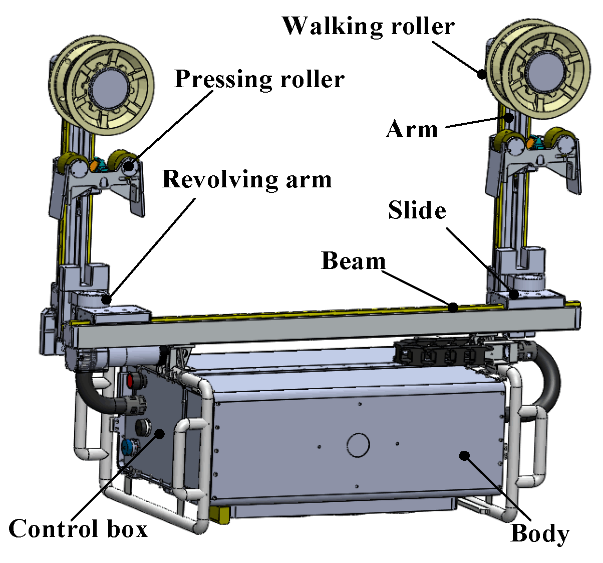
CIR LiDAR system integrated in CIR includes CIR self-positioning system and LiDAR system. The mechanical structure of the CIR is shown in Figure 1. CIR has two arms suspended on the traveling ground wire, and each arm consists of a walking joint, a pressing joint and a rotating joint. The walking joints provide driving force for robot. The compression joints allow the robot to adapt different line angles. The two arms alternately loosen the pressing rollers using peristaltic way across obstacles. CIR weighs less than 50 kg without carrying inspection equipment and has an average speed of 3–4 km per hour. The self-developed CIR has completed demonstration applications in the state grid.
CIR is hung on the ground wire as its moving path to collect data points by CIR LiDAR system as illustrated in Figure 2. The starting tower and the ending tower, respectively, have installed a set of automatic up/down-line devices to replace manual hoisting onto the ground wire, and solar charging stations are installed on some towers to supply power for CIR.
CIR self-positioning system is used to obtain its position and orientation in real time, which mainly includes two parts: inspection database and positioning sensors. The inspection database stores construction specifications of power lines as prior data, while positioning sensors include wheeled odometer, obliquity sensor and visual odometer, assisting LiDAR system to achieve precise positioning in some extreme cases, such as electromagnetic interference, signal blocking, etc.
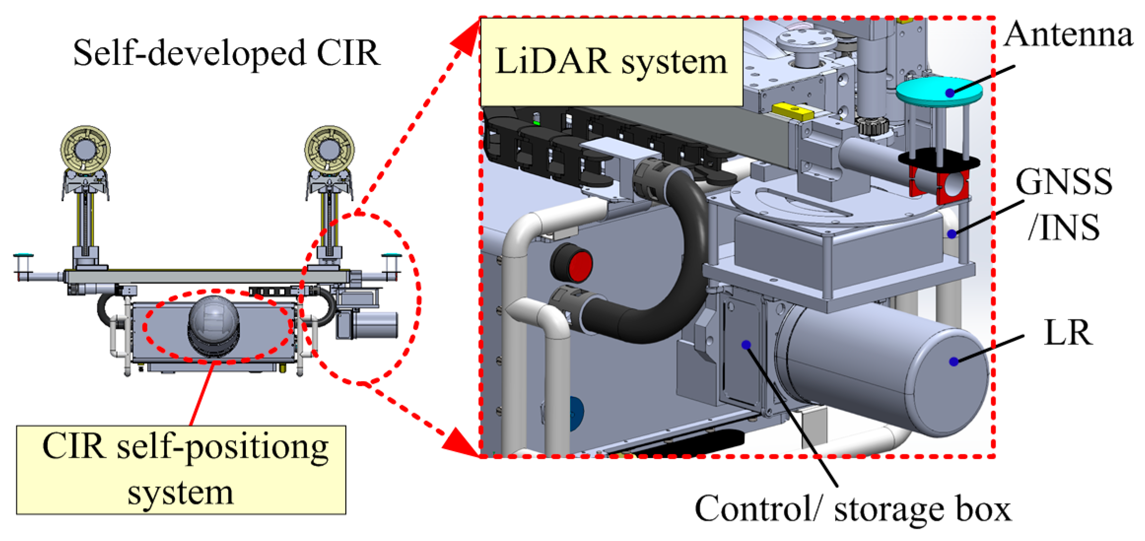
LiDAR system includes scanning laser radar (LR) and combined navigation consisting of global navigation satellite system (GNSS) and inertial navigation system (INS). LR can measure the distances between sensors and target points. The 3D precise location of the scanner is obtained by GNSS in the spatial domain. INS is used to measure the posture parameters of the scanner such as roll angle, pitch angle and yaw angle. The working principle of LiDAR system is shown in Figure 3. The position of target point is resolved by coordinate transformation in the three coordinate systems. The first one is the instantaneous laser coordinate system (LCS) with center of laser as its origin. The second one is the body frame system (BFS) with the origin of three sensitive axis of INS as its origin. The third one is the geodetic coordinate system (GCS) with the center of the earth as its origin, usually using WGS-84. As a result, the precise 3D coordinates of laser spot can be resolved by time synchronization, interpolation algorithm, coordinate system transformation, etc.
The key components of CIR LiDAR system are shown in Figure 4. CIR moves along ground wire to perform inspection mission. Towers, power lines and trees are usually lower than CIR’s position. Thus, LR and GNSS/INS are installed on the end of CIR’s body. Moreover, their dimensions and weights are also strictly controlled using 3D dynamic simulation to ensure the feasible operations. Two antennas of GNSS are installed on both ends of the beam to avoid motion interference during crossing obstacles. The beam of CIR has high strength and rigidity, preventing strong wobble to ensure relative positions of LR, GNSS/INS, and antenna.
3. Methods
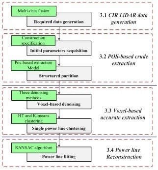
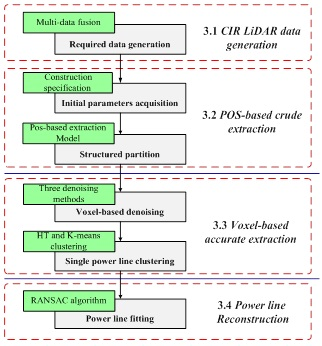
We propose a new method to extract and reconstruct power line as illustrated in Figure 5, which mainly includes four steps: CIR LiDAR data generation, POS-based crude extraction, voxel-based accurate extraction and power line reconstruction.
3.1. CIR LiDAR Data Generation
3.1.1. Data Characteristic
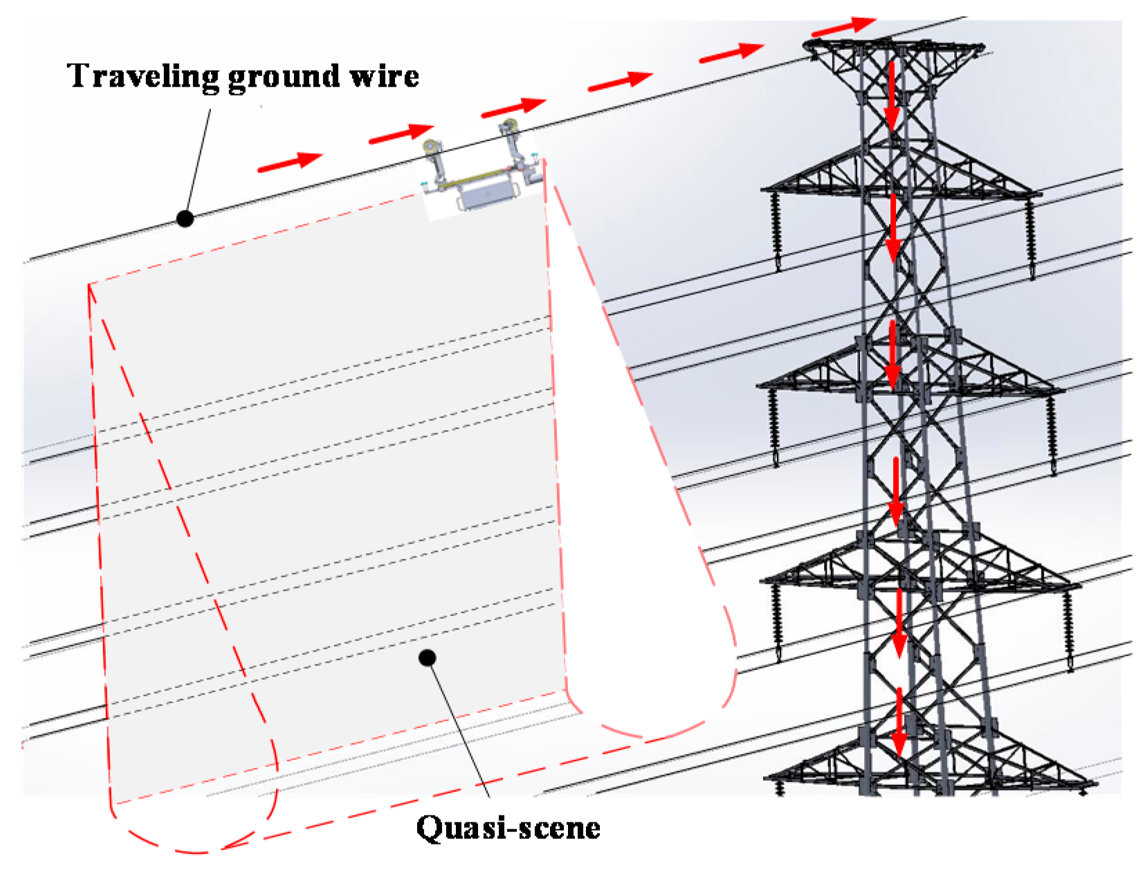
CIR LiDAR system, a multi-source integration system, can provide three kinds of data: prior data, high-precision POS data and 3D scene data. Prior data derived from construction specifications of towers are stored in the inspection database. The construction specifications of towers form some characteristics of power line dataset: power lines in different layers have fixed spacing; power lines in a span segment projected to the horizontal plane are parallel straight lines; and power lines belong to natural suspension lines in accordance with hyperbolic cosine equation. High-precision POS data can represent orientation and shape of all power lines in a span segment because CIR moves along the ground wire. The 3D scene data are huge and dense, owing to moving at low speed. Some detailed objects on power line, such as fittings, are also contained in the 3D scene data. Besides, the ground wire data are not included in 3D scene point cloud, which is a quasi-scene point cloud, as illustrated in Figure 6, mainly because of the nearest scanning distance of LR (>1 m in this paper) and installation position below the GNSS/INS (as seen in Figure 4).
3.1.2. Data Generation
CIR LiDAR system includes three subsystems: CIR self-positioning system, combined navigation system and laser radar system. Various raw data collected by the three subsystems should be fully fused to generate the four required data to achieve the subsequent power line extraction and reconstruction. The flow chart of CIR LiDAR data generation is shown in Figure 7.
Inspection database has been stored in CIR self-positioning system before inspection tasks. The prior data, i.e., tower construction data and tower reference point, can be obtained by database retrieval in the inspection database.
Positioning sensors in CIR self-positioning system assist combined navigation system to achieve high-precision POS data in some extreme cases, such as signal blocking, etc. In positioning sensors, wheeled odometer is modified by obliquity sensor when over-obstacle, acceleration or deceleration. Visual odometer is used to improve positioning accuracy as walking rollers of CIR are in slippery or jolty conditions. In combined navigation, INS fuses with positioning sensors by loose coupling to obtain relative positioning data. GNSS can get absolute positioning data by satellite. Absolute positioning data constantly modify drift errors of relative positioning data. Both of the above data are processed through extended Kalman filtering to achieve high-precision POS data. Then, traveling ground wire data can be generated by compensating the offset from the structural parameter of CIR.
Laser radar system can generate 3D scene point clouds. The raw radar data collected by transmitter and receiver need to be preprocessed as the walking velocity of CIR is slow and the amount of laser footprints is huge. Then, the high precision POS data and laser footprints are associated together by geographical matching to generate quasi-scene point clouds of transmission corridors.
3.2. POS-Based Crude Extraction
3.2.1. Prior Data Acquisition
A typical double-loop two-bundle power line is taken as an example to illustrate prior data acquisition according to tower construction specification. The distribution of double-loop two-bundle power line is shown in Figure 8.
All conductors are divided into two loops according to the center line of the tower. The three-phase conductors on the left are I-loop, and the three-phase conductors on the right are II-loop. CIR walks on ground wire one of left side. The ground wire as a reference line is used to identify all power lines in the Steps 1–3. The specific procedures are listed as follows.
Step 1: Construct and . Ground wire partition matrix represents type of ground wire, which is defined as:
where represents the traveling ground wire, and represents the other ground wire.
Phase-conductor partition matrix represents distribution of phase-conductor. is expressed as follows:
where , , and represent three-phase conductors of I-loop; and , , and represent three-phase conductors of II-loop. Each element of includes two sub-conductors because each phase conductor is two-bundle conductor.
Step 2: Construct the tower construction matrix , which represents the distances between all kinds of power lines in a span segment in the Z-direction. is defined as:
Step 3: Determine , which represents the distance between traveling ground wire and central axis of tower.
3.2.2. Structured Partition
Typical power line reconstruction is based on the down-top decomposition of the raw point cloud. The ground points are filtered out first, and then power line points are identified according to the classification of characteristics. The filtering of LiDAR dataset is a fundamental step. Therefore, different filtering algorithms have been put forward, such as mathematical morphology filtering [34,35], slope filtering [36], and segmentation filtering [37]. The work group of ISPRS compared eight filtering algorithms [38], showing the undesired effects for steep slope or dense forest, which often occur in transmission corridors. Based on the characteristics of CIR LiDAR data, the POS-based structured partition is used to crudely extract power line. The advantages of POS-based structured partition have two aspects:
- Filtering out ground points based on the prior data and the POS data, without the filtering algorithm, solves the undesired effects for steep slope or dense forest.
- Defining a strategy from layer to partition according to the topology of power lines results in the better extraction efficiency.
The steps of the POS-based structured partition are shown as follows:
Step 1: Eliminate ground points using the elevation threshold, . Determine the span segment of power line according to the reference points of two adjacent towers. Get the elevation minimum, , of the high-precision POS data in the span segment. Thus, is described as
where is column element of tower construction matrix ; and d is the adjustment value. Therefore, points corresponding to Z-coordinate values less than the will be eliminated from the raw point cloud.
Step 2: Extract power line points in each layer. The quasi-scene point clouds are applied the WGS-84 coordinate system. The walking path of CIR is mainly composed of spans connected one by one, so the local engineering coordinate system is established as illustrated in Figure 9. Tower reference point mentioned in Section 3.2.1 can obtain the precise locations of the suspension points. In a span segment, the suspension point of litter-number tower P1 is considered as the origin of the engineering coordinate system (ECS) O’, and the elevation is applied as the z-axis of the ECS. The XYP presents the horizontal plane of the GCS. The two suspension points (P1 and P2) are projected to XYP, generating two points (P1’ and P2’, respectively). The Z’-axis (z-axis of ECS) is parallel to the Z-axis through point P1. The optimal coordinate plane (OCP) can be determined by lines P1’P2’ and P1P1’, which are perpendicular to XYP. In the OCP, line P1P2’’ is parallel to line P1’P2’ through point P1, intersecting line P2P2’ at point P2’’. Line P1P2’’ is defined as the y-axis of ECS as illustrated in Figure 9.
The raw point cloud datasets relative to GCS can be transformed to ECS by rotating z-axis and shifting the origin. The transformation matrix T is expressed as follows.
where .
(x,y,z) presents the coordinate of an arbitrary point in the GCS. is the coordinate of the suspension point P1 in the GCS, so the coordinate of an arbitrary point in the ECS () can be calculated in Equation (5).
The POS data present discrete distribution in the OCP. The model of the power line can be determined by fitting. Because the distance between the two towers is long and moment of any point is almost zero, the power line can be considered as an ideal soft cable. The power line model can be fulfilled according to the catenary equation. When the height difference of two suspension points is much smaller than the span value, nonlinear catenary equation can be simplified to linear polynomial according to the Lagrange polynomial. These points in the OCP are fitted to quadratic polynomial based on least square method. The curve model fitting POS data is obtained by Equation (7).
The point clouds of power line transformed the coordinate are projected to OCP. The point clouds of power lines in the same layer will be stacked together, forming discrete points in accordance with layer distribution. The spacing of each layer power line is prescribed in the tower construction specification. According to the spacings, each layer’s power line points can be extracted by the fitting POS-based model, as illustrated in Figure 10. The remaining surface points (e.g., phase spacers) and noise points (e.g., treetops) can be further removed.
However, when the robot is walking on the traveling ground wire, the power line is attached to additional sag due to the additional weight of the robot, as illustrated in Figure 11. Additional sag function can be expressed:
where is additional sag; S is the cross-sectional area of ground wire; W is the weight of CIR; L is the horizontal spacing; is horizontal stress of power line; and is the increase coefficient of the impact effect. The impact effect results from the vibrations generated by the walking of CIR and wind. To separate perfectly each layer’s power line points of overhead multi-loop power lines, the fitting POS-based model is revised with the additional sag function, as shown in Equation (9).
Step 3: Subtract prior data mentioned in Section 3.2.1 from the y-coordinate values of each layer’s power line points. The power line with a positive sign of the y-coordinate values is identified as the layer’s CIR side power line point. On the contrary, the power line with a negative sign of the y-coordinate values is identified as the layer’s non-CIR side power line point.
3.3. Voxel-Based Accurate Extraction
3.3.1. Voxel-Based Denoising
There are still many noise points in the structured partition point clouds. For example, the residual of high vegetation and fittings will also generate noise points. The CIR LiDAR data are real 3D point datasets. Voxel-based methods are widely used to eliminate noise points because they make full use of 3D structural features. Therefore, we also adopt the voxel-based methods for denoising in the partitions as shown in Figure 12.
The voxelization is a fundamental work. Each point in the partitions should be associated with a voxel by grid coordinate system. The minimum coordinate (xmin, ymin, zmin) in each partition dataset is set as (x0, y0, z0). Δx = Δy = Δz is set as grid size, which should be less than the minimum distance of bundled conductors. The location of the corresponding voxel is calculated by the coordinate of the point in the partitions as follows
where: i, j and k are column, row and layer of the scanning point in 3D voxel grid, respectively.
The steps from eliminating three kinds of noise are shown as follows:
Step 1: Remove the nonlinear characteristic noise in the partition. Partition dataset can be classified according to the features of geometry and direction. Eigenvector decomposition is conducted by the 3D coordinates of the points in the voxels. Three eigenvalues are obtained: λ1, λ2, and λ3 (λ1 ≥ λ2 ≥ λ3 ≥ 0). The distributions of different target eigenvalues have obvious differences, determining the spatial distribution of the local point cloud. The relationships among these three eigenvalues indicate the distributions of the 3D points: if λ1 >> λ2 ≈ λ3, the points are linear distribution; if λ1 ≈ λ2 >> λ3, the points are planar distribution; and if λ1 ≈ λ2 ≈ λ3 [39,40]. Thus, power line, vegetation and building can be classified by the dimension characteristics of eigenvalues.
Based on this principle, Equation (11) helps to detect linear similar structures, while the linearity of eigenvalues also shows high values at building edges as well as power line.
If the linearity is greater than a threshold value (0.38), the voxel is retained; otherwise, it is eliminated. Thus, residual vegetation and buildings can be separated.
Step 2: Remove the linear noise in vertical direction. Point cloud includes a limited number of power line point, tower point, interval rods and other fittings point after crude extract partition in Section 3.2, which is extracted together because of linear characteristic. Vertical continuity parameter is defined to eliminate these point cloud; the vertical continuity of power line point is far lower than the tower and spacer point. Therefore, the vertical continuity is calculated for each voxel and if the value is less than a threshold value (3), it is retained; otherwise, it is eliminated. Through structured partition in Section 3.1, there are only close bundled conductors left within each partition’s power line point. Thus, the threshold should be smaller than the spacing between bundled conductors.
Step 3: Remove residual discrete noise in the partition. There are still some sparse noise points to be eliminated by density distribution of point cloud using the statistical method [41].
- Calculate the point density of voxels Dvoxel with respect to each single voxel and obtain the density interval [Dmin, Dmax] based on the maximum and minimum values of the point density. Set the minimum interval size as Ds. The range can be divided into n levels. Then, get the set S = {Sj, j = 1, 2, …, n}, where n = int((Dmax − Dmin)/Ds).
- If k = int((Dvoxel−Dmin)/Ds) equal to a certain interval value Sj, then increase the accumulation value Accj by 1, i.e., Accj = Accj + 1, to get the point density accumulation curve of Dvoxel and Acc. From the curve, the peak interval corresponds to the non-power line points and the others correspond to power line points.
- Calculate the partial derivative and find the peak interval based on the point density accumulation curve. Eliminate the points inside the grids corresponding to the peak interval and the remained points are power line points.
3.3.2. Single Power Line Clustering
There is only ordered point cloud of bundled conductor after the above-process for each structured partition. Its linear feature is obvious, and the number of power lines in this region is certain according to the prior data. Thus, single power line points can be extracted using HT and K-means algorithm. Single power line can be extracted using edge detection and linear detection, as shown in Figure 13.
Point clouds of power lines are projected to the XY-plane by the above structured partition and denoising, generating grids by the scope of the area. According to the width (W) of the input image and the range of projection datasets in the X-axis, the sampling interval (inv) is calculated using Equation (12).
The range of projection datasets in the Y-axis and the sampling interval (inv) can be used to calculate the height of elevation image (H) as follows.
The coordinates of partition power line points in the GCS can be converted to row number (row) and column number (col) of the corresponding grid.
Then the projected datasets are conducted resampling. The elevation of each point is standardized. If a grid has several data points, the largest elevation of these points will be normalized. The standardized elevation is converted to the pixel gray value (gray) in Equation (15).
where is the range of gray.
Canny operator is used to extract the edge for elevation image, and then Hough detection method is used to extract straight line. The power point cloud by the projection plane is roughly uniform discrete points both sides of power line, so the similar slope and concentrated distribution straight lines will be detected in certain intervals. Processing method is as follows:
- Link together straight line segments in the same direction, judge on connectivity according to the endpoint distance of two adjacent straight line segments.
- Delete the short line segments of the unlinked short line segments.
- Execute clustering analysis for the rest of the straight line segments in Hough space. The K-means clustering algorithm is improved by the prior data: select k random data points in Hough space to represent the initial clustering center, k is the number of the bundled conductors; assign each point in the Hough space to its nearest the center of the cluster, which makes the distance between the clustering as big as possible and the distance in clustering as small as possible.
After K-means clustering, straight lines detected in the elevation image are divided into k classes. Straight lines detected by Hough transform are classified. Set endpoints of the straight line as input data, carry out the linear least squares fitting, and extract vector data of power lines. Due to the prior data, the algorithm can generate real line number in accordance with point cloud projection lines.
After the above steps, straight lines of sub-wires in the XY-plane projection are obtained. According to the equation of center line, laser points of each power line are calculated: compute 2D distances from laser points to center line of power line in the XY-plane and judge if the point belongs to the power line; repeat the cycle until there are no points that meet the condition. Finally, laser points on every power line can be obtained.
3.4. Power Line Reconstruction
Single power line point cloud is to be fitted curves with the optimal catenary model. In order to simplify the operation, nonlinear catenary equation is simplified to linear polynomial according to the Lagrange polynomial principle. The coordinate system of power line model is established in Section 3.2.2: the suspension point O’ is set as the origin and OCP is set as the fitting plane.
The least square method is not suitable to fit single power line because the method tries to adapt to all the points including the outliers. Therefore, we use RANSAC algorithm to fit single power line. RANSAC algorithm evaluates repeatedly the estimated model by the distance from the inner points to the hypothetical model. Thus, the hypothetical model is very important, directly impacting on the final results. In the proposed method, the POS-based extraction model is used as the original hypothetical model, and the optimal model of single power line can be finally obtained using RANSAC algorithm.
4. Experiments and Results
4.1. Test Site Experiment
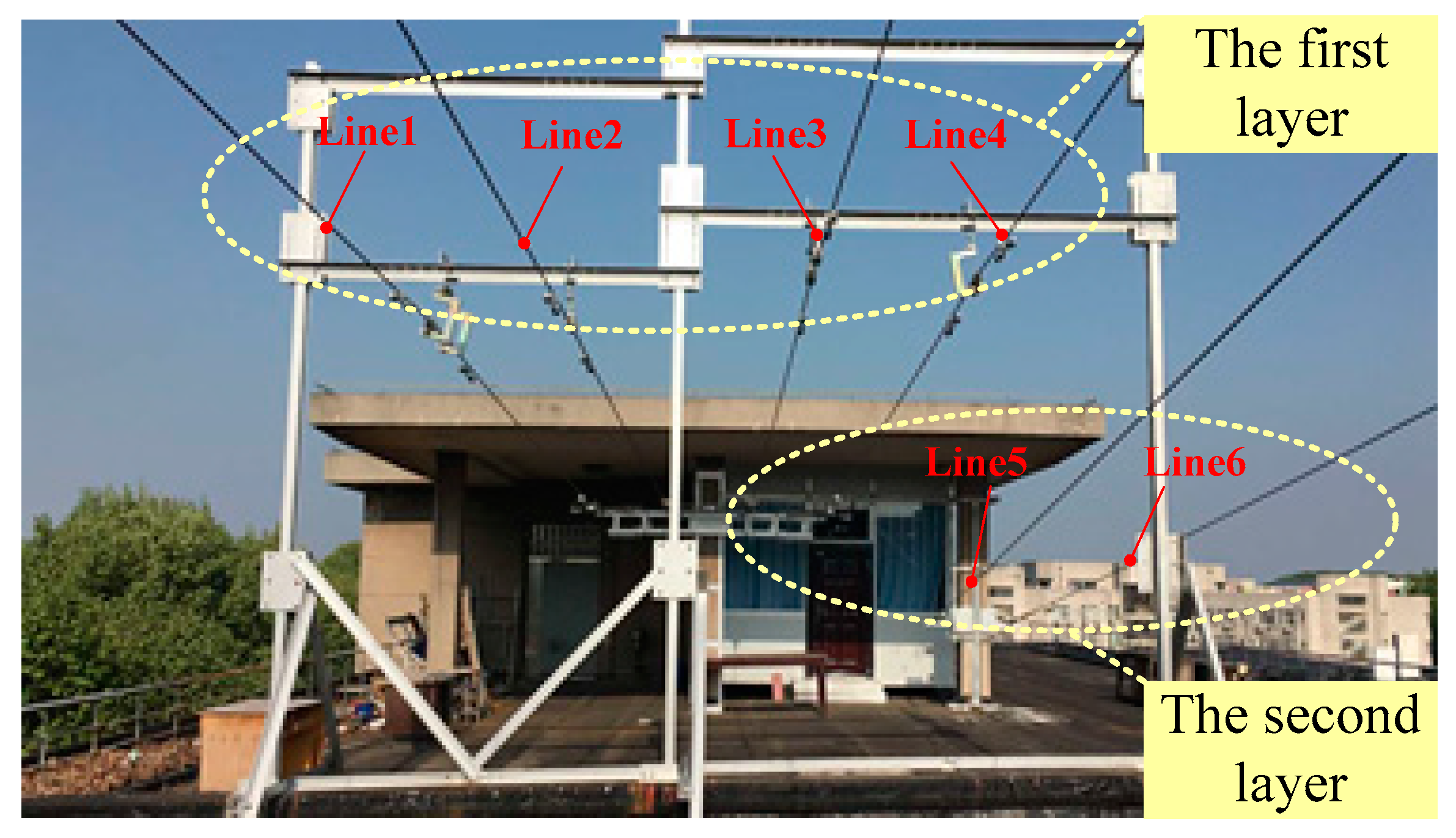
To validate the proposed method, the self-developed CIR with LiDAR system has carried out many experiments in a test site about 50 m in length and 30 m in width. The test site has six built up parallel power lines: Lines 1–4 on the first layer and Lines 5 and 6 on the second layer. There are tall trees and buildings around the test site. A photo of the test site is shown in Figure 14.
The test site is built up on the roof platform. There are no building or tree occlusions, creating a good condition for satellite signals. In addition, these power lines are unloaded high-voltage. Therefore, the POS data and point cloud dataset can be directly calculated without using positioning sensors in CIR self-positioning system. The distribution of these power lines is not strictly complied with the construction specification due to size limit of the test site. CIR moves along Line 6 because there are no automatic online/offline devices installed, and the test site experiment needs to adjust prior parameter acquisition according to the actual situation.
The quasi-scene point cloud of test site has 28,090,884 points, and the average point density is 7011 per square meter. It can be seen that the point cloud collected by the CIR LiDAR is denser. The elevation rendering of the raw point cloud is presented in Figure 15.
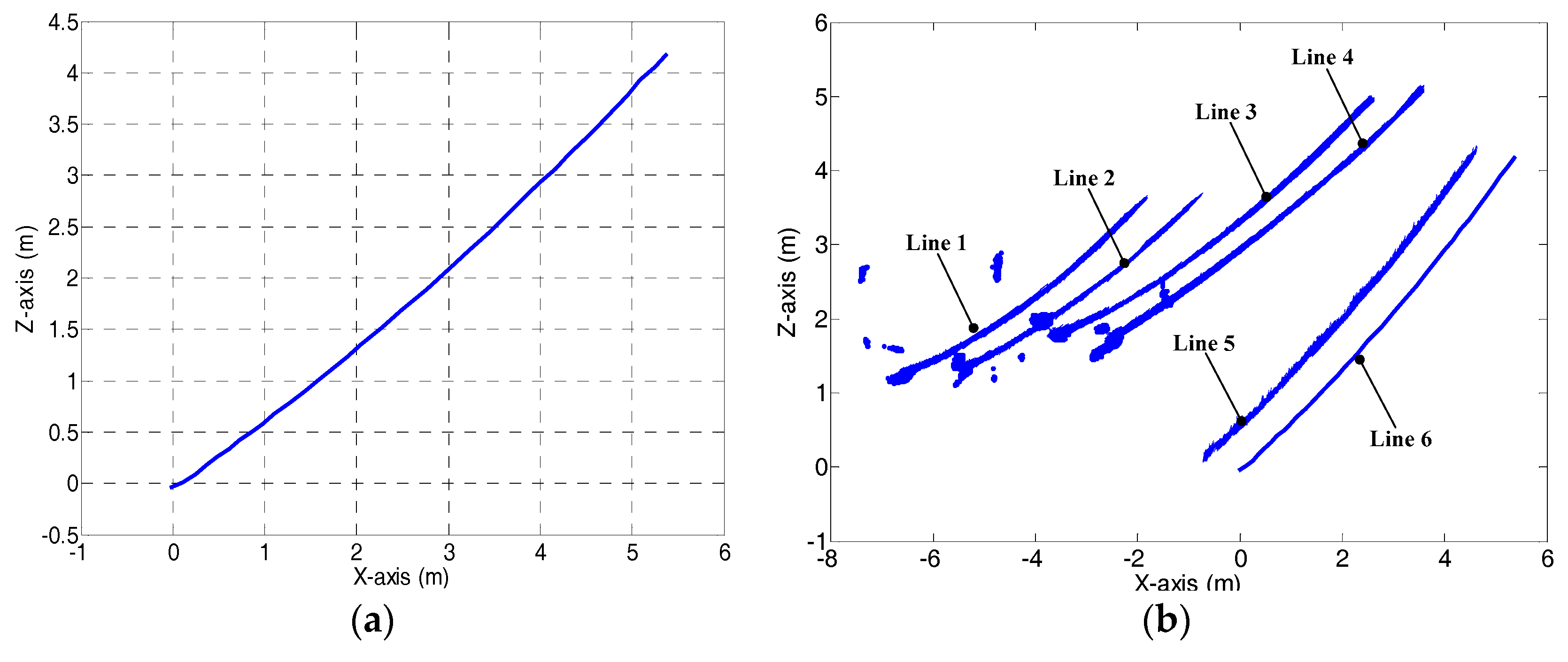
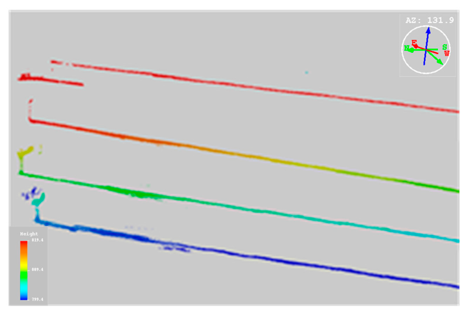
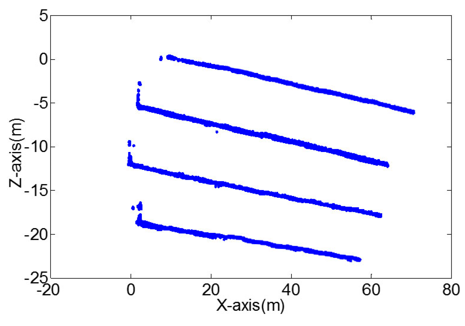
Ground points, and most vegetation and building points are eliminated from the quasi-scene point cloud of test site by POS-based crude extraction, as shown in Figure 16. The result of structured partition is shown in Figure 17. High-precision POS data are projected to the OCP, as shown in Figure 17a, and all power line point clouds are projected to the OCP in Figure 17b, which still has some noise points. Lines 1–6 are divided into three partitions (Lines 1 and 2, Lines 3 and 4, and Lines 5 and 6) by structured partition. There are two power lines in the each partition, which could reflect bundle conductor configuration of high-voltage transmission line.
Voxel-based accurate extraction can complete respectively the denoising and clustering for the three partitions. Figure 18 shows the process result of Lines 1 and 2 partition as an example. Finally, all power lines are fitted by RANSAC algorithm, as shown in Figure 19. The power lines are not fully parallel because the erection of test site does not strictly comply with the specification, which is consistent with practical situations.
4.2. Actual Line Experiment
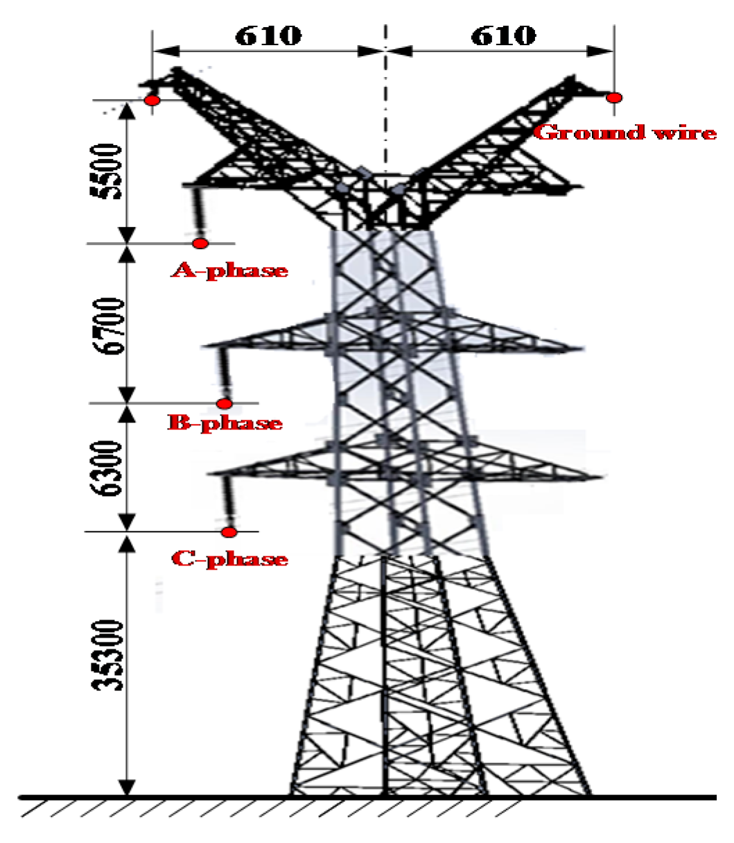
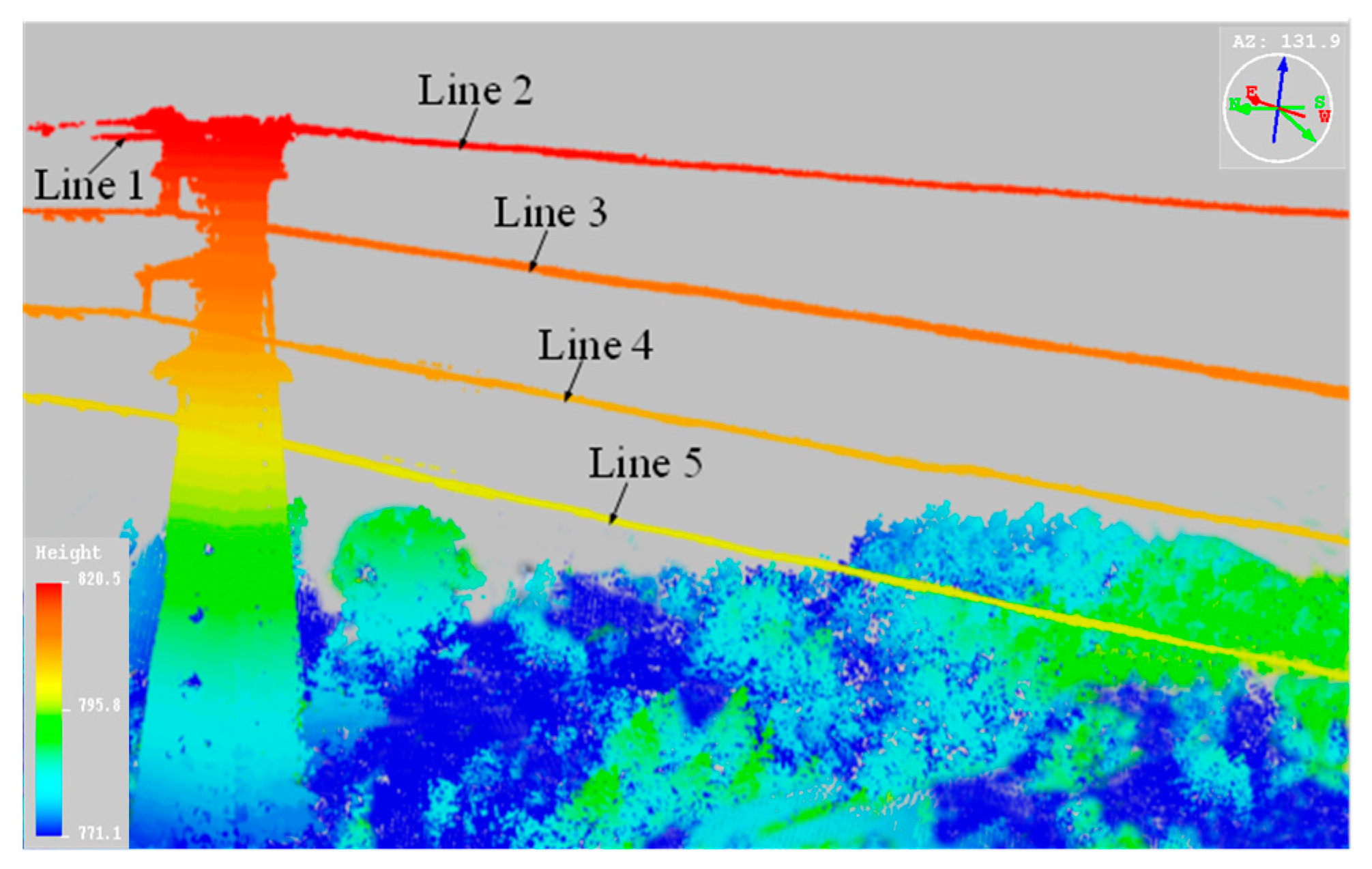
To verify the validity and feasibility of the proposed method, actual line experiment is conducted with CIR LiDAR system. The experimental site is located in the Changbai Mountains, Jilin Province, China, which has steep slope and dense forest. The actual lines are loaded 220 KV high voltages. Positioning sensors in CIR self-positioning system assist combined navigation system to achieve high-precision POS data and 3D scene point cloud. There are five power lines on the tower, as shown in Figure 20. The construction specification of actual line experiment is shown in Figure 21.
The tower has been installed a set of automatic up/down-line device. CIR moves along the left side of ground wire in a span segment, then climbs up and goes down the same tower. The quasi-scene point cloud of the actual line has 130,022,909 points, and the average point density is 15,650 per square meter. The elevation rendering of the raw point cloud is presented in Figure 22. Only a small portion of the traveling ground wire can be seen near the tower collected during up/down-tower process using up/down-line devices.
Figure 23 shows that all ground points, and most vegetation and tower points are eliminated from quasi-scene point cloud of the actual line. Some points of fittings, such as insulators closer to the suspension point, are extracted together. These points have distinctive feature with concentrated distribution. The processed power line points are projected to OCP, and there are still some noise points in Figure 24. Lines 2–5 are divided into four partitions.
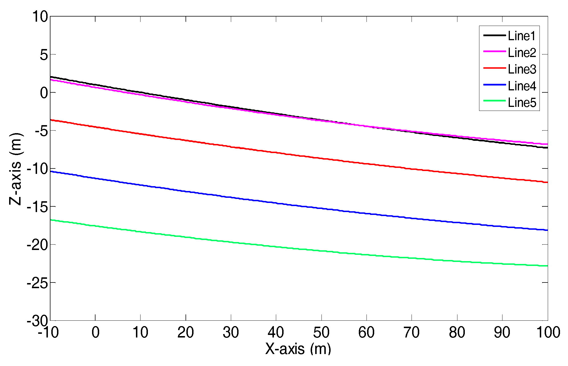
Because the actual power lines are not bundle conductor, voxel-based accurate extraction only needs to complete the partitions denoising. Finally, all of the power lines are fitted by RANSAC algorithm, and the power line models are shown in Figure 25. The power lines are parallel in fixed spacing and there is an overlap between Lines 1 and 2, which is consistent with the practical situation.
The results of extraction and fitting of each power line are listed in Table 1. For the five power lines, the mean extraction correctness reaches 95.7%, the mean extraction integrality reaches 87.6% and the mean fitting precision is less than 0.056. Line 1 is traveling ground wire collected by the POS of CIR LiDAR, and Lines 2–5 are collected by the LR. The point cloud of Line 1 is naturally separated from raw point cloud. Therefore, the extraction accuracy of Line 1 is 100% and fitting precision of Line 1 is also the highest. In the Lines 2–5, Line 2 is also ground wire, which is thinner than conductor wires. The number of Line 2 point cloud is less than Lines 3–5. Thus, the correctness and fitting precision of Line 2 are relatively poor, while the integrality of Line 2 is relatively good. Line 3 is closer to CIR in the three-phase conductors, thus has better extraction and fitting results.
5. Discussion
The proposed method was developed to solve two problems. First, CIR mode provides a useful supplement for popular ALS/MLS mode to capture 3D point clouds of power system scenes. Compared with ALS view from sky to ground, CIR LiDAR data can avoid the missing information of power line, which is thin and long, thus ending up with a low density of points when the laser scanner is not close enough. From two experimental data sets, we can see CIR LiDAR data are very dense—over three orders of magnitude greater than ALS. Different from dense-breakage-dense distribution pattern of MLS, CIR LiDAR data can also avoid blocking by trees or buildings. Power line points of CIR LiDAR dataset are sequential with the similar advantage to ALS. CIR LiDAR scanning is along ground wire, which completely focuses on the power line corridors. Thus, CIR mode can capture more detailed scenes (e.g., dampers and insulators) on power lines.
The second contribution of the proposed method, perhaps more important than the first, is that CIR moves along ground wire, forming particular characteristics other than non-contact mode of LiDAR data (i.e., ALS and MLS): robot traveling track, distributions of ground wires and power lines are closely related. For example, power lines are the highest objects in the local scope according to tower construction specification. Therefore, CIR LiDAR can quickly extract all power line points without filtering algorithms, which verifies that only constructing the elevation threshold can remove large amounts of non-powerline points to simplify the subsequent process in our two experiments. Power line point clouds with an apparent layer-parallel distribution projected to OCP, will overlap each other, leading to poor extraction effect using mature image algorithms, and the extraction effect would get worse with the growing loops. Therefore, it is very meaningful to classify power line points in a layer-by-layer way. However, model of power line is a catenary, which is difficult to completely classify by means of the elevation threshold. The extraction model of the proposed method combined the prior data and the POS data can be used to classify power line point clouds in layer-by-layer way.
There are still some limitations to the method. For example, a dual-antenna can effectively improve navigation deviation caused by low-speed straight line running for a long time. However, this approach requires enough baseline lengths, which is a challenge for CIR integration. In addition, because CIR moves along the ground wire, some complex environmental conditions have effect on ground wire morphology to influence CIR LIDAR data and the POS-based extraction model. CIR may wobble under the action of wind load, producing unwanted noise. There are all kinds of fittings installed on high-voltage transmission lines. During the over-obstacle motion, CIR needs to stop and repeatedly adjust its pose, causing a very large amount of redundant data. The above-mentioned situations would influence power line extraction and reconstruction.
6. Conclusions
In the study, we construct a novel collection mode of LiDAR data cloud using CIR, and propose an entire method to extract and reconstruct power line from raw point cloud. The main conclusions of our study are as follows:
- (1)
- The self-developed CIR has successfully completed an actual line trial, so CIR can become a new type of carrying platform to collect LiDAR data. This collection model using CIR is a good supplement for ALS and MLS to inspect transmission corridors in some complex environments (e.g., mountains and forests).
- (2)
- CIR LiDAR system can generate prior data, high-precision POS data and 3D scene data. Prior data and POS data are used to construct the POS-based extraction model to achieve structured partition. Structured partition can divide power line into some small partitions according to the topology of power lines, greatly enhancing correctness of voxel-based extraction and efficiency of reconstruction.
- (3)
- Test site experiment verifies that bundle conductors can be effectively extracted in small regions by structured partition method. Actual line experiment shows that the proposed method is feasible, with high extraction correctness over 95% and RMSE less than 0.077.
While the proposed method performs well overall, CIR LiDAR, a contact wire mode to capture 3D scene data, is still in initial development phase. In the future, more actual line tests will be carried out after the approval and permit by relevant power sectors to further improve and expand the method. This work mainly focuses on two aspects: (1) studying different types of transmission lines, especially multi-loop power lines; and (2) collecting CIR LiDAR data of multiple span segments to reconstruct power line corridors.
Supplementary Materials
Supplementary File 1Acknowledgments
This work is supported by Guangdong Robot Special Project (2015B090922007), Foshan Technical Innovation Team Project (2015IT100143), National Science and Technology Major Project (2014ZX04015021) and South Wisdom Valley Innovative Research Team Program. The authors also wish to thank anonymous reviewers, each of whom provided comments that directed important improvements in the manuscript.
Author Contributions
Xinyan Qin proposed and developed the research design, collected CIR LiDAR data, performed the data analysis, results interpretation and manuscript writing. Gongping Wu assisted with developing the research design, results interpretation. Xuhui Ye and Le Huang assisted with process of CIR LiDAR data. Jin Lei assisted with refining the manuscript writing and coordinating the revision activities.
Conflicts of Interest
The authors declare no conflict of interest.
References
- Bamigbola, O.M.; Ali, M.M.; Oke, M.O. Mathematical modeling of electric power flow and the minimization of power losses on transmission lines. Appl. Math. Comput. 2014, 241, 214–221. [Google Scholar] [CrossRef]
- Global Transmission and Distribution Report—Infrastructure, Upcoming Projects, Investments, Key Operators and Analysis to 2020. Available online: https://www.globaldata.com/store/search/power/ (accessed on 20 July 2017).
- Qin, Y.; Xiao, X.; Dong, J.; Zhang, G.; Shimada, M.; Liu, J.; Li, C.; Kou, W.; Moore, B., III. Forest cover maps of China in 2010 from multiple approaches and data sources: PALSAR, Landsat, MODIS, FRA, and NFI. ISPRS J. Photogramm. Remote Sens. 2015, 109, 1–16. [Google Scholar] [CrossRef]
- Jardini, J.A.; Magrini, L.; Masuda, M.; Silva, P.R.; Quintanilha, J.A. Information system for the vegetation control of transmission lines right-of-way. IEEE Power Tech. 2007, 28–33. [Google Scholar]
- Ahmad, J.; Malik, A.S.; Xia, L.; Ashikin, N. Vegetation encroachment monitoring for transmission lines right-of-ways: A survey. Electr. Power Syst. Res. 2013, 95, 339–352. [Google Scholar] [CrossRef]
- Aggarwal, R.K.; Johns, A.T.; Jayasinghe, J.A.S.B.; Su, W. An overview of the condition monitoring of overhead lines. Electr. Power Syst. Res. 2000, 53, 15–22. [Google Scholar] [CrossRef]
- Torabzadeh, H.; Morsdorf, F.; Schaepman, M.E. Fusion of imaging spectroscopy and airborne laser scanning data for characterization of forest ecosystems—A review. ISPRS J. Photogramm. Remote Sens. 2014, 97, 25–35. [Google Scholar] [CrossRef]
- Wanik, D.W.; Parent, J.R.; Anagnostou, E.N.; Hartman, B.M. Using vegetation management and LiDAR-derived tree height data to improve outage predictions for electric utilities. Electr. Power Syst. Res. 2017, 146, 236–245. [Google Scholar] [CrossRef]
- Zhang, X.F.; Chen, G.; Long, D. Application prospects of helicopter laser radar technology in transmission line. Power Constr. 2008, 29, 40–43. [Google Scholar]
- Puente, I.; González-Jorge, H.; Martínez-Sánchez, J.; Arias, P. Review of mobile mapping and surveying technologies. Measurement 2013, 46, 2127–2145. [Google Scholar] [CrossRef]
- Jaakkola, A.; Hyyppä, J.; Kukko, A.; Yu, X.; Kaartinen, H.; Lehtomäki, M.; Lin, Y. A low-cost multi-sensoral mobile mapping system and its feasibility for tree measurements. ISPRS J. Photogramm. Remote Sens. 2010, 65, 514–522. [Google Scholar] [CrossRef]
- Suna, C.; Jonesa, R.; Talbota, H.; Wub, X.; Cheonga, K.; Bearea, R.; Buckleya, M.; Bermana, M. Measuring the distance of vegetation from powerlines using stereo vision. ISPRS J. Photogramm. Remote Sens. 2006, 60, 269–283. [Google Scholar] [CrossRef]
- Ashidate, S.; Murashima, S.; Fujii, N. Development of a helicopter-mounted eyesafe laser radar system for distance measurement between power transmission lines and nearby trees. IEEE Trans. Power Deliv. 2002, 17, 644–648. [Google Scholar] [CrossRef]
- Chaput, L.J. Understanding LiDAR data—How utilities can get maximum benefits from 3D modeling. In Proceedings of the International LiDAR Mapping Forum (ILMF) 2008, Denver, CO, USA, 21–22 February 2008; pp. 21–22. [Google Scholar]
- El-Sheimy, N. An overview of mobile mapping systems. In Proceedings of the FIG Working Week 2005 and GSDI-8—From Pharaos to Geoinformatics, FIG/GSDI, Cairo, Egypt, 16–21 April 2005. [Google Scholar]
- Zhang, X.; Chen, G.; Long, W.; Cheng, Z.; Zhang, K. Current status and prospects of helicopter power line inspection tour with LiDAR. Electr. Power Constr. 2008, 29, 40–43. [Google Scholar]
- Jwa, Y.; Sohn, G. A multi-level span analysis for improving 3D power-line reconstruction performance using airborne laser scanning data. Int. Arch. Photogramm. Remote Sens. Spat. Inf. Sci. 2010, 38, 97–102. [Google Scholar]
- Ou, T.G.; Geng, X.X. Application of Vehicle data acquisition system in the power-line detection. Geod. Geodyn. 2009, 29, 149–151. [Google Scholar]
- Lehtomäki, M.; Jaakkola, A.; Hyyppä, J.; Kukko, A.; Kaartinen, H. Detection of vertical pole-like objects in a road environment using vehicle-based laser scanning data. Remote Sens. 2010, 2, 641–664. [Google Scholar] [CrossRef]
- Elberink, S.O.; Mass, H.G. The use of anisotropic height texture measurements for the segmentation of Ariborne Laser Scanner data. Int. Arch. Photogramm. Remote Sens. Spat. Inf. Sci. 2000, 33, 678–684. [Google Scholar]
- Graham, L. Mobile mapping systems overview. Photogramm. Eng. Remote Sens. 2010, 76, 222–228. [Google Scholar]
- Stoker, J.M.; Abdullah, Q.; Nayegandhi, A.; Winehouse, J. Evaluation of Single Photon and Geiger Mode Lidar for the 3D Elevation Program. Remote Sens. 2016, 8, 767–783. [Google Scholar] [CrossRef]
- Ritter, M.; Benger, W. Reconstructing power cables from LiDAR data using eigenvector streamlines of the point distribution tensor field. Geosci. Remote Sens. Lett. 2012, 11, 549–553. [Google Scholar]
- Zhu, L.; Hyyppä, J. Fully-Automated Power Line Extraction from Airborne Laser Scanning Point Clouds in Forest Areas. Photogramm. Eng. Remote Sens. 2014, 6, 11267–11282. [Google Scholar] [CrossRef]
- Axelsson, P. Processing of laser scanner data—Algorithms and applications. ISPRS J. Photogramm. Remote Sens. 1999, 54, 138–147. [Google Scholar] [CrossRef]
- Melzer, T.; Briese, C. Extraction and modeling of power lines from ALS point clouds. In Proceedings of the 28th Workshop of the Austrian Association for Pattern Recognition, Hagenberg, Austria, 17–18 June 2004; pp. 47–54. [Google Scholar]
- McLaughlin, R.A. Extracting transmission lines from airborne LIDAR data. IEEE Geosci. Remote Sens. Lett. 2006, 3, 222–226. [Google Scholar] [CrossRef]
- Jwa, Y.; Sohn, G.; Kim, H.B. Automatic 3D Power line reconstruction using airborne LiDAR data. Int. Arch. Photogramm. Remote Sens. 2009, XXXVIII, 105–110. [Google Scholar]
- Jwa, Y.; Sohn, G. A piecewise catenary curve model growing for 3D power line reconstruction. Photogramm. Eng. Remote Sens. 2012, 78, 1227–1240. [Google Scholar] [CrossRef]
- Liu, Y.; Li, Z.; Hayward, R.; Walker, R.; Jin, H. Classification of airborne LIDAR intensity data using statistical analysis and hough transform with application to power line corridors. In Proceedings of the IEEE Digital Image Computing: Techniques and Applications (DICTA ’09), Melbourne, Australia, 1–3 December 2009. [Google Scholar]
- Kim, H.B.; Sohn, G. Random forests based multiple classifier system for power-line scene classification. ISPRS Int. Arch. Photogramm. Remote Sens. Spat. Inf. Sci. 2011, XXXVIII-5/W12, 253–258. [Google Scholar] [CrossRef]
- Sohn, G.; Jwa, Y.; Kim, H.B. Automatic power line scene classification and reconstruction using airborne lidar data. ISPRS Ann. Photogramm. Remote Sens. Spat. Inf. Sci. 2012, 1–3, 167–172. [Google Scholar] [CrossRef]
- Kim, H.B.; Sohn, G. Power-line scene classification with point-based feature from airborne LiDAR data. Photogramm. Eng. Remote Sens. 2013, 79, 821–833. [Google Scholar] [CrossRef]
- Chen, Q.; Gong, P.; Dennis, B.; Xie, G. Filtering Airborne Laser Scanning Data with Morphological Methods. Photogramm. Eng. Remote Sens. 2007, 73, 175–185. [Google Scholar] [CrossRef]
- Pingel, T.J.; Clarke, K.C.; McBride, W.A. An improved simple morphological filter for the terrain classification of airborne LIDAR data. ISPRS J. Photogramm. Remote Sens. 2013, 77, 21–30. [Google Scholar] [CrossRef]
- Susaki, J. Adaptive Slope Filtering of Airborne LiDAR Data in Urban Areas for Digital Terrain Model (DTM) Generation. Remote Sens. 2012, 4, 1804–1819. [Google Scholar] [CrossRef] [Green Version]
- Sithole, G. Segmentation and Classification of Airborne Laser Scanner Data; Delft University of Technology: Delft, The Netherlands, 2005. [Google Scholar]
- Sithole, G.; Vosselman, G. Experimental comparison of filter algorithms for bare-Earth extraction from airborne laser scanning point clouds. ISPRS J. Photogramm. Remote Sens. 2004, 59, 85–101. [Google Scholar] [CrossRef]
- Lalonde, J.F.; Vandapel, N.; Huber, D.F.; Hebert, M. Natural terrain classification using three-dimensional ladar data for ground robot mobility. J. Field Robot. 2006, 23, 839–861. [Google Scholar] [CrossRef]
- Yang, B.; Dong, Z.; Zhao, G.; Dai, W. Hierarchical extraction of urban objects from mobile laser scanning data. ISPRS J. Photogramm. Remote Sens. 2015, 99, 45–57. [Google Scholar] [CrossRef]
- Cheng, L.; Tong, L.; Wang, Y.; Li, M. Extraction of Urban Power Lines from Vehicle-Borne LiDAR Data. Remote Sens. 2014, 6, 3302–3320. [Google Scholar] [CrossRef]
Figure 1.
The mechanical structure of self-developed CIR.

Figure 2.
Schematic diagram of collection data using CIR LiDAR system.
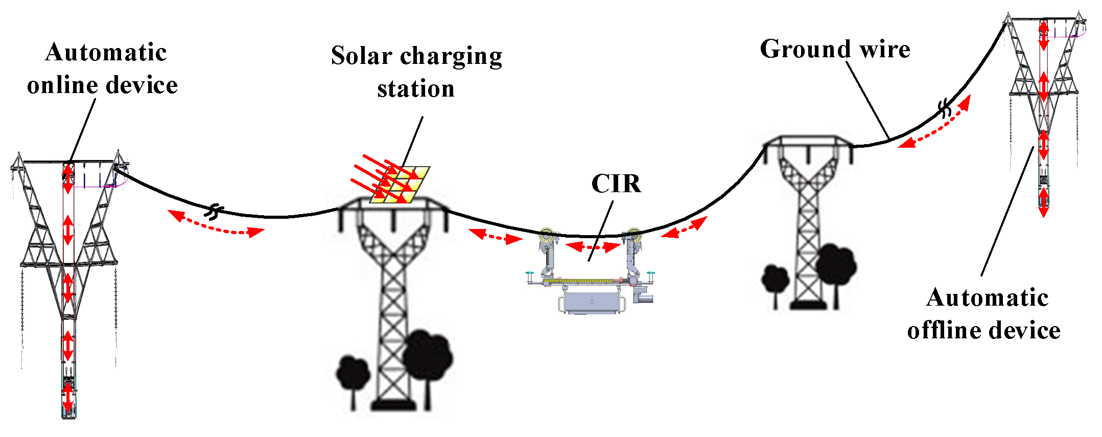
Figure 3.
The working principle of CIR LiDAR.
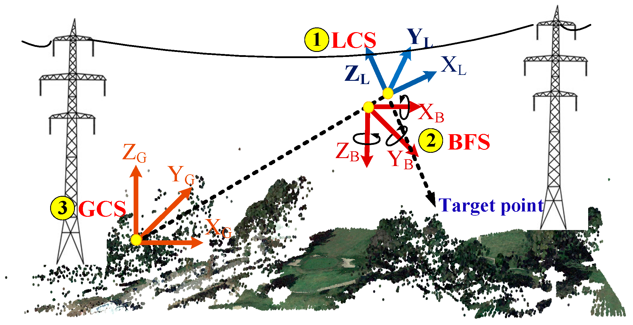
Figure 4.
Key components of CIR LiDAR system.

Figure 5.
Flow diagram of the power line extraction and reconstruction using CIR LiDAR data.
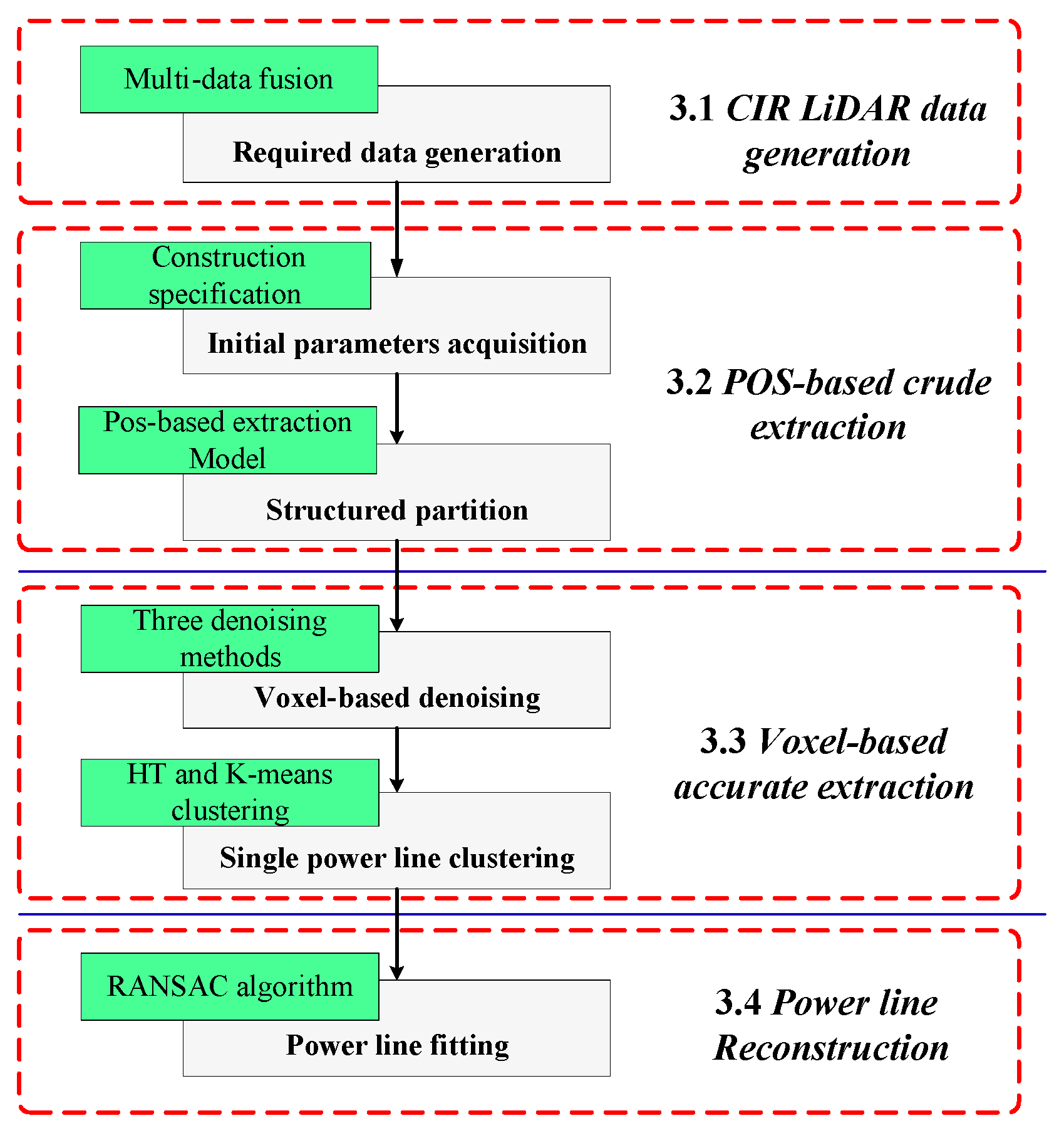
Figure 6.
Schematic diagram of quasi-scene of CIR LiDAR.

Figure 7.
The flow chart of data processing of CIR LiDAR.
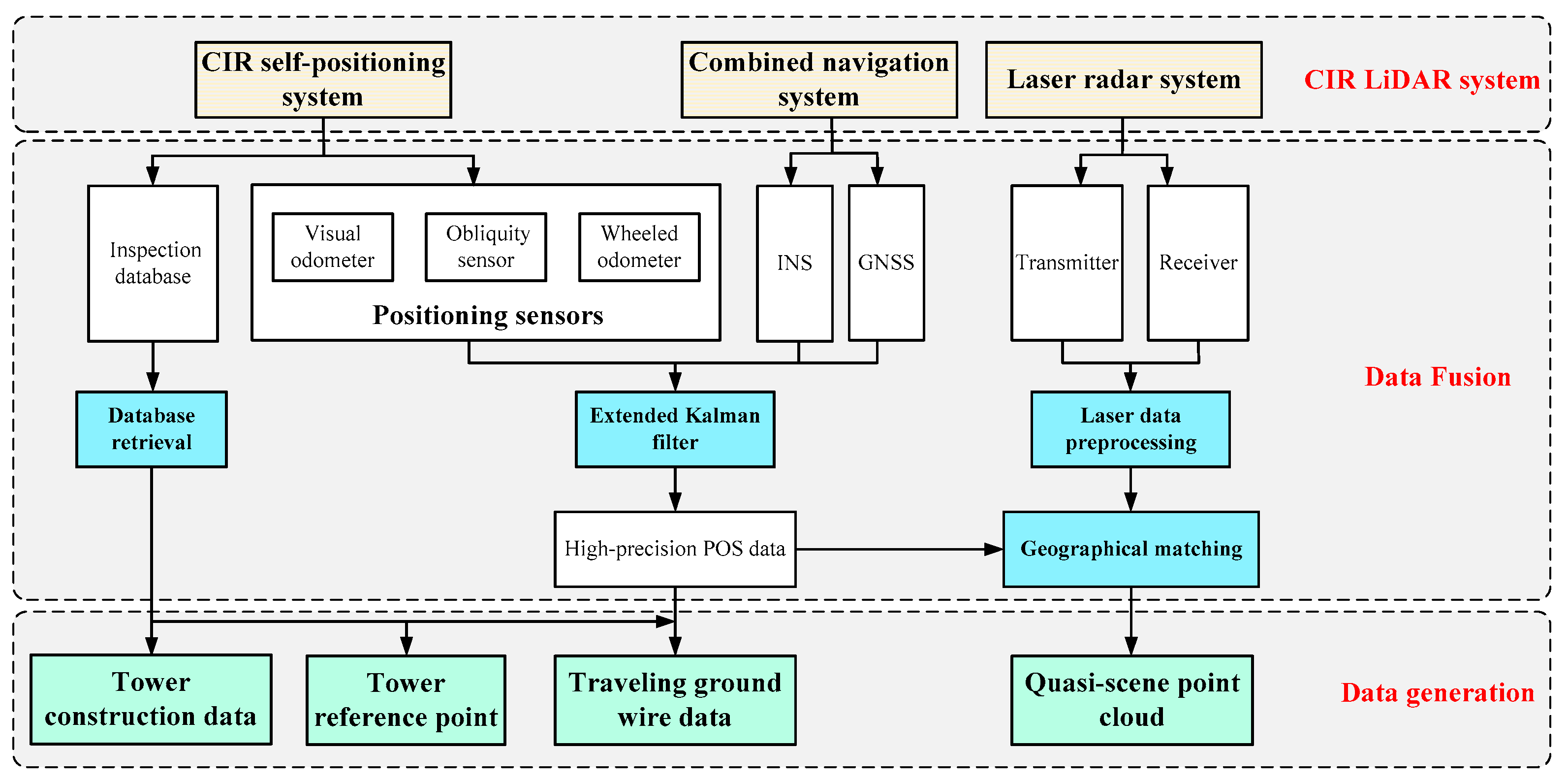
Figure 8.
Schematic diagram of double-loop two-bundle power lines.

Figure 9.
The construction process of OCP and ECS.

Figure 10.
The POS-based extraction model.

Figure 11.
Additional sag of the ground wire.
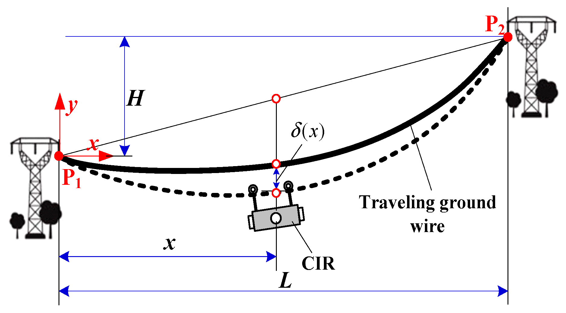
Figure 12.
Flow chart of voxel-based denoising.
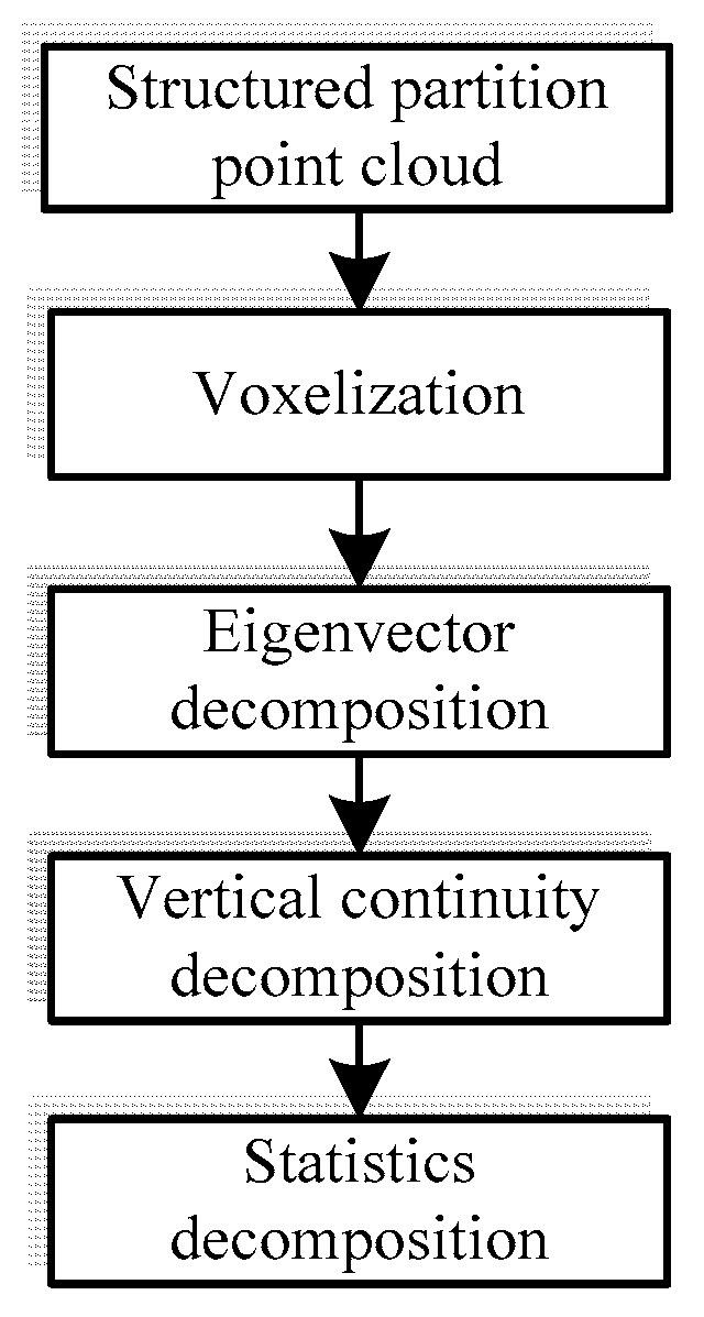
Figure 13.
Flow chart of single power line clustering.

Figure 14.
Photo of the test site.

Figure 15.
Point cloud of quasi-scene.

Figure 16.
POS-based crude extraction of test site.
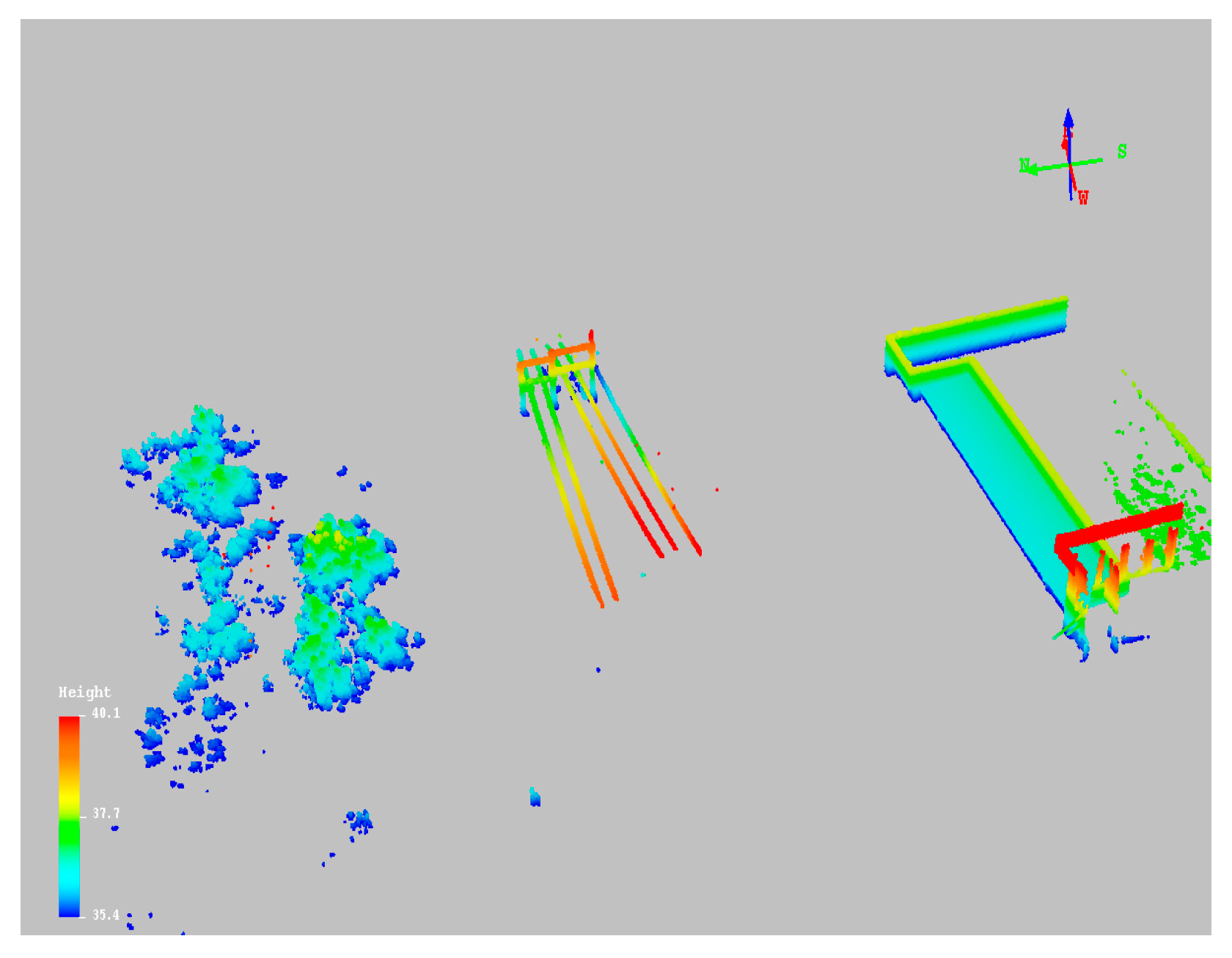
Figure 17.
Testing site data projected to the OCP: (a) point cloud of traveling ground wire; and (b) all power line point clouds.
Figure 17.
Testing site data projected to the OCP: (a) point cloud of traveling ground wire; and (b) all power line point clouds.

Figure 18.
Clustering result of Lines 1 and 2.
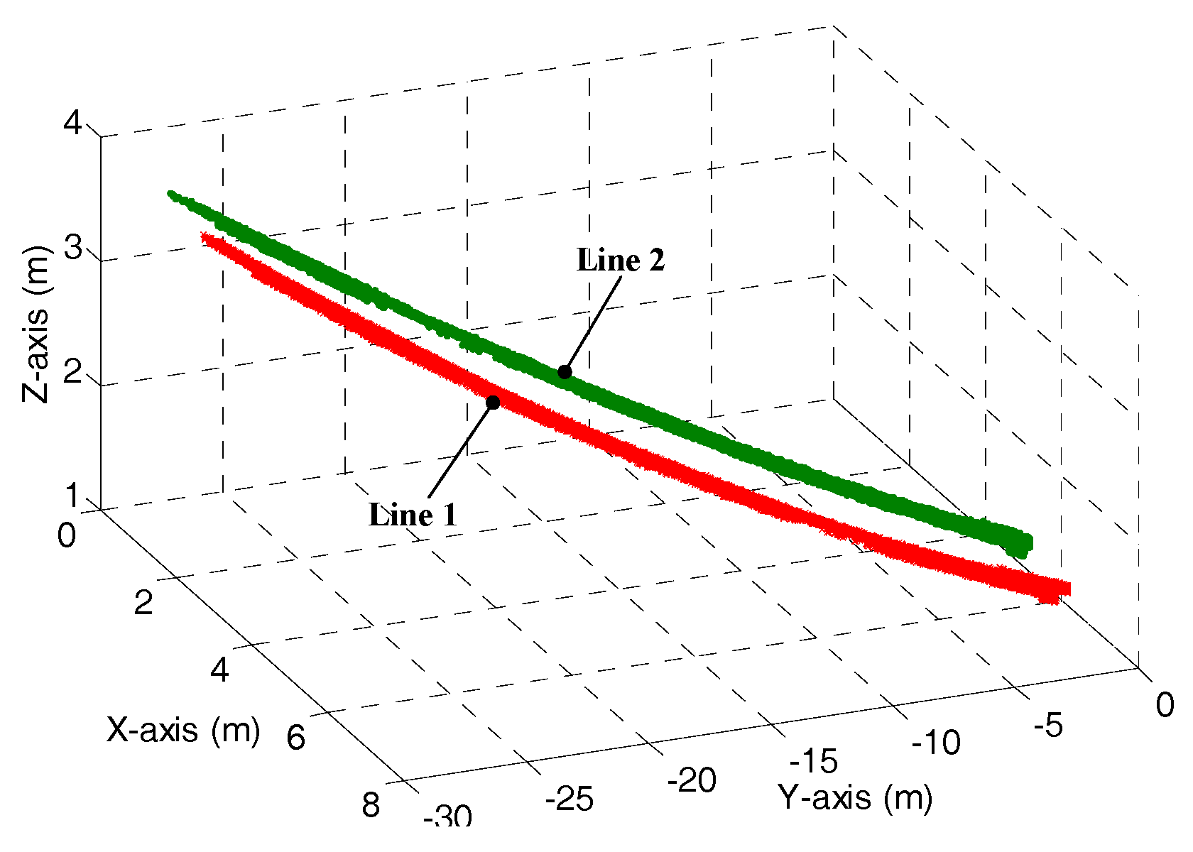
Figure 19.
Fitting models of all power lines.
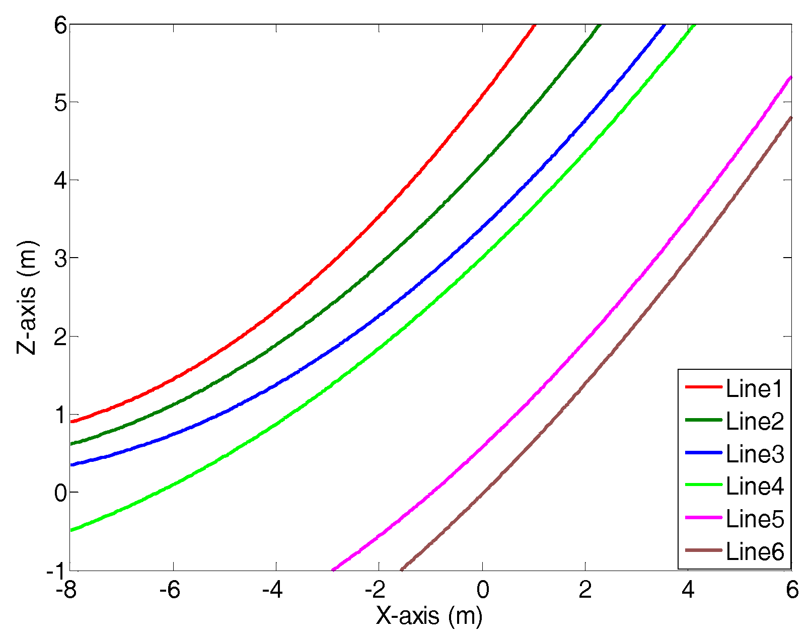
Figure 20.
Photo of the tower and power lines.
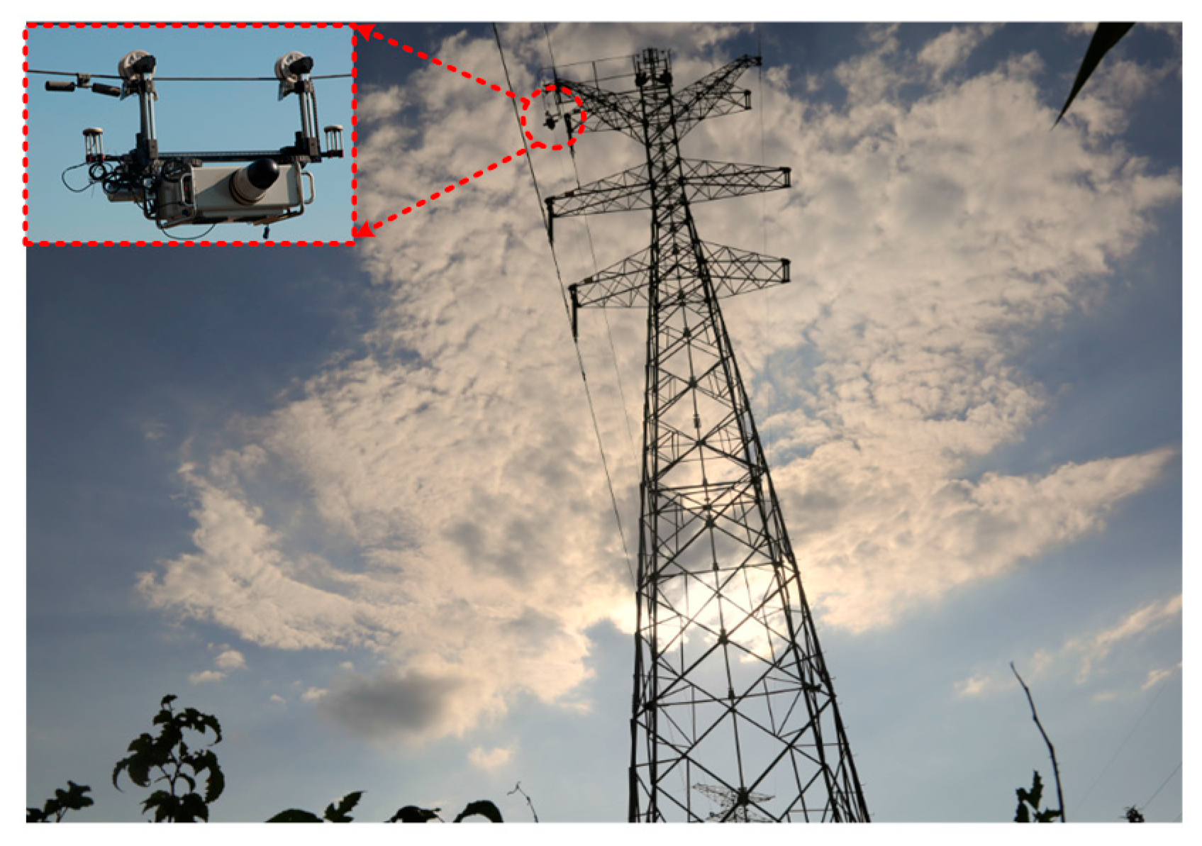
Figure 21.
The construction data of the tower.

Figure 22.
The quasi-scene point cloud of the actual lines.

Figure 23.
The POS-based crude extraction of the actual power lines.

Figure 24.
The experimental data cloud projected to OCP.

Figure 25.
The fitting model of the five power lines.

Table 1.
Evaluation of the results expressed as percentages.
| Line No. | Correct Points | Error Points | Omission Points | Correctness (%) | Integrality (%) | RMSE |
|---|---|---|---|---|---|---|
| 1 | 42881 | 0 | 0 | 100 | 100 | 0.0315 |
| 2 | 27583 | 1444 | 2716 | 95.0 | 91.0 | 0.0770 |
| 3 | 142041 | 4668 | 19873 | 96.8 | 87.7 | 0.0496 |
| 4 | 118350 | 5163 | 19236 | 95.8 | 86.0 | 0.0637 |
| 5 | 123753 | 6087 | 20569 | 95.3 | 85.7 | 0.0572 |
© 2017 by the authors. Licensee MDPI, Basel, Switzerland. This article is an open access article distributed under the terms and conditions of the Creative Commons Attribution (CC BY) license (http://creativecommons.org/licenses/by/4.0/).
Share and Cite
MDPI and ACS Style
Qin, X.; Wu, G.; Ye, X.; Huang, L.; Lei, J. A Novel Method to Reconstruct Overhead High-Voltage Power Lines Using Cable Inspection Robot LiDAR Data. Remote Sens. 2017, 9, 753. https://doi.org/10.3390/rs9070753
AMA Style
Qin X, Wu G, Ye X, Huang L, Lei J. A Novel Method to Reconstruct Overhead High-Voltage Power Lines Using Cable Inspection Robot LiDAR Data. Remote Sensing. 2017; 9(7):753. https://doi.org/10.3390/rs9070753
Chicago/Turabian StyleQin, Xinyan, Gongping Wu, Xuhui Ye, Le Huang, and Jin Lei. 2017. "A Novel Method to Reconstruct Overhead High-Voltage Power Lines Using Cable Inspection Robot LiDAR Data" Remote Sensing 9, no. 7: 753. https://doi.org/10.3390/rs9070753
Note that from the first issue of 2016, this journal uses article numbers instead of page numbers. See further details here.